ma 108 - ordinary differential equations - iit bombaydey/diffeqn_autumn13/lecture8.pdfma 108 -...
TRANSCRIPT

MA 108 - Ordinary Differential Equations
Santanu Dey
Department of Mathematics,Indian Institute of Technology Bombay,
Powai, Mumbai [email protected]
October 10, 2013
Santanu Dey Lecture 7

Outline of the lecture
Cauchy-Euler equations
Non-homogeneous equations
Santanu Dey Lecture 7

Cauchy-Euler Equations
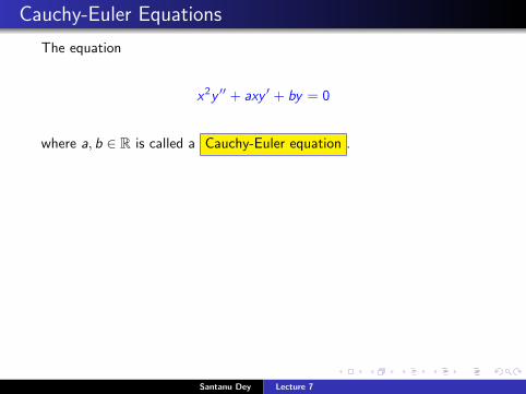
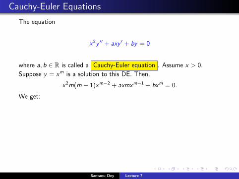
The equation
x2y ′′ + axy ′ + by = 0
where a, b ∈ R is called a Cauchy-Euler equation . Assume x > 0.
Suppose y = xm is a solution to this DE. Then,
x2m(m − 1)xm−2 + axmxm−1 + bxm = 0.
We get:
m(m − 1) + am + b = 0.
that is,m2 + (a− 1)m + b = 0.
This is called the auxiliary equation of the given Cauchy-Euler equation.The roots are
m1,m2 =(1− a)±
√(a− 1)2 − 4b
2.
Santanu Dey Lecture 7
Cauchy-Euler Equations
The equation
x2y ′′ + axy ′ + by = 0
where a, b ∈ R is called a Cauchy-Euler equation .
Assume x > 0.
Suppose y = xm is a solution to this DE. Then,
x2m(m − 1)xm−2 + axmxm−1 + bxm = 0.
We get:
m(m − 1) + am + b = 0.
that is,m2 + (a− 1)m + b = 0.
This is called the auxiliary equation of the given Cauchy-Euler equation.The roots are
m1,m2 =(1− a)±
√(a− 1)2 − 4b
2.
Santanu Dey Lecture 7

Cauchy-Euler Equations
The equation
x2y ′′ + axy ′ + by = 0
where a, b ∈ R is called a Cauchy-Euler equation . Assume x > 0.
Suppose y = xm is a solution to this DE. Then,
x2m(m − 1)xm−2 + axmxm−1 + bxm = 0.
We get:
m(m − 1) + am + b = 0.
that is,m2 + (a− 1)m + b = 0.
This is called the auxiliary equation of the given Cauchy-Euler equation.The roots are
m1,m2 =(1− a)±
√(a− 1)2 − 4b
2.
Santanu Dey Lecture 7

Cauchy-Euler Equations
The equation
x2y ′′ + axy ′ + by = 0
where a, b ∈ R is called a Cauchy-Euler equation . Assume x > 0.
Suppose y = xm is a solution to this DE.
Then,
x2m(m − 1)xm−2 + axmxm−1 + bxm = 0.
We get:
m(m − 1) + am + b = 0.
that is,m2 + (a− 1)m + b = 0.
This is called the auxiliary equation of the given Cauchy-Euler equation.The roots are
m1,m2 =(1− a)±
√(a− 1)2 − 4b
2.
Santanu Dey Lecture 7

Cauchy-Euler Equations
The equation
x2y ′′ + axy ′ + by = 0
where a, b ∈ R is called a Cauchy-Euler equation . Assume x > 0.
Suppose y = xm is a solution to this DE. Then,
x2m(m − 1)xm−2 + axmxm−1 + bxm = 0.
We get:
m(m − 1) + am + b = 0.
that is,m2 + (a− 1)m + b = 0.
This is called the auxiliary equation of the given Cauchy-Euler equation.The roots are
m1,m2 =(1− a)±
√(a− 1)2 − 4b
2.
Santanu Dey Lecture 7

Cauchy-Euler Equations
The equation
x2y ′′ + axy ′ + by = 0
where a, b ∈ R is called a Cauchy-Euler equation . Assume x > 0.
Suppose y = xm is a solution to this DE. Then,
x2m(m − 1)xm−2 + axmxm−1 + bxm = 0.
We get:
m(m − 1) + am + b = 0.
that is,m2 + (a− 1)m + b = 0.
This is called the auxiliary equation of the given Cauchy-Euler equation.
The roots are
m1,m2 =(1− a)±
√(a− 1)2 − 4b
2.
Santanu Dey Lecture 7

Cauchy-Euler Equations
The equation
x2y ′′ + axy ′ + by = 0
where a, b ∈ R is called a Cauchy-Euler equation . Assume x > 0.
Suppose y = xm is a solution to this DE. Then,
x2m(m − 1)xm−2 + axmxm−1 + bxm = 0.
We get:
m(m − 1) + am + b = 0.
that is,m2 + (a− 1)m + b = 0.
This is called the auxiliary equation of the given Cauchy-Euler equation.The roots are
m1,m2 =(1− a)±
√(a− 1)2 − 4b
2.
Santanu Dey Lecture 7

Cauchy-Euler Equations
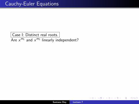
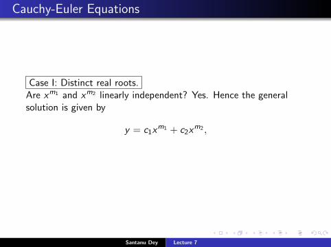
Case I: Distinct real roots.
Are xm1 and xm2 linearly independent? Yes. Hence the generalsolution is given by
y = c1xm1 + c2x
m2 ,
for c1, c2 ∈ R.
Santanu Dey Lecture 7
Cauchy-Euler Equations
Case I: Distinct real roots.Are xm1 and xm2 linearly independent?
Yes. Hence the generalsolution is given by
y = c1xm1 + c2x
m2 ,
for c1, c2 ∈ R.
Santanu Dey Lecture 7

Cauchy-Euler Equations
Case I: Distinct real roots.Are xm1 and xm2 linearly independent? Yes.
Hence the generalsolution is given by
y = c1xm1 + c2x
m2 ,
for c1, c2 ∈ R.
Santanu Dey Lecture 7

Cauchy-Euler Equations
Case I: Distinct real roots.Are xm1 and xm2 linearly independent? Yes. Hence the generalsolution is given by
y = c1xm1 + c2x
m2 ,
for c1, c2 ∈ R.
Santanu Dey Lecture 7
Cauchy-Euler Equations
Case I: Distinct real roots.Are xm1 and xm2 linearly independent? Yes. Hence the generalsolution is given by
y = c1xm1 + c2x
m2 ,
for c1, c2 ∈ R.
Santanu Dey Lecture 7

Cauchy-Euler Equations
Case I: Distinct real roots.Are xm1 and xm2 linearly independent? Yes. Hence the generalsolution is given by
y = c1xm1 + c2x
m2 ,
for c1, c2 ∈ R.
Santanu Dey Lecture 7

Cauchy-Euler Equations
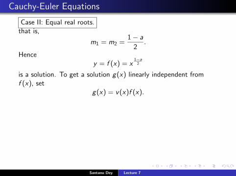
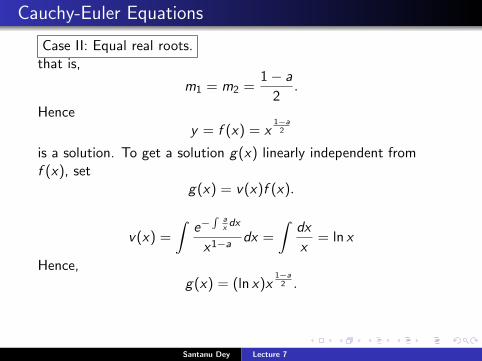
Case II: Equal real roots.
that is,
m1 = m2 =1− a
2.
Hencey = f (x) = x
1−a2
is a solution. To get a solution g(x) linearly independent fromf (x), set
g(x) = v(x)f (x).
v(x) =
∫e−
∫axdx
x1−adx =
∫dx
x= ln x
Hence,g(x) = (ln x)x
1−a2 .
Thus the general solution is given by
y = c1x1−a2 + c2x
1−a2 ln x ,
c1, c2 ∈ R.
Santanu Dey Lecture 7

Cauchy-Euler Equations
Case II: Equal real roots.that is,
m1 = m2 =1− a
2.
Hencey = f (x) = x
1−a2
is a solution.
To get a solution g(x) linearly independent fromf (x), set
g(x) = v(x)f (x).
v(x) =
∫e−
∫axdx
x1−adx =
∫dx
x= ln x
Hence,g(x) = (ln x)x
1−a2 .
Thus the general solution is given by
y = c1x1−a2 + c2x
1−a2 ln x ,
c1, c2 ∈ R.
Santanu Dey Lecture 7

Cauchy-Euler Equations
Case II: Equal real roots.that is,
m1 = m2 =1− a
2.
Hencey = f (x) = x
1−a2
is a solution. To get a solution g(x) linearly independent fromf (x),
setg(x) = v(x)f (x).
v(x) =
∫e−
∫axdx
x1−adx =
∫dx
x= ln x
Hence,g(x) = (ln x)x
1−a2 .
Thus the general solution is given by
y = c1x1−a2 + c2x
1−a2 ln x ,
c1, c2 ∈ R.
Santanu Dey Lecture 7
Cauchy-Euler Equations
Case II: Equal real roots.that is,
m1 = m2 =1− a
2.
Hencey = f (x) = x
1−a2
is a solution. To get a solution g(x) linearly independent fromf (x), set
g(x) = v(x)f (x).
v(x) =
∫e−
∫axdx
x1−adx =
∫dx
x= ln x
Hence,g(x) = (ln x)x
1−a2 .
Thus the general solution is given by
y = c1x1−a2 + c2x
1−a2 ln x ,
c1, c2 ∈ R.
Santanu Dey Lecture 7

Cauchy-Euler Equations
Case II: Equal real roots.that is,
m1 = m2 =1− a
2.
Hencey = f (x) = x
1−a2
is a solution. To get a solution g(x) linearly independent fromf (x), set
g(x) = v(x)f (x).
v(x) =
∫e−
∫axdx
x1−adx =
∫dx
x= ln x
Hence,g(x) = (ln x)x
1−a2 .
Thus the general solution is given by
y = c1x1−a2 + c2x
1−a2 ln x ,
c1, c2 ∈ R. Santanu Dey Lecture 7

Cauchy-Euler Equations
Case III : Complex roots
Roots are m1 = µ+ ıν, m2 = µ− ıν.
xm1 = xµeıν ln x = xµ(cos(ν ln x) + ı sin(ν ln x)),
xm2 = xµe−ıν ln x = xµ(cos(ν ln x)− ı sin(ν ln x)),
General solution is given by
y = xµ(c1 cos(ν ln x) + c2 sin(ν ln x)),
c1, c2 ∈ R.
Santanu Dey Lecture 7

Cauchy-Euler Equations
Case III : Complex roots
Roots are m1 = µ+ ıν, m2 = µ− ıν.
xm1 = xµeıν ln x = xµ(cos(ν ln x) + ı sin(ν ln x)),
xm2 = xµe−ıν ln x = xµ(cos(ν ln x)− ı sin(ν ln x)),
General solution is given by
y = xµ(c1 cos(ν ln x) + c2 sin(ν ln x)),
c1, c2 ∈ R.
Santanu Dey Lecture 7

Cauchy-Euler Equations
Case III : Complex roots
Roots are m1 = µ+ ıν, m2 = µ− ıν.
xm1 = xµeıν ln x = xµ(cos(ν ln x) + ı sin(ν ln x)),
xm2 = xµe−ıν ln x = xµ(cos(ν ln x)− ı sin(ν ln x)),
General solution is given by
y = xµ(c1 cos(ν ln x) + c2 sin(ν ln x)),
c1, c2 ∈ R.
Santanu Dey Lecture 7

Cauchy-Euler Equations
Case III : Complex roots
Roots are m1 = µ+ ıν, m2 = µ− ıν.
xm1 = xµeıν ln x = xµ(cos(ν ln x) + ı sin(ν ln x)),
xm2 = xµe−ıν ln x = xµ(cos(ν ln x)− ı sin(ν ln x)),
General solution is given by
y = xµ(c1 cos(ν ln x) + c2 sin(ν ln x)),
c1, c2 ∈ R.
Santanu Dey Lecture 7

Cauchy-Euler Equations
Case III : Complex roots
Roots are m1 = µ+ ıν, m2 = µ− ıν.
xm1 = xµeıν ln x = xµ(cos(ν ln x) + ı sin(ν ln x)),
xm2 = xµe−ıν ln x = xµ(cos(ν ln x)− ı sin(ν ln x)),
General solution is given by
y = xµ(c1 cos(ν ln x) + c2 sin(ν ln x)),
c1, c2 ∈ R.
Santanu Dey Lecture 7

Examples
Solve:
1 2x2y ′′ + 3xy ′ − y = 0, x > 0.
2 x2y ′′ + 5xy ′ + 4y = 0, x > 0.
3 x2y ′′ + xy ′ + y = 0, x > 0.
Solutions :
1 y = c1√x + c2/x
2 y = x−2(c1 + c2 ln x).
3 y = c1 cos(ln x) + c2 sin(ln x).
Santanu Dey Lecture 7

Examples
Solve:
1 2x2y ′′ + 3xy ′ − y = 0, x > 0.
2 x2y ′′ + 5xy ′ + 4y = 0, x > 0.
3 x2y ′′ + xy ′ + y = 0, x > 0.
Solutions :
1 y = c1√x + c2/x
2 y = x−2(c1 + c2 ln x).
3 y = c1 cos(ln x) + c2 sin(ln x).
Santanu Dey Lecture 7

Examples
Solve:
1 2x2y ′′ + 3xy ′ − y = 0, x > 0.
2 x2y ′′ + 5xy ′ + 4y = 0, x > 0.
3 x2y ′′ + xy ′ + y = 0, x > 0.
Solutions :
1 y = c1√x + c2/x
2 y = x−2(c1 + c2 ln x).
3 y = c1 cos(ln x) + c2 sin(ln x).
Santanu Dey Lecture 7

Examples
Solve:
1 2x2y ′′ + 3xy ′ − y = 0, x > 0.
2 x2y ′′ + 5xy ′ + 4y = 0, x > 0.
3 x2y ′′ + xy ′ + y = 0, x > 0.
Solutions :
1 y = c1√x + c2/x
2 y = x−2(c1 + c2 ln x).
3 y = c1 cos(ln x) + c2 sin(ln x).
Santanu Dey Lecture 7

Examples
Solve:
1 2x2y ′′ + 3xy ′ − y = 0, x > 0.
2 x2y ′′ + 5xy ′ + 4y = 0, x > 0.
3 x2y ′′ + xy ′ + y = 0, x > 0.
Solutions :
1 y = c1√x + c2/x
2 y = x−2(c1 + c2 ln x).
3 y = c1 cos(ln x) + c2 sin(ln x).
Santanu Dey Lecture 7

Examples
Solve:
1 2x2y ′′ + 3xy ′ − y = 0, x > 0.
2 x2y ′′ + 5xy ′ + 4y = 0, x > 0.
3 x2y ′′ + xy ′ + y = 0, x > 0.
Solutions :
1 y = c1√x + c2/x
2 y = x−2(c1 + c2 ln x).
3 y = c1 cos(ln x) + c2 sin(ln x).
Santanu Dey Lecture 7

Non-homogeneous Second Order Linear ODE’s
Consider the non-homogeneous DE
y ′′ + p(x)y ′ + q(x)y = r(x)
where p(x), q(x), r(x) are continuous functions on an interval I .
The associated homogeneous DE is
y ′′ + p(x)y ′ + q(x)y = 0.
Can we relate the solutions of the above two DE’s?
Santanu Dey Lecture 7

Non-homogeneous Second Order Linear ODE’s
Consider the non-homogeneous DE
y ′′ + p(x)y ′ + q(x)y = r(x)
where p(x), q(x), r(x) are continuous functions on an interval I .The associated homogeneous DE is
y ′′ + p(x)y ′ + q(x)y = 0.
Can we relate the solutions of the above two DE’s?
Santanu Dey Lecture 7

Non-homogeneous Second Order Linear ODE’s
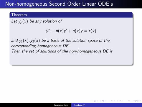
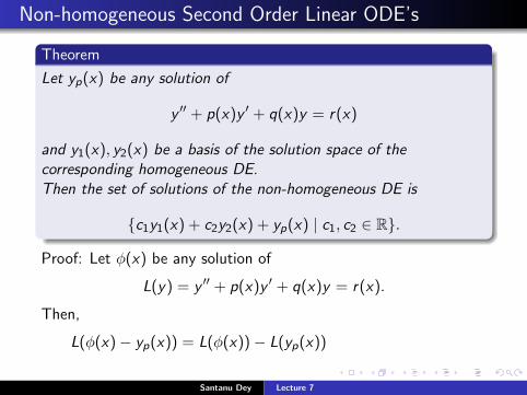
Theorem
Let yp(x) be any solution of
y ′′ + p(x)y ′ + q(x)y = r(x)
and y1(x), y2(x) be a basis of the solution space of thecorresponding homogeneous DE.Then the set of solutions of the non-homogeneous DE is
{c1y1(x) + c2y2(x) + yp(x) | c1, c2 ∈ R}.
Proof: Let φ(x) be any solution of
L(y) = y ′′ + p(x)y ′ + q(x)y = r(x).
Then,
L(φ(x)− yp(x)) = L(φ(x))− L(yp(x)) = r(x)− r(x) = 0.
Santanu Dey Lecture 7

Non-homogeneous Second Order Linear ODE’s
Theorem
Let yp(x) be any solution of
y ′′ + p(x)y ′ + q(x)y = r(x)
and y1(x), y2(x) be a basis of the solution space of thecorresponding homogeneous DE.
Then the set of solutions of the non-homogeneous DE is
{c1y1(x) + c2y2(x) + yp(x) | c1, c2 ∈ R}.
Proof: Let φ(x) be any solution of
L(y) = y ′′ + p(x)y ′ + q(x)y = r(x).
Then,
L(φ(x)− yp(x)) = L(φ(x))− L(yp(x)) = r(x)− r(x) = 0.
Santanu Dey Lecture 7
Non-homogeneous Second Order Linear ODE’s
Theorem
Let yp(x) be any solution of
y ′′ + p(x)y ′ + q(x)y = r(x)
and y1(x), y2(x) be a basis of the solution space of thecorresponding homogeneous DE.Then the set of solutions of the non-homogeneous DE is
{c1y1(x) + c2y2(x) + yp(x) | c1, c2 ∈ R}.
Proof: Let φ(x) be any solution of
L(y) = y ′′ + p(x)y ′ + q(x)y = r(x).
Then,
L(φ(x)− yp(x)) = L(φ(x))− L(yp(x)) = r(x)− r(x) = 0.
Santanu Dey Lecture 7

Non-homogeneous Second Order Linear ODE’s
Theorem
Let yp(x) be any solution of
y ′′ + p(x)y ′ + q(x)y = r(x)
and y1(x), y2(x) be a basis of the solution space of thecorresponding homogeneous DE.Then the set of solutions of the non-homogeneous DE is
{c1y1(x) + c2y2(x) + yp(x) | c1, c2 ∈ R}.
Proof:
Let φ(x) be any solution of
L(y) = y ′′ + p(x)y ′ + q(x)y = r(x).
Then,
L(φ(x)− yp(x)) = L(φ(x))− L(yp(x)) = r(x)− r(x) = 0.
Santanu Dey Lecture 7

Non-homogeneous Second Order Linear ODE’s
Theorem
Let yp(x) be any solution of
y ′′ + p(x)y ′ + q(x)y = r(x)
and y1(x), y2(x) be a basis of the solution space of thecorresponding homogeneous DE.Then the set of solutions of the non-homogeneous DE is
{c1y1(x) + c2y2(x) + yp(x) | c1, c2 ∈ R}.
Proof: Let φ(x) be any solution of
L(y) = y ′′ + p(x)y ′ + q(x)y = r(x).
Then,
L(φ(x)− yp(x)) = L(φ(x))− L(yp(x)) = r(x)− r(x) = 0.
Santanu Dey Lecture 7

Non-homogeneous Second Order Linear ODE’s
Theorem
Let yp(x) be any solution of
y ′′ + p(x)y ′ + q(x)y = r(x)
and y1(x), y2(x) be a basis of the solution space of thecorresponding homogeneous DE.Then the set of solutions of the non-homogeneous DE is
{c1y1(x) + c2y2(x) + yp(x) | c1, c2 ∈ R}.
Proof: Let φ(x) be any solution of
L(y) = y ′′ + p(x)y ′ + q(x)y = r(x).
Then,
L(φ(x)− yp(x))
= L(φ(x))− L(yp(x)) = r(x)− r(x) = 0.
Santanu Dey Lecture 7
Non-homogeneous Second Order Linear ODE’s
Theorem
Let yp(x) be any solution of
y ′′ + p(x)y ′ + q(x)y = r(x)
and y1(x), y2(x) be a basis of the solution space of thecorresponding homogeneous DE.Then the set of solutions of the non-homogeneous DE is
{c1y1(x) + c2y2(x) + yp(x) | c1, c2 ∈ R}.
Proof: Let φ(x) be any solution of
L(y) = y ′′ + p(x)y ′ + q(x)y = r(x).
Then,
L(φ(x)− yp(x)) = L(φ(x))− L(yp(x))
= r(x)− r(x) = 0.
Santanu Dey Lecture 7

Non-homogeneous Second Order Linear ODE’s
Theorem
Let yp(x) be any solution of
y ′′ + p(x)y ′ + q(x)y = r(x)
and y1(x), y2(x) be a basis of the solution space of thecorresponding homogeneous DE.Then the set of solutions of the non-homogeneous DE is
{c1y1(x) + c2y2(x) + yp(x) | c1, c2 ∈ R}.
Proof: Let φ(x) be any solution of
L(y) = y ′′ + p(x)y ′ + q(x)y = r(x).
Then,
L(φ(x)− yp(x)) = L(φ(x))− L(yp(x)) = r(x)− r(x) = 0.
Santanu Dey Lecture 7

Non-homogeneous Second Order Linear ODE’s
Hence, φ(x)− yp(x) is a solution of the homogeneous DE.
Thus,
φ(x)− yp(x) = c1y1(x) + c2y2(x),
for c1, c2 ∈ R. Hence,
φ(x) = c1y1(x) + c2y2(x) + yp(x).
Summary: In order to find the general solution of anon-homogeneous DE, we need to
get one particular solution of the non-homogeneous DE
get the general solution of the corresponding homogeneousDE.
Santanu Dey Lecture 7

Non-homogeneous Second Order Linear ODE’s
Hence, φ(x)− yp(x) is a solution of the homogeneous DE. Thus,
φ(x)− yp(x) = c1y1(x) + c2y2(x),
for c1, c2 ∈ R.
Hence,
φ(x) = c1y1(x) + c2y2(x) + yp(x).
Summary: In order to find the general solution of anon-homogeneous DE, we need to
get one particular solution of the non-homogeneous DE
get the general solution of the corresponding homogeneousDE.
Santanu Dey Lecture 7

Non-homogeneous Second Order Linear ODE’s
Hence, φ(x)− yp(x) is a solution of the homogeneous DE. Thus,
φ(x)− yp(x) = c1y1(x) + c2y2(x),
for c1, c2 ∈ R. Hence,
φ(x) = c1y1(x) + c2y2(x) + yp(x).
Summary: In order to find the general solution of anon-homogeneous DE, we need to
get one particular solution of the non-homogeneous DE
get the general solution of the corresponding homogeneousDE.
Santanu Dey Lecture 7

Non-homogeneous Second Order Linear ODE’s
Hence, φ(x)− yp(x) is a solution of the homogeneous DE. Thus,
φ(x)− yp(x) = c1y1(x) + c2y2(x),
for c1, c2 ∈ R. Hence,
φ(x) = c1y1(x) + c2y2(x) + yp(x).
Summary:
In order to find the general solution of anon-homogeneous DE, we need to
get one particular solution of the non-homogeneous DE
get the general solution of the corresponding homogeneousDE.
Santanu Dey Lecture 7

Non-homogeneous Second Order Linear ODE’s
Hence, φ(x)− yp(x) is a solution of the homogeneous DE. Thus,
φ(x)− yp(x) = c1y1(x) + c2y2(x),
for c1, c2 ∈ R. Hence,
φ(x) = c1y1(x) + c2y2(x) + yp(x).
Summary: In order to find the general solution of anon-homogeneous DE, we need to
get one particular solution of the non-homogeneous DE
get the general solution of the corresponding homogeneousDE.
Santanu Dey Lecture 7

Non-homogeneous Second Order Linear ODE’s
Hence, φ(x)− yp(x) is a solution of the homogeneous DE. Thus,
φ(x)− yp(x) = c1y1(x) + c2y2(x),
for c1, c2 ∈ R. Hence,
φ(x) = c1y1(x) + c2y2(x) + yp(x).
Summary: In order to find the general solution of anon-homogeneous DE, we need to
get one particular solution of the non-homogeneous DE
get the general solution of the corresponding homogeneousDE.
Santanu Dey Lecture 7