2nd ISSMO/AIAA Internet Conferen eon Approximations and Fast Reanalysis in Engineering OptimizationMay 25 { June 2, 2000Redu ed-Basis Output-BoundMethods for Ellipti PartialDi�erential Equations1Dimitrios V. RovasDepartment of Me hani al Engineering, Room 3-243,Massa husetts Institute of Te hnology, Cambridge, MA,02139-4307, rovas�mit.eduAnthony T. PateraDepartment of Me hani al Engineering, Room 3-264,Massa husetts Institute of Te hnology, Cambridge, MA,02139-4307, patera�mit.eduAbstra t2 We present a two-stage o�-line/on-line bla kbox redu ed-basis output bound methodfor the predi tion of outputs of interest asso iatedwith ellipti partial di�erential equations with aÆneparameter dependen e. The method is hara ter-ized by (i) Galerkin proje tion onto a redu ed-basisspa e omprising solutions at sele ted points in pa-rameter spa e, and (ii) a rigorous output error boundbased on the dual norm of the resulting residual.The omputational omplexity of the on-line stage ofthe pro edure s ales only with the dimension of theredu ed-basis spa e and the parametri omplexityof the partial di�erential operator. The method isthus both eÆ ient and ertain: thanks to the a pos-teriori error bounds, we may safely retain only theminimal number of modes ne essary to a hieve thepres ribed a ura y in the output of interest. Thete hnique is parti ularly appropriate for appli ationssu h as design, optimization, and ontrol, in whi hrepeated and rapid evaluation of the output is re-quired; in the limit of many evaluations, the method an be several orders of magnitude faster than stan-dard (�nite element) approximation. To illustratethe method, we onsider the design of a thermal �n.

1. MotivationTo motivate and illustrate our methods we onsidera spe i� example, a thermal �n. The �n, shownin Figure 1, onsists of a entral \post" and fourhorizontal plates whi h we denote \sub�ns;" the �n ondu ts heat from a pres ribed ux \sour e" at theroot through the large-surfa e-area sub�ns to sur-rounding owing air. The �n is hara terized byseven design parameters, or \inputs," � 2 D �IRP=7, where �i = ki; i = 1; : : : ; 4; �5 = Bi; �6 = L;and �7 = t. Here ki is the thermal ondu tivity ofthe ith sub�n (normalized relative to the post on-du tivity); Bi is the Biot number, a nondimensionalheat transfer oeÆ ient re e ting onve tive trans-port to the air at the �n surfa es; and L and t arethe length and thi kness of the sub�ns (normalizedrelative to the post width). The performan e metri ,or \output," s 2 IR, is hosen to be the average tem-perature of the �n root normalized by the pres ribedheat ux into the �n root, �root.Figure 1We an express our input-output relationship ass = `O(u(�)), where `O(v) is a ( ontinuous) lin-ear fun tional | `O(v) = R�root v | and u(�) isthe temperature distribution within the �n. (The1The material presented in this arti le is an expository version of work performed in ollaboration with Dr. Lu Ma hiels ofLawren e Livermore National Laboratory and Professor Yvon Maday of University of Paris VI and reported in greater detailin referen es [1, 2, 3, 4℄. We also thank Professor Jaime Peraire of MIT, Professor Einar R�nquist of Norwegian Universityof S ien e and Te hnology, Mr. Roland Von Kaenel of EPFL, and Ms. Shidrati Ali of National University of Singapore{Singapore-MIT Allian e for helpful omments. The work is supported by AFOSR, NASA Langley Resear h Center, and theSingapore-MIT Allian e.2This arti le will appear in the next issue of the SIAM SIAG/OPT Views-and-News (ed. N. Alexandrov).1

temperature �eld is of ourse a fun tion of the spa-tial oordinate, x; we expli itly indi ate this depen-den e only as needed.) The temperature distributionu(�) 2 Y satis�es the weak form of the ellipti par-tial di�erential equation des ribing heat ondu tionin the �n, a(u; v;�) = `(v);8v 2 Y ; (1)a(u; v;�) is the weak representation of the Lapla ian,and `(v) re e ts the pres ribed heat ux at the root.Here Y is the appropriate Hilbert spa e with asso i-ated inner produ t (�; �)Y and indu ed norm k �kY 3.The bilinear form a(�; �;�) is symmetri , a(w; v;�) =a(v; w;�);8w; v 2 Y 2;8� 2 D; uniformly ontinu-ous, ja(w; v;�)j � kwkY kvkY ;8w; v 2 Y 2;8� 2 D;and oer ive, �kvk2Y � a(v; v;�);8v 2 Y;8� 2 D.Here � and are positive real onstants. Finally,the form `(v) is a linear bounded fun tional; for our hoi e of s aling and output, `O(v) = `(v), whi h wewill exploit to simplify the exposition.It is readily shown that our form a an be ex-pressed asa(w; v;�) = QXq=1�q(�)aq(w; v);8w; v 2 Y 2;8� 2 D;(2)for appropriately hosen fun tions �q:D ! IR andasso iated �-independent bilinear forms aq:Y �Y !IR, q = 1; : : : ; Q: the parameter dependen e is thus\aÆne" or \separable." Note that we pose our prob-lem on a �xed �n referen e domain in order toensure that the parametri dependen e on geometry| L and t | enters through a(�; �;�) and ultimatelythe �q(�). For our parti ular problem, Q = 15; if wefreeze (�x) all parameters ex ept L and t (su h thatPe� = 2), Q = 8; if we freeze only L and t (su h thatPe� = 5), Q = 6.Our goal is to onstru t an approximation to u,~u, and hen e approximation to s, ~s = `O(~u), whi h is(i) erti�ably a urate, and (ii) very eÆ ient in thelimit of many evaluations. By the latter we meanthat, following an initial �xed investment, the addi-tional in remental ost to evaluate ~s(�) for any new� 2 D is mu h less than the e�ort required to dire tly ompute s(�) = `O(u(�)) by (say) standard �niteelement approximation. This de�nition of eÆ ien y

is parti ularly appropriate in the ontext of design,optimization, and ontrol, in whi h we require veryrapid response and many output evaluations.2. Redu ed-Basis ApproximationRedu ed-basis methods (e.g., [5, 6, 7℄) are a now- lassi al approa h that are a spe ial \parameter-spa e" version of weighted{residual (here Galerkin)approximation. To de�ne the (or a) redu ed{basispro edure, we �rst introdu e a sample in param-eter spa e, SN = f�1; : : : ; �Ng, and asso iatedredu ed-basis spa e WN = spanf�1 � u(�1); �2 �u(�2); : : : ; �N � u(�N )g; where u(�i) satis�es (1) for� = �i 2 D (note �i refers to the ith omponent ofthe P{tuple �, whereas �i refers to the ith P{tuplein SN ). We then require our redu ed-basis approxi-mation to u(�) for any given �, uN (�) 2 WN � Y ,to satisfy a(uN (�); v;�) = `(v);8v 2WN ; (3)the redu ed-basis approximation to s(�) an subse-quently be evaluated as sN (�) = `O(uN (�)).It is a simple matter to show thatku(�)�uN (�)kY � r � minwN2WN ku(�)�wNkY ; (4)whi h states that our approximation is in some senseoptimal in the Y norm. It an also be readily shownfor our parti ular problem thats(�) = sN (�) + a(eN (�); eN (�);�); (5)where eN = u� uN . It follows from (4),(5), and the ontinuity of a thatjs(�)� sN (�)j � 2� ( minwN2WN ku(�)� wNkY )2; (6)thus our output approximation is also optimal insome sense.We must, of ourse, also understand the extentto whi h the best wN in WN an, indeed, approx-imate the requisite temperature distribution. Theessential point is that, although WN learly doesnot have any approximation properties for general3Here Y = H1(), the spa e of fun tions that are square integrable and that have square integrable �rst (distributional)derivatives over the �n referen e domain . The inner produ t (w; v)Y may be hosen to be Rrw � rv + wv.2

fun tions in Y , simple interpolation arguments inparameter spa e suggest that WN should approxi-mate well u(�) even for very modest N ; indeed, ex-ponential onverge is obtained in N for suÆ ientlysmooth �-dependen e (e.g., [6, 7℄). It is for thisreason that, even in high-dimensional (large P ) pa-rameter spa es, redu ed-basis methods ontinue toperform well | mu h better than \non-state-spa e"dire t interpolation of (�; s(�)) input-output pairs.In some sense, redu ed-basis methods transform ex-tensive parameter-spa e exploration from a probleminto an opportunity.We now turn to the omputational issues. We�rst express the redu ed-basis approximation asuN (x;�) = NXj=1uNj (�)�j(x) = (uN (�))T �(x); (7)and hoose for test fun tions v = �i(x); i = 1; : : : ; N .We then insert these representations into (3) to yieldthe desired algebrai equations for uN (�) 2 IRN ,NXj=1 a(�j ; �i;�)uNj = `(�i); i = 1; : : : ; N: (8)Equation (8) an be written in matrix form asA(�)uN (�) = L; (9)where A(�) 2 IRN�N is the SPD matrix with entriesAi;j(�) = a(�j ; �i;�); 1 � i; j � N , and L 2 IRN isthe \load" ve tor with entries Li = `(�i); 1 � i � N .We now evoke (2) to note thatAi;j(�) = a(�j ; �i;�) = QXq=1�q(�)aq(�j ; �i)= QXq=1 �q(�)Aqi;j ; (10)where the matri es Aq 2 IRN�N are given by Aqi;j =aq(�j ; �i); 1 � i; j � N; q = 1; : : : ; Q. The o�-line/on-line de omposition is now lear. In the o�-line stage, we onstru t the Aq; q = 1; : : : ; Q. In theon-line stage, for any given �, we �rst form A fromthe Aq a ording to (10); we next invert (9) to �nduN (�); and we then ompute sN (�) = `O(uN (�)) =`(uN (�)) = (uN (�))TL. As we shall see, N will typ-i ally be O(10) for our parti ular problem. Thus,

as required, the in remental ost to evaluate sN (�)for any given new � is very small: O(N2Q) to formA(�); O(N3) to invert (the typi ally dense) A(�)system; and O(N) to evaluate sN (�) from uN (�).But all is not well. The above a priori results tellus only that we are doing as well as possible; it doesnot tell us how well we are doing. In parti ular, theerror in our output is not known, and hen e the min-imal number of basis fun tions required to satisfythe desired error toleran e an not be as ertained.As a result, either too many or too few fun tions areretained; the former results in omputational inef-� ien y, the latter in un ertainty and una eptablyina urate predi tions. We thus need a posteriorierror bounds as well.3. Output BoundsTo begin, we assume that we may �nd a fun tiong(�):D ! IR+ and symmetri ontinuous oer ivebilinear form a:Y � Y ! IR su h that kvk2Y � g(�)a(v; v) � a(v; v;�);8v 2 Y;8� 2 D;(11)for some real positive onstant ; for our thermal �nproblem we an readily �nd a g(�) and a(w; v) su hthat (11) is satis�ed. The pro edure is then simple:we �rst ompute e(�) 2 Y solution ofg(�)a(e(�); v) = R(v;�);8v 2 Y; (12)where R(v;�) � `(v)�a(uN ; v;�) is the residual; wethen evaluate our bounds assN� (�) = sN(�); sN+ (�) = sN (�) + �N (�); (13)where �N (�) = g(�)a(e(�); e(�)) (14)is the bound gap. The notion of output bounds isnot restri ted to redu ed{basis approximations: it an also be applied within the ontext of standard(adaptive) �nite element dis retization as well as it-erative (Krylov) solution strategies [8, 9℄.We an then show thatsN� (�) � s(�) � sN+ (�); 8N ; (15)we thus have a erti� ate of �delity for sN | it iswithin �N (�) of s(�). The proof of (15) is sim-ple. To prove the left inequality we need only ap-peal to (5) and the oer ivity of a. To demonstrate3

the right inequality we �rst note that R(eN (�);�) =`(eN (�))� a(uN (�); eN (�);�) = a(eN (�); eN (�);�),sin e `(eN (�)) = a(u; eN (�);�) from (1) for v =eN (�); we next hoose v = eN (�) in (12) to obtaing(�)a(e(�); eN (�)) = a(eN (�); eN (�);�); from thisresult and the right inequality of (11) we then have�N (�) � g(�)a(e; e)= g(�)a(e� eN ; e� eN ) + 2a(eN ; eN )� g(�)a(eN ; eN )� g(�)a(e� eN ; e� eN ) + a(eN ; eN );(16)from (16) and the left inequality of (11) we thus on- lude that �N (�) � a(eN ; eN ); a omparison of (5)and (13) then ompletes the proof.Our a posteriori bound result indi ates that,through �N , we an now as ertain the a ura yof our output predi tion, whi h will in turn per-mit us to adaptively modify our approximation untilany pres ribed error toleran e is satis�ed (see be-low). However, from the perspe tive of eÆ ien y, itis also riti al that �N (�) be a good error estima-tor; a poor estimator will en ourage us to unne -essarily re�ne an approximation whi h is, in fa t,adequate. To prevent the latter we would like thee�e tivity �N (�) � �N (�)=js(�) � sN (�)j to be or-der unity. For our problem it is simple to prove that�N (�) � = , and thus �N (�) is ertainly boundedindependent of � and N ; in pra ti e, e�e tivities aretypi ally less than 10, whi h is adequate given therapid onvergen e of redu ed-basis approximations.We now turn to the omputational issues. We�rst note that, from (2) and (7), (12) an be re-written asa(e(�); v) =1g(�) `(v)� QXq=1 NXj=1�q(�)uNj (�)aq(�j ; v)!;8v 2 Y: (17)We thus see from simple linear superposition thate(�) an be expressed ase(�) = 1g(�) (z0 + QXq=1 NXj=1�q(�)uNj (�)zqj ); (18)where z0 2 Y satis�es a(z0; v) = `(v);8v 2 Y;and zqj 2 Y; j = 1; : : : ; N; q = 1; : : : ; Q, satis�es

a(zqj ; v) = �aq(�j ; v);8v 2 Y: It then follows thatwe an express �N (�) of (14) as�N (�) = 1g(�)" a(z0; z0)| {z } 0 +2 QXq=1 NXj=1�q(�)uNj (�) a(z0; zqj )| {z }�qj +QXq=1 QXq0=1 NXj=1 NXj0=1�q(�)�q0(�)uNj (�)uNj0 (�) a(zqj ; zq0j0 )| {z }�qq0jj0 #;(19)sN+ (�) then dire tly follows from (13).The o�-line/on-line de omposition is now lear.In the o�-line stage we ompute z0 and zqj ; j =1; : : : ; N; q = 1; : : : ; Q, and then the inner produ ts 0;�qj , and �qq0jj0 de�ned in (19). In the on-line stage,for any given new �, and given sN (�) and uN (�)as omputed in the on-line stage of the output pre-di tion pro ess (Se tion 2), we �rst evaluate �N (�)as�N (�) = 1g(�)" 0 + 2 QXq=1 NXj=1�q(�)uNj (�)�qj +QXq=1 QXq0=1 NXj=1 NXj0=1�q(�)�q0(�)uNj (�)uNj0 (�)�qq0jj0#; (20)and then evaluate sN+ (�) = sN (�) +�N (�). The in- remental ost to evaluate sN+ (�) for any given new� is very small: O(N2Q2).4. Numeri al AlgorithmIn the simplest ase we take our �eld and output ap-proximations to be ~u(�) = uN (�) and ~s(�) = sN (�),respe tively, for some given N , and then ompute�N (�) to assess the error. However, it is veryeasy to improve upon this re ipe. To wit, we take~u(�) = u ~N (�) and ~s(�) = s ~N (�), where u ~N (�) ands ~N(�) are the redu ed-basis approximations asso i-ated with a subspa e ofWN ,W ~N , in whi h we sele tonly ~N of our available basis fun tions. In pra ti e,we in lude in W ~N the basis fun tions orresponding4

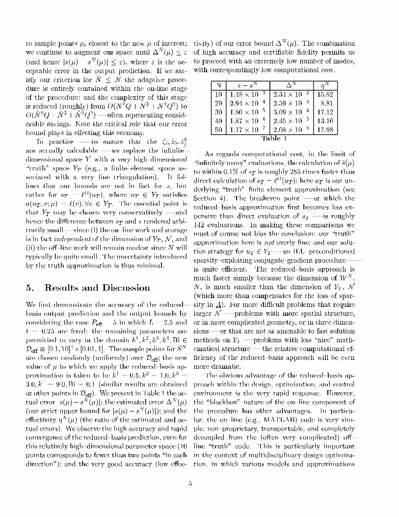
to sample points �i losest to the new � of interest;we ontinue to augment our spa e until � ~N (�) � "(and hen e js(�) � s ~N (�)j � "), where " is the a - eptable error in the output predi tion. If we sat-isfy our riterion for ~N � N the adaptive pro e-dure is entirely ontained within the on-line stageof the pro edure; and the omplexity of this stageis redu ed (roughly) from O(N2Q+N3 +N2Q2) toO( ~N2Q+ ~N3+ ~N2Q2) | often representing onsid-erable savings. Note the riti al role that our errorbound plays in e�e ting this e onomy.In pra ti e | to ensure that the �i; z0; zqjare a tually al ulable | we repla e the in�nite{dimensional spa e Y with a very high dimensional\truth" spa e YT (e.g., a �nite{element spa e as-so iated with a very �ne triangulation). It fol-lows that our bounds are not in fa t for s, butrather for sT = `O(uT ), where uT 2 YT satis�esa(uT ; v;�) = `(v);8v 2 YT . The essential point isthat YT may be hosen very onservatively | andhen e the di�eren e between sT and s rendered arbi-trarily small | sin e (i) the on{line work and storageis in fa t independent of the dimension of YT , N , and(ii) the o�{line work will remain modest sin e N willtypi ally be quite small. The un ertainty introdu edby the truth approximation is thus minimal.5. Results and Dis ussionWe �rst demonstrate the a ura y of the redu ed{basis output predi tion and the output bounds by onsidering the ase Pe� = 5 in whi h L = 2:5 andt = 0:25 are �xed; the remaining parameters arepermitted to vary in the domain k1; k2; k3; k4;Bi 2De� � [0:1; 10℄4�[0:01; 1℄. The sample points for SNare hosen randomly (uniformly) over De�; the newvalue of � to whi h we apply the redu ed{basis ap-proximation is taken to be k1 = 0:5; k2 = 1:0; k3 =3:0; k4 = 9:0;Bi = 0:1 (similar results are obtainedat other points inDe�). We present in Table 1 the a -tual error js(�)� sN (�)j; the estimated error �N (�)(our stri t upper bound for js(�)� sN (�)j); and thee�e tivity �N (�) (the ratio of the estimated and a -tual errors). We observe the high a ura y and rapid onvergen e of the redu ed{basis predi tion, even forthis relatively high{dimensional parameter spa e (10points orresponds to fewer than two points \in ea hdire tion"); and the very good a ura y (low e�e -

tivity) of our error bound �N (�). The ombinationof high a ura y and erti�able �delity permits usto pro eed with an extremely low number of modes,with orrespondingly low omputational ost.N js� sN j �N �N10 1:48 � 10�3 2:34 � 10�2 15.8220 2:94 � 10�4 2:59 � 10�3 8.8130 1:80 � 10�5 3:09 � 10�4 17.1240 1:87 � 10�6 2:45 � 10�5 13.1050 1:17 � 10�7 2:08 � 10�6 17.98Table 1As regards omputational ost, in the limit of\in�nitely many" evaluations, the al ulation of ~s(�)to within 0.1% of sT is roughly 285 times faster thandire t al ulation of sT = `O(uT ); here uT is our un-derlying \truth" �nite element approximation (seeSe tion 4). The breakeven point | at whi h theredu ed{basis approximation �rst be omes less ex-pensive than dire t evaluation of sT | is roughly142 evaluations. In making these omparisons wemust of ourse not bias the on lusion: our \truth"approximation here is not overly �ne; and our solu-tion strategy for uT 2 YT | an ILU{pre onditionedsparsity{exploiting onjugate{gradient pro edure |is quite eÆ ient. The redu ed{basis approa h ismu h faster simply be ause the dimension of WN ,N , is mu h smaller than the dimension of YT , N(whi h more than ompensates for the loss of spar-sity in A). For more diÆ ult problems that requirelarger N | problems with more spatial stru ture,or in more ompli ated geometry, or in three dimen-sions | or that are not as amenable to fast solutionmethods on YT | problems with less \ni e" math-emati al stru ture | the relative omputational ef-� ien y of the redu ed{basis approa h will be evenmore dramati .The obvious advantage of the redu ed{basis ap-proa h within the design, optimization, and ontrolenvironment is the very rapid response. However,the \bla kbox" nature of the on{line omponent ofthe pro edure has other advantages. In parti u-lar, the on{line (e.g., MATLAB) ode is very sim-ple, non{proprietary, transportable, and ompletelyde oupled from the (often very ompli ated) o�{line \truth" ode. This is parti ularly importantin the ontext of multidis iplinary design optimiza-tion, in whi h various models and approximations5

must be integrated. The bla kbox implementationalso suggests new approa hes to ele troni hand-books | parameter{spa e exploration through a -tionable equations that provide rapid and erti�ablya urate solutions to omplex problems.We lose this se tion with a more applied exam-ple. We now �x all parameters ex ept L and t, sothat Pe� = 2; (L; t) are permitted to vary withinDe� = [2:0; 3:0℄ � [0:1; 0:5℄. We hoose for our twooutputs the volume of the �n (easily al ulable of ourse), V, and the root average temperature (asde�ned above), s. As our \design exer ise" we now onstru t the a hievable set | all those (V; s) pairsasso iated with some (L; t) in D; the result, basedon many evaluations of (V; s ~N+ ) for di�erent valuesof (L; t) 2 De�, is shown in Figure 2. We present theresults in terms of s ~N+ rather than s ~N to ensure thatthe a tual temperature sT will always be lower thanour predi tions (that is, onservative within the on-text of the design problem); and we hoose ~N (seeSe tion 4) su h that s ~N+ is always within 0.1% of sTto ensure that the design pro ess is not misled byina urate predi tions. Note that, given the obviouspreferen es of lower volume and lower temperature,the designer will be most interested in the lower leftboundary of the a hievable set | the Pareto eÆ- ient frontier; although this boundary an of oursebe found without onstru ting the entire a hievableset, many evaluations of the outputs will still be re-quired.

19 20 21 22 23 24 25 26 274

6

8

10

12

14

16

Figure 2

6. Generalizations and IssuesMany (though not all) of the assumptions that wehave introdu ed are assumptions of onvenien e, notne essity, intended to simplify the exposition. First,the output fun tional `O need not be same as theinhomogeneity `; with the introdu tion of an adjoint(or dual) problem [2℄, all of our results above ex-tend to the more general ase. Se ond, the fun -tion g(�) need not be known a priori: g(�) is re-lated to an eigenvalue problem whi h an itself bereadily approximated by a redu ed{basis spa e on-stru ted as the span of appropriate eigenfun tions(in theory we an now only prove asymptoti bound-ing properties as N ! 1, however in pra ti e theredu ed{basis eigenvalue approximation onvergesvery rapidly, and there is thus little loss of ertainty).Third, these same notions extend, with some modi-� ation, to non oer ive problems, where g(�) is nowin fa t the inf{sup stability parameter [3, 4℄. Finally,nonsymmetri operators are readily treated, as are ertain lasses of nonlinearity in the state variables(e.g., eigenvalue problems [1℄ and Burgers equation).Perhaps the most limiting assumption is (2),aÆne dependen e on the parameter. In some ases(2) may indeed apply, but Q may be rather large. Insu h ases we an perhaps redu e the O(Q2) om-plexity and storage of the o�{line and on{line stagesto O(Q) by introdu ing a redu ed{basis approxima-tion of the error equation (12) for a suitably hosen\staggered" sample set SMerr and asso iated redu ed{basis spa e onstru ted as the span of appropriateerror fun tions. These ideas may also extend to the ase in whi h the parameter dependen e an not beexpressed (or a urately approximated) as in (2);however we would now need to at least partiallyabandon the bla kbox nature of the on{line stage of omputation, allowing evaluation (though not inver-sion) of the truth{approximation operator, as wellas storage of some redu ed{basis ve tors of size N .These methods are urrently under development; theideas of this �nal paragraph are at present spe ula-tive. REFERENCES[1℄ L. Ma hiels, Y. Maday, I.B. Oliveira, A.T. Pat-era, and D.V. Rovas. Output bounds for redu ed-basis approximations of symmetri positive de�nite6

eigenvalue problems. C. R. A ad. S i. Paris, S�erieI, to appear.[2℄ Y. Maday, L. Ma hiels, A.T. Patera, and D.V.Rovas. Bla kbox redu ed-basis output bound meth-ods for shape optimization. In Pro eedings 12thInternational Domain De omposition Conferen e,Chiba Japan, 2000, to appear.[3℄ D.V. Rovas. An overview of bla kbox redu ed-basisoutput bound methods for ellipti partial di�eren-tial equations. In Pro eedings 16th IMACS WorldCongress 2000, Lausanne Switzerland, 2000, to ap-pear.[4℄ Y. Maday, A.T. Patera, and D.V. Rovas. A bla k-box redu ed-basis output bound method for non- oer ive linear problems. MIT-FML Report 00-2-1,2000; also in the College de Fran e Series, to appear.[5℄ A.K. Noor and J.M. Peters. Redu ed basis te hniquefor nonlinear analysis of stru tures. AIAA Journal,

18(4):455-462, 1980.[6℄ J.P. Fink and W.C. Rheinboldt. On the error behav-ior of the redu ed basis te hnique in nonlinear �niteelement approximations. Z. Angew. Math. Me h.,63:21-28, 1983.[7℄ T.A. Pors hing. Estimation of the error in the redu edbasis method solution of nonlinear equations. Math-emati s of Computation, 45(172):487-496, 1985.[8℄ Y. Maday, A.T. Patera, and J. Peraire. A generalformulation for a posteriori bounds for output fun -tionals of partial di�erential equations; appli ationto the eigenvalue problem. C. R. A ad. S i. Paris,S�erie I, 328:823-829, 1999.[9℄ A.T. Patera and E.M. R�nquist. A general outputbound result: appli ation to dis retization and it-eration error estimation and ontrol. Math. ModelsMethods Appl. S i., to appear.

7