MA3056: Metric Spaces and Topology

Course Notes

Stephen Wills

Contents

0 Background Set Theory 1Basic constructions . . . . . . . . . . . . . . . . . . . . . . . . . . . . . . 1Functions . . . . . . . . . . . . . . . . . . . . . . . . . . . . . . . . . . . 2Partitions and onto functions . . . . . . . . . . . . . . . . . . . . . . . . 4Exercises . . . . . . . . . . . . . . . . . . . . . . . . . . . . . . . . . . . 5

1 Metric Spaces 6Definition and examples . . . . . . . . . . . . . . . . . . . . . . . . . . . 6Convergence and continuity . . . . . . . . . . . . . . . . . . . . . . . . . 8Properties of open and closed sets . . . . . . . . . . . . . . . . . . . . . 13Exercises . . . . . . . . . . . . . . . . . . . . . . . . . . . . . . . . . . . 16

2 Topological Spaces 19Definitions and examples . . . . . . . . . . . . . . . . . . . . . . . . . . 19Sequences; separation axioms . . . . . . . . . . . . . . . . . . . . . . . . 21Subspaces and product spaces . . . . . . . . . . . . . . . . . . . . . . . . 24Quotient spaces; homeomorphisms . . . . . . . . . . . . . . . . . . . . . 28Exercises . . . . . . . . . . . . . . . . . . . . . . . . . . . . . . . . . . . 33

3 Compactness 36Compactness for topological spaces; the Heine-Borel Theorem . . . . . . 36Compactness for metric spaces: sequential compactness . . . . . . . . . 41Exercises . . . . . . . . . . . . . . . . . . . . . . . . . . . . . . . . . . . 43

4 Connectedness 45Equivalent definitions; subintervals of R . . . . . . . . . . . . . . . . . . 45Path-connectedness . . . . . . . . . . . . . . . . . . . . . . . . . . . . . . 48Exercises . . . . . . . . . . . . . . . . . . . . . . . . . . . . . . . . . . . 49

5 Completeness and Uniformity 50Uniform convergence and continuity . . . . . . . . . . . . . . . . . . . . 50Complete metric spaces . . . . . . . . . . . . . . . . . . . . . . . . . . . 53Applications of completeness: fixed points and category . . . . . . . . . 56Exercises . . . . . . . . . . . . . . . . . . . . . . . . . . . . . . . . . . . 61

6 Hints to the Exercises 63

0 Background Set Theory

Topological arguments depend heavily on having a reasonable grasp of the basicsof set theory. This section gathers together all of the facts required for the course.Rather than taking the fully axiomatic approach to the subject of set theory,we shall instead take a slightly more naive path, assuming from the outset thatthe notions of “set”, and “object” or “element” are understood. Indeed, the settheorists would argue that such ideas cannot be defined, but rather must be givenas axioms.

Basic constructions

We shall generally start with a given nonempty set X. That is X is some collectionof objects, and given any object x we can decide if x belongs to the set X (denotedx ∈ X), or if x does not belong to the set (denoted x /∈ X). Then we shall focuson subsets of X, that is, sets whose elements are taken from X. These are oftenspecified by a rule which determines whether or not a given element of X belongsto the particular subset, and this is written Y = {x ∈ X : P (x)} where P (x)denotes the rule. For example (0, 1] = {x ∈ R : 0 < x ≤ 1} is the subset of thereal line consisting of all those real numbers lying between 0 and 1 together withthe right end point.

So a set Y is a subset of X if every element of Y also belongs to X, and is aproper subset if in addition Y is not equal to X, i.e. there is at least one elementof X that is not in Y , so that X is strictly larger (in some sense. . . ) than Y . Thereare at least two notational conventions for this which are:

(a) Y ⊂ X denotes that Y is a subset of X, and Y $ X denotes that Y is aproper subset of X, or

(b) Y ⊆ X denotes that Y is a subset of X, and Y ⊂ X denotes that Y is aproper subset of X.

In this notes I use the former, but it is worth noting that we shall almost alwaysbe dealing with not necessarily proper subsets, and that proper subsets will beexplicitly mentioned when they arise.

Given sets Y and Z, the set difference {x ∈ Y : x /∈ Z} (i.e. those elementsin Y that are not in Z) is written either as Y \ Z or Y − Z. We will use the firstnotation. The set {x ∈ Y : x ∈ Z} = {x ∈ Z : x ∈ Y } = {x : x ∈ Y and x ∈ Z}is written Y ∩ Z, and the set {x : x ∈ Y or x ∈ Z} is written Y ∪ Z. However,we can need to take intersections and unions of larger families of sets. If we aregiven two nonempty sets X and Λ, and for each λ ∈ Λ we have a subset Yλ ⊂ X,then

⋂λ∈Λ Yλ and

⋃λ∈Λ Yλ (or just

⋂λ Yλ and

⋃λ Yλ) denote the intersection and

union of this entire family {Yλ}λ∈Λ. That is⋂

λ∈Λ Yλ consists of every x ∈ X thatlies in all of the Yλ, and

⋃λ∈Λ Yλ consists of every x ∈ X that lies in at least one of

the Yλ. In this situation Λ is called an indexing set. Note that with this notationwe have De Morgan’s laws which assert that

X \⋃

λ Yλ =⋂

λ(X \ Yλ) and X \⋂

λ Yλ =⋃

λ(X \ Yλ). (1)

1

It is possible to define and deal with arbitrarily large families of subsets withoutrecourse to index sets. For instance given a nonempty set X and some pointx0 ∈ X we can consider the family F = {Y ⊂ X : x0 ∈ Y } consisting of thosesubsets of X that contain this x0. Note then that

⋂Y ∈F Y is the set of all x ∈ X

that belong to every Y ∈ F , from which it follows that⋂

Y ∈F Y = {x0}. On theother hand,

⋃Y ∈F Y = X.

The class F is in turn a subset of the collection P(X) of all subsets of X.This is known as the power set of X, and is a cause of notational annoyance,since we would normally like to use lowercase letters to denote the elements ofsets, which will be denoted by uppercase letters, but now our subsets are elementsof the set P(X). Note that if X is a finite set, then we can list its elementsX = {x1, x2, . . . , xn}, and P(X) is also finite with 2n members. Perhaps partlyfor this reason the power set is sometimes denoted 2X . Furthermore, if X isinfinite (that is, it can be put into one-to-one correspondence with a proper subsetof itself), then P(X) is clearly infinite. On the other hand, even if X is countablyinfinite (i.e. we can find a bijection f : N → X), the power set P(X) will containan uncountable number of elements. We shall not generally be too concerned withwhether an infinite set is countable or uncountable, but it is worth noting that alarge part of measure theory resembles parts of this course, except that infiniteunions and intersections are only considered for countable families {Yλ}λ∈Λ. Thatis the index set Λ is countable, and so we may may instead consider sequences ofsets {Yn}∞n=1.

The Cartesian product of sets Y and Z consists of all ordered pairs (y, z) wherey ∈ Y and z ∈ Z. This generalises readily to the product of any finite number ofsets, and in particular we shall denote by Y n the Cartesian product of Y with itselfn times. That is, Y n = {(y1, y2, . . . , yn) : yi ∈ Y }. More technically challenging isthe product of an infinite number of sets. If {Yλ}λ∈Λ is a family of sets for whichΛ 6= ∅ and Yλ 6= ∅ for all λ ∈ Λ, then the product is denoted Πλ∈ΛYλ, and consistsof all functions f : Λ →

⋃λ Yλ for which f(λ) ∈ Yλ for all λ ∈ Λ. (You should

convince yourself that this gives the same thing for Y1×Y2 as the first definition.)That such a function f exists in general is not actually provable within set theory,and so the fact that ΠλYλ is a nonempty set has to be taken as an axiom, theso-called Axiom of Choice. This is a somewhat controversial axiom since someequivalent forms of the axiom are immensely counterintuitive. On the other hand,if we consider set theory without the Axiom of Choice then it possible to cometo some equally counterintuitive conclusions, so whether or not one should use itbecomes a matter of taste. We shall only touch on such infinite products briefly,and so the development of our theory will be consistent with whichever version ofset theory you prefer — providing you are happy with proof by contradiction. . .

Functions

A function or map (the terms are interchangeable) between two sets X and Y iswritten f : X → Y , and is a rule that assigns to each element of X an elementof Y . The set X is called the domain or source space of f , and the set Y thecodomain or target space. From a set theory point of view it is actually preferableto think of f in terms of its graph: Gf = {(x, y) ∈ X × Y : y = f(x)}. It is not

2

hard to see that if we start with our intuitive idea of a function and look at thegraph, then Gf satisfies the following:

Each x ∈ X appears as the first element in exactly one pair from Gf .

Conversely, if G ⊂ X × Y is any subset that satisfies the above property then Gdefines a function g : X → Y by setting, for each x ∈ X, g(x) ∈ Y to be theunique element of Y such that (x, g(x)) ∈ G. This is the traditional set theoreticdefinition of a function.

A function f : X → Y is injective or one-to-one if whenever x1, x2 ∈ Xare distinct points, so are their images f(x1) and f(x2). That is, if x1 6= x2

then f(x1) 6= f(x2). Equivalently, f is injective if whenever x1, x2 ∈ X satisfyf(x1) = f(x2), then we must have x1 = x2. The function f : X → Y is surjectiveor onto if for each y ∈ Y there is some x ∈ X such that f(x) = y. That is, everypoint in the target space Y is the image of some point x from the source space.A function that is both injective and surjective is called bijective. Given such afunction f : X → Y there is a unique function g : Y → X such that g ◦ f = IX

and f ◦ g = IY , where IX : X → X is the identity function defined by IX(x) = xfor all x, and similarly for IY . This function g is usually denoted f−1, the inversefunction of f . The function f is bijective if and only if it is invertible; note alsothat in this case f−1 is invertible with (f−1)−1 = f .

If A ⊂ X is a subset, and f : X → Y any map, then the image of A under fis the subset

f(A) = {f(a) : a ∈ A} = {y ∈ Y : y = f(a) for some a ∈ A}

of Y . If B ⊂ Y is a subset of Y , then the preimage or inverse image of B underf is

f−1(B) = {x ∈ X : f(x) ∈ B},that is, the subset of those points in X that are mapped by f into B. For exampleif we take X = Y = R and let f : R → R be defined by f(x) = x2, thenf([2, 3]) = {x2 : 2 ≤ x ≤ 3} = [4, 9], but f−1([4, 9]) = [−3,−2] ∪ [2, 3]. Note thatthe above definition does not require f to be invertible, and this certainly wasnot the case for our example. If, however, f is invertible, then f−1(B) could betaken to mean either the preimage of B under f , or the image of B under the mapf−1 : Y → X. Fortunately these sets turn out to be the same thing, and so ournotation cannot lead to confusion.

A more extreme case of when f is not invertible is to take any two sets X andY , fix a y0 ∈ Y , and consider the constant map f : X → Y given by f(x) = y0 forall x ∈ X. Then we have

f(A) =

{∅ if A = ∅,{y0} if A 6= ∅,

and f−1(B) =

{∅ if y0 /∈ B,

X if y0 ∈ B.

It is not hard to prove the following identities for any family {Aλ}λ∈Λ of subsetsof X and any family {Bγ}γ∈Γ subsets of Y :

f(⋂

λ∈Λ Aλ) ⊂⋂

λ∈Λ f(Aλ), f(⋃

λ∈Λ Aλ) =⋃

λ∈Λ f(Aλ)f−1(

⋂γ∈Γ Bγ) =

⋂γ∈Γ f−1(Bγ), f−1(

⋃γ∈Γ Bγ) =

⋃γ∈Γ f−1(Bγ)

f−1(Y \Bγ) = X \ f−1(Bγ)

(2)

3

Furthermore it is possible to find examples where the first of the identities is infact an equality, and other examples when the set on the left is a proper subsetof the set on the right. Thus operation of taking preimages is “more compatible”with the operations of intersection and union than the operation of taking images.

Further identities include

f(f−1(B)

)⊂ B and A ⊂ f−1

(f(A)

), (3)

and again both of these can either be equalities or strict inclusions depending onthe choice of f , A and B.

If f : X → Y is a function from the set X to the set Y , and if Z is a thirdset and g : Y → Z is a function from Y to Z, then the function g ◦ f : X → Z isdefined by setting (g ◦ f)(x) = g

(f(x)

)for each x ∈ X. Given subsets A ⊂ X and

C ⊂ Z we have

(g ◦ f)(A) = g(f(A)

)and (g ◦ f)−1(C) = f−1

(g−1(C)

). (4)

Partitions and onto functions

One important operation on topological spaces that we shall consider briefly in-volves taking a given space and identifying points, or gluing them together, to forma new space. For example if we join the ends of the unit interval [0, 1] together weget a circle. This operation of identifying or gluing involves grouping together thepoints in the original space into a family of nonoverlapping subsets, i.e. forming apartition. More formally a partition of a set X is any family {Aλ}λ∈Λ of nonemptysubsets of X that satisfy⋃

λ Aλ = X and Aλ ∩Aγ = ∅ whenever λ 6= γ.

Recall that there is a well-known one-to-one correspondence between partitionsof X and equivalence relations on X. The gluing process, however, is defined viaanother way of looking at partitions. First given any partition {Aλ}λ∈Λ of X wecan define a function f : X → Λ by

f(x) = λ if x ∈ Aλ,

since every x ∈ X sits inside precisely one of the sets Aλ. Moreover since each Aλ

is nonempty it follows that the map f is onto.On the other hand, suppose that Y is a set and that g : X → Y is an onto

function. Then the family of subsets{g−1({y})

}y∈Y

is a partition of X since each g−1({y}) is nonempty (because g is onto), the setsare disjoint by an application of the third identity from (1), and x ∈ g−1

({g(x)}

)for all x ∈ X, so that these preimages cover X.

Unfortunately there is not quite a one-to-one correspondence between parti-tions of X and onto functions with X as domain, since the target spaces could betotally disjoint. However, if two onto functions do generate the same partition,then the target spaces must be related according to the following proposition.

4

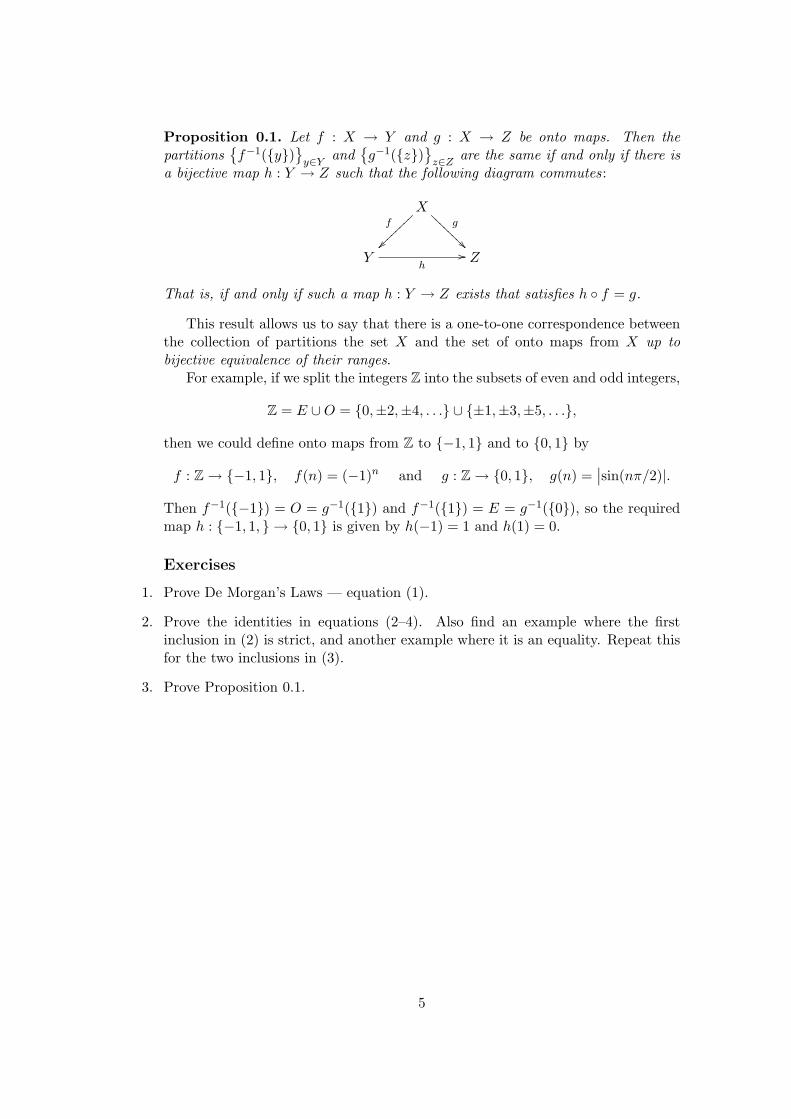
Proposition 0.1. Let f : X → Y and g : X → Z be onto maps. Then thepartitions

{f−1({y})

}y∈Y

and{g−1({z})

}z∈Z

are the same if and only if there isa bijective map h : Y → Z such that the following diagram commutes:

Xf

~~~~~~

~~~~ g

@@@

@@@@

@

Yh

// Z

That is, if and only if such a map h : Y → Z exists that satisfies h ◦ f = g.

This result allows us to say that there is a one-to-one correspondence betweenthe collection of partitions the set X and the set of onto maps from X up tobijective equivalence of their ranges.

For example, if we split the integers Z into the subsets of even and odd integers,

Z = E ∪O = {0,±2,±4, . . .} ∪ {±1,±3,±5, . . .},

then we could define onto maps from Z to {−1, 1} and to {0, 1} by

f : Z → {−1, 1}, f(n) = (−1)n and g : Z → {0, 1}, g(n) =∣∣sin(nπ/2)|.

Then f−1({−1}) = O = g−1({1}) and f−1({1}) = E = g−1({0}), so the requiredmap h : {−1, 1, } → {0, 1} is given by h(−1) = 1 and h(1) = 0.

Exercises

1. Prove De Morgan’s Laws — equation (1).

2. Prove the identities in equations (2–4). Also find an example where the firstinclusion in (2) is strict, and another example where it is an equality. Repeat thisfor the two inclusions in (3).

3. Prove Proposition 0.1.

5

1 Metric Spaces

Definition and examples

Recall what it means for a function f : R → R to be continuous at a point a ∈ R:

∀ε > 0 ∃δ > 0 s.t. |x− a| < δ ⇒ |f(x)− f(a)| < ε

In words this says that for any degree of error ε we can find some positive numberδ such that if x is within distance δ of a then f(x) is less than ε from f(a). Thesame thing is true if we consider a function g : R2 → R; this is continuous at thepoint (a, b) if

∀ε > 0 ∃δ > 0 s.t. |(x, y)− (a, b)| < δ ⇒ |g(x, y)− g(a, b)| < ε

where here |(x, y) − (a, b)| =√

(x− a)2 + (y − b)2 is the Euclidean distance of(x, y) from (a, b). So again we have that g(x, y) will be as close to g(a, b) as welike, provided we take (x, y) sufficiently close to (a, b). The basic idea of a metricspace is to abstract this idea of distance between points in Euclidean space.

Definition 1.1. Let X be a nonempty set. A metric on X is a function d :X ×X → R that satisfies:

M1 d(x, y) ≥ 0 ∀x, y ∈ X, with d(x, y) = 0 if and only if x = y.

M2 d(x, y) = d(y, x) ∀x, y ∈ X. (symmetry)

M3 d(x, y) ≤ d(x, z) + d(z, y) ∀x, y, z ∈ X. (triangle inequality)

The pair (X, d) is called a metric space, and we say that d(x, y) is distance betweenx and y.

Example 1.2.

(a) X = R, the real line, and d(x, y) = |x− y|.

(b) X = C, the complex plane, and d(z, w) = |z − w|.

where in both cases | · | denotes the usual modulus function. In both cases M1 andM2 are easily seen to hold; for (b) note that we have

|z + w| ≤ |z|+ |w| ∀z, w ∈ C,

which is the inequality that is usually referred to as the triangle inequality. Givenany other u ∈ C it follows that

d(z, w) = |z − w| = |(z − u) + (u− w)| ≤ |z − u|+ |u− w| = d(z, u) + d(u, w)

as required. This (partly) explains the terminology of M3. The inequality forexample (a) is verified in the same way.

Thus we see that the properties M1, M2 and M3 hold in R and in C. In factthey continue to hold in Rn for any n when equipped with the usual Euclideandistance, and careful inspection of the proofs of many results about continuousfunctions Rm → Rn show that these are the only properties that are really used.

6

Example 1.3. Consider X = Rn together with the map d2 : X × X → [0,∞)given by

d2

((x1, . . . , xn), (y1, . . . , yn)

)=

√∑ni=1(xi − yi)2.

This defines a metric on Rn (exercise — prove this; M3 requires making use ofthe Cauchy-Schwarz inequality). The pair (Rn, d2) is known as n-dimensionalEuclidean space.

But d2 is by no means the only metric on Rn. Consider instead the metric d1

given byd1

((x1, . . . , xn), (y1, . . . , yn)

)=

∑ni=1 |xi − yi|.

This again is easily seen to be a metric on Rn (indeed, it is simpler to check M3this time), but note that (Rn, d1) 6= (Rn, d2) whenever n > 1. For instance, if wetake x = (0, · · · , 0) and y = (1, · · · , 1) then we get

d1(x,y) = n 6=√

n = d2(x,y).

The last example showed that we have more than one metric on familiar spacessuch as Rn. In fact it is possible to define a metric on any nonempty set.

Example 1.4. Let X be a nonempty set and define d : X ×X → [0,∞) by

d(x, y) =

{0 if x = y,

1 if x 6= y.

Then (X, d) is a metric space in which every point is equidistant from every otherpoint! This metric d is called the discrete metric.

Other natural examples of metrics are those defined on sets of functions.

Example 1.5. Let X = C[0, 1], the set of all continuous functions from [0, 1] to C.This is an infinite dimensional vector space under the pointwise defined operations

(f + g)(x) = f(x) + g(x), (tf)(x) = tf(x).

where f, g ∈ X, 0 ≤ x ≤ 1 and t ∈ C. Define

d1(f, g) =∫ 1

0|f(x)− g(x)| dx.

Then d1 is a metric on X. It obviously satisfies M2, and for M3 we have for anyh ∈ X that

d1(f, g) =∫ 1

0|f(x)− h(x) + h(x)− g(x)| dx

≤∫ 1

0

{|f(x)− h(x)|+ |h(x)− g(x)|

}dx

=∫ 1

0|f(x)− h(x)| dx +

∫ 1

0|h(x)− g(x)| dx

= d1(f, h) + d1(h, g).

7

It is also easy to see that d1(f, g) ≥ 0 for any f, g ∈ X and that d1(f, f) = 0.Exercise: prove carefully that if d1(f, g) = 0 then f = g.

Again, there are other natural metrics on this set X. For instance

d∞(f, g) = sup0≤x≤1

|f(x)− g(x)|

defines a metric on X (prove this!). Again, we have d∞ 6= d1. For instance takef(x) = 0 and g(x) = x2, then we have that

d1(f, g) =∫ 1

0x2 dx = [x3/3]10 = 1/3

and

d∞(f, g) = sup0≤x≤1

x2 = 1.

Note that the modulus function of R defines a metric on the subset Q of rationalnumbers. That is, (Q, | · |) is a metric space. It is incomplete, unlike (R, | · |). Thisis one example of how to make new metric spaces out of others.

Proposition 1.6. (a) Let (X, dX) be a metric space and let Z be any nonemptysubset of X. Let dZ denote the restriction of the function dX to the subset Z × Zof X ×X. Then (Z, dZ) is a metric space.

(b) Let (X, dX) and (Y, dY ) be metric spaces, and let W = X × Y . Then thefollowing are three metrics on W :

d1

((x1, y1), (x2, y2)

)= dX(x1, x2) + dY (y1, y2)

d2

((x1, y1), (x2, y2)

)=

√dX(x1, x2)2 + dY (y1, y2)2

d∞((x1, y1), (x2, y2)

)= max

{dX(x1, x2), dY (y1, y2)

}Proof. Exercise.

The space (Z, dZ) is a subspace of (X, dX). The set W with any of the metricsd1, d2 or d∞ is a candidate for the product of (X, dX) and (Y, dY ), and in a certainsense (W,d1), (W,d2) and (W,d∞) are equivalent as we shall see later. The productconstruction extends the product of any finite number of metric spaces. Productsof an infinite number of spaces require more care.

Convergence and continuity

Analysis is concerned with the study of limits and continuity. Now that we haveintroduced the idea of a metric space with its notion of the distance between anytwo points of an abstract set, we can give the obvious definitions for convergenceof sequences and continuity of functions in this setting.

Definition 1.7. Let (X, dX) and (Y, dY ) be metric spaces, and let x ∈ X.

8

(a) Let (xn)n≥1 be a sequence of elements from X. The sequence converges tox if for each ε > 0 there is some N ≥ 1 such that

n ≥ N ⇒ d(xn, x) < ε

This is denoted limn xn = x or xn → x.

(b) A function f : X → Y is continuous at x0 ∈ X if for each ε > 0 there issome δ > 0 such that

dX(x0, x) < δ ⇒ dY (f(x0), f(x)) < ε.

The function is said to be continuous (on X) if it is continuous at each pointof X.

Note. The sequence (xn) converges to x if and only if dX(xn, x) → 0, where we arenow dealing with the familiar concept of convergence of sequences of real numbers.In particular the above definition coincides with the usual one for sequences ofnumbers, when R is equipped with its usual metric.

Example 1.8. The particular choice of metric can make a big difference as towhether or not a sequence is convergent. For example consider X = C[0, 1] withthe metrics d1 and d∞ as given in Example 1.5, and consider the following sequenceof functions:

1

1

1

1

1

1

f1 f2 f3

1

2

1

3

We have d1(fn, 0) = 12n → 0, and so fn → 0 with respect to d1. However

d∞(fn, 0) = 1 for all n, and so fn 6→ 0 with respect to the uniform metric.On the other hand, let d denote the discrete metric. If (gn) ⊂ C[0, 1] is con-

vergent to some g then there should be some N ≥ 1 such that d(g, gn) < 1 for alln ≥ N . Hence d(g, gn) = 0 for all n ≥ N — the sequence is eventually constant,which is certainly not true of the fn above.

Having introduced a general notion of distance, we want to show that we cando away with this when discussing continuity, rephrasing everything in terms of adistinguished class of subsets. The idea of distance still does have an important(even indispensable) role in other matters.

Definition 1.9. Let (X, d) be a metric space. For any x ∈ X and ε > 0 we write

B(x, ε) = {y ∈ X : d(x, y) < ε}.

The set B(x, ε) is called the open ball of radius ε centred on x.

9

Example 1.10. Equipping R with its usual metric we see that B(x, ε) is the openinterval (x−ε, x+ε). Conversely, if we take any bounded open interval (a, b) thenthis is equal to B(x, ε) for x = (a + b)/2 and ε = (b− a)/2.

Example 1.11. Consider the set X = R2 together with the metrics d1 and d2

from Example 1.3, along with a third metric d∞ given by d∞(x, y) = max{|x1 −y1|, |x2 − y2|} (exercise: check this is a metric). The open balls of radius 1 aboutthe origin 0 have the following forms:

11

1 1 1

1

d1 d2 d3

Example 1.12. If a set X is a given the discrete metric then

B(x, ε) =

{{x} if ε ≤ 1,

X if ε > 1.

Definition 1.13. Let X be a metric space.

(a) A subset U of a metric space X is open (in X) if for each x ∈ U there issome ε > 0 such that B(x, ε) ⊂ U . The ε is allowed to depend on the pointx.

(b) A subset R of X is a neighbourhood of the point x ∈ X if R is an open setsuch that x ∈ R.

PSfrag

R

xε

B(x, ε)

Remarks. (i) It follows vacuously that the empty set ∅ is open — there are nopoints x ∈ ∅ to check.

(ii) Some authors use a slightly more general definition of neighbourhood thatdoes not require R to be an open set. However it should still contain an open ballcentred on x.

The next result shows that all the various notions of open fortunately coincide.

10

Proposition 1.14. Let X be a metric space. Each open ball is an open set ac-cording the above definition.

x

yδ

ε

Proof. Pick an open ball B(x, ε) and a point y ∈ B(x, ε). So in particular we haved(x, y) < ε, hence δ := ε − d(x, y) > 0. Consider the ball B(y, δ). If z ∈ B(y, δ)then

d(x, z) ≤ d(x, y) + d(y, z) < d(x, y) + δ = d(x, y) + ε− d(x, y) = ε.

Thus B(y, δ) ⊂ B(x, ε) as required.

Remark. We have shown that B(x, ε) is a neighbourhood of all of its points.

As an example of a subset of R that is not open, consider [a, b] for any a ≤ b.(In particular we could take a = b = 0 to get the set {0}). Now for any point xsuch that a < x < b we can find some ε > 0 such that (x − ε, x + ε) ⊂ [a, b]. Forexample let ε = min{x−a, b−x}. But no such ε exists for a or b. For example, theset B(a, ε) contains points to the left of a, and consequently outside the interval[a, b]. Similarly at b. For the same sort of reason, neither (a, b] nor [a, b) is open,where now we must take a < b.

Proposition 1.15. Let (X, d) be a metric space, x ∈ X and (xn) a sequence inX. The following are equivalent :

(i) xn → x as n →∞.

(ii) For each neighbourhood R of the point x there is some N ≥ 1 such that

n ≥ N ⇒ xn ∈ R.

[This is written: the sequence (xn) is eventually/ultimately in R]

Proof. (i ⇒ ii): Let R be a neighbourhood of x, so R is an open set such thatx ∈ R. Hence there is some ε > 0 such that B(x, ε) ⊂ R. Now xn → 0, so there issome N ≥ 1 such that

n ≥ N ⇒ xn ∈ B(x, ε) ⊂ R

as required.

11

(ii ⇒ i): Let ε > 0, then B(x, ε) is a neighbourhood of x, and so by definitionthere is some N such that

n ≥ N ⇒ xn ∈ B(x, ε),

that is, xn → x, since ε was arbitrary.

The next result gives several characterisations of continuity at a point, but inorder to state these we must recall the notation given in Section 0 concerning mapsand subsets.

Definition 1.16. Let X and Y be sets and f : X → Y a map. Let A ⊂ X andB ⊂ Y be subsets. Then

f(A) = {f(x) : x ∈ A} (the image of A)

f−1(B) = {x ∈ X : f(x) ∈ B} (the inverse image or preimage of B)

That is, f(A) consists of all those elements of Y that are the image of some pointof A, and f−1(B) consists of all those points of X that are mapped into B.

Note. We do not require f to be surjective, so there could be some points in Bthat no element of X is mapped to. So we could have f−1(B) = ∅ when B 6= ∅ —consider f−1([2, 3]) when f : R → R is the map f(x) = sinx. On the other hand,if A 6= ∅ then f(A) 6= ∅.

Proposition 1.17. Let f : X → Y be a map between metric spaces, and let x ∈ X.The following are equivalent :

(i) f is continuous at x

(ii) For each ε > 0 there is some δ > 0 such that f(B(x, δ)

)⊂ B(f(x), ε).

(iii) For each neighbourhood S of f(x) there is some neighbourhood R of x suchthat f(R) ⊂ S. [i.e. x ∈ R ⇒ f(x) ∈ S]

(iv) If (xn) ⊂ X is any sequence such that xn → x, then f(xn) → f(x).

Proof. The equivalence of (i) and (ii) is clear — we have just rewritten the def-inition of continuity at a point in terms of open balls and their images underf .

(ii ⇒ iii): Let S be any neighbourhood of f(x), so then S is an open set suchthat f(x) ∈ S. Thus there is some ε > 0 such that B(f(x), ε) ⊂ S. Now by (ii) weknow that there is some δ > 0 such that f

(B(x, δ)

)⊂ B(f(x), ε) ⊂ S, and B(x, δ)

is a neighbourhood of x.(iii ⇒ iv): Let (xn) be any sequence that is convergent to x, and let S be any

neighbourhood of f(x). Then there is a neighbourhood R of x such that f(R) ⊂ S.But xn → x, and so there is some N ≥ 1 such that if n ≥ N then xn ∈ R. Butthis implies that

n ≥ N ⇒ xn ∈ R ⇒ f(xn) ∈ f(R) ⊂ S

12

and so f(xn) → f(x) as required, by Proposition 1.15.(iv ⇒ ii): Suppose that (ii) does not hold, so then there must be some ε > 0

such thatf(B(x, δ)) 6⊂ B(f(x), ε) ∀δ > 0.

In particular f(B(x, 1/n)

)6⊂ B(f(x), ε) for each integer n ≥ 1, and so we can

choose xn ∈ B(x, 1/n) for each n such that d(f(x), f(xn)

)≥ ε.

So now (xn) is a sequence in X with d(x, xn) < n−1 → 0, so that xn → x. Butf(xn) 6→ f(x), since d

(f(x), f(xn)

)6→ 0. Hence (iv) does not hold. Taking the

contrapositive gives (iv ⇒ ii) as required.

Corollary 1.18. Let f : X → Y be a map between metric spaces. The followingare equivalent :

(i) f is continuous

(ii) For each open subset V ⊂ Y , f−1(V ) is open in X

Proof. (i ⇒ ii): Suppose V ⊂ Y is open and let x ∈ f−1(V ). Now V is a neigh-bourhood of f(x) and f is continuous at x, so by part (iii) of our proposition thereis some neighbourhood R of x such that f(R) ⊂ V . This implies that R ⊂ f−1(V ).

But R being a neighbourhood of x means that there is some δ > 0 such thatB(x, δ) ⊂ R ⊂ f−1(V ), and so f−1(V ) is open.

(ii ⇒ i): Let x ∈ X and let V ⊂ Y be open with f(x) ∈ V . That is, V is aneighbourhood of f(x), and f−1(V ) is open by hypothesis. Moreover x ∈ f−1(V )and f(f−1(V )) ⊂ V . So f is continuous at x by condition (iii) of the proposition,and since x was arbitrary, f is continuous on X.

Properties of open and closed sets

We have now characterised continuity of maps in terms of the behaviour of aparticular class of subsets under the operation of taking the inverse image. Thiswill be the basis of the definition of continuity later on in the context of topologicalspaces. First we must investigate other useful properties of open sets, since thiswill also inform these later definitions.

Proposition 1.19. Let X be a metric space. The subsets X and ∅ are open.Moreover :

(a) If {Uλ}λ∈Λ is a family of open subsets of X then their union⋃

λ∈Λ Uλ is alsoopen.

(b) If {Vi}ni=1 is a finite family of open subsets of X then their intersection⋂n

i=1 Vi is again open.

Proof. Let x ∈ X then B(x, ε) ⊂ X for all choices of ε > 0, hence X is open.Similarly, to show ∅ is open we must find, for any given x ∈ ∅, an ε > 0 such thatB(x, ε) ⊂ ∅. But this holds vacuously, since there are no points in ∅!

(a) Let x ∈⋃

λ Uλ, then x ∈ Uλ0 for some λ0 ∈ Λ, the indexing set. Now Uλ0

is open and so there is some ε > 0 such that B(x, ε) ⊂ Uλ0 ⊂⋃

λ Uλ. Hence theunion is open.

13

(b) It is enough to prove this for the intersection of two open sets, U and Vsay, since the general case then follows by induction. So let x ∈ U ∩V , then x ∈ Uand x ∈ V , and thus there are numbers εU > 0 and εV > 0 such that

B(x, εU ) ⊂ U and B(x, εV ) ⊂ V.

Put ε = min{εU , εV }, then ε > 0 and

B(x, ε) = B(x, εU ) ∩ B(x, εV ) ⊂ U ∩ V,

and so U ∩ V is open.

Remarks. (i) In part (a) the family {Uλ}λ∈Λ may contain an uncountable numberof sets. One way to think of this object is as a map from the index set Λ into thepower set P(X), whose range lies in the subclass of open sets.

(ii) Part (b) already begins to fail if we take the intersection of a countablefamily of open sets. For example take a ≤ b in R and for each n ≥ 1 consider theopen interval

Un = (a− 1/n, b + 1/n).

These are all open (they are open balls), but⋂n≥1Un = [a, b]

which is not open.Although we shall generally define everything in terms of open sets in what

follows, an alternative ‘dual’ point of view is available, produced by taking thecomplement of everything in sight.

Definition 1.20. Let X be a metric space. A subset F ⊂ X is closed if F c = X\Fis open.

Taking the complement of Proposition 1.19 and applying De Morgan’s Lawsyields:

Proposition 1.21. The intersection of any family of closed sets is again closed.The union of a finite number of closed sets is again closed.

Proof. If {Fλ}λ∈Λ are closed then

X \⋂

λ Fλ =⋃

λ(X \ Fλ),

a union of open sets, hence open. The second part is proved similarly.

It is important to note that there are sets that are both open and closed, andsome that are neither. Indeed in any metric space X the sets X and ∅ are bothopen and closed, and in many important examples they are the only two sets withthat property. Other examples of closed sets include the closed subintervals of R,that is, sets of the form [a, b] for a ≤ b. That these sets are closed follows since

[a, b]c = (−∞, a) ∪ (b,∞).

That is, the complement is the union of two open sets, so is itself open. Examplesof sets that are neither open nor closed are the intervals (a, b] and [a, b) (wherenow we must take a < b to avoid obtaining the empty set).

14

Definition 1.22. Let X be a metric space and A ⊂ X a subset. The closure ofA, denoted A, is the smallest closed subset of X that contains A.

To see that this definition actually makes sense, consider the following familyof sets:

F = {F ⊂ X : F closed, F ⊃ A}.

Note that X ∈ F , no matter what choice of A we take, so the family F is nonempty.Put A1 =

⋂F∈F F , then A1 is closed by Proposition 1.21. Moreover, since A ⊂ F

for all F ∈ F , we have A ⊂ A1. Conversely if E is any closed set that contains Athen E ∈ F and so A1 ⊂ E by construction of A1. Thus A1 is the smallest closedset containing A.

Proposition 1.23. Let A be a subset of a metric space X, and let x ∈ X. Thefollowing are equivalent :

(i) x ∈ A.

(ii) R ∩A 6= ∅ for all neighbourhoods R of x.

(iii) x = limn xn for some sequence (xn) ⊂ A.

Proof. (i ⇒ ii): Suppose for a contradiction that there is some neighbourhood Rof x that satisfies R ∩ A = ∅. Then A ⊂ Rc, and Rc is closed since R is open.Then, by definition of A,

A ⊂ Rc ⇒ A ⊂ Rc ⇒ A ∩R = ∅.

Since x ∈ R we get x /∈ A, the required contradiction.(ii ⇒ iii): For each integer n ≥ 1 we can take R = B(x, 1/n), and thus pick

some xn ∈ B(x, 1/n) ∩ A. Then (xn) ⊂ A, and d(x, xn) < 1/n for all n. Hence(xn) ⊂ A and xn → x.

(iii ⇒ i): Suppose that x = limn xn for some sequence (xn) ⊂ A, but thatx /∈ A. Then x ∈ A

c, and Ac is open, hence a neighbourhood of x. But then,

by Proposition 1.15, we have xn ∈ Ac for all sufficiently large n, so that xn /∈ A,

hence xn /∈ A, which is impossible. Thus, by contradiction, x ∈ A.

Note that by definition A is closed, so if A ⊂ X satisfies A = A then it is aclosed subset. On the other hand, if A is known to be closed then it is clearly thesmallest closed subset that contains itself, and so A = A. That is, A = A if andonly if A is closed. In particular, since A is closed, the closure of the closure isjust A, that is A = A.

Corollary 1.24. Let A be a subset of a metric space X. Then A is closed if andonly if limn xn ∈ A for every sequence (xn) ⊂ A that is convergent in X.

Proposition 1.25. Let X be a metric space.

(a) For any collection {Aλ}λ∈Λ of subsets of X we have⋂λ Aλ ⊂

⋂λ Aλ.

15

(b) For any finite collection {Bi}ni=1 of subsets of X we have⋃

i Bi =⋃

i Bi.

Proof. (a) Since Aλ ⊂ Aλ for all λ ∈ Λ we have⋂λ Aλ ⊂

⋂λ Aλ.

But the set on the right hand side is closed by Proposition 1.21, so by definition⋂λ Aλ ⊂

⋂λ Aλ.

(b) Similar reasoning gives ⋃i Bi ⊂

⋃i Bi

since our union is finite. So let x ∈⋃

i Bi, then x ∈ Bj for some 1 ≤ j ≤ n. Thus

(R ∩Bj) 6= ∅

for all neighbourhoods R of x, and consequently,

R ∩Bj ⊂⋃

i(R ∩Bi) = (R ∩⋃

i Bi) 6= ∅

for every such R. Hence x ∈⋃

i Bi as required.

It is impossible to get equality in (a) in general, even if we restrict ourselvesto only a finite number of sets. For examples consider the subsets A = (0, 1) andB = (1, 2) of R. Then

A ∩B = ∅ ⇒ A ∩B = ∅; A = [0, 1], B = [1, 2] ⇒ A ∩B = {1}.

Similarly we must take a finite number of sets in (b); again working with subsetsof R we put Bq = {q} for each q ∈ Q, then Bq = {q}, and so⋃

q∈Q Bq = Q, but⋃

q∈Q Bq = Q = R.

Exercises

1. (a) Prove that the following inequality holds for any n ≥ 1 and ai, bi ∈ [0,∞):∑ni=1 aibi ≤

(∑ni=1 a2

i

)1/2(∑ni=1 b2

i

)1/2 (‡)

[Hint: consider the quadratic polynomial p(x) =∑

i(ai − xbi)2.]Hence show that the map d2 defined as follows is a metric on Cn

d2

((z1, . . . , zn), (w1, . . . , wn)

)=

(∑ni=1 |zi − wi|2

)1/2

16

(b) Prove that if f : [0, 1] → [0,∞) is a continuous function then∫ 1

0f(t) dt = 0 ⇔ f(t) = 0 ∀t ∈ [0, 1].

Hence show that the map d1 defined as follows is a metric on C[0, 1]

d1(f, g) =∫ 1

0|f(t)− g(t)| dt

[To show that the function d2(f, g) =(∫ 1

0 |f(t)− g(t)| dt)1/2

is a metric on C[0, 1]requires an analogue of (‡).]

2. Find three different metrics on N, no two of which are multiples of each other.

3. Let (X, d) be a metric space. Show that d′ defined by

d′(x, y) =d(x, y)

1 + d(x, y)

is another metric on X. [Note that d′(x, y) < 1 ∀x, y ∈ X.]

4. Consider the function d : R2 × R2 → R defined by

d((x1, y1), (x2, y2)

)=

{|y1 − y2| if x1 = x2,

|y1|+ |x1 − x2|+ |y2| if x1 6= x2.

Show that d is a metric on R2. Sketch the balls B((2, 0), 1

), B

((1, 2), 1

)and

B((1, 1), 2

).

5. Let X be a set and d a map X ×X → R satisfying

M1′ d(x, y) = 0 ⇔ x = y, and M2′ d(x, y) ≤ d(x, z) + d(y, z) ∀x, y, z ∈ X.

Show that d is a metric on X.

6. Let (xn) and (yn) be two convergent sequences in a metric space X, with x =limn xn and y = limn yn. Show that d(xn, yn) → d(x, y).

7. Let X be a metric space and let f : X → R and g : X → R continuous functions.Show that f + g, tf (t ∈ R), |f |, max{f, g}, min{f, g} and fg are continuous,where

(f + g)(x) = f(x) + g(x), (tf)(x) = tf(x), |f |(x) = |f(x)|, etc.

8. Let X = C[0, 1] and let F : X → C denote the map F (f) = f(0) (for f ∈ X). IsF continuous when X is given (i) the d1 metric, or (ii) the d∞ metric?

9. Show that any open set in R (with the usual metric) is the union of a countablecollection of open intervals. Show that this collection can be chosen so that anytwo distinct intervals are disjoint.

17

10. Prove that the set {x} is closed for any point x in any metric space X.

11. Prove that a subset of a metric space is open if and only if it is a union of openballs.

12. Prove that every subset of a discrete metric space X is open. Hence show thatany map f : X → Y from X into any other metric space Y is continuous.

13. We have shown that a function f : X → Y between metric spaces is continuous ifand only if for every open set U in Y , the set f−1(U) is open in X. The analogousstatement involving images does not hold: find an example of metric spaces X andY and a continuous map f : X → Y such that f(V ) is not open for some open setV ⊂ X.

14. Prove that Q ∩ (x, x + ε) 6= ∅ for all choices of x ∈ R and ε > 0. Hence deducethat the closure of Q is R.

15. Let A be a subset of a metric space X. Show that if x ∈ A \ A then each openball centred on x contains an infinite number of (distinct) points of A. Does thisremain true if we take x ∈ A?

16. Let X and Y be metric spaces, and A a subset of X. If f : X → Y and g : X → Yare continuous functions such that f(x) = g(x) for all x ∈ A, show that f(x) = g(x)for all x ∈ A.

17. Let d1, d2 and d∞ be the metrics on R2 given by

d1

((x1, x2), (y1, y2)

)= |x1 − y1|+ |x2 − y2|,

d2

((x1, x2), (y1, y2)

)=

{|x1 − y1|2 + |x2 − y2|2

}1/2,

d∞((x1, x2), (y1, y2)

)= max

{|x1 − y1|, |x2 − y2|

}.

Show that these metrics are Lipschitz equivalent. Show that the discrete metricon R2 is not Lipschitz equivalent to any of the above metrics.

18. Prove that the metric d1 on C[0, 1] is not Lipschitz equivalent to the metric d∞,where d∞(f, g) = supt∈[0,1] |f(t)− g(t)|.

18

2 Topological Spaces

Definitions and examples

Having had a brief excursion through metric space theory, we have prepared theway for a further generalisation, where now we can consider the theory of topo-logical spaces. The idea is to do away totally with the concept of distance, anddeal only with subsets of our space.

Definition 2.1. A topological space is a pair (X, T) consisting of a nonemptyset X and a collection T of subsets of X that satisfy the following properties:

T1 ∅, X ∈ T

T2 If {Uλ}λ∈Λ ⊂ T, then⋃

λ Uλ ∈ T.

T3 If {Vi}ni=1 ⊂ T then

⋂i Vi ∈ T.

The collection T is called a topology, and its elements of are called open sets.The axioms state that the union of any collection of open sets is again open, butwe only require that T be closed under finite intersections.

So note that here we are supplied with our open sets, whereas in the case ofmetric spaces it was the metric that was fundamental, and with which we had tocheck if a given set was open or not.

Example 2.2. The following are all examples of topological spaces:

(i) The indiscrete topology on any (nonempty) set X is the collection {∅, X}.

(ii) The discrete topology on any (nonempty) set X is the power set P(X)consisting of all subsets of X.

(iii) If (X, d) is a metric space, then let Td denoted the collection of subsets thatare open with respect to d, as in Definition 1.13. Then the pair (X, Td) is atopological space by Proposition 1.19.

If (Y, T) is a topological space for which there is some metric d on Y such thatT = Td, then the space (Y, T) is said to be metrizable. Not all topologicalspaces occur this way — for example if |X| ≥ 2 then X equipped with theindiscrete topology is not metrizable (why?). On the other hand, the discretetopology is that induced by the discrete metric.

(iv) Given a set X, the cofinite or Zariski topology on X consists of ∅ togetherwith any subset A such that Ac = X \ A is finite. Exercise: show that thisdoes indeed define a topology on X.

Again, this is (rarely) a metrizable topological space, but is of great impor-tance in algebraic topology since it is well-suited for the study of polynomialequations. The Zariski topology on C has far fewer open sets than in theusual metric topology. In fact, the only closed sets are those correspondingto the zeros of polynomials.

19

Definition 2.3. Let (X, T) and (Y,S) be topological spaces, and let f : X → Ybe a map. Then f is continuous if

V ∈ S ⇒ f−1(V ) ∈ T.

If we want to stress the topologies involved, we say that f is (T,S)-continuous.

Again, we should check that we have not lost anything from metric space duringthis process of generalisation. That is, if f : X → Y is a map between metric spaces(X, dX) and (Y, dY ) then we would like it to be continuous according to the metricspace definition (Definition 1.7) if and only if it continuous with respect to thetopological space definition, where we equip X and Y with the topologies inducedby their metrics. But this is essentially the content of Corollary 1.18.

Also, we are now finally in a position to explain why the choice of metric issometimes not all that important.

Definition 2.4. Let X be a nonempty set, and let d1 and d2 be metrics on X.They are Lipschitz equivalent if there are constants 0 < a ≤ b such that

ad1(x, y) ≤ d2(x, y) ≤ bd1(x, y) ∀x, y ∈ X.

Examples of metrics that satisfy this condition include d1, d2 and d∞ on Rn

as defined in Example 1.3 and Example 1.11. One can check that

d∞(x,y) ≤ d1(x,y) ≤√

nd2(x,y) ≤ nd∞(x,y),

where the second inequality follows by an application of the Cauchy-Schwarz in-equality.

Whenever we have Lipschitz equivalent metrics, we end up in the followingpleasant situation:

Proposition 2.5. Let X be a nonempty set, and let d1 and d2 be metrics on Xthat are Lipschitz equivalent. Then the topologies that they induce on X are thesame. Consequently if (Y, d) is any other metric space, and g any map X → Yor Y → X, then g is continuous with respect to the d1 metric if and only if it iscontinuous with respect to the d2 metric.

Proof. This follows from the inclusions

B1(x, δ/b) ⊂ B2(x, δ) and B2(x, ε/a) ⊂ B1(x, ε)

Thus in many ways it is unimportant which metric we choose to work withwhen dealing with Rn (or any subset of Rn), and so we can choose whicheveris most convenient at that particular instant. Similar arguments show that thethree metrics given on the product X × Y of two metric spaces are also Lipschitzequivalent, and hence lead to the same topology.

As an example of the economy gained by generalising to topological spaces, anddealing with global rather than local continuity, considering the following resultthat is standard in any course on real or complex analysis:

20

Proposition 2.6. Let (Xi,Ti), i = 1, 2, 3 be topological spaces, and let f : X1 →X2 and g : X2 → X3 be continuous maps. Then their composition g ◦f : X1 → X3

is continuous.

Proof. For any subset A ⊂ X3 we have (g ◦ f)−1(A) = f−1(g−1(A)), and so

U ∈ T3 ⇒ g−1(U) ∈ T2 ⇒ f−1(g−1(U)) = (g ◦ f)−1(U) ∈ T1,

since f and g are continuous. Hence g ◦ f is continuous.

Definition 2.7. Let (X, T) be a topological space. A subset F ⊂ X is closed ifF c = X \ F ∈ T.

Note that this is precisely the same definition as given in the special case ofmetric spaces. So X and ∅ are closed, and once again, De Morgan’s laws leadimmediately to:

Proposition 2.8. The intersection of any family of closed sets in a topologicalspace is closed. The union of any finite number of closed sets is closed.

Topology can be developed in terms of closed rather than open sets, as thefollowing shows:

Proposition 2.9. Let f : X → Y be a map between topological spaces. Then f iscontinuous if and only if for every closed subset F ⊂ Y , f−1(F ) is closed in X.

Proof. This is an immediate consequence of the following identity:

f−1(Y \A) = X \ f−1(A),

which is valid for any subset A ⊂ Y .

Thus continuity could have instead been defined by saying that the inverseimage of any closed subset is closed, rather than the given definition.

Sequences; separation axioms

The concepts of convergence of sequences, and of closure of sets carries over, ifwe think about them in the correct way. For convergence of sequences we mustnow make use of the alternative characterisation of convergence given in Proposi-tion 1.15, since we no longer have any open balls to hand.

Definition 2.10. Let (xn) be a sequence in a topological space X, and let x ∈ X.Then the sequence converges to x if for every neighbourhood R of x there is someN ≥ 1 such that

n ≥ N ⇒ xn ∈ R.

At this point where we can illustrate one way in which topological spaces canbe very far from our intuitive ideas coming from metric space theory. If X is anyset equipped with the indiscrete topology, then every sequence in X converges toevery point of X. This happens because T = {∅, X}, so given any x ∈ X and(xn) ⊂ X, the only open set containing x is X itself, and xn ∈ X for all n!

21

One way to avoid this embarrassment is to impose a further condition on thesort of topologies that we shall work with. Such conditions fall under the headingof separation axioms and involve making use of open sets to distinguish betweenpoints. One of the most important examples is the following:

Definition 2.11. A Hausdorff space is any topological space (X, T) such that ifx, y ∈ X with x 6= y, then there are U, V ∈ T such that

x ∈ U, y ∈ V and U ∩ V = ∅.

That is, there are neighbourhoods of x and y that are disjoint.

One way of remembering what the Hausdorff condition does for you, is that“distinct points can be housed off.” There are weaker conditions than this (e.g.T1-spaces) and stronger conditions (e.g. normal spaces). Simmons has more infor-mation on these. One useful effect of restricting our attention to Hausdorff spacesis that sequences are better behaved.

Proposition 2.12. Any sequence in a Hausdorff space has at most one limit.

Proof. Suppose that X is a Hausdorff space and that (xn) is a sequence in Xthat converges to both x and y, with x 6= y. The Hausdorff condition implies theexistence of open sets U and V such that

x ∈ U, y ∈ V and U ∩ V = ∅.

But since xn → x and xn → y we have that the sequence must eventually be inU , as well as eventually being in V , which is impossible.

The reason why we had not encountered such problems earlier is that thetopology induced by a metric automatically makes the space into a Hausdorff space.(Exercise: prove this.) In certain books the authors will assume Hausdorff as partof the definition of a topological space, in order to circumvent such pathologies aswe encountered above. But topologies such as the Zariski topology on an infiniteset are not Hausdorff (and hence cannot be metrizable), and yet have uses inapplications of this general theory.

Now turning to the concept of closures, the following is (almost) word for wordthe same as Definition 1.22.

Definition 2.13. Let X be a topological space and A ⊂ X a subset. The closureof A, denoted A, is the smallest closed subset of X that contains A.

Again to construct A it is enough to take the intersection of all closed subsetsthat contain A. In Proposition 1.23 we characterised the elements of A in twoways, one involving sequences, the other neighbourhoods and their intersectionwith A. The following remains true:

Proposition 2.14. Let A be a subset of a topological space X, and let x ∈ X.Then x ∈ A if and only if R ∩A 6= ∅ for all neighbourhoods R of X.

We have already seen sequences behaving badly once. The next example showsthat we cannot use them to characterise the elements of closures:

22

Example 2.15. Let X = [0, 1] and let T be the family of subsets consisting of∅ together with every subset U such that U c is countable. (Exercise: prove thatthis Zariski-like collection of subsets is indeed a topology, sometimes called thecocountable topology.) Now consider the set A = [0, 1), then we must have

A = [0, 1) or A = [0, 1]

since we always have A ⊂ A. However if A = [0, 1) then Ac = {1} should be open,

and so A = (Ac)c = [0, 1) must be countable. This certainly is not the case, so infact we must have that A = [0, 1].

Now let (an) be any sequence in A, and set U = X \{a1, a2, . . .}. By construc-tion this U is an open set, being the complement of a countable set, and moreover1 ∈ U , since we have only taken out elements of A. But now we see that an 6→ 1,since it never gets into this particular neighbourhood of the point 1 ∈ A. So nosequence from A converges to 1.

Definition 2.16. A subset A of a topological space X is dense if A = X. Atopological space is separable if it has a countable dense subset.

Example 2.17.(i) We have shown previously that Q = R, when R is given its usual topology.

Thus R is separable since Q is a countable dense subset.

(ii) If a nonempty set X is given the indiscrete topology then the closure of anynonempty subset A is the whole space X, since the only closed sets are ∅and X. Thus in particular we have {x} = X for any x ∈ X, and so X isseparable.

(iii) If a nonempty set X is given the discrete topology then every set is open,hence every set is also closed, and so A = A for every subset A ⊂ X. Inparticular the only dense subset of X is X itself. Thus if we equip R withthe discrete topology then it is a nonseparable space.

We can equip a given set X with many different topologies in general. For in-stance we always have the discrete and indiscrete topologies, and these are distinctunless |X| = 1. If T1 and T2 are topologies on the given set X, we say that T1 isweaker or coarser than T2 if T1 ⊂ T2. That is, every set that is T1-open is alsoT2-open. Alternatively T2 is described as being stronger or finer than T1. As anexample, the indiscrete topology is always coarser than the discrete topology.

If T1 and T2 are topologies on X that are related in this way, if (Y, S) is anothertopological space and if f : X → Y is a map, then f is continuous with respect toT2 if it is continuous with respect to T1. Similarly if a given map g : Y → X iscontinuous with respect to T2 then it is continuous with respect to T1. That is,strengthening the topology of the domain/source space does not disrupt continuity,nor does weakening the topology of the codomain/target space.

For example, consider any set X equipped with a topology T, and let Ti andTd denote the indiscrete topologies respectively. Now if we denote the identitymapping X → X by i (that is i(x) = x), then i is always (T,T)-continuous, sincei−1(A) = A for all A ⊂ X, so in particular if A ∈ T then i−1(A) ∈ T. We alsohave that i is

23

• (T,Ti)-continuous,

• (Td,T)-continuous, and

• (Td,Ti)-continuous,

• but not (Ti,Td)-continuous (unless |X| = 1).

Note also that if {Tλ}λ∈Λ is any family of topologies on a set X, then so istheir intersection

⋂λ∈Λ Tλ — this collection will always contain X and ∅.

Subspaces and product spaces

Common ways of creating new topological spaces from old are to restrict to asubset, or take the Cartesian product of two or more, in much the same way as wedid with metric spaces.

Definition 2.18. Let (X, T) be a topological space, and let Z be a nonemptysubset of X. Then TZ = {U ∩ Z : U ∈ T} defines a topology on Z called thesubspace topology, or induced topology.

Obviously one should check that TZ does indeed define a topology on Z. More-over if X is a metric space, then one should check that the topology induced on Zby the metric restricted to Z is the same thing as the subspace topology comingfrom the topology induced by the metric on X. That is, it doesn’t matter whichway we go round the following square:

(X, dX) restrict //

induce

�� $$

(Z, dZ)

induce

��(X, TdX

)restrict

// (Z,TdZ)

This induced topology can be singled out as the only one that has certain niceproperties when it comes to composition of maps.

Proposition 2.19. Let Z be a subset of a topological space (X, T), equip Z withthe subspace topology TZ , and let i denote the inclusion map i : Z ↪→ X that mapsx ∈ Z to x ∈ X. Then for any other topological space (Y, S)

(a) If f : X → Y is continuous, so is f ◦ i : Z → Y .

(b) A map g : Y → Z is continuous if and only if i ◦ g : Y → X is continuous.

Moreover, TZ is the unique topology such that property (b) holds for all choices ofY and g.

24

Proof. For any subset A ⊂ X we have i−1(A) = A ∩ Z, and so if U ∈ T theni−1(U) = U ∩ Z ∈ TZ . In particular i is continuous.

If f : X → Y is a continuous map then f◦i is the composition of two continuousfunctions, and hence also continuous. Similarly if g : Y → Z is continuous. Sosuppose now that g : Y → Z is a map such that i ◦ g is continuous. Then for allU ∈ T we have

g−1(U ∩ Z) = g−1(i−1(U)) = (i ◦ g)−1(U) ∈ S,

and hence g is continuous, since every open subset of Z is of the form U ∩ Z forsome U ∈ T.

Finally, suppose that T1 is a topology on Z such that (b) holds for all choicesof Y and g. Consider the following diagram:

(Y, S)g //

i◦g $$IIIIIIIII

(Z,T1)

izzttttttttt

(X, T)

This must commute whenever we choose (Y,S) and g such that either g is continu-ous or i◦g is continuous. We do this in two different ways, first with Y = Z, S = T1

and g = id. In this case we have that g is continuous, and so i◦g = i is continuousfrom (Z,T1) to (X, T). Hence for any U ∈ T we have that i−1(U) = U ∩ Z ∈ T1.But this says that TZ ⊂ T1, that is TZ is weaker than T1.

Now take Y = Z and g = id again, but instead take S = TZ . This timei ◦ g = i : (Z,TZ) → (X, T), which we have already shown is continuous, hence wemust have that g is continuous. So for each U ∈ T1, g−1(U) = U ∈ TZ , that is,T1 ⊂ TZ . Thus T1 = TZ as required.

We shall now turn to a consideration of product spaces. Consider a curve inR2, which can be thought of as a map f : R → R2 (f might possibly be definedon some subinterval of R). Our work on metric spaces has given us a number ofmetrics on R2 that all lead to the same topology, and in this way we can specifywhether or not the curve is continuous. Alternatively we can always decomposethe map into components:

f(t) =(x(t), y(t)

),

where x and y are now functions R → R. Naively we expect the curve to becontinuous if and only if these component functions are continuous.

If we now turn to abstract sets X1 and X2, and write X = X1 × X2, thenwe can define the coordinate projections pi : X → Xi by pi(x1, x2) = xi. Then,given any other set Y , any map f : Y → X determines two maps pi ◦ f : Y → Xi,and conversely any two maps fi : Y → Xi give a map f : Y → X throughf(y) =

(f1(y), f2(y)

). If we have topologies on X1 and X2, we would like to put

a topology on the product X such that for any other topological space (Y, S), amap f : Y → X is continuous if and only if both the component maps pi ◦ f arecontinuous.

25

Definition 2.20. Let (X1,T1) and (X2,T2) be topological spaces, and let X =X1 ×X2. The product topology T on X is the following collection of sets:

T = {U ⊂ X : for each (x1, x2) ∈ U, there Ui ∈ Ti such thatx1 ∈ U1, x2 ∈ U2 and U1 × U2 ⊂ U}

In particular T contains all sets of the form U1×U2 for Ui ∈ Ti, but also more— see the remark below. To see that the above definition makes sense, we mustdo the following:

Lemma 2.21. The collection T defined above is indeed a topology on X.

Proof. Now X = X1 × X2 by definition, and Xi ∈ Ti for i = 1, 2, from which itfollows that X ∈ T. Similarly, ∅ ∈ T, since it satisfies conditions in the definitionvacuously.

Let {Uλ}λ∈Λ be any family of subsets from T and let (x1, x2) ∈⋃

λ UΛ. Then(x1, x2) ∈ Uλ0 for some λ0 ∈ I. Hence there are Vi ∈ Ti such that

x1 ∈ V1, x2 ∈ V2 and V1 × V2 ⊂ Uλ0 ⊂⋃

λUλ.

and so this union lies in T.Finally, let U, V ∈ T and let (x1, x2) ∈ U ∩ V . Then we can find Ui, Vi ∈ Ti

(i = 1, 2) such that

xi ∈ Ui, xi ∈ Vi, and U1 × U2 ⊂ U, V1 × V2 ⊂ V.

But Ui ∩ Vi ∈ Ti and xi ∈ Ui ∩ Vi for i = 1, 2, and moreover

(x1, x2) ∈ (U1 ∩ V1)× (U2 ∩ V2) = (U1 × U2) ∩ (V1 × V2) ⊂ U ∩ V.

Thus U ∩ V ∈ T.

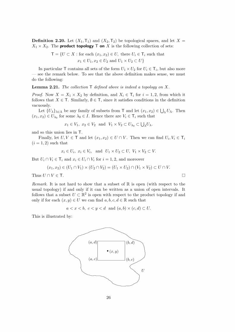
Remark. It is not hard to show that a subset of R is open (with respect to theusual topology) if and only if it can be written as a union of open intervals. Itfollows that a subset U ⊂ R2 is open with respect to the product topology if andonly if for each (x, y) ∈ U we can find a, b, c, d ∈ R such that

a < x < b, c < y < d and (a, b)× (c, d) ⊂ U.

This is illustrated by:

U

(x, y)

(a, c)

(a, d)

(b, c)

(b, d)

26

Sets of the form (a, b)× (c, d) are known as open rectangles (or open boxes,especially in higher dimension). If we set

ε = min{x− a, b− x, y − c, d− y} > 0

then B∞((x, y), ε

)⊂ U , where B∞ denotes the open ball defined with respect

to the d∞ metric, which is Lipschitz equivalent to the metrics d1 and d2 fromExample 1.3. It follows that these three metrics all induce the same topology onR2, which coincides with the product topology.

It is important to note that there are open sets in R2 that are not open rectan-gles, or indeed of the form U1 × U2. The sets of this form are only a basis for thetopology on R2. For instance it is not hard to show that the open ball B(0, 1) ofradius 1 centred on the origin cannot be written as U1 × U2 for open sets Ui ⊂ R

Although the sets in T include things other than (generalised) open boxes, wecan usefully characterise the open sets in terms of these simple products:

Lemma 2.22. Let X1, X2 and X be as above, then any U ∈ T is a union of setsof the form U1 × U2 for Ui ∈ Ti.

Proof. Let U ∈ T, then for each x = (x1, x2) ∈ U we can find Ux ∈ T1 and Vx ∈ T2

such thatx1 ∈ Ux, x2 ∈ Vx and Ux × Vx ⊂ U.

In now follows thatU =

⋃x∈U (Ux × Vx)

as required.

Corollary 2.23. Let X1, X2 and X be as above, let (Y, S) be another topologicalspace, and consider a map f : Y → X. Then f is continuous if and only iff−1(U1 × U2) ∈ S for all Ui ∈ Ti.

Proof. If U ⊂ X is open then it can be written as U =⋃

λ Uλ × Vλ for families{Uλ} ⊂ T1 and {Vλ} ⊂ T2. The result now follows since

f−1(⋃

λ Uλ × Vλ

)=

⋃λ f−1(Uλ × Vλ)

The product topology is set up in such a way that the projections pi arecontinuous, and also so that we use them to characterise continuity of maps fromany other topological space into X.

Lemma 2.24. Let X1, X2 and X be as above. The projections pi : X → Xi arecontinuous.

Proof. This follows since if U1 ∈ T1 then p−11 (U1) = U1 ×X2 ∈ T.

Proposition 2.25. Let X1, X2 and X be as above, let (Y, S) be another topologicalspace and let f : Y → X be a map. Then f is continuous if and only if the mapspi ◦ f : Y → Xi are continuous.

27

Proof. If f is continuous then the maps pi◦f are compositions of continuous maps,hence continuous. So suppose instead that f is a map for which the componentmaps pi ◦f are continuous. To show that f is continuous it is enough to show thatf−1(U1 × U2) ∈ S for any Ui ∈ Ti by Corollary 2.23. But

y ∈ f−1(U1 × U2) ⇔ f(y) ∈ U1 × U2

⇔ (p1 ◦ f)(y) ∈ U1 and (p2 ◦ f)(y) ∈ U2

⇔ y ∈ (p1 ◦ f)−1(U1) ∩ (p2 ◦ f)−1(U2).

That is,

f−1(U1 × U2) = (p1 ◦ f)−1(U1) ∩ (p2 ◦ f)−1(U2).

Continuity of the component functions pi ◦ f implies that (p1 ◦ f)−1(U1) ∈ S and(p2 ◦ f)−1(U2) ∈ S, and so we are done.

A commutative diagram for the above would be the following:

X1

Yf //

p1◦f22

p2◦f ,,

X = X1 ×X2

p1

OO

p2

��X2

As with the subspace topology, it can be shown that the product topology isthe only one for which Proposition 2.25 holds for all choices of space (Y, S) andmap f . Perhaps more important to mention at this juncture is that the aboveprocedure clearly extends products of any finite number of topological spaces. Infact it extends further: let {(Xλ,Tλ)}i∈I be any family of topological spaces, thenX =

∏λ∈Λ Xλ as a set is defined to be the set of maps f : Λ →

⋃λ Xλ such that

f(λ) ∈ Xλ for each λ, and for each λ ∈ Λ the map pλ : X → Xλ is defined bysetting pλ(f) = f(λ). The space X is then equipped with the weakest topology Tsuch that all of the pλ are continuous. [Note, if X is given the discrete topologythen all of the pλ are automatically continuous, hence the set of topologies forwhich the projections are continuous is nonempty. To get T take the intersectionof all the topologies that have this property.] This definition coincides with theone given above when |Λ| = 2.

Quotient spaces; homeomorphisms

Consider a sheet of paper. If it is square we can think of it as the subset [0, 1]×[0, 1]of the plane. If it is rectangular then we should first scale one of the sides to makeit the same length as the other. If we now stick one edge to its opposite edge,

28

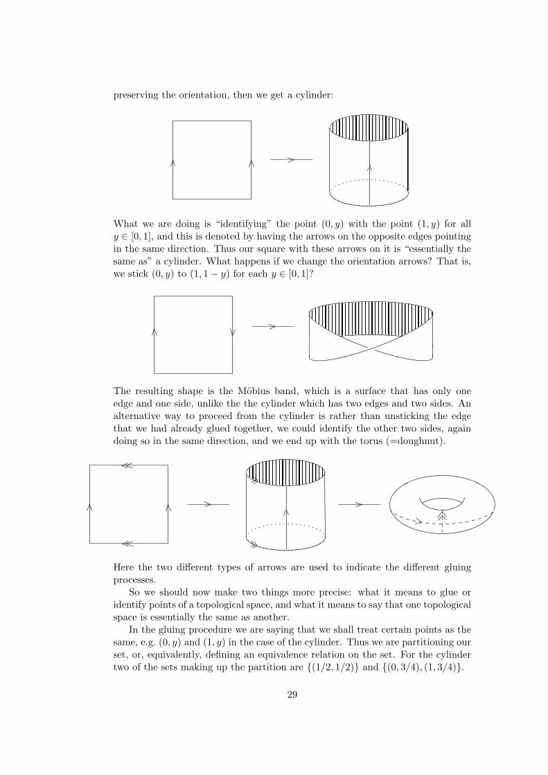
preserving the orientation, then we get a cylinder:

� � � � � � � � � � � �� � � � � � � � � � � �

� � � � � � � � � � � �� � � � � � � � � � � �

What we are doing is “identifying” the point (0, y) with the point (1, y) for ally ∈ [0, 1], and this is denoted by having the arrows on the opposite edges pointingin the same direction. Thus our square with these arrows on it is “essentially thesame as” a cylinder. What happens if we change the orientation arrows? That is,we stick (0, y) to (1, 1− y) for each y ∈ [0, 1]?

����

� � � � � � � � � � � � � � � � � � �� � � � � � � � � � � � � � � � � � �� � � � � � � � � � � � � � � � � � �� � � � � � � � � � � � � � � � � � �

� � � � � � � � � � � � � � � � � � �� � � � � � � � � � � � � � � � � � �� � � � � � � � � � � � � � � � � � �� � � � � � � � � � � � � � � � � � �

The resulting shape is the Mobius band, which is a surface that has only oneedge and one side, unlike the the cylinder which has two edges and two sides. Analternative way to proceed from the cylinder is rather than unsticking the edgethat we had already glued together, we could identify the other two sides, againdoing so in the same direction, and we end up with the torus (=doughnut).

� � � � � � � � � � � �� � � � � � � � � � � �

� � � � � � � � � � � �� � � � � � � � � � � �

Here the two different types of arrows are used to indicate the different gluingprocesses.

So we should now make two things more precise: what it means to glue oridentify points of a topological space, and what it means to say that one topologicalspace is essentially the same as another.

In the gluing procedure we are saying that we shall treat certain points as thesame, e.g. (0, y) and (1, y) in the case of the cylinder. Thus we are partitioning ourset, or, equivalently, defining an equivalence relation on the set. For the cylindertwo of the sets making up the partition are {(1/2, 1/2)} and {(0, 3/4), (1, 3/4)}.

29

Recall that the partitions of a set X are in one-to-one correspondence withthe equivalence relations on X. More importantly they are in one-to-one corre-spondence with the onto functions from X (up to bijective equivalence of theirranges) as discussed in Section 0. In particular if {Aλ}λ∈Λ is a partition of X thenf : X → Λ defined by f(x) = λ if x ∈ Aλ is both well-defined and onto. So ratherthan deal with partitions we shall use onto functions below.

Definition 2.26. Let (X, T) be a topological space, X0 a set, and q : X → X0 anonto map. Define Tq to be the following collection of subsets of X0:

Tq = {U ⊂ X0 : q−1(U) ∈ T}.

Then Tq is a topology on X0, called the quotient or identification topology. Themap q is called the quotient or identification map.

Obviously one should check that Tq really is a topology on X0. It is clear fromthe definition that the quotient map q is (T,Tq)-continuous, which gives one halfof the next result. Also, note that Tq is the strongest topology on X0 for which qis continuous.

Proposition 2.27. Let (X, T), X0, q and Tq be as in the definition above, let(Y, S) be another topological space, and let f0 : X0 → Y be a map. Then f0 iscontinuous if and only if f := f0 ◦ q is continuous.

This situation is given by the diagram

Xq //

f ��@@@

@@@@

@ X0

f0~~}}}}

}}}}

Y

Proof. If f0 is continuous, then f is the composition of two continuous maps, andhence continuous. So suppose that we are given that f is continuous, and letU ∈ S. Then

T 3 f−1(U) = (f0 ◦ q)−1(U) = q−1(f−10 (U)),

and so by definition of the quotient topology we have that f−10 (U) ∈ Tq. This

holds for all U ∈ S, hence f0 is continuous.

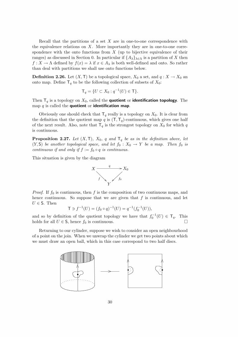
Returning to our cylinder, suppose we wish to consider an open neighbourhoodof a point on the join. When we unwrap the cylinder we get two points about whichwe must draw an open ball, which in this case correspond to two half discs.

� � � � � � � � � � � �� � � � � � � � � � � �

� � � � � � � � � � � �� � � � � � � � � � � �

30

The other thing we had to clarify was in what sense we can identify topologicalspaces. This is a key issue in the whole theory.

Definition 2.28. Let X and Y be topological spaces. A map f : X → Y is ahomeomorphism if f is a bijection such that both f and f−1 are continuous. Thespaces X and Y are said to be homeomorphic or topologically equivalent if sucha map f exists.

Homeomorphisms play the role in topology that bijections do in set theory orisomorphisms do in group or ring theory. In the topological context we are dealingwith sets where we have an extra structure, namely a notion of continuity, and sowe want to reflect that in our choice of maps.

Example 2.29.

(i) Any two bounded open intervals in R are homeomorphic: the map f :(a, b) → (c, d) defined through a combination of scaling and translation byf(x) = c+(d−c)(x−a)/(b−a) is a homeomorphism. There are many othersbetween these spaces.

(ii) We do not have to restrict ourselves to bounded intervals: (−1, 1) and Rare homeomorphic. For example consider the map f : (−1, 1) → R wheref(x) = x/(1− |x|), or the map g : (−1, 1) → R where g(x) = tan πx

2 .

(iii) A doughnut and a teacup are homeomorphic — they are both solid 3D shapesthat have only one hole in them. Neither are homeomorphic to the spherein R3, which has no holes.

(iv) The letter ‘L’ is homeomorphic to the letter ‘V’ — one is got from the otherby bending the arms closer together or further apart. However, neither arehomeomorphic to ‘T’. This follows since if X and Y are homeomorphic, viaa map f : X → Y , then so are A and f(A) for any subset A of X. So nownote that if we remove the junction point of ‘T’ then we get three separateparts, but if we remove any point from ‘L’ we get at most two parts.

It is straightforward to show that homeomorphism defines an equivalence re-lation on the set of topological spaces: if X and Y are homeomorphic, and ifY and Z are homeomorphic, then so are X and Z — just compose the relevanthomeomorphisms. Thus R is homeomorphic to (a, b) for any choice of a < b fromR.

A given property that a space may or may not possess is called a topologicalproperty if it is preserved by homeomorphisms. For instance, if X and Y arehomeomorphic and Y is Hausdorff, then it follows that X must also be a Hausdorffspace. This is actually a consequence of the following weaker result:

Proposition 2.30. Let f : X → Y be a continuous injective map between topo-logical spaces, and suppose that Y is Hausdorff. Then X is also Hausdorff.

Proof. Let x1, x2 ∈ X be distinct points. Since f is injective we have that f(x1) 6=f(x2), and since Y is Hausdorff we know that there are some open sets V1, V2 ⊂ Ysuch that f(xi) ∈ Vi, but V1 ∩ V2 = ∅. But f is also continuous, hence f−1(V1)

31

and f−1(V2) are open subsets of X. Moreover we have xi ∈ f−1(Vi) and f−1(V1)∩f−1(V2) = ∅. Thus X is Hausdorff as required.

As a final word on homeomorphisms, consider what happens when we cut cylin-ders and Mobius strips in half. Cutting a cylinder in half produces two cylinderswhich is clear from our usual picture of them:

� � � � � � � � � � � �� � � � � � � � � � � �� � � � � � � � � � � �� � � � � � � � � � � �

� � � � � � � � � � � �� � � � � � � � � � � �� � � � � � � � � � � �� � � � � � � � � � � �

� � � � � � � � � � � �� � � � � � � � � � � �� � � � � � � � � � � �� � � � � � � � � � � �

�� �����

This can also be shown by considering quotient topologies in the appropriate way:

two

cylinders

Here the change in arrows show which points are still being identified after thecut. However, if we apply the same reasoning to the Mobius band we find thefollowing:

one cylinder

Thus it follows that if we cut the Mobius band in half we only get one piece!Moreover that piece appears to be a cylinder. If you do this in practice you get

32

a cylinder with a double twist, which is a homeomorphic to the usual cylinder.However no amount of deformation in R3 will allow you to move from one surfaceto the other — the definition of homeomorphism applies to the surface/space itself,and not to any ambient space we may viewing it in.

Exercises

1. List all possible topologies on {a, b, c}. Consequently find a two topologies T1

and T2 on a set that are not comparable. That is, we have neither T1 ⊂ T2 norT2 ⊂ T1.

2. Give an example of subsets A and B of R for which A ∩ B, A ∩ B, A ∩ B andA ∩B are all different.

3. Let X be a topological space and A ⊂ X a subset. The boundary of A is definedto be b(A) = A ∩X \A. Calculate b(A) when A = (0, 1] and

(i) X = R, with the usual topology (ii) X = C, with the usual topology(iii) X = R, with the discrete topology (iv) X = C, with the indiscrete topology

4. Let {Tλ}λ∈Λ be a family of topologies on a set X. Show that⋂

λ∈Λ Tλ is a topologyon X, but that

⋃λ∈Λ Tλ need not be.

5. Given a topological space (Y, S) and a map f : X → Y , show that the collectionTf = {f−1(U) : U ∈ S} is a topology on X. Moreover, show that f is continu-ous with respect to this topology, and that Tf is the weakest topology with thisproperty.Describe this topology when we take X = Y = R, S to be the usual topology, andtake f to be (i) a constant function, (ii) the function that maps (−∞, 0] to 0 and(0,∞) to 1, and (iii) f(x) = x.

6. Prove that any map f : X → Y is continuous if either X is equipped with thediscrete topology or Y is equipped with the indiscrete topology.

7. Show that f : X → Y is continuous if and only if it is continuous as a map ontothe subspace f(X).

8. Let (X, T) be a topological space and let U be an open subset of X. Show that ifV is a subset of U that is open in the subspace topology TU , then V is open as asubset of X. Show that this can fail if we do not assume that U is open.

9. Let X1 be a topological space, and X2 a subset of X1 equipped with the subspacetopology. Let A be a subset of X2, and denote by Ai the closure of A in Xi, fori = 1, 2. Prove that (i) A2 = X2 ∩A1 (ii) if X2 is closed in X1 then A1 = A2.

10. Let X1, X2, Y1 and Y2 be topological spaces, and let f1 : X1 → Y1 and f2 : X2 → Y2

be maps. Define a map f : X1 ×X2 → Y1 × Y2 by

f((x1, x2)

)=

(f1(x1), f2(x2)

).

Show that f is continuous if and only if f1 and f2 are continuous, where X1 ×X2

and Y1 × Y2 are given their respective product topologies.

33

11. (a) Let X1 and X2 be topological spaces, and let W be an open subset of X1×X2.Show that pi(W ) is an open subset of Xi for i = 1, 2, where pi is the projectionmap X1 ×X2 → Xi.

(b) Give an example of a closed subset W ⊂ R×R such that p1(W ) is not closedin R.

12. Let X and Y be topological spaces and suppose that E ⊂ X and F ⊂ Y are closed.Show that E × F is closed in the topological product X × Y .

13. Let X = [−1, 1] equipped with the usual topology.

(a) Let f : X → [0, 1] be the function f(x) = |x|. Show that quotient topologyinduced on [0, 1] by f coincides with the usual topology.

(b) Find a surjection g : X → [0, 1] for which the quotient topology induced byg is not Hausdorff.

14. Prove that homeomorphism defines an equivalence relation on the class of alltopological spaces.

15. Show that if f : X → Y is a homeomorphism and A ⊂ X, then the restrictionsf |A : A → f(A) and f |X\A : X \A → Y \ f(A) are both homeomorphisms.

16. Let X1 and X2 be topological spaces, and pick a2 ∈ X2. Show that X1 is home-omorphic to the subspace X1 × {a2} of X1 × X2 respectively. Show that X1 ishomeomorphic to the subset {(x, x) : x ∈ X1} of X1 ×X1.

17. Let X be an infinite set, and let T be the Zariski topology, that is,

T = {∅} ∪ {U ⊂ X : X \ U is finite}.

Show that T is indeed a topology, but that it is not Hausdorff.

18. Prove the following:

(i) Any subspace of a Hausdorff space is Hausdorff.

(ii) The product of two Hausdorff spaces is Hausdorff.

(iii) If f : X → Y is continuous and injective, and Y Hausdorff, then so is X.

(iv) Being Hausdorff is a topological property, that is, it is preserved by home-omorphisms.

19. Show that in a Hausdorff space X, the set {x} is

(i) closed, and

(ii) the intersection of all open sets containing x.

20. Let f, g : X → Y be continuous maps between topological spaces, with Y Haus-dorff. Show that W = {x ∈ X : f(x) = g(x)} is closed in X. Deduce that iff : X → X is a continuous map and X is Hausdorff then the fixed point set{x ∈ X : f(x) = x} is closed.

21. A T1-space is a topological space (X, T) that satisfies the following: for any pair

34

of distinct points x, y ∈ X there are Ux, Uy ∈ T such that

x ∈ Ux, y ∈ Uy, but x /∈ Uy, y /∈ Ux.

Show that every Hausdorff space is a T1-space, but that there are T1-spaces thatare not Hausdorff.

35

3 Compactness

Compactness for topological spaces; the Heine-Borel Theorem

Several results in analysis concerning real-valued functions are trivial if the func-tion f is defined on a set X that is finite. For example, if we have X = {x1, . . . , xn}then f(X) ⊂ R is bounded and achieves its bounds, namely

f(xi1) = mini

f(xi) ≤ f(x) ≤ maxi

f(xi) = f(xi2)

for some 1 ≤ i1, i2 ≤ n. This result remains true if we replace X by a closed andbounded subinterval of R, and we stipulate that f be continuous. That is, we aredealing with a continuous function f : [a, b] → R for some a < b. This is oftengiven as part of the Intermediate Value Theorem. The particular property of [a, b]that makes this result true is the subject of this chapter.

Definition 3.1. Let X be a set and Y a subset of X. A cover for Y is anycollection U of subsets of X such that Y ⊂

⋃U∈U U . A subcover of the given

cover U is any subcollection V of U such that V is again a cover for Y . That is, ifU ∈ V then U ∈ U , and Y ⊂

⋃U∈V U .

A cover U is finite if there are only finitely many sets in U . If X is a topologicalspace then U is an open cover if each set in U is an open set.

Example 3.2. The singleton sets{{x}

}x∈R form a cover of R. Even though each

subset {x} is finite, there are infinitely many sets in the cover, so the cover is infi-nite. On the other hand {(−∞, 1), (−1, 1), (−1,∞)} is a cover of R comprising onlythree subsets, and hence is a finite cover. The subcollection {(−∞, 1), (−1,∞)} isa subcover, but the cover {(−∞, 1), (0,∞)} is not a subcover since (0,∞) is notone of the original subsets.

Unsurprisingly, since we are dealing with topological spaces, it will be opencovers that are of interest in this course.

Definition 3.3. A topological space X is compact if every open cover of X hasa finite subcover.

Note what this definition says: if we have any family U of open sets such thatevery element x ∈ X appears in at least one U ∈ U , then we actually only need afinite number of sets to capture all of the points. This is not the same as sayingthat there is at least one finite open cover of the space — this is always true sincewe can take U = {X}.

Example 3.4.

(a) Any topological space with a finite number of points is compact — givenany open cover just pick out one set for each point in the space to producea finite subcover.

(b) A discrete topological space X is compact if and only if it is finite. To showthis, note that if X is infinite then U =

{{x} : x ∈ X

}is an open cover of

X containing infinitely many sets, and if we leave any of them out then thecorresponding points will not lie in the union of the remaining sets.

36

(c) The subset (0, 1) of R is not compact: consider the family of open subsetsU = {( 1

n , 1) : n ≥ 2}. It is clear that⋃

n≥2(1n , 1) = (0, 1), so this is an

open cover. Any finite subfamily is of the form {( 1n1

, 1), . . . , ( 1nk

, 1)} forsome n1, n2, . . . , nk ∈ N, and so their union is ( 1

N , 1) $ (0, 1) where N =max{n1, . . . , nk}. Similarly, (0, 1] is not compact.

As ever there is an equivalent definition of compactness in terms of closedsets rather than open sets, and it is obtained from the above definition by takingcomplements. This process, applied to a cover, will not yield another cover. Hencewe need the following:

Definition 3.5. A family {Aλ}λ∈Λ of nonempty subsets of a set X has the finiteintersection property (FIP) if

⋂γ∈Γ Aγ 6= ∅ for every finite set Γ ⊂ Λ.

Proposition 3.6. Let X be a topological space. Then X is compact if and only if⋂λ∈Λ Fλ 6= ∅ for every family {Fλ}λ∈Λ of closed sets that has the FIP.

Proof. Suppose X is compact and {Fλ}λ∈Λ is a family of closed sets such that⋂λ∈Λ Fλ = ∅. Taking complements and using De Morgan’s Laws gives

⋃λ∈Λ F c

λ =X, and so {F c

λ}λ∈Λ is an open cover of X. Hence there is a finite subset Γ ⊂ Λsuch that

⋃γ∈Γ F c

γ = X, and taking complements once more gives⋂

γ∈Γ Fγ = ∅.Thus {Fλ}λ∈Λ does not have the FIP. Thus any family of closed sets having theFIP must have nonempty intersection.

Suppose the converse is true, that is, X is a topological space in which everyfamily of closed sets with the FIP has nonempty intersection. Let {Uλ}λ∈Λ be anopen cover of X, then ⋃

λ∈Λ Uλ = X ⇒⋂

λ∈Λ U cλ = ∅.

Thus {U cλ}λ∈Λ cannot have the FIP, hence there is a finite set Γ ⊂ Λ such that⋂

γ∈Γ U cγ = ∅. This in turn implies that

⋃γ∈Γ Uγ = X, and so we have a finite

subcover.

It is possible to consider compactness for subspaces of topological spaces, al-though we must take a little care to ensure that our definitions do not lead toconfusion.

Definition 3.7. Let (X, T) be a topological space and Y a nonempty subset ofX. Then Y is compact as a subspace if for any cover for Y taken from T, there isa finite subcover.

Note that in the above we are choosing the sets that make up the cover fromT, that is they are open subsets of the larger space X rather than open sets of Y .But in fact it turns out that Y is compact as a subspace of X if and only if it iscompact with respect to the subspace topology TY induced on Y by the topologyon X. To see this, suppose that Y is compact according to Definition 3.7 and thatU is any collection from TY that covers Y . Now each element of U is of the formU ∩ Y for some U ∈ T, and if we select a U ∈ T in this way for each set in thecover U , then we obtain a subcollection V of T that covers Y . Compactness of

37

Y in the sense of Definition 3.7 ensures that there is a finite subcover of V, say{U1, . . . , Un}, and then {U1 ∩Y, . . . , Un ∩Y } is a finite subcover of U . The reverseimplication is given by a very similar argument.

The above discussion thus frees us from having to be too pedantic about spec-ifying what we mean when we say a subspace is compact.

Perhaps the most important example of a compact space is the following:

Theorem 3.8 (Heine-Borel). Any closed bounded interval [a, b] in R is compact.

Proof. Note that we may assume that a < b otherwise our set contains only onepoint, and thus is clearly compact. So let U be any collection of open sets of Rthat covers the interval [a, b], and set

G = {x ∈ [a, b] : [a, x] can be covered by a finite subcover of U}.

The elements of G are to be thought of as the ‘good’ points, and we are aiming toshow that b ∈ G.

Now a ∈ G, since there is some U ∈ U such that a ∈ U , and so {U} is afinite subcover of U that covers [a, a] = {a}. Thus G 6= ∅ and G ⊂ [a, b], so if wedefine g = supG then g exists and also g ∈ [a, b]. Hence there is some U0 ∈ Usuch that g ∈ U0, and since U0 is open in R there must be some δ > 0 such that(g − δ, g + δ) ⊂ U0. However, by definition of g, there is some c ∈ G satisfyingg − δ < c ≤ g, and thus there is a finite subfamily {U1, . . . , Un} of U that covers[a, c]. Hence {U0, U1, . . . , Un} covers the subset [a, g + δ) of R, and we see that ifg < b then we would have contradicted the definition of g, since the points in thenonempty set (g, g + δ)∩ [a, b] would also lie in G. Thus g = b, and the set [a, b] iscovered by the finite subfamily {U0, U1, . . . , Un}. That is, b ∈ G as required.

The importance of the compactness of [a, b] lies in the following basic propertiesof compactness. In particular we will shortly be able to characterise all compactsubsets of Rn.

Proposition 3.9. Any closed subspace of a compact space is compact.

Proof. Let (X, T) be a compact space and F ⊂ X a nonempty subset that isclosed. Let U ⊂ T be an open cover of F consisting of open subsets of X. ThusF ⊂

⋃U∈U U , and so X = F c ∪ F = F c ∪

⋃U∈U U . But F c = X \ F is open

in X, hence {F c} ∪ U is an open cover of X. So we can choose a finite subcover{U1, . . . , Un, F c} of the cover for X, and it follows that the family {U1, . . . , Un}covers F as required.

Definition 3.10. A subset Y of a metric space (X, d) is bounded if there is someconstant K > 0 such that d(x, y) ≤ K for all x, y ∈ Y .

An alternative definition would say that there is some preferred point a ∈ Xand constant K ′ ≥ 0 such that d(a, x) ≤ K ′ for all x ∈ Y . That these definitionsactually single out the same class of subsets of X is an easy consequence of thetriangle inequality for metric spaces.

Definition 3.11. Let Y be a bounded subset of a metric space X. The diameterof Y , denoted diam Y , is sup{d(x, y) : x, y ∈ Y }.

38

It follows from the previous two results that any closed and bounded subsetA ⊂ R is compact. Boundedness of A implies that A ⊂ [−R,R] for some R > 0,which is compact by Theorem 3.8, and so A is a closed subset of a compact space,hence compact by Proposition 3.9. In fact the converse is true, which follows fromthe next two results which will be proved in far more generality than just dealingwith subsets of R.

Proposition 3.12. Let X be a compact metric space. Then X is bounded.

Proof. Pick any point x ∈ X. Then the collection of open balls {B(x, n)}n≥1 is afamily of open subsets of X that are nested, in the sense that

B(x, 1) ⊂ B(x, 2) ⊂ · · · ⊂ B(x, n) ⊂ B(x, n + 1) ⊂ · · ·

Moreover for any y ∈ X we have y ∈ B(x, n) for all n > d(x, y), and so⋃

n≥1 B(x, n) =X. But X is compact, so there must be a finite subcover, from which it followsthat X ⊂ B(x,N) for some N ≥ 1. Hence X is bounded, with diameter no greaterthan 2N .

Proposition 3.13. Any compact subset of a Hausdorff space is closed.

Proof. Let C be a compact subspace of a Hausdorff space X, and pick x ∈ Cc whichwe keep fixed for now. For each y ∈ C we can find open sets U(x, y) and V (x, y)such that x ∈ U(x, y), y ∈ V (x, y) and U(x, y)∩V (x, y) = ∅, since X is Hausdorff.Thus {V (x, y) : y ∈ C} is an open cover of C, and so there must be an finitesubcover, {V (x1, y1), . . . , V (xn, yn)} say. Let U(x) = U(x1, y1) ∩ · · · ∩ U(xn, yn),then U(x) is open and x ∈ U(x). Moreover U(x) has empty intersection with eachV (xi, yi) and so U(x) ∩

⋃ni=1 V (xi, yi) = ∅, hence U(x) ∩ C = ∅. Now varying our

point x, it follows that Cc =⋃

x∈Cc U(x), hence is open, and so C is closed.

Before we deal with products of compact spaces we shall take a brief diversionand consider their images under continuous maps.

Proposition 3.14. Let X be a compact space, Y a topological space, and f : X →Y and continuous map. Then f(X) is a compact subset of Y .

Proof. Let U be an open cover of f(X), that is U is a collection {Uλ}λ∈Λ of opensubsets of Y such that f(X) ⊂

⋃λ∈Λ Uλ. Now, by continuity of f , {f−1(Uλ)}λ∈Λ

is a family of open subsets of X, and moreover

f(X) ⊂⋃

λ∈Λ Uλ ⇒ X ⊂⋃

λ∈Λ f−1(Uλ) (⊂ X).

Thus {f−1(Uλ)}λ∈Λ is an open cover of the compact space X. Hence there is afinite subcover, so for some finite set Γ ⊂ Λ

X =⋃

γ∈Γ f−1(Uγ) ⇒ f(X) =⋃

γ∈Γ f(f−1(Uγ)

)⊂

⋃γ∈Γ Uγ ,

and so {Uγ}γ∈Γ is a finite subcover of f(X).

This very general result tells us that compactness is a topological property,and leads immediately to easy corollaries that deal with familiar situations.

39

Corollary 3.15. Let X and Y be homeomorphic spaces. Then X is compact ifand only if Y is compact.

Proof. Let f : X → Y be a homeomorphism, and suppose that X is compact,then Y = f(X) is compact. If, on the other hand, we are given that Y is compact,then X = f−1(Y ) is compact (where here we are, for once, really dealing with aninverse function f−1!).

Corollary 3.16. Let X be a compact space, Y a metric space and f : X → Y acontinuous map. Then f(X) is closed and bounded.

If Y = R then there are points x1, x2 ∈ X such that f(x1) = inf f(X) andf(x2) = sup f(X). That is, f attains its bounds.

Proof. By Proposition 3.14 we know that f(X) is compact, and hence it is closedand bounded by Propositions 3.13 and 3.12. If Y = R, then the numbers inf f(X)and sup f(X) exist. Moreover, for any bounded set A ⊂ R, either inf A ∈ A or inf Ais a limit of points from A. Since f(X) is closed we must have inf f(X) ∈ f(X),hence the required point x1 must exist, and similarly for x2.

Thus this corollary, together with the Heine-Borel Theorem, tells us a lotabout the behaviour of continuous maps f : [a, b] → R. More importantly theabove results apply in far more general situations. To get to such situations it isuseful to have the following:

Proposition 3.17. Let X1 and X2 be topological spaces and set X = X1 × X2.Then X is compact if and only if X1 and X2 are compact.

Proof. We do the easy half of this proposition first — suppose that X is compact.Then Xi = pi(X) where pi is the coordinate projection. That is, Xi is the imageof a compact space under a continuous map, and hence is compact.

So now suppose instead that the components are both compact and letW be anopen cover of X. We call any subset A ⊂ X1 good if there is a finite subcollectionof W that covers A ×X2. We are aiming to show that X1 is a good set, and dothis in three steps.

Step 1: Let A1, . . . , Am ⊂ X1 be good subsets, then A = A1 ∪ · · · ∪ Am is good.For A×X2 =

⋃mi=1(Ai×X2), and so if Wi is a finite subcollection of W that covers

Ai ×X2, then W1 ∪ · · · ∪Wn is a finite subcollection of W that covers A×X2.

Step 2: Each point x ∈ X1 is locally good in the sense that there is an neighbour-hood Ux of x that is good.

To show this, pick x ∈ X. Then for each y ∈ X2 there is some W (y) ∈ Wsuch that (x, y) ∈ W (y). But, by definition of the product topology, we can findU(y) and V (y), open in X1 and X2 respectively, such that (x, y) ∈ U(y)× V (y) ⊂W (y). Now {V (y) : y ∈ Y } is an open cover of the compact space X2, sincey ∈ V (y) for each y, hence there is a finite subcover, {V (y1), . . . , V (yn)} say. SetUx = U(y1) ∩ · · · ∩ U(y1), then Ux is open in X and contains x. Moreover

Ux ×X2 = Ux ×⋃n

i=1 V (yi) =⋃n

i=1(Ux × V (yi))⊂

⋃ni=1(U(yi)× V (yi)) ⊂

⋃ni=1 W (yi),

40

and so Ux is a good set, as required.

Step 3: X1 is a good set. This final step is achieved by noting that for eachx ∈ X1 we have found an open set Ux that is both good and contains x. Thusin particular {Ux : x ∈ X} is an open cover of X1. But then compactness of X1

says that there is a finite subcover, {Ux1 , . . . , Uxk} say. So X1 =

⋃ki=1 Uxi , a finite

union of good sets, and thus X1 is good by step 1, which is what we set out toshow.

The above now clearly extends to any finite product of compact spaces by aninduction argument. What is perhaps surprising is that this is also true for anarbitrary product of compact spaces. This general form is Tychonoff’s Theorem,and is the basis for many important results in analysis. An account of this is givenin Simmons’ book. It turns out that Tychonoff only proved the result in a specialcase from which he then produced the Stone-Cech compactification. MeanwhileCech proved the general case of Tychonoff’s Theorem. . .

Putting a number of the above results together we finally arrive at a characteri-sation of the compact subsets of Rn, and hence also of Cm (since C is homeomorphicto R2, hence Cm is homeomorphic to R2m).

Theorem 3.18 (Heine-Borel). A subset of Rn is compact if and only if it isclosed and bounded.

Proof. Let C be a compact subset of Rn. Then it is closed by Proposition 3.13and bounded by Proposition 3.12.

Suppose instead that C is a closed and bounded subset of Rn. Then C ⊂[−R,R]n for some suitably large R. Now [−R,R] ⊂ R is compact by Theorem 3.8,and hence so is [−R,R]n by Proposition 3.17. But if C is a closed subset of Rn,then it is a closed subset of [−R,R]n, and hence compact by Proposition 3.9.

One way to think of compactness is that a topology that is compact cannothave ‘too many’ open sets, in the sense that we cannot build up any open coverthat is badly behaved. On the other hand a topology that is Hausdorff has aplentiful supply of open sets since we can use them to separate any two distinctpoints. This two conditions thus work against each other — one can show that ifX is a set and T and S are topologies on X that make X Hausdorff and compactrespectively, and if T ⊂ S, then we must have T = S.

Compactness for metric spaces: sequential compactness

When dealing with metric spaces it often makes sense to use sequences, and indeedwhen it comes to studying compactness there is no change to this rule of thumb. Inthis section we show that there is another equivalent formulation of compactnessthat is given in terms of sequences and their possible subsequences.

Definition 3.19. A subset C of a metric space X is sequentially compact initself (respectively in X) if every sequence in C has a subsequence that convergesto a point of C (resp. to a point of X).

41

It is clear that if C is sequentially compact in itself then it will be sequentiallycompact in X. On the other hand by Proposition 1.23, if C is sequentially compactin X then it is sequentially compact in itself if and only if it is closed.

The main result in this direction allows us to pass freely from sequential com-pactness, which is a natural concept for metric spaces, to the general idea ofcompactness as explained above.

Theorem 3.20. Let X be a metric space. Then X is compact if and only if it issequentially compact.

Proof. Suppose first that X is compact, and let (xn)n≥1 be any sequence in X.For each m ≥ 0 set Am = {xn : n > m} and Fm = Am. Since Am ⊃ Am+1, wehave Fm ⊃ Fm+1. Moreover, each Fm is closed and nonempty by construction,and so it follows that {Fm}m≥0 has the FIP. Hence, by Proposition 3.6, we musthave

⋂∞m=0 Fm 6= ∅.

So now let x ∈⋂∞

m=0 Fm. Then x ∈ F0 = A0, and so we must have B(x, 12) ∩

A0 6= ∅. So we can choose some n1 ≥ 1 such that d(xn1 , x) < 12 . Since x ∈

Fn1 = An1 , there is some n2 > n1 such that d(xn2 , x) < 14 . Repeating this, we find

n1 < n2 < n3 < · · · such that d(xnr , x) < 2−r, and hence xnr → x. Thus X issequentially compact.

Suppose instead that X is a sequentially compact metric space, and let U beany open cover of X. Our first step is to show that

∃ε > 0 s.t. ∀x ∈ X ∃Ux ∈ U s.t. B(x, ε) ⊂ Ux. (†)

So suppose that (†) does not hold, then

∀ε > 0 ∃x ∈ X s.t. ∀U ∈ U , B(x, ε) 6⊂ U.

For each n ≥ 1 we can put ε = 2−n in the above and find some xn ∈ X suchthat B(xn, 2−n) 6⊂ U for all U ∈ U . Since X is sequentially compact, there is asubsequence (xnr)r≥0 of this sequence that converges to some x ∈ X, and sinceU is a cover of X, there is some U ∈ U such that x ∈ U . But U is open so, forsome m ≥ 1, B(x, 2−m) ⊂ U and, given this m, we can find some R ≥ 1 such thatd(xnr , x) < 2−m−1 for all r ≥ R.

So now choose any r ≥ R for which nr > m, then

B(xnr , 2−nr) ⊂ B(xnr , 2

−m−1) ⊂ B(x, 2−m) ⊂ U,

using the triangle inequality for the second inclusion, and hence contradicting thechoice of xnr above. Hence (†) must hold after all.

Now suppose that U has no finite subcover. Pick any point x1 ∈ X, andconsider the corresponding Ux1 ∈ U for which B(x1, ε) ⊂ Ux1 , whose existence isguaranteed by (†). Since there is no finite subcover of U , Ux1 6= X, and so wecan choose x2 /∈ Ux1 . Then d(x1, x2) ≥ ε, and if we consider the correspondingUx2 ∈ U , then Ux1 ∪Ux2 6= X, hence B(x1, ε)∪B(x2, ε) 6= X, and so we can choosex3 ∈ X such that d(x1, x3) ≥ ε and d(x2, x3) ≥ ε. Iterating this procedure we

42

obtain a sequence (xn)n≥1 such that d(xm, xn) ≥ ε for all m < n. This sequencecannot have a convergent subsequence, for if xnr → x then we would have

ε ≤ d(xnr , xnr+1) ≤ d(xnr , x) + d(x, xnr+1) → 0

as r → ∞. Hence the existence of this sequence contradicts our assumption ofsequential compactness, and we’re done.

This alternative characterisation of compactness for metric spaces leads to analternative proof of one half of the Heine-Borel Theorem, namely that any closedand bounded subset of Rm is compact. It is based on the Bolzano-WeierstrassTheorem:

Theorem 3.21 (Bolzano-Weierstrass). Every bounded sequence of real num-bers has a convergent subsequence.

So let A ⊂ Rm be a closed and bounded subset, let (x(n))n≥1 be any sequencein A, where x(n) = (x(n)

1 , x(n)2 , . . . , x

(n)m ) for x

(n)i ∈ R. So we have

x(1) = (x(1)1 , x

(1)2 , x

(1)3 , . . .)

x(2) = (x(2)1 , x

(2)2 , x

(2)3 , . . .)

x(3) = (x(3)1 , x

(3)2 , x

(3)3 , . . .) etc.

The sequence of first coordinates (x(n)1 )n≥1 is a bounded sequence in R, and so has

a convergent subsequence. So for some infinite subset σ1 ⊂ N the (sub)sequence(x(n)

1 )n∈σ1 is convergent. But then (x(n)2 )n∈σ1 is a bounded sequence in R, hence

there is an infinite subset σ2 ⊂ σ1 such that (x(n)2 )n∈σ2 is convergent, and note also

that the subsequence (x(n)1 )n∈σ2 of our first subsequence will still be convergent.

Continuing this way we will eventually produce an infinite subset σm ⊂ N for whicheach sequence (x(n)

i )n∈σm of real numbers is convergent, and hence the sequence(x(n))n∈σm of points is also convergent to some x ∈ Rm. Finally, since A is closed,it contains the limits of all sequences taken from A, so that x ∈ A. Thus A issequentially compact, hence compact.

Exercises

1. Show that every finite topological space is compact. Show that a discrete topo-logical space is compact if and only if it is finite.

2. Let Y be a subspace of a topological space X and let Z be a nonempty subset ofY . Show that Z is compact as a subspace of Y if and only if it is compact as asubspace of X.

3. Let Y and Z be compact subspaces of a topological space X. Show that Y ∪ Z isa compact subspace of X.Let {Yλ}λ∈Λ be a family of compact and closed subsets of X such that

⋂λ Yλ 6= ∅.

Show that this intersection is compact. [Hint: use question 2.]

43

4. Let T1 and T2 be topologies on a set X, with T1 ⊂ T2. Show that if X is compactwith respect to T2 then it is also compact with respect to T1.

5. Which of the following subsets of R and R2 are compact?

(i) [0, 1) (ii) [0,∞) (iii) Q ∩ [0, 1]

(iv) {(x, y) ∈ R2 : x2 + y2 = 1} (v) {(x, y) ∈ R2 : x2 + y2 ≤ 1}(vi) {(x, y) ∈ R2 : x2 + y2 < 1} (vii) {(x, y) ∈ R2 : x ≥ 1, 0 ≤ y ≤ 1

x}

6. Let (Fn)n≥1 be a sequence of nonempty closed subsets of a compact topologicalspace X such that Fn ⊃ Fn+1 for all n. Show that

⋂n≥1 Fn 6= ∅.

7. Let C1 and C2 be compact subspaces of a Hausdorff space. Show that C1 ∩ C2 iscompact.

8. Suppose that X is a compact topological space, Y is a Hausdorff topological spaceand f : X → Y a continuous bijection. Show that X and Y are homeomorphic.[Hint: consider the closed subsets viewpoint of continuity.]

9. Show that R equipped with the Zariski topology is compact.

10. Let X be a compact metric space and suppose that f : X → X a continuousmap for which f(x) 6= x for all x ∈ X. Show that there is some ε > 0 such thatd(f(x), x) ≥ ε for all x ∈ X.[Hint: consider the map g : X → R given by g(x) = d(f(x), x).]

11. Let X be a compact metric space and f : X → X a continuous map. Show thatthere is a nonempty closed set F ⊂ X such that f(F ) = F .[Hint: consider the sequence F1 = f(X), Fn+1 = f(Fn), and question 6.]

12. Show that a compact metric space is separable.

13. Let (X, T) be a topological space. Set X ′ = X ∪ {∞}, where ∞ is any object notin X, and

T′ = T ∪ {V ∪ {∞} : V ⊂ X, X \ V is compact and closed in X}.

Prove that (X ′,T′) is a compact space containing X as a subspace.[This is the one-point or Alexandroff compactification — see Simmons p.163]

44

4 Connectedness

Equivalent definitions; subintervals of R

This section of our course deals with the idea of how many ‘chunks’ or ‘pieces’ agiven topological space splits up into. Intuitively a connected space is one that doesnot fall apart, for instance the subspace [0, 1] of R would be considered connected,but [0, 1] ∪ [2, 3] is not. However, what about more complicated spaces such asQ or the graph of the function y = sin 1

x? We shall discuss two different ways offormulating this idea more precisely.

Definition 4.1. A topological space X is connected if it cannot be written asX = U ∪ V where U and V are disjoint nonempty open subsets of X.

Every author has different terminology for the representation of a space X asU ∪ V in terms of disjoint open sets U and V . One route is to call the pair (U, V )a partition (into open sets), with the idea being that any set theoretic partitionof a topological space should be done using open sets, and hoping to thus avoidconfusion. Simmons is a little more inventive:

Definition 4.2. A space X is disconnected if it can be written as X = U ∪ Vfor disjoint nonempty sets U and V . If X is disconnected then any representationof this form is called a disconnection of X, noting that there may be many suchrepresentations. Indeed, the space X is called totally disconnected if for everypair of distinct points x, y ∈ X there is a disconnection (U, V ) such that x ∈ Uand y ∈ V .

Note. There are other definitions of totally disconnected in the literature, whichare similar in spirit to the one above but not necessarily equivalent.

There are several important things to spot arising from these definitions. Oneis that a one point space, X = {x}, is both connected and totally disconnected!Also note that if (U, V ) is a disconnection for a space X, then

X = U ∪ V and U ∩ V = ∅ ⇒ U = V c and V = U c,

and so the sets that make up the disconnection are both open and closed. It followsthat a topological space X is connected if and only if the only sets that are bothopen and closed are ∅ and X. Some authors used the word ‘clopen’ to describe aset that is both open and closed. Finally, note that any totally disconnected spaceis Hausdorff.

We now want to explore this new concept in the context of subspaces of R. Itwill turn out that the connected subspaces of R are precisely the intervals, and inshowing this we make use of the following easily proved lemma:

Lemma 4.3. A subset X ⊂ R is an interval if and only if whenever x, y, z ∈ Rare three points satisfying x < z < y and x, y ∈ X, we must have z ∈ X.

Theorem 4.4. A subspace X ⊂ R is connected if and only if it is an interval.

45

Proof. Suppose X is not an interval, then we can find x < z < y in R such thatx, y ∈ X, but z /∈ X. Now (−∞, z) and (z,∞) are open subsets of R, henceU = X ∩ (−∞, z) and V = X ∩ (z,∞) are open subsets of X such that x ∈ U andy ∈ V . But X = U ∪ V since z /∈ X, and U ∩ V = ∅ by construction. Thus (U, V )is a disconnection of X, and so X is not connected.

For the converse we first show that for any a < b there is no disconnection(U, V ) of [a, b] such that a ∈ U and b ∈ V . To see this, suppose that such apair (U, V ) of open sets does exist. Then U and V are also closed subsets of [a, b]and hence closed and bounded subsets of R. Moreover b ∈ V , so V 6= ∅. Settingc = inf V , then V ⊂ [a, b] implies that c ∈ [a, b], and V being closed implies thatc ∈ V . In particular c 6= a since a ∈ U . But c is a lower bound for V and a < c,hence c− 1

n ∈ U for all n ≥ (c−a)−1. Then c = limn(c− 1n) ∈ U , since U is closed,

giving U ∩ V 6= ∅, which contradicts the fact that (U, V ) is a disconnection.Now suppose that X is an interval that is disconnected. So X = U ′ ∪ V ′ for

nonempty disjoint open subsets U ′ and V ′ of X. Without loss of generality wecan pick a ∈ U ′ and b ∈ V ′ such that a < b, but then putting U = U ′ ∩ [a, b]and V = V ′ ∩ [a, b] gives a disconnection (U, V ) of [a, b] with a ∈ U and b ∈ V .So, by contradiction once again, X cannot be disconnected, hence every intervalis connected.

It follows from this characterisation that Q is not connected, since it is certainlynot an interval of R. In fact the rational numbers form a totally disconnectedsubspace of R: given any p, q ∈ Q with p < q we can find some irrational r suchthat p < r < q, and then

(Q ∩ (−∞, r), Q ∩ (r,∞)

)is a disconnection of Q that

separates p and q.An alternative to talking about disconnections is the idea that if a space falls

apart into more than one component then we should be able to define a continuousfunction on the space such that the values taken by the function on one componentbear no relation to those taken on the other component. This forms the basis foran equivalent definition of connectedness. Since a disconnection is only made upof two subsets, it is sufficient to consider functions that take only two values.

Proposition 4.5. A topological space X connected if and only if there is no con-tinuous map from X onto a discrete two point space.

Remark. Since all discrete two point spaces are homeomorphic to one another, itfollows that we can focus on the existence or nonexistence of continuous maps fromX onto {0, 1}.

Proof. Suppose that X is a topological space and that f : X → {0, 1} is acontinuous surjection. Set U = f−1({0}) and V = f−1({1}), then U ∪ V =f−1({0} ∪ {1}) = X and U ∩ V = f−1({0} ∩ {1}) = ∅. Moreover, since f is onto,neither U nor V can be empty, and, since f is continuous, both of these sets areopen. Hence we have a disconnection, and so X is not connected.

Conversely, suppose that X is not connected, so then there is a disconnection(U, V ) of X. Define a map f : X → {0, 1} by

f(x) =

{0 if x ∈ U,

1 if x ∈ V.

46

This is possible since U ∩ V = ∅, and f is onto since U 6= ∅ 6= V . Moreover, theopen subsets of {0, 1} are ∅, {0}, {1} and {0, 1}, and their preimages are ∅, U , Vand X respectively. Hence f is a continuous surjection X → {0, 1}.

An immediate corollary of the next result is that connectedness is a topologicalproperty.

Corollary 4.6. Let f : X → Y be a continuous map between topological spaces,with X connected. Then f(X) is a connected subspace of Y .

Proof. Suppose that f(X) is not connected, then there must be a continuoussurjection g : f(X) → {0, 1}. It follows that the composition g ◦ f : X → {0, 1} iscontinuous and onto, and hence X cannot be connected.

Combining this with the characterisation of connected sets of R (Theorem 4.4)gives the following:

Corollary 4.7. If X is a connected space and f : X → R is a continuous map,then f(X) is an interval.

The obvious application of this result (together with our work on compactness)to real analysis, is a proof by abstract means of the Intermediate Value Theorem:if f : [a, b] → R is a continuous map then f([a, b]) is a compact and connectedsubset of R, hence must be of the form [c, d] for some c < d in R.

As with all of the properties we have considered, we would like to know howconnectedness behaves when we pass to subspaces, build products etc. Indeed, wehave already seen examples of spaces that are not connected, but are subspaces ofconnected space (e.g. Q ⊂ R).

Proposition 4.8. Let X be a topological space, let {Aλ}λ∈Λ be a family of sub-spaces such that each Aλ is connected, and suppose that for some λ0 ∈ Λ we haveAλ ∩Aλ0 6= ∅ for all λ ∈ Λ. Then A =

⋃λ∈Λ Aλ is connected.

Proof. Let f : A → {0, 1} be a continuous map. We must show that f is not onto.Since f is continuous, the restriction f |Aλ

is continuous for each λ ∈ Λ, and somust be constant. That is, for some yλ ∈ {0, 1} we have f(x) = yλ for all x ∈ Aλ.But then for each λ we can choose xλ ∈ Aλ ∩Aλ0 , so yλ = f(xλ) = yλ0 , and hencef(x) = yλ0 for all x ∈ A. Thus A is connected.

Corollary 4.9. Let X1 and X2 be connected spaces. Then X = X1 × X2 isconnected if and only if X1 and X2 are connected.

Proof. First note that Xi is the image of X under the continuous projection mappi, and so each Xi must be connected if X is connected, by Proposition 4.6.

Suppose instead that X1 and X2 are connected. We shall apply Proposition 4.8with Λ = {0}∪X2. Pick x ∈ X1 and set A0 = {x}×X2. Then A0 is homeomorphicto X2 (exercise), and hence connected. Similarly, for each y ∈ X2 set Ay =X1 × {y}, then each Ay is homeomorphic to X1 and hence connected. Moreover,A0 ∩Ay = {(x, y)} 6= ∅, and

X =⋃

y∈X2Ay ⊂ A0 ∪

⋃y∈X2

Ay ⊂ X.

47

Path-connectedness

When considering whether or not a subset S of R2 or R3 is connected, our mentalpicture is probably to check if every pair of points in S can be joined by some sortof path that lies in S. This is the basis of a very important, but slightly different,method of approaching this topic.

Definition 4.10. Given two points a, b in a topological space X, a path from ato b is a continuous map f : [0, 1] → X such that f(0) = a and f(1) = b.

Definition 4.11. A topological space is path-connected if every two points inthe space can be connected by a path.

This definition turns out to be a specialisation of the one we have been usingup to now:

Proposition 4.12. Any path-connected space is connected.

Proof. Suppose that X is a path-connected space and let f : X → {0, 1} be acontinuous map. Let x, y ∈ X, then there a path from x to Y , i.e. a continuousmap g : [0, 1] → X with g(0) = x and g(1) = y. But then f ◦ g : [0, 1] → {0, 1} isa continuous map on the connected space [0, 1], and hence must be constant. Sonow we have

f(x) = f(g(0)

)= f

(g(1)

)= f(y),

thus f must be constant, and so X is connected.

It turns out that the converse is not true — an example of a connected spacethat is not path-connected is given on the exercise sheets. However for a largeclass of spaces the converse is true, as shown in Proposition 4.14 below. First,however, we need to consider the composition of paths.

Lemma 4.13. Let X be a topological space and suppose that x, y, z ∈ X are pointssuch that x and y can be connected by a path, and y and z can be connected by apath. Then x and z can be connected by a path.

Proof. By hypothesis there are continuous maps f : [0, 1] → X and g : [0, 1] → Xsuch that f(0) = x, f(1) = g(0) = y and g(1) = z. Defining h : [0, 1] → X by

h(t) =

{f(2t) if t ∈ [0, 1

2 ],g(2t− 1) if t ∈ [12 , 1]

gives a continuous map such that h(0) = x and h(1) = z.

Proposition 4.14. Any open connected subset U of Rn is path-connected.

Proof. Fix a point a ∈ X, and let H be the set of points that can be connected toa by a path in U . We must show that K = U \H is empty.

First we shall show that H is open in U (equivalently, open in Rn). So letx ∈ H, then for some ε > 0 we have B(x, ε) ⊂ U . Given any y ∈ B(x, ε) wecan connect it to x, the centre of this ball, by the radial path. Thus, there is a

48

path from a to x, and then a path from x to y, and these can be composed usingLemma 4.13 to give a path from a to y. Hence B(x, ε) ⊂ H, and so H is open inU (and Rn). A similar argument shows that K must also be open. But now bydefinition we have H ∪K = U , and H ∩K = ∅. Furthermore, U is connected, andH 6= ∅, hence K = ∅ as required.

Exercises

1. Let T1 and T2 be topologies on a set X satisfying T1 ⊂ T2. Is (X, T1) connectedif (X, T2) is connected? Is (X, T2) connected if (X, T1) is connected?

2. Let X be a connected space containing more than one point, and suppose that{x} is closed for each x ∈ X. Show that the number of points in X is infinite.

3. Prove that any continuous function f : [a, b] → [a, b] has a fixed point.[Hint: consider the function g : [a, b] → R given by g(x) = f(x)− x.]

4. (a) Prove that if X is a connected space and there is a continuous map f : X → Rthat is not constant, then X is uncountably infinite.

(b) Prove that if X is a connected metric space with more than one point, thenit has uncountably many points.

5. Prove that there is no continuous injective map f : R2 → R. Can the spaces R2

and R be homeomorphic? Is the line R homeomorphic to [−1, 1]?

6. Let f : [0, 1] → R be a continuous map such that f(0) = f(1). Let n ≥ 2.Show that there is some x ∈ [0, 1] such that f(x) = f(x + 1

n). [Hint: let g(x) =f(x)− f(x + 1

n) and show that g(0) + g( 1n) + · · ·+ g(n−1

n ) = 0.]

7. Prove that any discrete space is totally disconnected.

8. Give an example of connected subsets Cn ⊂ R2 such that Cn ⊃ Cn+1 for all n ≥ 1,but such that

⋂n≥1 Cn is not connected. Can you find an example for which all of

the Cn are closed?

9. Prove that there is no continuous map f : [0, 1] → R satisfying x ∈ Q ⇔ f(x) /∈ Q.

10. Consider the following subset of R2: A = {(x, y) ∈ R : x 6= 0, y = sin 1x}. Is A

connected or disconnected? Answer the same question for the subsets A∪{(0, 0)}and A ∪ ({0} × [−1, 1]).[Hint: first prove the following result. If B and C are subsets of a topologicalspace X with B connected and B ⊂ C ⊂ B, then C must also be connected. Toshow this note that any continuous map f : C → {0, 1} restricts to a continuousmap B → {0, 1}, which must be constant.]

49

5 Completeness and Uniformity

Uniform convergence and continuity

When dealing with a collection of functions defined on some given set X, we wouldlike some notion of whether or not two of these functions are close to each other,or whether a sequence from the collection converges. A natural method is to lookat the behaviour at each point x in the space, but this does not always guaranteerespectable outcomes.

Definition 5.1. Let X be a set and (fn) a sequence of functions from X into ametric space (Y, d). The sequence converges pointwise to a function f : X → Y iff(x) = limn fn(x) for each x ∈ X. Here we are using the definition of convergencein a metric space as introduced in the first section. So fn converges pointwise tof if

∀x ∈ X, ε > 0 ∃N ≥ 1 s.t. d(f(x), fn(x)

)< ε ∀n ≥ N.

Here the N depends on the choice of both x and ε.The sequence converges uniformly to the function f if

∀ε > 0 ∃N ≥ 1 s.t. d(f(x), fn(x)

)< ε ∀x ∈ X, n ≥ N.

That is, there is some N that does the job for all of the points x ∈ X simultane-ously.

It is possible in certain circumstances to reinterpret uniform convergence as theusual convergence with respect to a given metric. For instance let X = C[0, 1], thespace of continuous functions from [0, 1] to C, equipped with the following metric:

d∞(f, g) = supx∈[0,1]

|f(x)− g(x)|.

Now suppose that f ∈ X and (fn) is a sequence in X such that fn → f withrespect to d∞. This means that for any given ε > 0 we can find some N ≥ 1 suchthat d∞(f, fn) < ε for every n ≥ N . But if this is so then

n ≥ N ⇒ |f(t)− g(t)| ≤ supx∈[0,1]

|f(x)− g(x)| = d∞(f, g) < ε ∀t ∈ [0, 1]

That is, the functions fn converge uniformly to the function f . For this reason d∞is often known as the uniform metric.

Note that d∞ can be defined in the same way on the set B(X; R) of all boundedfunctions from any given set X into R, and again a sequence in B(X; R) convergesto some other function in B(X; R) uniformly if and only if it converges with respectto the uniform metric. Here we need to restrict ourselves to bounded functions inorder to make sense of d∞, but the concept of uniform convergence applies morewidely: if we consider the functions fn and f defined on R by

fn(x) = x2 + 1n , f(x) = x2

then fn converges to uniformly to f , since fn(x) − f(x) = 1n for all choices of

x ∈ R, but none of the functions involved are bounded.

50

Example 5.2. Consider the functions fn(x) = xn defined for x ∈ [0, 1]. Then wehave fn(x) → f(x) pointwise, where

f(x) =

{0 if x ∈ [0, 1),1 if x = 1.

Thus this sequence of continuous functions converges pointwise to a discontinuousfunction. It follows from the next result that fn does not converge uniformly to f .

Proposition 5.3. Let X and Y be metric spaces, and let (fn) be a sequence offunctions from X to Y each of which is continuous at x0 ∈ X. If fn convergesuniformly to a function f : X → Y , then f is continuous at x0.

Remark. Thus, if a family of continuous functions converges uniformly then thelimit must be a continuous function.

Proof. Fix ε > 0. Since fn → f uniformly there is some N ≥ 1 such that ifn ≥ N , then dY

(f(x), fn(x)

)< ε

3 for every x ∈ X. In particular this is true forn = N . But fN is continuous at the point x0, and so there is some δ > 0 suchthat dY

(fN (x), fN (x0)

)< ε

3 whenever x ∈ X satisfies dX(x, x0) < δ. So now ifdX(x, x0) < δ then

dY

(f(x), f(x0)

)≤ dY

(f(x), fN (x)

)+dY

(fN (x), fN (x0)

)+dY

(fN (x0), f(x0)

)<

ε

3× 3 = ε,

and thus f is continuous at x0 as required.

The above proposition is one that is frequently invoked whenever we need tochange the order in which limits are taken. In effect what we have proved is thatif fn → f uniformly, and all of the fn are continuous at x0 then

limx→x0

(lim

n→∞fn(x)

)= lim

n→∞

(lim

x→x0

fn(x)).

Example 5.4. As an example of a sequence of continuous functions that convergepointwise but not uniformly to a continuous function (indeed, a constant function)consider the following ‘moving bump’:

1

1

1

1

1

1

f1 f2 f3

1

2

1

3

51

We have that fn(x) → 0 for every x ∈ [0, 1], but fn( 12n) = 1 for each n. So given

any 0 < ε < 1 there can be no N ≥ 1 for which |fn(x)− 0| < ε for every x ∈ [0, 1]and n ≥ N .

A counterpart to uniform convergence is uniform continuity, and this now re-quires that our domain X be a metric space, rather than merely a set.

Definition 5.5. Let X and Y be metric spaces. A function f : X → Y isuniformly continuous if for each ε > 0 there is some δ > 0 such that

dX(x, x′) < δ ⇒ dY

(f(x), f(x′)

)< ε.

The distinction between continuity as discussed earlier and uniform continuityis that for the given ε we can find a δ such that whenever we pick any two pointsx and x′ that are within δ of each other, then their images are within ε of eachother. That is, the δ is independent of the points in question.

Example 5.6. The simplest example of a uniformly continuous map is constructedas follows: given a pair of metric spaces X and Y , pick a point y0 ∈ Y and definef : X → Y by setting f(x) = y0 for every x ∈ X. Then dY

(f(x), f(x′)

)= 0 for

every pair of points x, x′ ∈ X, and so given ε > 0 we may take δ to be any positivenumber.

Uniform continuity plays an important role in real and complex analysis, as it isa significant strengthening of the usual notion of continuity. The next result showsthat we encounter this happy situation more frequently than one may imagine onfirst seeing the definition.

Proposition 5.7. Let X and Y be metric spaces, with X compact. Then anycontinuous function from X to Y is uniformly continuous.

Proof. Let ε > 0. For each x ∈ X we can find some δx > 0 such that

dX(x, x′) < 2δx ⇒ dY

(f(x), f(x′)

)<

ε

2(∗)

and the resulting collection of open balls, {B(x, δx) : x ∈ X} (note the halving ofthe radii), is an open cover of X. Hence there is a finite subcover, {B(x1, δx1), . . . , B(xn, δxn)}say, since X is compact.

Set δ = min{δx1 , . . . , δxn}, and consider any pair of points x, x′ ∈ X suchthat dX(x, x′) < δ. Now x ∈ B(xi, δxi) for some 1 ≤ i ≤ n. So by (∗) we havedY

(f(x), f(xi)

)< ε

2 . Also,

dX(x′, xi) ≤ dX(x′, x) + dX(x, xi) < δ + δxi < 2δxi .

But then dY

(f(x′), f(xi)

)< ε

2 by (∗) again, and putting these two inequalitiestogether by means of the triangle inequality gives

dY

(f(x), f(x′)

)≤ dY

(f(x), f(xi)

)+ dY

(f(xi), f(x′)

)<

ε

2+

ε

2= ε

as required.

52

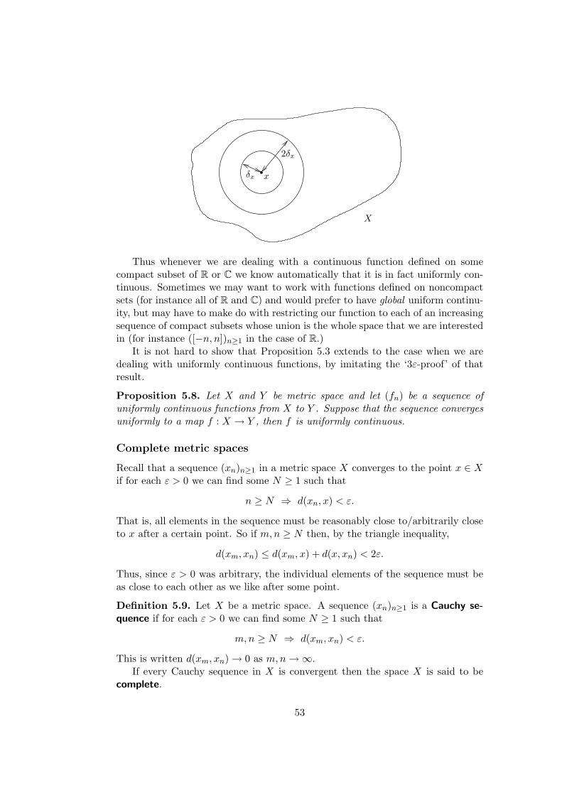
X

xδx

2δx

Thus whenever we are dealing with a continuous function defined on somecompact subset of R or C we know automatically that it is in fact uniformly con-tinuous. Sometimes we may want to work with functions defined on noncompactsets (for instance all of R and C) and would prefer to have global uniform continu-ity, but may have to make do with restricting our function to each of an increasingsequence of compact subsets whose union is the whole space that we are interestedin (for instance ([−n, n])n≥1 in the case of R.)

It is not hard to show that Proposition 5.3 extends to the case when we aredealing with uniformly continuous functions, by imitating the ‘3ε-proof’ of thatresult.

Proposition 5.8. Let X and Y be metric space and let (fn) be a sequence ofuniformly continuous functions from X to Y . Suppose that the sequence convergesuniformly to a map f : X → Y , then f is uniformly continuous.

Complete metric spaces

Recall that a sequence (xn)n≥1 in a metric space X converges to the point x ∈ Xif for each ε > 0 we can find some N ≥ 1 such that

n ≥ N ⇒ d(xn, x) < ε.

That is, all elements in the sequence must be reasonably close to/arbitrarily closeto x after a certain point. So if m,n ≥ N then, by the triangle inequality,

d(xm, xn) ≤ d(xm, x) + d(x, xn) < 2ε.

Thus, since ε > 0 was arbitrary, the individual elements of the sequence must beas close to each other as we like after some point.

Definition 5.9. Let X be a metric space. A sequence (xn)n≥1 is a Cauchy se-quence if for each ε > 0 we can find some N ≥ 1 such that

m,n ≥ N ⇒ d(xm, xn) < ε.

This is written d(xm, xn) → 0 as m,n →∞.If every Cauchy sequence in X is convergent then the space X is said to be

complete.

53

Remark. In particular we see that every convergent sequence in a metric space isCauchy. Whether or not the converse is true is the more interesting question.

Perhaps the most basic and fundamental example of a complete metric space isR equipped with the usual metric. Indeed, completeness is built into this space interms of what is usually known as the ‘Completeness Axiom’ which states that anynonempty set that is bounded above has a least upper bound. This can then beused to show that every Cauchy sequence converges. Conversely, if we assume thatR obeys its usual algebraic and order properties, and that every Cauchy sequenceconverges, then each nonempty set that is bounded above must have a least upperbound.

The next space usually encountered after giving the definition of completenessis then Q, the rational numbers. This space (with the usual metric/topology) isnot complete. In particular, since it is dense in R we can find a sequence in Qthat converges to

√2 ∈ R \ Q. Hence this sequence will be Cauchy, but cannot

converge to a rational number since the limits of sequences in a metric space areunique.

It is should also now be noted that this is a property that is more properlyassociated to the metric space structure than the topological structure. Recall thatR and (0, 1) are homeomorphic as topological spaces, but the former is completewhereas the latter is not. To see this we can take the sequence (1/(n + 1))n≥1

in (0, 1) which is Cauchy, but again cannot actually converge to a point in thissubspace of R, since 1/(n + 1) → 0 as n →∞.

Proposition 5.10. Let Y be a subspace of a metric space X.

(a) If Y is complete then Y is a closed subset of X.

(b) If X is complete and Y is closed then Y is complete.

Proof. (a) Suppose that Y is complete, and let (yn) be a sequence in Y thatconverges to some x ∈ X. But then (yn) is a Cauchy sequence in Y , and henceconverges to some y ∈ Y by completeness of Y . However the limits of sequences inmetric spaces are unique (Proposition 2.12), and so x = y ∈ Y . Thus Y is closedby Corollary 1.24.

(b) Suppose that X is complete and that Y is closed in X. Now let (yn) bea Cauchy sequence in Y . It is also a Cauchy sequence in X, hence convergentto some x ∈ X since X is complete. However since Y is closed we have thatx = limn yn ∈ Y by Corollary 1.24, and so Y is complete.

Note. We do not require X to be complete in part (a) above — [1, 2] is a completesubspace of the incomplete space (0, 3).

The concept of completeness is also intimately related to compactness. To seethis we first prove the following lemma:

Lemma 5.11. Let (xn)n≥1 be a Cauchy sequence in a metric space X, and supposethat some subsequence (xn(k))k≥1 converges to some point x ∈ X. Then xn → xas n →∞.

54

Proof. Choose ε > 0. Then (xn)n≥1 is Cauchy and so there is some N ≥ 1 suchthat that d(xm, xn) < ε

2 for all m,n ≥ N . Also, since xn(k) → x as k → ∞, wecan find some K ≥ 1 such that d(x, xn(k)) < ε

2 whenever k ≥ K.So now pick k such that both k ≥ K and n(k) ≥ N . Then

d(x, xn) ≤ d(x, xn(k)) + d(xn(k), xn) <ε

2+

ε

2= ε

for all n ≥ N by the triangle inequality, and so xn → x as required.

Proposition 5.12. A compact metric space is complete.

Proof. Let X be a compact metric space and (xn)n≥1 a Cauchy sequence takenfrom X. Since X is compact we can extract a convergent subsequence, (xn(k))k≥1

say, with limit x. Applying the lemma above we get that xn → x as well, and soX is complete.

The above shows that all compact metric spaces are also complete, but theconverse is not true — consider the space R.

Cantor’s Intersection Theorem gives an alternative characterisation of com-pleteness, based on nested sequences of sets with decreasing diameters.

Lemma 5.13. Let X be a metric space, and A ⊂ X a bounded subset. Thendiam A = diam A.

Proof. Since A ⊂ A, it is clear that diam A ≤ diam A. On the other hand ifx, y ∈ A then we can pick sequences (xn), (yn) ⊂ A such that xn → x and yn → yby Proposition 1.23. So then

d(x, y) ≤ d(x, xn) + d(xn, yn) + d(yn, y)≤ d(x, xn) + diam A + d(yn, y)

for all n ≥ 1. The right hand side converges to diam A as n → ∞, and sod(x, y) ≤ diam A for all x, y ∈ A, which implies that diam A ≤ diam A.

Lemma 5.14. Let (xn)n≥1 be a sequence in a metric space X, and for each m ≥ 1define Am = {xm, xm+1, . . .}. Then (xn) is a Cauchy sequence if and only ifdiam Am → 0 as m →∞.

Note. Any Cauchy sequence is automatically bounded, and so the diameters men-tioned above do make sense.

Proof. This follows since (xn) is Cauchy if and only if for each ε > 0 there issome N ≥ 1 such that d(xm, xn) < ε for all m, n ≥ N , which holds if and only ifdiam An ≤ ε for all n ≥ N .

Theorem 5.15 (Cantor). A metric space X is complete if, and only if, for anysequence (Fn) of nonempty closed sets that satisfy Fn ⊃ Fn+1 and diam Fn → 0,we have

⋂n≥1 Fn 6= ∅.

Remark. Since diam Fn → 0, it follows that diam⋂

n≥1 Fn = 0, and so the inter-section is either the empty set or contains precisely one point.

55

Proof. Suppose that X is complete and that (Fn) is a sequence as in the statementof the theorem. For each n ≥ 1 choose some xn ∈ Fn. Then An = {xn, xn+1, . . .} ⊂Fn, by the nesting property, hence diam An ≤ diam Fn → 0, and so this sequenceis Cauchy by Lemma 5.14. Since X is complete, xn → x for some x ∈ X. For eachm we have x = limn→∞,n≥m xn ∈ Fm, since Fm is closed, hence x ∈

⋂n≥1 Fn, and

so the intersection is nonempty.Suppose conversely that any nested sequence of closed sets whose diameters

tend to 0 has nonempty intersection, and pick any Cauchy sequence (xn) in X.Setting An = {xn, xn+1, . . .} as before, we have diam An = diam An → 0 byLemmas 5.13 and 5.14. Also An ⊃ An+1, and so An ⊃ An+1. Thus, by ourassumption on X, we must have

⋂n≥1 An 6= ∅. Pick a point x in this intersection,

then for each n we have x, xn ∈ An and so d(x, xn) ≤ diam An → 0, hence theCauchy sequence converges to x as required.

Applications of completeness: fixed points and category

One of the main uses of completeness is to make use of the guarantee of existenceof limits to Cauchy sequences to produce existence results results in a wide varietyof contexts, in particular when solving differential equations. Rather than usethe definition of completeness explicitly, these existence proofs traditionally makeuse of one of a number of ‘fixed-point theorems’, whose proofs in turn rely oncompleteness. These theorems can often also be used guarantee uniqueness of thesolution.

Definition 5.16. Let X be a set and f : X → X a map. A point x ∈ X is a fixedpoint of f if f(x) = x. The set {x ∈ X : x = f(x)} is called the fixed point setof the map f .

Definition 5.17. Let X be a metric space. A map f : X → X is a contraction ifthere is some constant K < 1 such that d

(f(x), f(y)

)≤ Kd(x, y) for all x, y ∈ X.

Remark. Note that if we take f to be a constant map then it is a contraction sincewe can take K = 0.

Lemma 5.18. A contraction f : X → X is uniformly continuous.

Proof. Let K be a constant as in the definition above, and let ε > 0. Then, forany x, y ∈ X satisfying d(x, y) < ε, we have

d(f(x), f(y)

)≤ Kd(x, y) ≤ d(x, y) < ε,

and hence f is uniformly continuous.

Theorem 5.19 (Banach). Let f be a contraction of a metric space X. Then fhas a unique fixed point.

Proof. We first show that there is at least one fixed point. Choose an arbitrarypoint x0 ∈ X and define xn for n ≥ 1 iteratively by setting xn = f(xn−1). Thecontraction condition and an easy induction argument gives

d(xj+1, xj) ≤ Kjd(x1, x0)

56

for all j ≥ 0. Thus, for any n > m, we have

d(xn, xm) ≤ d(xn, xn−1) + · · ·+ d(xm+1, xm)

≤(Kn−1 + · · ·+ Km

)d(x1, 0)

=Km −Kn

1−Kd(x1, x0) ≤ Km × 1

1−Kd(x1, x0).

Now Km → 0 as m → ∞, since 0 ≤ K < 1, and the other term on the right isfixed. It thus follows that (xn) is a Cauchy sequence, and so must converge tosome limit x.

But f is a continuous map from X to itself, and since x = limn xn we musthave f(x) = f

(limn xn

)= limn f(xn). Also f(xn) = xn+1 → x as n →∞, and so

f(x) = x. Thus the limit of this sequence is indeed a fixed point.Finally, to show uniqueness, suppose that x and y are both fixed points for f .

Then d(x, y) = d(f(x), f(y)

)≤ Kd(x, y). For this inequality to hold we must have

d(x, y) = 0, otherwise we would have K ≥ 1. Hence we must have x = y, and sothere is only one fixed point.

As stated above, fixed point theorems can be used to prove the existence anduniqueness of solutions to differential equations. The above theorem can also beapplied to a related sort of problem, namely an integral equation of the form

F (x) = λ

∫ b

aK(x, y)F (y) dy + G(x),

where a < b are fixed and K : [a, b] × [a, b] → R and G : [a, b] → R are knowncontinuous functions. In fact to apply Theorem 5.19 we must pick λ so that|λ| < {(b − a)M}−1, where M is any constant such that |K(x, y)| ≤ M for all(x, y) ∈ [a, b]× [a, b]. That such an M exists is guaranteed by the fact that K is acontinuous map on the compact set [a, b]× [a, b].

This line of reasoning works most naturally if we equip the space C[a, b] ofcontinuous maps from [a, b] to C with the uniform metric d∞, since it is then acomplete metric space (exercise!). On the other hand, it is not complete if giventhe d1 or d2 metrics defined in terms of integrals over [a, b]. In such a situationif we want to continue to use one of these metrics for some other reason anduse completeness arguments, then we would like to ‘extend’ or ‘enlarge’ the spaceC[a, b] in some manner to make it complete.

Definition 5.20. Let X and Y be metric spaces. A map f : X → Y is anisometry if d

(f(x), f(x′)

)= d(x, x′) for all x, x′ ∈ X.

Remark. An isometry is necessarily uniformly continuous (cf. Lemma 5.18). Itpreserves distances, and hence the metric space structure of X.

Theorem 5.21. Let X be a metric space. Then there is another metric space X0

and an isometry ι : X → X0 such that

(i) X0 is complete.

(ii) ι(X) = X0.

57

Remark. The space X0 is known as the completion of X. It is a complete metricspace that ‘contains a copy of X’ as a dense subspace. The most famous exampleis the real numbers R, which are the completion of the rational numbers Q.

Note that if X is complete then it is not hard to show that ι(X) is a completesubspace of the complete space X0, and so must be closed by Proposition 5.10.But then X0 = ι(X) = ι(X), and so X and X0 are, essentially, the same space.

Proof. (Sketch) Let X1 denote the set of all Cauchy sequences coming from X.That is

X1 = {(xn)n≥1 ⊂ X : (xn) Cauchy}.

We define a relation ∼ on X1 by

(xn) ∼ (yn) if d(xn, yn) → 0 as n →∞.

It is not hard to show that ∼ is an equivalence relation. Let X0 denote the set ofequivalence classes, then we equip X0 with the metric

d([(xn)], [(yn)]

)= sup

nd(xn, yn),

where [(xn)] denotes the equivalence class of (xn). We must check that this is well-defined (that is, it does not depend on the choice of representative from [(xn)]),and is also a metric on X0 that makes X0 into a complete space.

Finally, we must construct the map ι. This is done by mapping x ∈ X toι(x) ∈ X0, where ι(x) = [(x, x, x, . . .)]. It is not hard to see that ι is indeed anisometry, and moreover that ι(X) is dense in X0.

Finally, we turn to the concept of category for topological spaces.

Definition 5.22. Let A be a subset of a topological space X. The interior of Ais the largest open set contained in A, and is denoted A◦.

Remark. That the set A◦ exists can be shown by taking the union of all open setsthat are contained in A.

Example 5.23. If X = R with the usual topology then (0, 1)◦ = [0, 1]◦ = [0, 1)◦ =(0, 1). Indeed, the interior of any open set is equal to the set itself. Note that wemust also pay attention to the space we are in, since if we were to take X = [0, 1]then [0, 1)◦ = [0, 1).

The connection between interiors and closures is given by:

Lemma 5.24. Let X be a topological space. Then X \A◦ = X \A for any A ⊂ X.

Proof. By definition A◦ ⊂ A, hence X \ A◦ ⊃ X \ A. But X \ A◦ is closed, sinceA◦ is open, and thus

X \A◦ ⊃ X \A ⊃ X \A ⇒ A◦ ⊂ X \(X \A

)⊂ A.

Now note that X \(X \A

)is an open subset of A that contains A◦, and so we

must have A◦ = X \(X \A

).

58

Definition 5.25. A subset A of a topological space X is nowhere dense if itsclosure has empty interior, that is (A)◦ = ∅.

Example 5.26. The one point set {0} ⊂ R is nowhere dense since {0} = {0} and{0}◦ = ∅. Similarly the two point set {0, 1} is nowhere dense, and in fact it is clearthat any finite subset of R is nowhere dense.

The set { 1n : n ≥ 1}, which is a countable union of singleton sets, is also

nowhere dense — taking its closure only adds the point 0 to the set, but still wewill be unable to fit an open set/open ball inside. Note however that Q has emptyinterior, since any open subset of R contains both rational and irrational numbers,but Q is not nowhere dense since Q = R, and so (Q)◦ = R.

The second of the next two results gives an alternative characterisation of whatis means to be nowhere dense, which highlights the idea that nowhere dense subsetsshould be somehow ‘small’.

Lemma 5.27. A subset B of a topological space X is dense if and only if U∩B 6= ∅for every nonempty open set U of X.

Proof. If B is dense then B = X, so if U is a nonempty set then for any x ∈ Uwe have x ∈ B and so must have U ∩B 6= ∅ by Proposition 2.14.

On the other hand suppose that U ∩B 6= ∅ for all nonempty open sets U . Thenfor any x ∈ X and neighbourhood U of x we have U ∩B 6= ∅, and so x ∈ B, givingB = X.

Lemma 5.28. Let A be a subset of a topological space X. Then A is nowheredense if and only if every nonempty open set U contains a nonempty open subsetV that is disjoint from A. Furthermore, if X is a metric space it is enough toconsider open balls in place of the set V .

Proof. By Lemma 5.24 we have X \ (A)◦ = X \A, and so A is nowhere dense ifand only if X \A = X, that is if and only if X \ A is dense in X. Hence A isnowhere dense if and only if for each nonempty subset U we have U ∩ (X \A) 6= ∅by Lemma 5.27.

So if A is nowhere dense then for each open U 6= ∅, the set U ∩ (X \A) 6= ∅ isan open subset that is disjoint from A, and hence disjoint from A ⊂ A.

Suppose conversely that each open U 6= ∅ contains a nonempty open subset Vsuch that V ∩ A = ∅. This is equivalent to X \ V ⊃ A, and so X \ V ⊃ A, sinceX \ V is closed. But then V ∩A = ∅, and thus

∅ 6= V = V ∩ (X \A) ⊂ U ∩ (X \A),

showing that A is nowhere dense.It is a straightforward matter to specialise the result to the case of metric

spaces and open balls.

The following is the Baire Category Theorem, the full impact of which is farfrom obvious at first, but which has very significant ramifications in functionalanalysis such as the Uniform Boundedness Principle, which in turn is used toestablish the Open Mapping Theorem and the Closed Graph Theorem.

59

Theorem 5.29 (Baire). Let X be a complete metric space, and suppose that(An)n≥1 is a sequence of nowhere dense subsets. Then X \

⋃n≥1 An is a dense

subset of X. In particular⋃

n≥1 An 6= X.

Proof. Let U be a nonempty open set. It follows from Lemma 5.27 that we mustshow that it has nonempty intersection with X \

⋃n≥1 An.

Now A1 is nowhere dense, so by Lemma 5.28 we can pick some x1 ∈ U andε1 > 0 such that B(x1, 2ε1) ∩ A1 = ∅. Let F1 be the closed set Bc(x1, ε1), whereBc(y, δ) = {z ∈ X : d(y, z) ≤ δ}. Then F1 ⊂ B(x1, 2ε1) and so F1 ∩A1 = ∅.

Suppose now that we have chosen x1, . . . , xn and ε1, . . . , εn so that each Fi =Bc(xi, εi) satisfies Fi ∩ Ai = ∅, that F1 ⊃ F2 ⊃ · · · ⊃ Fn, and that εi+1 ≤2−1εi. But then B(xn, εn) is nonempty and open, and so contains an open ballB(xn+1, 2εn+1) that is disjoint from the nowhere dense subset An+1, and we canthus set Fn+1 = Bc(xn+1, εn+1), to ensure that Fn+1 ∩An+1 = ∅, that Fn ⊃ Fn+1,and that εn+1 ≤ 2−1εn.

But now diam Fn ≤ 2εn ≤ 22−nε1 → 0, and so by Cantor’s Intersection The-orem (Theorem 5.15) we have

⋂n≥1 Fn = {x} for some x ∈ X. Since x ∈ Fn for

each n, we have x /∈ An for each n, and so x ∈ X \⋃

n≥1 An. Moreover x ∈ F1 ⊂ U ,and so U ∩

(X \

⋃n≥1 An

)6= ∅ as required.

Consider the Euclidean plane X = R2, equipped with any of the sensiblemetrics considered in Example 1.3. It is not hard to show that X is complete, usingthe completeness of R. Consider any straight line l in R, so for some constantsa, b, c ∈ R we have

l = {(x, y) ∈ R2 : ax + by = c} = f−1({c})

where f : R2 → R is the continuous map f(x, y) = ax + by. In particular l isthe preimage of a single point and hence closed. It is clear that any ball about apoint on the line must also contain points off of the line, so that l◦ = ∅, and sincel = l we have that l is nowhere dense. It follows from Baire’s Category Theoremthat R2 cannot be written as a union of a countable family of lines. This readilygeneralises to show that for any n ≥ 2, the n-dimensional Euclidean space Rn

cannot be written as a countable union of subspaces of lower dimension.The same is not true of the incomplete space Q2 however, since we have

Q = {(0, x) : x ∈ Q} ∪⋃q∈Q

{(x, qx) : x ∈ Q}

writing Q2 as the union of the line x = 0 together with each line of rationalslope through the origin, since if x1 6= 0 then (x1, y1) lies on the line y = qx forq = y1/x1 ∈ Q.

The following terminology was devised by Baire: a subset A of a topologicalspace X is of the first category if it can be written as a countable union of nowheredense sets. The set is of the second category if it is not of the first category. This issomewhat derided terminology, since many authors believe it does not describe atall the concepts involved. There are alternatives such as meagre and nonmeagre.In any case, what Baire’s (Category) Theorem shows is that a complete metricspace is of the second category in itself.

60

Exercises

1. Which of the following sequences of functions [0, 1] → R converge uniformly?

(i) fn(x) =x

1 + nx(ii) fn(x) = nxe−nx2

(iii) fn(x) =xn

1 + xn

2. Let X be a set, (fn) a sequence of functions X → R and f : X → R a functionsuch that fn → f pointwise. Define Mn = supx∈X |fn(x) − f(x)| whenever thissupremum exists. Show that fn → f uniformly if and only if Mn → 0 as n →∞.

3. Let X be a set and Y a metric space. Suppose (fn) is a sequence of functionsX → Y that converges uniformly to a map f : X → Y . Suppose that each fn

is bounded (that is, fn(X) is a bounded subspace of the metric space Y ). Showthat

(i) f is bounded.

(ii) There is a uniform bound for the functions. That is, there is some K > 0such that d

(fn(x), fn(x′)

)< K for all n ≥ 1 and x, x′ ∈ X.

4. Construct a sequence of functions fn : R → R none of which is continuous atx = 0, but such that (fn) converges uniformly on R to a continuous function.

5. Let X, Y and Z be metric spaces and let f : X → Y and g : Y → Z beuniformly continuous maps. Show that the composition g◦f : X → Z is uniformlycontinuous.

6. State the negation of the definition of uniform continuity and use this to provethat the map f : (0, 1) → R given by f(x) = 1

x is not uniformly continuous.On the other hand, show that a function g : (0, 1) → R that is continuous, mono-tonic and bounded must be uniformly continuous on (0, 1).

7. Let X be a set and Y a complete metric space. A sequence (fn) of functionsX → Y is uniformly Cauchy if for each given ε > 0 there is some N ≥ 1 suchthat d

(fm(x), fn(x)

)< ε for all m,n ≥ N and x ∈ X. Show that (fn) converges

uniformly to some map f : X → Y if and only if the sequence if uniformly Cauchy.

8. Prove that if a sequence of uniformly continuous functions converges uniformly,then the limit function is also uniformly continuous.

9. Prove that any nonempty set X is made into a complete metric space if it is giventhe discrete metric.

10. Which of the following spaces are complete?

(i){ 1

n: n ≥ 1

}∪ {0} (ii) Q ∩ [0, 1] (iii)

{(x, y) ∈ R2 : x > 0, y ≥ 1

x

}11. Show that the uniformly continuous image of a complete metric space need not be

complete.

12. Let X and Y be metric spaces and f : X → Y a bijection such that f is uniformlycontinuous and f−1 is continuous.

61

(i) Show that if (xn) is a Cauchy sequence in X, then(f(xn)

)is a Cauchy

sequence in Y .

(ii) Show that if (yn) is a convergent sequence in Y then(f−1(yn)

)is a conver-

gent sequence in X.

(iii) Deduce that if Y is complete then X is complete.

13. Let l∞ denote the set of all bounded sequences of real numbers. Show that settingd((xn), (yn)

)= supn |xn − yn| defines a metric on l∞ that turns it into a complete

metric space.Let X = {(xn) ∈ l∞ : supn |xn| ≤ 1}. Show that X is a proper, closed andbounded subset of l∞. Deduce that X is complete but, by considering sequencestaken from X, show that X is not compact.

14. (a) Let f : (0, 1) → (0, 1) be given by f(x) = x2

3 . Show that f(x) is a contractionwithout a fixed point.

(b) Let f : [1,∞) → [1,∞) be given by f(x) = x+x−1. Show that |f(x)−f(y)| <|x−y| for any distinct x, y, that [1,∞) is complete, but that f has no fixed point.

15. Let X = C[a, b] be the space of continuous maps from [a, b] to C, together withthe metric d∞. Prove that (X, d∞) is a complete metric space.Let K : [a, b] × [a, b] → C and G : [a, b] → C be continuous maps, and chooseλ ∈ C. For each F ∈ X define a map Ψ(F ) : [a, b] → C by

Ψ(F )(x) = λ

∫ b

aK(x, y)F (y) dy + G(x).

Explain why there is a constant M such that |K(x, y)| ≤ M for all x, y ∈ [a, b].Given that Ψ(F ) ∈ X for all F ∈ X (this is most easily proved using results fromthe measure theory course), show that Ψ : X → X is a contraction whenever|λ| <

((b− a)M

)−1. Show that there is a unique solution to the integral equation

F (x) = λ

∫ b

aK(x, y)F (y) dy + G(x).

[Unique here means that there is only one continuous map that satisfies the above.]

16. Let X be a complete metric space, and (Fn)n≥1 a sequence of closed subsets ofX such that Fn ⊃ Fn+1 for each n ≥ 1, and such that diam(Fn) → 0 as n → ∞.Show that

⋂n≥1 Fn contains exactly one point.

[Hint: Pick an xn from each Fn, and use the condition on diameters to show thatthe sequence (xn) is Cauchy. Then show that the limit is the unique point in theintersection. This is (one half of) Cantor’s Intersection Theorem.]

62

6 Hints to the Exercises

Metric spaces

1. (b) Solution: If f(t) = 0 for all t then clearly∫ 10 f(t) dt = 0, so suppose that f is

a nonzero function. Hence f(t0) > 0 for some point t0 ∈ (0, 1). By continuity of fthere is some δ > 0 such that (t0 − δ, t0 + δ) ⊂ [0, 1], and that

|f(t)− f(t0)| < 12 |f(t0)| ∀t ∈ (t0 − δ, t0 + δ)

Hence, for all such t we have f(t0)−f(t) < 12f(t0) which implies that f(t) > 1

2f(t0),and so ∫ 1

0f(t) dt =

∫ t0−δ

0f(t) dt +

∫ t0+δ

t0−δf(t) dt +

∫ 1

t0+δf(t) dt

≥∫ t0+δ

t0−δf(t) dt ≥

∫ t0+δ

t0−δ

12f(t0) dt = δf(t0) > 0,

where the first inequality holds since f(t) ≥ 0, so that the first and third integralson the right hand side of the first line must be nonnegative.So now if f, g ∈ C[0, 1], then the function t 7→ |f(t) − g(t)| is nonnegative andcontinuous, and so

d1(f, g) ≥ 0, with d1(f, g) = 0 ⇔ |f(t)− g(t)| = 0 ∀t ⇔ f = g,

by the above. Since |f(t) − g(t)| = |g(t) − f(t)| for all t, d1(f, g) = d1(g, f), and,if h ∈ C[0, 1] then

d1(f, g) =∫ 1

0|f(t)− h(t) + h(t)− g(t)| dt

≤∫ 1

0

{|f(t)− h(t)|+ |h(t)− g(t)|

}dt = d1(f, h) + d1(h, g).

3. Hint: The tricky part is to show that d′ satisfies the triangle inequality. This willfollow if we can show that if a, b, c ∈ [0,∞) satisfy a ≤ b+c, then a

1+a ≤b

1+b + c1+c .

This latter inequality is equivalent to

b(1 + a)(1 + c) + c(1 + a)(1 + b)− a(1 + b)(1 + c) ≥ 0,

which is easily shown to hold on multiplying out the terms.

5. Solution: First note that the two conditions together give

0 = d(x, x) ≤ d(x, z) + d(x, z) = 2d(x, z) ⇒ d(x, z) ≥ 0 ∀x, z ∈ X.

Thus d(x, y) ≥ 0 for all x, y ∈ X, with equality if and only if x = y by M1′. Also,by M2′,

d(x, y) ≤ d(x, x) + d(y, x) = d(y, x) ∀x, y ∈ X.

Swapping the roles of x and y gives d(y, x) ≤ d(x, y), and hence d(x, y) = d(y, x)for all x, y ∈ X. Finally, the triangle inequality follows easily from the giveninequality using the symmetry we have just proved.

63

7. Hint: The only one that requires the traditional ε-δ proof is the function f + g.The function tf is a special case of the function fg, with g taken to be a constant(hence continuous) function. Then note that |f | is the composition of f with| · | : R → R, hence continuous. The function f2 is similarly continuous, and theremaining functions can now be written as

min{f, g} = 12(f+g−|f−g|), max{f, g} = 1

2(f+g−|f−g|), fg = 12

((f+g)2−f2−g2

).

and so can all be made up from functions that we know are continuous from theabove.

9. Hint: An easy solution to the first part is as follows: let U be an open subset of Rand set Λ = {(p, q) ∈ Q×Q : (p, q) ⊂ U}. Since Q×Q is countable, the index setΛ must also be countable. Furthermore it is easy to see that U =

⋃(p,q)∈Λ(p, q),

so that U is a union of a countable number of open intervals.To make sure that the union is taken over a family of pairwise disjoint intervalsrequires more work — see Theorem E on page 62 of Simmons.

14. Hint: Pick a positive integer n such that 1n < ε and explain why there must be

some m ∈ Z such that mn ∈ (x, x + ε).

15. Hint: Build up a sequence (xn)n≥1 ⊂ A iteratively as follows: since x ∈ A we musthave B(x, ε)∩A 6= ∅ for any ε > 0, and so we can choose x1 ∈ B(x, ε)∩A. But x /∈A, so x1 6= x, hence d(x, x1) > 0. Now we can choose some x2 ∈ B

(x, d(x, x1)

)∩A,

and the three points x, x1 and x2 are all distinct. Continuing we get a sequencethat in A ∩ B(x, ε) that converges to x and all of whose terms are distinct fromone another.

17. Solution: Clearly d∞((x1, x2), (y1, y2)

)≤ d1

((x1, x2), (y1, y2)

). The Cauchy-

Schwarz inequality ((†) from question 1) gives

d1

((x1, x2), (y1, y2)

)= 1× |x1 − y1|+ 1× |x2 − y2| ≤

√2d2

((x1, x2), (y1, y2)

).

Finally,

d2

((x1, x2), (y1, y2)

)≤

{d∞

((x1, x2), (y1, y2)

)2 + d∞((x1, x2), (y1, y2)

)2}1/2

=√

2d∞((x1, x2), (y1, y2)

).

Putting these together gives

d∞((x1, x2), (y1, y2)

)≤ d1

((x1, x2), (y1, y2)

)≤√

2d2

((x1, x2), (y1, y2)

)≤ 2d∞

((x1, x2), (y1, y2)

),

from which the Lipschitz equivalences follow.Consider the sequence

(( 1

n , 0))n≥1

in R2. It is easy to see that ( 1n , 0) → (0, 0)

with respect to each of the metrics d1, d2 and d∞. For d1, say, to be Lipschitzequivalent to the discrete metric dd we would need constants 0 < a ≤ b such that

a d1

((x1, x2), (y1, y2)

)≤ dd

((x1, x2), (y1, y2)

)≤ b d1

((x1, x2), (y1, y2)

).

64

But then b d1

(( 1

n , 0), (0, 0))

= bn → 0, which would then force dd

(( 1

n , 0), (0, 0))→ 0,

whereas in fact we have dd

(( 1

n , 0), (0, 0))

= 1 for all n. Thus no such b can exist,hence the metrics cannot be Lipschitz equivalent.

Topological spaces

2. Solution: Let A = [0, 1)∪[2, 3) and B = [1, 2). We shall show that A = [0, 1]∪[2, 3]and B = [1, 2], from which we get

A∩B = {2}, A∩B = {1}, A∩B = {1, 2} and A ∩B = ∅ (since A∩B = ∅).

Recall that for any subset C of a metric space X, C ⊂ C, and x ∈ C if andonly if B(x, ε) ∩ C 6= ∅ for all ε > 0. So to begin with A ⊂ A. Let x < 0 thenε := −x > 0 and B(x, ε) = (2x, 0), hence B(x, ε)∩A = ∅, so that x /∈ A. Similarly,if x > 3 then ε := x − 3 > 0 and B(x, ε) = (3, 2x − 3), so that B(x, ε) ∩ A = ∅,and hence x /∈ A. Also, if x ∈ (1, 2) then ε := min{x − 1, 2 − x} > 0 andB(x, ε) = (x − ε, x + ε) ⊂ (1, 2), so that x /∈ A. Finally, we must consider thecases x = 1 and x = 3. Now B(1, ε) ∩ A = (ε, 1) for all 0 < ε < 1, and so1 ∈ A. Similarly B(3, ε) ∩ A = (2 − ε, 3) for all 0 < ε < 1, and so 3 ∈ A. HenceA = [0, 1] ∪ [2, 3] as claimed.The proof that B = [1, 2] is essentially the same, and so omitted.[Alternative solution: A = Q, B = R \Q.]

4. Solution: Let T =⋂

λ∈Λ Tλ. Now ∅ ∈ Tλ and X ∈ Tλ for all λ ∈ Λ, hence∅ ∈ T and X ∈ T. Let {Uγ}γ∈Γ ⊂ T then, for each λ ∈ Λ, Uγ ∈ Tλ for all λ ∈ Λ,hence

⋃γ Uγ ∈ T, since Tλ is a topology, and so

⋃γ Uγ ∈

⋂λ Tλ = T. Similarly,

let {V1, . . . , Vn} ⊂ T. Then, for each λ ∈ Λ, V1, . . . , Vn ∈ Tλ, and so⋂n

i=1 Vi ∈ T.Hence

⋂ni=1 Vi ∈

⋂λ Tλ = T as required, and thus T is a topology on X.

To see that a union of topologies need not be a topology, consider the followingexample: let X = {1, 2, 3} and S = {∅, {1}, X}, T = {∅, {2}, X}. Since ∅ ⊂ {1} ⊂X it follows that S is a topology on X, and similarly for T. However their unionis {∅, {1}, {2}, X}. We have {1}, {2} ∈ S ∪ T, but {1, 2} = {1} ∪ {2} /∈ S ∪ T, soS ∪ T is not a topology.

7. Solution: For any A ⊂ Y and x ∈ X we have f(x) ∈ A if and only if f(x) ∈A ∩ f(X), since certainly x ∈ f(X), and so f−1(A) = f−1

(A ∩ f(X)

).

Suppose f : X → Y is continuous, and let U ⊂ f(X) be an open subset off(X). Then U = V ∩f(X) for some open subset V ⊂ Y of Y . But then f−1(U) =f−1

(V ∩f(X)

)= f−1(V ), which is open in X since V is open in Y and f : X → Y

is continuous.If, on the other hand, f : X → f(X) is continuous, then for any open set V ⊂ Yof Y we have f−1(V ) = f−1

(V ∩ f(X)

), which is open in X since V ∩ f(X) is

open in f(X).

8. Solution: We have U ∈ T, and V ∈ TU = {U ∩W : W ∈ T}. Thus there is someW ∈ T such that V = U ∩W . So V is the intersection of two open subsets of X,hence V is an open subset of X.

65

To show that this can fail if U is not open, let X = R, U = (0, 1] and V = (0, 1].Then U ∈ TU (since TU is a topology on U), and so V = U ∈ TU . But V is notopen in R — there is no ε > 0 such that B(1, ε) = (1− ε, 1 + ε) ⊂ V .

9. Solution: (i) Let x ∈ X2. Note that any X2-neighbourhood R of x can bewritten as X2 ∩ S for an X1-neighbourhood S of x, and conversely given any X1-neighbourhood S of x, R = X2 ∩ S is an X2-neighbourhood of x. Moreover, ifR = X2 ∩ S then R ∩A = (X2 ∩ S) ∩A = S ∩A, since A ⊂ X2. So now

x ∈ A2 ⇔ x ∈ X2 and R ∩A 6= ∅ ∀X2-nhds. R of x

⇔ x ∈ X2 and S ∩A 6= ∅ ∀X1-nhds. S of x ⇔ x ∈ X2 ∩A1

Thus A2 = X2 ∩A1.(ii) By part (i) we have A2 ⊂ A1. However, if X2 is closed in X1 then so is theintersection X2 ∩ A1 = A2. That is, A2 is closed in X1, and contains A, henceA1 ⊂ A2. The two inclusions give A1 = A2. [Further exercise: give an examplewhere A2 is a proper subset of A1 — this will require X2 to be a non-closed subsetof X1.]

10. Solution: We know that a map g : Z → Y1 × Y2 is continuous if and only ifthe coordinate maps q1 ◦ g : Z → Y1 and q2 ◦ g : Z → Y2 are continuous, whereqi(y1, y2) = yi. Thus f is continuous if and only if the maps f i = qi ◦ f arecontinuous, where

f1 : X1×X2 → Y1, (x1, x2) 7→ f1(x1), f2 : X1×X2 → Y2, (x1, x2) 7→ f2(x2).

Suppose first that f1 and f2 are continuous, then f1 = f1 ◦ p1 and f2 = f2 ◦ p2

where pi are the projections pi(x1, x2) = xi. By definition of the product topologythe pi are continuous, hence the compositions f1 and f2 are continuous, and thusso is f .Conversely, suppose that the map f is continuous, hence f1 and f2 are continuous.Fix points a1 ∈ X1 and a2 ∈ X2, then f1 = f1 ◦ ι1 and f2 = f2 ◦ ι2 where ι1 : X1 →X1×X2 and ι2 : X2 → X1×X2 are given by ι1(x1) = (x1, a2) and ι2(x2) = (a1, x2).But the component maps of ι1 are the identity map (p1◦ι1)(x1) = x1 on X1, and theconstant map (p2◦ι1)(x1) = a2 from X1 to X2, both of which are continuous, henceι1 is continuous. Similarly ι2 is continuous, and so each fi must be continuous.

12. Hint: This follows almost immediately as soon as you establish the identity

(X × Y ) \ (E × F ) ={(X \ E)× Y

}∪

{X × (Y \ F )

}.

13. (b) Hint: Suppose that (X, T) and (Y, S) are topological spaces, that f : X → Yis a surjective map, and let Sf denote the quotient topology induced on Y by f .If f is continuous with respect to the topologies T and S, then S ⊂ Sf . In ourexample [0, 1] has a natural Hausdorff topology coming from R, so if we want amap f : [−1, 1] → [0, 1] such that the quotient topology is not Hausdorff, it followsthat f must be discontinuous with respect to the usual topologies involved.

15. Hint: This requires similar pedantry as that from the solution of question 7.

66

16. Hint: For the first part consider the map ι1 from the answer to question 10, andargue similarly.

19. Solution: (i) For each y ∈ X \{x} there are open sets Uy and Vy such that y ∈ Uy,x ∈ Vy and Uy∩Vy = ∅. In particular x /∈ Uy. Thus we have X\{x} =

⋃y∈X\{x} Uy,

a union of open sets, hence open, and so {x} is closed.(ii) Consider the set F =

⋂U∈F U , where F = {U ⊂ X : U open, x ∈ U}. Now

X ∈ F , so F is nonempty, and x ∈ F since x ∈ U for each U ∈ F . Thus {x} ⊂ F .Let y ∈ X with y 6= x. Then there are open sets U1 and U2 such that y ∈ U1,x ∈ U2 and U1 ∩ U2 = ∅. So then U2 ∈ F , but y /∈ U2, hence y /∈ F . Since y wasarbitrary we have F = {x} as required.

21. Hint: Consider question 17 for a suitable choice of X.

Compact spaces

2. Solution: Let T denote the topology on X and TY the subspace topology on Y .Suppose that Z is compact as a subspace of Y , and let {Uλ}λ∈Λ ⊂ T be a col-lection of open subsets of X such that Z ⊂

⋃λ∈Λ Uλ. Since Z ⊂ Y we have

Z ⊂(⋃

λ∈Λ Uλ

)∩ Y =

⋃λ∈Λ(Uλ ∩ Y ), and so {Uλ ∩ Y }λ∈Λ ⊂ TY is a cover of Z

made up of open subsets of Y . Thus, since Z is compact in Y , there is a finitesubset Γ ⊂ Λ such that Z ⊂

⋃γ∈Γ(Uγ ∩ Y ). But then Z ⊂

⋃γ∈Γ Uγ , and so Z is

compact as a subspace of X.Conversely, suppose that Z is compact as a subspace of X, and let {Vλ}λ∈Λ ⊂ TY

be a collection of open subsets of Y such that Z ⊂⋃

λ∈Λ Vλ. Then for eachλ ∈ Λ there is some Uλ ∈ T such that Vλ = Uλ ∩ Y ⊂ Uλ, and it follows thatZ ⊂

⋃λ∈Λ Uλ. Thus {Uλ}λ∈Λ is an open cover for Z from T, hence there must

be a finite subcover {Uλ1 , . . . , Uλn}. But then, once again since Z ⊂ Y , we haveZ ⊂

(⋃nk=1 Uλk

)∩ Y =

⋃nk=1 Vλk

, and so {Vλ1 , . . . , Vλn} ⊂ TY is a finite subcoverof the cover {Vλ}λ∈Λ from TY . Thus Z is compact as a subspace of Y .

5. Hint: A subset of R or R2 is compact if and only if it is closed and bounded (theHeine-Borel Theorem), so (iv) and (v) are compact, but the other four are notcompact.

6. Solution: Let {Fn1 , . . . , Fnk} be any finite subcollection taken from the sets mak-

ing up the sequence (Fn), and suppose without loss of generality that n1 < · · · <nk. Then, since the sequence is nested,

⋂ki=1 Fni = Fnk

6= ∅. That is the collectionof closed sets has the FIP, and since X is compact we must have

⋂n≥1 Fn 6= ∅.

9. Solution: Let TZ denote the Zariski topology on R, that is

TZ = {∅} ∪ {U ⊂ R : R \ U is finite}.

Let {Uλ}λ∈Λ ⊂ TZ be any open cover of R. At least one set in the cover mustbe nonempty, say Uλ0 . Hence R \Uλ0 is finite and can be written as {x1, . . . , xn}.Then, since {Uλ}λ∈Λ is a cover of R, there are λ1, . . . , λn ∈ Λ such that xj ∈ Uλj

for all 1 ≤ j ≤ n. Hence {x1, . . . , xn} ⊂⋃n

j=1 Uλj, and

R =(R \ {x1, . . . , xn}

)∪ {x1, . . . , xn} ⊂ Uλ0 ∪

⋃nj=1Uλj

⊂ R.

67

Thus {Uλ0 , . . . , Uλn} is a finite subcover and so R is compact in this topology.

10. Hint: The map g is the composition of the continuous maps

X 3 x 7→ (f(x), x) ∈ X ×X and X ×X 3 (x1, x2) 7→ d(x1, x2) ∈ R,

and so is continuous. Thus g(X) is a compact and hence closed subset of R, and0 /∈ g(X) since this would imply that there is some x ∈ X such that x = f(x).Thus 0 does not lie in the closed set g(X), which leads to the existence of therequired ε.

11. Solution: Since X is compact, so is F1 = f(X), and hence so is each Fn byinduction. In particular each Fn is closed since X is Hausdorff. Moreover, letx ∈ F2, then x = f(y) for some y ∈ F1. But y ∈ X as well, hence x ∈ F1, and soF2 ⊂ F1. Applying f to both sides gives F3 = f(F2) ⊂ f(F1) = F2; iterating givesFn+1 ⊂ Fn for all n. Thus F :=

⋂n≥1 Fn 6= ∅ by question 6.

Now f(F ) = f(⋂

n≥1 Fn

)⊂

⋂n≥1 f(Fn) =

⋂n≥1 Fn+1 =

⋂m≥2 Fm =

⋂m≥1 Fm = F ,

where we have used the fact that the sequence is nested to get the penulti-mate equality. Finally pick an x ∈ F . We must show that x ∈ f(F ). Butx ∈ Fn+1 for each n ≥ 1, so for each such n we can pick some xn ∈ Fn suchthat x = f(xn). Since X is compact it is also sequentially compact, and so thereis some subsequence (xnk

)k≥1 such that xnk→ x0 for some x0 ∈ X. In fact,

since Fn ⊃ Fn+1 for each n, it follows that {xnk: k ≥ K} ⊂ FnK for each

K ≥ 1, and so x0 = limk→∞,k≥K xnk∈ FnK , from which we get x0 ∈ F , and also

x = f(xnk) → f(x0), so that x ∈ f(F ) as required.

Connected spaces

15. Solution: Suppose that X is finite, then we can write it as X = {x1, . . . , xn} wheren ≥ 2. Since the singleton {x1} is closed it follows that {x2, . . . , xn} = {x1}c isopen. Moreover, {x2, . . . , xn} = {x2} ∪ · · · ∪ {xn} is a finite union of closed sets,hence closed, and so {x1} = {x2, . . . , xn}c is also open. Hence ({x1}, {x2, . . . , xn})is a disconnection for X, which contradicts our assumption that X be connected.Thus X must contain infinitely many points after all.

17. Hint: (a) f(X) is a connected subspace of R, hence it is an interval, and since fis not constant this interval must contain an uncountable number of points.(b) Fix a point x0 ∈ X and consider the map X 3 x 7→ d(x, x0) ∈ R.

18. Hint: Suppose f : R2 → R is continuous and injective. Since it is not constant,f(R2) is an interval containing more than one point. Denote this interval by I,and choose a ∈ I such that I ∩ (−∞, a) and I ∩ (a,∞) are both nonempty. Letx ∈ R2 be the unique point in R2 such that f(x) = a, and consider the restrictionof f to R2 \ {x}. The identity f(R2 \ {x}) = I \ {a} now gives a contradiction.

21. Solution: Consider the subsets Cn = {(x, y) ∈ R2 : y ≤ 0 or y ≥ ex − 1n}. We

have Cn = A ∪Bn where

A = {(x, y) ∈ R2 : y ≤ 0} and Bn = {(x, y) ∈ R2 : y ≥ ex − 1n}

68

Now A = F−1((−∞, 0]

)and Bn = G−1

n

((−∞, 0]

), where F,Gn : R2 → R are the

functions F (x, y) = y and Gn(x, y) = ex − 1n − y. Since F and Gn are clearly

continuous, the preimages A and Bn of the closed set (−∞, 0] ⊂ R are closed, asis their union Cn.Note also that both sets are convex (given any two points in A (or Bn), the linesegment joining them lies entirely inside A (resp. Bn)), and so they are certainlypath-connected. Moreover the point (− log n− 1, 0) lies in A ∩ Bn, and it followsthat the union Cn = A ∪Bn is path-connected, hence a connected subset of R2.Since Bn ⊃ Bn+1 for all n, we have Cn = A ∪ Bn ⊃ A ∪ Bn+1 = Cn+1. LetC =

⋂n≥1 Cn. Now if (x, y) ∈ R2 with y ≤ 0 then (x, y) ∈ Cn for all n, and so

(x, y) ∈ C. If, on the other hand, (x, y) ∈ R2 with y > 0, then (x, y) ∈ C if andonly if y ≥ ex − 1

n for all n, that is, if and only if y ≥ ex. Hence we have

C = {(x, y) ∈ R2 : y ≤ 0} ∪ {(x, y) ∈ R2 : y ≥ ex} = A ∪B

where B = {(x, y) ∈ R2 : y ≥ ex}. But now U = {(x, y) ∈ R2 : y < 13ex} and

V = {(x, y) ∈ R2 : y > 23ex} are open disjoint subsets of R2, and moreover A ⊂ U

and B ⊂ V . Thus A = A ∩ U and B = B ∩ V are open subsets of C that areclearly nonempty and disjoint. Hence (A,B) is a disconnection for C, and so C isdisconnected as required.

22. Hint: We need a continuous map f such that f([0, 1] ∩Q

)⊂ R \Q and f

([0, 1] \

Q)⊂ Q. Clearly f cannot be constant, and so f

([0, 1]

)is an interval containing

more than one point. How many irrational numbers lie in this interval?

Uniformity and completeness

1. Hint: (i) Converges uniformly to the constant function x 7→ 0(ii) There is a sequence (xn)n≥1 ⊂ [0, 1] such that fn(xn) →∞.

(iii) The sequence converges pointwise to f(x) =

{0 if x ∈ [0, 1),12 if x = 1.

3. Solution: (i) Since fn → f uniformly there is some N ≥ 1 such that

d(fn(x), f(x)

)< 1 ∀x ∈ X whenever n ≥ N. (∗)

But fN (X) is a bounded subset of Y , and so there must be some constant KN

such that d(fN (x), fN (x′)

)< KN for all x, x′ ∈ X. Hence

d(f(x), f(x′)

)≤ d

(f(x), fN (x)

)+ d

(fN (x), fN (x′)

)+ d

(fN (x′), f(x′)

)< KN + 2

(†)

for all x, x′ ∈ X, and thus f is also a bounded function (i.e. f(X) is bounded inY ).(ii) For each n ≥ N we have by (∗) and (†) that for any choice of x, x′ ∈ X

d(fn(x), fn(x′)

)≤ d

(fn(x), f(x)

)+ d

(f(x), f(x′)

)+ d

(f(x′), fn(x′)

)< KN + 4.

69

Also, f1, . . . , fN−1 are all bounded, so there are constants K1, . . . ,KN−1 that sat-isfy d

(fi(x), fi(x′)

)< Ki for each 1 ≤ i ≤ N − 1 and all x, x′ ∈ X. Thus

d(fn(x), fn(x′)

)< K ∀n ≥ 1 and x, x′ ∈ X

where K = max{K1, . . . ,KN−1,KN + 4}.

4. Hint: One possible example is the following sequence: fn(x) =

{0 if x ≤ 01n if x > 0

6. Solution: A function g : X → Y between metric spaces is not uniformly contin-uous if there is some ε > 0 such that for every choice of δ > 0 we can find a pairof points x1, x2 ∈ X such that d(x1, x2) < δ and d

(g(x1), g(x2)

)≥ ε.

So now consider f : (0, 1) → R given by f(x) = 1x , where we are using the usual

metric on (0, 1) and R. Let ε = 1 and choose any δ > 0. Pick an n > 1 such that1n < δ, and set x1 = 1

n , x2 = 1n+1 . Then

d(x1, x2) =∣∣∣ 1n− 1

n + 1

∣∣∣ =1n− 1

n + 1<

1n

< δ,

butd(f(x1), f(x2)

)= |n− (n + 1)| = 1,

and so f is not uniformly continuous.

10. Hint: Recall that a subspace of a complete metric space is itself complete if andonly if it is closed. Thus (i) and (iii) are complete but (ii) is not complete.

13. Solution: We have l∞ = {(xn)n≥1 ⊂ R : supn |xn| < ∞} and d(x,y) = supn|xn−yn|. First note that if x = (xn) ∈ l∞ and y = (yn) ∈ l∞ then (xn − yn)n≥1 is alsobounded, and so d(x,y) is well-defined. Moreover clearly d(x,y) = d(y,x) ≥ 0,and if d(x,y) = 0 then |xn − yn| = 0 for all n, so that x = y. Finally, letx,y, z ∈ l∞, then for each m ≥ 1

|xm − ym| ≤ |xm − zm|+ |zm − ym| ≤ supn|xn − zn|+ supn|zn − yn|

and so taking the supremum over all m of the left hand side gives d(x,y) ≤d(x, z) + d(z,y) as required. Thus d really is a metric on l∞.Now let (xk)k≥1 be a Cauchy sequence in l∞. So each xk = (xk

n)n≥1 is a boundedsequence in R, and for any given ε > 0 there is some K ≥ 1 such that d(xk,xj) < εfor all k, j ≥ K. Thus for each m ≥ 1 we have

|xkm − xj

m| ≤ supn|xkn − xj

n| = d(xk,xj) < ε (†)

whenever k, j ≥ K. That is, (xkm)k≥1 is a Cauchy sequence in R for each m. But

R is a complete space, and so there is some xm ∈ R such that xkm → xm as k →∞.

We must now show that the sequence x := (xm)m≥1 lies in l∞, and that xk → xwith respect to the metric d. Going back to (†) we see that |xk

m − xKm| < ε for all

k ≥ K and m ≥ 1. But since xkm → xm, we have xk

m − xKm → xm − xK

m, and so bythe continuity of the modulus function we must have |xm− xK

m| ≤ ε for all m ≥ 1.

70

Moreover xK ∈ l∞, and so there is a constant M > 0 such that |xKm| ≤ M for all

m ≥ 1. Hence|xm| ≤ |xm − xK

m|+ |xKm| ≤ ε + M

for all m ≥ 1, and so x ∈ l∞. Again from (†) we have, letting k →∞, |xm−xjm| ≤ ε

for all j ≥ K and m ≥ 1. Taking the supremum over m of the left hand side givesd(x,xj) ≤ ε for all j ≥ K, and since ε was arbitrary we get that xj → x asrequired.Note that (2, 0, 0, 0, . . .) ∈ l∞ \X, and so X is a proper subset of X. To show thatit is closed, let (xk)k≥1 ⊂ X be a sequence such that xk → x ∈ X with repsect tod∞. Since each xk ∈ X we have |xk

m| ≤ supn |xkn| ≤ 1 for all k, m ≥ 1. But

0 ≤ |xkm − xm| ≤ supn |xk

n − xn| = d∞(xk,x) → 0

as k → ∞, from which we get xkm → xm as k → ∞. Hence |xm| = limk |xk

m| ≤ 1,since it is a limit of numbers lying in [0, 1]. Thus supm |xm| ≤ 1, hence the limitx ∈ X, so X is a closed subspace of the complete space l∞, and so must becomplete.If x,y ∈ X, then supn |xn| ≤ 1 and supn |yn| ≤ 1, and so d(x,y) = supn |xn−yn| ≤supn |xn|+ supn |yn| ≤ 2. That is, X is a bounded subset of l∞.Finally, consider the sequence (em)m≥1 ⊂ X where em = (0, 0, . . . , 0, 1, 0, . . .),with the only nonzero entry being 1 which occurs in the mth position. Thend(em, en) = 1 whenever m 6= n, from which it follows that no subsequence can bea Cauchy sequence, and so no subsequence can converge.

71