MA50174 ADVANCED NUMERICALMETHODS

C.J.Budd

Contents

52

Chapter 6

Initial Value Problems (IVPs)

6.1 Introduction

An initial value problem is an ordinary differential equation of the form

du

dt= f(t,u) where u(to) = uo is given and u ∈ IRn. (6.1)

In the special case when f(t,u) = f(t) we have

u(t) =

∫ t

tof dt + uo,

and the task of evaluating this integral accurately is called quadrature To solve any differential equationwe need to put it into the standard form given by (6.1). Any equation involving higher derivativescan be reformulated as such a vector equation. For example, if w satisfies the second order differentialequation,

d2w

dt2= w

Letu1 = w, u2 = dw/dt.

Thendu1/dt = u2,du2/dt = u1.

Thus ifu = (u1, u2)

T

we havedu

dt=

(

0 11 0

)

u ≡ Au

Initial value problems (IVPs) come in various forms and there is no such thing as a perfect all purposeIVP solver. MATLAB offers you quite a choice. Will try to show you how to choose which one to usefor a given problem.

We say that an ODE problem is

1. Linear if f(t,u) is linear in u

2. Autonomous if f(t,u) ≡ f(u)

3. Non-stiff if all components of the equation evolve on the same timescale. This occurs (roughly)if the Jacobian matrix ∂f/∂u has all its eigenvalues of similar size.

53

4. Stiff if different components of the system evolve on different time scales. These are very commonin chemical reactions with reactions going on at different rates and in ODEs resulting from spatialdiscretisations of PDEs. They also occur in PDEs where different modes (Fourier modes) evolveat very different rates. Stiff problems are much harder to solve numerically than non-stiff ones.

5. Hamiltonian if f takes the formf = J−1∇H

where H(y) is the Hamiltonian of the system and

J =

[

0 −II 0

]

where I is the n2 × n

2 identity matrix.

Hamiltonian equations arise very commonly in rigid body mechanics, celestial mechanics (astron-omy) and molecular dynamics. To solve a Hamiltonian equation accurately over long time periodswe must use special numerical methods, such as symplectic or reversible methods.

All modern software for IVPs is a combination of three components

• The actual solver.

• A way of estimating the error of the solution.

• A step-size control mechanism.

Thus, the IVP solver attempts to use the best method to keep the (estimated) error within a prescribedtolerance. Whilst it is essential to have some form of error control, no such method is infallible. Thenumerical solution of IVPs is well covered in many texts, for example A.Iserles “A first course in thenumerical solution of differential equations.”

6.2 Quadrature

Suppose that f(t) is an arbitrary function, how accurately can we find

u =

∫ b

af(t)dt ? (6.2)

MATLAB determines this integral approximately by using a composite Simpson’s rule.The idea behindthis is as follows:Suppose we take an interval of length 2h, without loss of generality this is the interval [0, 2h].

• Evaluate f at the points 0, h, 2h

• Then approximate f by a parabola through these points, by using a quadratic interpolant as inChapter 3.

• Integrate this approximation to get an estimate for the integral of f .

This gives∫ 2h

0fdx ≈

h

6[f(0) + 4f(h) + f(2h)] ≡ Sh

This approximation is unreasonably accurate. It can be shown (see Froberg, “Numerical Analysis”)that

|Sh −

∫ 2h

0f(t)dt| =

h5

90|f (iv)(ξ)| where 0 < ξ < 2h (6.3)

54

The local error is proportional to h5 and to f (iv). The traditional use of Simpson’s rule to evaluate (6.2)over [a, b] breaks this interval into sub-intervals of length 2h takes h constant between a and b and addsup the results to get a total error estimated by

h4

90|b − a|max(|f (iv)|).

MATLAB is more intelligent than this and it uses an adaptive version of Simpson’s rule. In thisprocedure h is chosen carefully over each interval to keep the error estimated by (6.2) less than a userspecified tolerance. In particular h is small when f is varying more rapidly and f (iv) is large. Theintegrals over each sub-interval are then combined to give the total. This method is especially effectiveif f has a singularity.The procedure uses the instruction

> i = quad(@fun, a, b, tol)

where fun is the function to be integrated and tol is the tolerance. There is another MATLAB code> quadl. This approximates f by a higher order polynomial. This is more accurate if f is smooth butunreliable if f has singularities.

6.3 Non-stiff ordinary differential equations (ODEs)

A non-stiff ordinary differential equation has components which all evolve on similar time-scales. Theyare the easiest differential equations to solve by using a numerical method. In particular they can oftenbe solved by using explicit methods that do not require the solution of nonlinear equations.

6.3.1 The Forward Euler Method

The oldest, easiest to apply and analyse, method for such problems is the explicit forward Euler method.Suppose that u satisfies the ODE

du

dt= f(t,u), u(0) = u0

• We take a small step h and approximate u((n − 1)h) by Un

• We set U1 = u0

• Now for each successive n we update Un through

Un+1 = Un + hf(t,Un) = Un + hf((n − 1)h,Un) (6.4)

This method is easy to use and each step is fast as no equations need to be evaluated and there is onlyone function evaluation per step. The Forward Euler method is still used when f is hard to evaluate andthere are a large number of simultaneous equations. Problems of this kind arise in weather forecasting.The main problem with this method is that there are often severe restrictions on the size of h.

Local Error.At each stage of the method a small error is made. These errors accumulate over successive intervalsto give an overall error. If the exact solution u(t) is substituted into the equation (6.4), there is amismatch E between the two sides, called the local truncation error or LTE. This is a good estimatefor the error made by the method at each step. It is estimated by

|E| = |u(nh)−u((n−1)h)−hf((n−1)h,u((n−1)h))| =h2

2|u′′(ξ)| where (n−1)h < ξ < nh (6.5)

As in quadrature the local truncation error is proportional to a power of h, in this case h2 and a higherderivative of u, in this case u′′. So, if u′′ is large (rapid change), we must take h small to give a small

55

error. The smaller the value of h is, the more accurate the answer will be. (We will see later that h isalso restricted by stability considerations).

Global ErrorEach time the method is applied an error is made and the errors accumulate over all the calculations.If we want to approximate u(T ) then need to make T/h + 1 ≡ N calculations so that UN ≈ u(T ). Wewill call ε the global error if

ε = |UN − u(T )|, N =T

h+ 1.

This can be crudely estimated by

ε ≈Nh2

2max|u′′| ≈ Th max|u′′|.

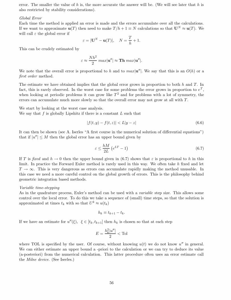
We note that the overall error is proportional to h and to max|u′′|. We say that this is an O(h) or afirst order method.

The estimate we have obtained implies that the global error grows in proportion to both h and T . Infact, this is rarely observed. In the worst case for some problems the error grows in proportion to eT ,when looking at periodic problems it can grow like T 2 and for problems with a lot of symmetry, theerrors can accumulate much more slowly so that the overall error may not grow at all with T .

We start by looking at the worst case analysis.We say that f is globally Lipshitz if there is a constant L such that

|f(t, y) − f(t, z)| < L|y − z| (6.6)

It can then be shown (see A. Iserles “A first course in the numerical solution of differential equations”)that if |u′′| ≤ M then the global error has an upper bound given by

ε ≤hM

2L

(

eLT − 1)

(6.7)

If T is fixed and h → 0 then the upper bound given in (6.7) shows that ε is proportional to h in thislimit. In practice the Forward Euler method is rarely used in this way. We often take h fixed and letT → ∞. This is very dangerous as errors can accumulate rapidly making the method unusable. Inthis case we need a more careful control on the global growth of errors. This is the philosophy behindgeometric integration based methods.

Variable time-steppingAs in the quadrature process, Euler’s method can be used with a variable step size. This allows somecontrol over the local error. To do this we take a sequence of (small) time steps, so that the solution isapproximated at times tk with so that Uk ≈ u(tk)

hk ≡ tk+1 − tk.

If we have an estimate for u′′(ξ), ξ ∈ [tk, tk+1] then hk is chosen so that at each step

E =h2

k|u′′|

2< Tol

where TOL is specified by the user. Of course, without knowing u(t) we do not know u ′′ in general.We can either estimate an upper bound a -priori to the calculation or we can try to deduce its value(a-posteriori) from the numerical calculation. This latter procedure often uses an error estimate callthe Milne device. (See Iserles.)

56

%%%%%%%%%%%%%%%%%%%%%%%%%%%%%%%%%%%%%%%%%%%%%%%%%%%%%%%%%%%%%%%

% %

% Example 1: Use of the Forward Euler Method %

% %

%%%%%%%%%%%%%%%%%%%%%%%%%%%%%%%%%%%%%%%%%%%%%%%%%%%%%%%%%%%%%%%

%%%%%%%%%%%%%%%%%%%%%%%%%%%%%%%%%%%%%%%%%%%%%%%%%%%%%%%%%%%%%%%

% %

% Consider the ODE du/dt = -2t u^2, u(0) = 1 %

% ========================== %

% %

% This has the solution u(t) = 1/(1 + t^2) %

% ================== %

% %

% So that u(1) = 1/2 %

% %

%%%%%%%%%%%%%%%%%%%%%%%%%%%%%%%%%%%%%%%%%%%%%%%%%%%%%%%%%%%%%%%

%%%%%%%%%%%%%%%%%%%%%%%%%%%%%%%%%%%%%%%%%%%%%%%%%%%%%%%%%%%%%%%

% %

% We can solve this using the Forward Euler method with %

% step size h, to find a numerical approximation U for u(1) %

% %

%%%%%%%%%%%%%%%%%%%%%%%%%%%%%%%%%%%%%%%%%%%%%%%%%%%%%%%%%%%%%%%

%

% Do a series of runs with h reducing in size

%

h = 1;

j = 1;

while j < 8

h = h/2;

%

% Number of time steps

%

N = 1/h + 1;

U = zeros(1,N);

t = zeros(1,N);

U(1) = 1;

t(1) = 0;

for i=2:N

%

% Euler step

%

57

t(i) = h + t(i-1);

U(i) = U(i-1) - 2*h*t(i-1)*U(i-1)^2;

end

hh(j) = h;

%

% Error

%

er(j) = U(N)-1/2;

j = j+1;

end

A = [hh’ er’]

plot(hh,er)

-----------------------------------------------------------------------------------

%

% The resulting solution has the following form

%

>> eul

A =

0.5000 -0.2500

0.2500 -0.1209

0.1250 -0.0591

0.0625 -0.0293

0.0312 -0.0146

0.0156 -0.0073

0.0078 -0.0036

>> h Error

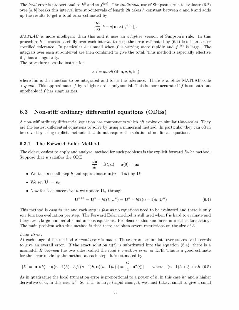
We can see from this that when h is halved, so is the error. The resulting solution for two values of his given below.

6.3.2 The Runge-Kutta method.

A much more locally accurate method is the Runge-Kutta method. Its most famous form is called theexplicit fourth order Runge-Kutta or the RK4 method. Suppose that the ODE is du

dt= f(t,u). Then if

58

0 0.1 0.2 0.3 0.4 0.5 0.6 0.7 0.8 0.9 10.2

0.3

0.4

0.5

0.6

0.7

0.8

0.9

1

h=0.25

h = 0.0078

Exact

t

u

Figure 6.1: Solution of the Forward Euler Method

0 0.1 0.2 0.3 0.4 0.5−0.25

−0.2

−0.15

−0.1

−0.05

0

h

Error

Figure 6.2: Error of the Forward Euler method as a function of h

we know Un, and set t = (n − 1)h the value of Un+1 is given by the sequence of operations

k1 = hf(t,Un)

k2 = hf

(

t +h

2, Un +

k1

2

)

k3 = hf

(

t +h

2, Un +

k2

2

)

k4 = hf(t + h, Un + k3)

Un+1 = Un +1

6(k1 + 2k2 + 2k3 + k4)

It can be shown that there is a value C which depends on f in a complex way such that a local truncationerror E = |u(t + h) −Un+1| is bounded by

E ≤ Ch5

Over a large number of steps these errors accumulate as before to give a global error ε of the form:

ε ∼ C(eLT − 1)h4

The error is proportional to h4. Hence the name an order 4 method. The error for a given h is muchsmaller than for the Forward Euler method. This method is VERY widely favoured as

59

1. It is easy to use and no equations need to be solved at each stage.

2. It is highly accurate for moderate h values

3. It is a one step method i.e. Un+1 only depends on Un

4. It is easy to start and easy to code.

For many people it is the ONLY method they ever use!! However, it has certain disadvantages.

1. The function f must be evaluated four times at each iteration. This may be difficult if f is hardor expensive to evaluate.

2. Errors accumulate rapidly as T increases.

3. The method cannot be used for stiff problems unless h is very small.

%%%%%%%%%%%%%%%%%%%%%%%%%%%%%%%%%%%%%%%%%%%%%%%%%%%%%%%%%%%%%%%

% %

% Example 2: Use of the 4th Order Runge-Kutta method %

% %

%%%%%%%%%%%%%%%%%%%%%%%%%%%%%%%%%%%%%%%%%%%%%%%%%%%%%%%%%%%%%%%

%%%%%%%%%%%%%%%%%%%%%%%%%%%%%%%%%%%%%%%%%%%%%%%%%%%%%%%%%%%%%%%

% %

% Consider the ODE du/dt = -2t u^2, u(0) = 1 %

% ========================== %

% %

% This has the solution u(t) = 1/(1 + t^2) %

% ================== %

% %

% So that u(1) = 1/2 %

% %

%%%%%%%%%%%%%%%%%%%%%%%%%%%%%%%%%%%%%%%%%%%%%%%%%%%%%%%%%%%%%%%

%%%%%%%%%%%%%%%%%%%%%%%%%%%%%%%%%%%%%%%%%%%%%%%%%%%%%%%%%%%%%%%

% %

% We can solve this using the RK4 method with %

% step size h, to find a numerical approximation for u(1) %

% %

%%%%%%%%%%%%%%%%%%%%%%%%%%%%%%%%%%%%%%%%%%%%%%%%%%%%%%%%%%%%%%%

%%%%%%%%%%%%%%%%%%%%%%%%%%%%%%%%%%%%%%%%%%%%%%%%%%%%%%%%%%%%%%%

% %

% The function is calculated in frk.m %

% %

%%%%%%%%%%%%%%%%%%%%%%%%%%%%%%%%%%%%%%%%%%%%%%%%%%%%%%%%%%%%%%%

%-------------------------------------------------------------%

%%%%%%%%%%%%%%%%%%%%%%%%%%%%%%%%%%%%%%%%%%%%%%%%%%%%%%%%%%%%%%%

% %

% Do a series of runs with h reducing in size %

% %

%%%%%%%%%%%%%%%%%%%%%%%%%%%%%%%%%%%%%%%%%%%%%%%%%%%%%%%%%%%%%%%

60

h = 1;

j = 1;

while j < 8

h = h/2;

%

% Number of time steps

%

N = 1/h + 1;

U = zeros(1,N);

t = zeros(1,N);

%

% Initial values

%

u(1) = 1;

t(1) = 0;

for i=2:N

%

% Runge-Kutta step

%

th = h/2 + t(i-1);

t(i) = h + t(i-1);

k1 = h*frk(t(i-1),U(i-1));

k2 = h*frk(th,U(i-1)+k1/2);

k3 = h*frk(th,U(i-1)+k2/2);

k4 = h*frk(t(i),U(i-1)+k3);

U(i) = U(i-1) + (k1+2*k2+2*k3+k4)/6;

end

hh(j) = h;

%

% Error

%

er(j) = U(N)-1/2;

j = j+1;

end

61

rat = er./hh.^4;

A = [hh’ er’ rat’]

plot(log(hh),log(abs(er)))

>> %%%%%%%%%%%%%%%%%%%%%%%%%%%%%%%%%%%%%%%%%%%%%%%%%%%%%%%%%%%%%%%%%%%%%%%%%%%%%%%

>> %

>> % Test of the Runge-Kutta code

>> %

>> %%%%%%%%%%%%%%%%%%%%%%%%%%%%%%%%%%%%%%%%%%%%%%%%%%%%%%%%%%%%%%%%%%%%%%%%%%%%%%%

>>

>> rung

A =

0.50000000000000 -0.00029847713504 -0.00477563416071

0.25000000000000 0.00001355253692 0.00346944945065

0.12500000000000 0.00000139255165 0.00570389155200

0.06250000000000 0.00000009811779 0.00643024720193

0.03125000000000 0.00000000640084 0.00671176833566

0.01562500000000 0.00000000040734 0.00683396495879

0.00781250000000 0.00000000002567 0.00689065456390

>> % h error error/h^4

>> %

>> % Note that error/h^4 is almost constant

>> %

>> diary off

0 0.1 0.2 0.3 0.4 0.5 0.6 0.7 0.8 0.9 10.5

0.6

0.7

0.8

0.9

1

t

u

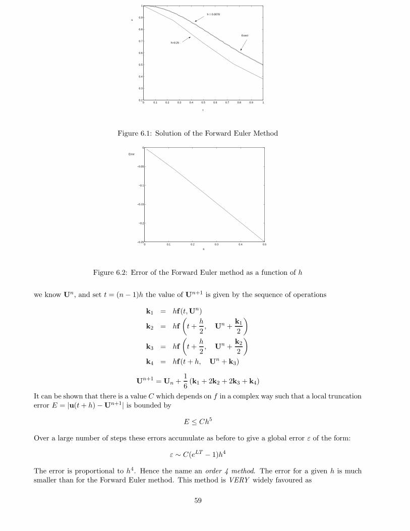
I like to think of the RK4 method as being like a Ford Fiesta. It is easy to use, everyone uses it and it isgood value for money. If you are going to the shops (i.e. solving a relatively straight forward problem)it is the method to use. However, it won’t handle rough country nor would you want it for a very longdrive.To improve the accuracy the RK4 method is often used together with another higher order method toestimate the local error and choose h accordingly. Suppose that the value of Un+1 is given by an RK4method. We could also use a different higher order method to calculate a separate value Un+1. Both

62

Un+1 and Un+1 approximate u(t + h) so that:

Un+1 = u(t + h) + Ch5

Un+1 = u(t + h) + Dh6

Subtracting these estimates we have

‖ Un+1 − Un+1 ‖≤ |C|h5 + |D|h6

If h is small then |C|h5 ≈‖ Un+1 − Un+1 ‖ so the difference between the two calculations gives anestimate for the local error of the RK4 method.We can now use this estimate as follows. Given Un and h

1. Using Un and step size h, calculate Un+1, Un+1 and En+1 =‖ Un+1 − Un+1 ‖.

2. If TOL32 < En+1 < TOL then accept the step

3. If En+1 < TOL32 then set h = 2h and repeat from 1.

4. If En+1 > TOL then set h = h2 and repeat from 1.

This method keeps the local errors below the specified tolerance and also (due to 3) makes an efficientchoice of step size. However it does not control the growth of errors. MATLAB uses such a Runge-Kutta 4,5 pair above the form developed by Dormand & Prince in the ode45 routine. There is a similar(cheaper but less accurate) Runge-Kutta 2,3 pair implemented in the routine ode23. In this routineyou can set both the Absolute Tolerance (as above) or the Relative Tolerance TOL/ ‖ u ‖. You can theode45 routine as follows:

>[t,U] = ode45 (@fun, trange, u_0, options)

Here t is the vector of times at which the approximate solution vector U is given. Because the step-sizeh is chosen at each stage of the algorithm these times will not (necessarily) be equally spaced. Thefunction f(t, u) is specified by ‘fun’ and u0 is the vector of initial conditions. The time interval for thecalculation is given by trange. Setting

trange = [a b]

means that the ode45 routine will integrate the ODE between a and b, giving its output at the (variable)time steps it computes. Alternatively

trange = [a: c: b]

leads to output at the points a, a+ c, a+2c etc. The options command is optional, but it allows controlover the operation of the ode45 routine. In particular you can set the tolerances and/or request statisticson the solution. The options are set by using the odeset routine. For example if you want an absolutetolerance of 10−12 you type

>options = odeset (‘AbsTol’, 1e^(-12}))

By default the absolute tolerance is 10−6 and the relative tolerance is 10−3.

63

%%%%%%%%%%%%%%%%%%%%%%%%%%%%%%%%%%%%%%%%%%%%%%%%%%%%%%%%%%%%%%%

% %

% Example 3: Use of ode45 %

% %

%%%%%%%%%%%%%%%%%%%%%%%%%%%%%%%%%%%%%%%%%%%%%%%%%%%%%%%%%%%%%%%

%%%%%%%%%%%%%%%%%%%%%%%%%%%%%%%%%%%%%%%%%%%%%%%%%%%%%%%%%%%%%%%

% %

% Consider the ODE du/dt = -2t u^2, u(0) = 1 %

% ========================== %

% %

% This has the solution u(t) = 1/(1 + t^2) %

% ================== %

% %

% So that u(1) = 1/2 %

% %

%%%%%%%%%%%%%%%%%%%%%%%%%%%%%%%%%%%%%%%%%%%%%%%%%%%%%%%%%%%%%%%

%%%%%%%%%%%%%%%%%%%%%%%%%%%%%%%%%%%%%%%%%%%%%%%%%%%%%%%%%%%%%%%

% %

% We can solve this using the ode45 method with %

% tolerances 1e-12,to find a numerical approximation for u(1)%

% %

%%%%%%%%%%%%%%%%%%%%%%%%%%%%%%%%%%%%%%%%%%%%%%%%%%%%%%%%%%%%%%%

options=odeset(’AbsTol’,1e-12,’RelTol’,1e-12);

trange = [0:0.05:1];

unit = [1];

[t,U] = ode45(@frk,trange,unit,options);

s = size(U);

err = U(s(1)) - 0.5

6.3.3 The Stormer - Verlet method and geometric integration

Geometric integration is a branch of numerical analysis which aims in part to control global error growthof a numerical approximation over long times. An important application of geometric methods is tosystems of the form

u = vv = −f(u)

}

{

u + f(u) = 0.

More generally, geometric methods can be applied to Hamiltonian systems for which

q = ∂H/∂p, p = −∂H/∂q

For the problem u + f(u) = 0 we set q = u, p = du/dt and

H = p2/2 + F (q) with F =

∫

fdq

64

Multiplying the differential equation by u and integrating with respect to time we find that

H = u2/2 + F (u) = const.

More generally, in an autonomous Hamiltonian system, the Hamiltonian H is a constant for all times.This is an example of a conservation law. Many physical systems conserve particular quantities overall times. An excellent example of this is the solar system considered in isolation with the rest of theuniverse. This obeys a complicated set of differential equations with complex (and indeed chaotic)solutions. However the total energy, angular momentum and linear momentum are conserved for alltime.

To retain the correct dynamics of such a system in a numerical approximation it is essential that thenumerical approximation either exactly conserves the same invariants or (more usually) the approximateequivalent of any conserved quantity varies from a constant by a small but bounded amount for all times.

If this occurs then the approximate solution is likely to be much closer to the true solution for all times.

The Forward Euler method, RK4 and ode45 are not good at preserving such conserved quantities. Forexample if we consider the system

u + f(u) = 0,u2

2+ F (u) = H

An application of the Forward Euler method with U n ≈ u((n − 1)h), V n ≈ u((n − 1)h) gives

Un+1 = Un + hV n, V n+1 = V n − hf(Un)

so thatHn+1 = (V n+1)2

2 + F (Un+1)

= [V n − hf(Un)]2 /2 + F (Un + hV n)

= Hn + h2

2

(

f(Un)2 + (V n)2∂f/∂u)

+ O(h3)

Thus H changes by

Hn+1 − Hn =h2

2

(

f(Un)2 + (V n)2∂f/∂u)

+ O(h3)

at each iteration. If ∂f/∂u > 0 then H is not conserved and increases at each iteration as the errorsaccumulate so that the global error in H grows like nh2. In the RK4 method we have the better resultthat

Hn+1 − Hn = h5Cn.

Again, in general the values of Cn are positive for many problems and the errors in H accumulateover a large number of iterations, with global errors growing like nh5. A widely used method whichavoids many of these problems and has excellent conservation problems is the Stormer - Verlet method(SV) . This is the method of choice for simulations of celestial and molecular dynamics. Not only isit (much) better than RK4 for long-time integrations it is also much cheaper and easier to code up asit only requires one function evaluation per time step. It is also explicit, has global errors O(h2) andit is symmetric. The disadvantage of the SV method is that it can only be used for a certain classof problems (those with a separable Hamiltonian) and it is not a black-box code i.e. it requires somethought to use it. However this is precisely what mathematicians are paid to do!For the problem u + f(u) = 0 the SV method takes the following form

U∗ = Un + h2V n

V n+1 = V n − hf(U∗)

Un+1 = U∗ + h2V n+1

In the SV method we haveHn+1 − Hn = h3Dn.

65

This appears to be worse than RK4. However, unlike RK4 the errors DO NOT accumulate and tendto cancel out. It can be shown that if H is the exact Hamiltonian then

|Hn − H| < Dh3

where D does not depend on n. So, although H is not exactly conserved, the method stays close to itfor all time.We now apply this to an example with f(u) = u3.

66

%%%%%%%%%%%%%%%%%%%%%%%%%%%%%%%%%%%%%%%%%%%%%%%%%

% %

% Example 4: Stormer-Verlet method for %

% %

% u’’ + u^3 = 0, u(0) = 1, u’(0) = 0 %

% %

% In the exact eqn H is constant where %

% %

% H = (u’)^2/2 + u^4/4 %

% %

%%%%%%%%%%%%%%%%%%%%%%%%%%%%%%%%%%%%%%%%%%%%%%%%%

t(1) = 0;

U(1) = 1;

V(1) = 0;

h = 0.1;

H(1) = 1/4;

for i=2:100

Usta = U(i-1) + (h/2)*V(i-1);

V(i) = V(i-1) - h*Usta^3;

U(i) = Usta + (h/2)*V(i);

t(i) = t(i-1) + h;

H(i) = V(i)^2/2 + U(i)^4/4;

end

plot(t,H)

67

−1 −0.8 −0.6 −0.4 −0.2 0 0.2 0.4 0.6 0.8 1−1

−0.8

−0.6

−0.4

−0.2

0

0.2

0.4

0.6

0.8

1

u

v

Figure 6.3: A plot of U, V for the exact and numerical solution

0 1 2 3 4 5 6 7 8 9 100.25

0.252

t

H

Figure 6.4: A plot of H showing the bounded variation

68

6.4 Stiff Differential Equations

6.4.1 Definition

In a stiff differential equation the solution components evolve on very different timescales. This causesa problem as a numerical method, such as ode45, possibly chooses a step size for the most rapidlyevolving component, even if its contribution to the solution is negligable. This leads to very small stepsizes, highly inefficient computations and long waits for the user! The reason for this is an instabilityin the method , where a small error may grow rapidly with each step.

Suppose we want to solve the ODEu = f(u)

and the numerical method makes a small error e. We ask the question, how does e grow during thecalculation? To answer this we start by looking at how a small disturbance to the solution of the ODEchanges. Suppose that e is such a disturbance so that

d

dt(u + e) = f(u + e)

To leading order the perturbation e then satisfies the linear differential equation

du

dt+

de

dt= f(u) + Ae A =

∂f

∂u.

The perturbation growth is thus described by the differential equation

de

dt= Ae where A = ∂f/∂u. (6.8)

Now look at the ODE (6.8). This has the solution

e = eAte0

where e0 is the initial perturbation. So that if A = UΛU−1 then

e = Ue∧tU−1eo.

Alternatively, if A has eigenvalues λi and eigenvectors φi then

Aφi = λiφi φi : eigenvector

Thus if e0 is in the direction of φi so thate0 = aφi

it follows thate(t) = aeλitφi

It follows further that‖ e(t) ‖= |a|eµit ‖ φi ‖

where µi is the real part of λi so that it is the real part of the eigenvalues which control the growth ofsmall perturbations.If |λi| is large and the real part of λi is less than zero, then the contribution to e in the direction ofthe eigenvector φi rapidly decays to zero. After only a short time the perturbation is dominated bythe component in the direction of the eigenvector φj for which λj has the largest real part over all theeigenvalues.We are now able to define what we mean by a stiff system.

DEFINITION

The system is stiff if the matrix A has eigenvalues λi for which

maxj

|λj | � minj

|λj|.

69

Typically, in an application a ratio of over 10 is considered to lead to a stiff systemIn a physical system the components for which |λj | is large, and the real part of λj is negative, decay

rapidly and are not seen in the solution apart from some initial transients. It is therefore somewhatparadoxical that it is precisely these components which lead to instabilities in the numerical scheme.Thisis another way of saying that the solution has components that evolve at very different rates.

6.4.2 Numerical Methods

Now we look at a variety of numerical methods for solving the linear equation (6.8) so that we maycompare the growth of perturbations to the numerical solution with those of the true solution. Firstlook at the performance of the Forward Euler method when applied to this problem. We have

Un+1 = Un + hf(Un)

so thatUn+1 = Un + hAUn = (I + hA) Un

ThereforeUn = (I + hA)n U1

But I + hA has the same eigenvectors φj as A and has eigenvalues

1 + hλj

So, the contribution to Un in the direction of the eigenvector φj grows as

(1 + hλj)n−1

or more precisely as |1 + hλj |n−1. In particular the errors caused by truncation error or by rounding

error only decay if |1 + hλj | < 1 for all λj.We now find an extraordinary paradox. Suppose that λj is real and that

λj = −µ with µ � 1

Theneλj t = e−µt � 1, if t � 1

However|1 + hλj |

n = |1 − µh|n � 1 if µh > 2 and n � 1.

So the most rapidly decaying components of the perturbation to the continuous solution are the com-ponents of Un which are growing most rapidly.

DEFINITION

We say the Forward Euler method with step size h is stable if given a matrix A with eigenvalues λj

with the real part less than zero then |1 + hλj | < 1 for all λj . In particular if λj are all real then themethod is stable only if

h < 2/max|λj |

This is the restriction on h which means that solution errors do not grow. If h is larger than this boundthen errors grow and the method is unstable.

Here we see the problem. A component in the direction of φj with large |λj| and with real part λj < 0dominates the choice of step size even though this component is very small.

70

• The LOCAL (TRUNCATION) ERROR that is made at each stage of the calculation is given by

h2|u′′|

2.

So the error made at each stage depends on the SOLUTION. If all of the eigenvalues of A havenegative real part then this error is ultimately dominated by the component of the solution thatdecays most slowly, which is in turn determinated by the eigenvalue of A with the largest real part.Soi that it is the eigenvalue with the real part closest to zero, and typically this is the eigenvaluewith the smallest modulus.

• In contrast the GROWTH of the error as the iteration proceeds depends on the eigenvalue of Awith the largest modulus, even though this eigenvalue may have a large negative real part andthus not contribute to the solution in any way.

There are therefore two restrictions on h, it must be small both for accuracy at each stage and forstability to stop the errors growing. Stiffness arises when the restriction on h for stability is much moresevere than the restriction for accuracy.

This introduces us to the ideas of stability and instability. It is surprisingly hard to give a precisedefinition of what we mean by instabiliy in a numerical method which accounts for all cases - later on wewill give a precise definition which covers certain cases, but for the present we will have the following.

INFORMAL DEFINITION OF INSTABILITY

A numerical method to solve a differential equation is unstable if the errors it makes (or indeed itssolution) grow more rapidly than the underlying solution. If the errors decay then it is stable.

Exercise Check the definition of stability for the Forward Euler method is consistent with this informaldefinition.

Returning to the Forward Euler example. If h > 0 and λ = p + iq then |1 + hλ| < 1 implies that

(1 + hp)2 + (hq)2 < 1

2hp + h2p2 + h2q2 < 0

2p + hp2 + hq2 < 0.

So that the method is stable if (p, q) lies in the circle of radius 1h shown in Figure 6.5. In this figure

−30 −20 −10 0 10 20 30−30

−20

−10

0

10

20

30

p

q

STABLE

UNSTABLE

Figure 6.5: Stability region for the Forward Euler method

the shaded region shows the values of p and q for which the numerical method is stable. Recall thatthe original differential equation is stable provided that p lies in the half-plane p < 0. The shaded

71

region only occupies a fraction of this half-plane, although the size of the shaded region increases ash → 0. Thus, for a fixed value of h the numerical method will only have errors which do not grow ifthe eigenvalues of A are severely constrained. Unfortunately this is often not the case, particularly indiscretisations of partial differential equations.

6.4.3 The Backward-Euler Method... an A-stable stiff solver

We now look at another method, The Backward Euler Method (also called the BDF1 method). This isgiven by

Un+1 = Un + hf(Un+1)

The backward Euler method is much harder to use than Forward Euler as we must solve an equation(which is usually nonlinear) at each step of the calculation to find Un+1. It has the same order of error.i.e. the global error is proportional to h. If we now apply this to the equation u = Au we have

Un+1 = Un + hAUn+1

This is a linear system which we need to invert to give

Un+1 = (I − hA)−1Un

Now, if the eigenvalues of A are λj , those of (I − hA)−1 are (1 − hλj)−1, with the same eigenvectors.

Exercise: Prove this.

Thus the contribution to Un in the direction of φj evolves as

|1 − hλj |1−n

Now let λj = p + iq as before. It follows that

|1 − hλj |−2 =

1

(1 − hp)2 + (hq)2

Therefore the errors decay and the method is stable if

1

(1 − hp)2 + (hq)2< 1

if 1 < (1 − hp)2 + (hq)2

or 0 < h(p2 + q2) − 2p

The resulting stability region is illustrated (shaded) in Figure 6.6: This picture is in complete contrastto the one that we obtained for the Forward Euler method. The stability region is now very large andcertainly includes the half-plane p < 0. Thus any errors in the numerical method will be rapidly dampedout. Unfortunately the numerical solution can decay even if p ≥ 0, so that neutral or growing termsin the underlying solution can be damped out as well. This is a source of (potential) long term error,especially in Hamiltonian problems.

The Backward Euler method is very reliable and has other nice properties (a maximum principle) whichmake it especially suitable for solving PDEs. The main disadvantage to using it is that we must solvea nonlinear equation to find Un+1. This is an example of the basic principle that there is no suchthing as a free lunch! The penalty of a stable method is the need to do more work. Note, however,that the Stormer - Verlet method is a good approximation to a free lunch. Finding Un+1 when thesystem has a high dimension (e.g.104) is a considerable task, especially as this calculation must be donequickly and often. Usually we use an iterative method such as the Newton-Raphson or Broyden method.Fortunately a good initial guess is available namely a value Un+1 which is obtained by taking one-stepof an explicit method (e.g Forward Euler) applied to Un. This procedure is called a predictor-correctormethod in which the explicit method predicts the value Un+1 which is then corrected (usually by aniterative method) to give Un+1.

72

−30 −20 −10 0 10 20 30−30

−20

−10

0

10

20

30

p

q

STABLE

UNSTABLE 2/h

1/h

Figure 6.6: Stability region for the Backward Euler method.

6.4.4 The Trapezium Rule: a symmetric stiff solver

The Trapezium Rule is given by

Un+1 = Un +h

2[f(Un) + f(Un+1)]

This is another implicit method which needs a function solve at each step to find Un+1 using a predictor-corrector method.It is also a symmetric method i.e. if you know Un and you wish to find Un+1 with step-size h thenthis is the same method for finding Un given Un+1 and step-size −h. This property is important forfinding approximations to the solutions equations such as u + u = 0 which are the same both forwardsand backwards in time.

If we now apply this method to u = Au we have

Un+1 = Un +h

2[AUn + AUn+1]

so that

Un+1 =

(

I −hA

2

)

−1 (

I +hA

2

)

Un

A straight forward calculation of the eigenvalues of the matrix linking Un to Un+1 shows that growthrate of the component in the direction of φj is given by

∣

∣

∣

∣

∣

1 +hλj

2

1 −hλj

2

∣

∣

∣

∣

∣

If we take λ = p + iq then

θ ≡

∣

∣

∣

∣

∣

1 + hλ2

1 − hλ2

∣

∣

∣

∣

∣

2

=

(

1 + ph2

)2+ q2h

2

4

(

1 − ph2

)2+ q2h

2

4

Thus

θ < 1 if

(

1 +ph

2

)2

+ q2 <

(

1 −ph

2

)2

+ q2 i.e if p < 0

The stability region of the numerical method is thus the half-plane p < 0 illustrated in Figure 6.7which is identical to the region of stability of the underlying differential equation. As a consequence thedynamics of the solution of the trapezium rule exactly mirrors the true dynamics. This is an excellentstate of affairs.

73

The local error LTE of the Trapezium Rule is given by:

LTE =h3|u′′′

12.

If h is constant the overall error is then proportional to h2. To estimate the step-size we keep LTE <TOL much as before.

The Trapezium Rule, together with a third order method to control the local error, is implemented inthe MATLAB routine ode23t . Here the (second order implicit) Trapezium Rule is a good one to useif accuracy is not essential. It is very reliable and relatively cheap, but the overall error is quite highcompared to (say) ode45.

−30 −20 −10 0 10 20 30−30

−20

−10

0

10

20

30

p

q

STABLE

UNSTABLE

Figure 6.7: Stability Region for the Trapezium rule and the Implicit Mid-Point rule.

6.4.5 The Implicit Mid-point Rule...an ideal stiff solver?

The implicit mid-point rule is a symmetric Runge-Kutta method closely related to the trapezium rule.It is given by

Un+1 = Un + hf

(

1

2(Un + Un+1)

)

(6.9)

When applied to the linear ODE u′ = Au the method in (6.9) gives exactly the same sequence of iteratesas the trapezium rule check this. Thus its stability properties are identical to the Trapezium Rule andhence are optimal. Like the Trapezium Rule the global error of the Implicit Mid-Point Rule varies ash2 and a function solve is required to find Un+1. It has various other very nice features. In particularit preserves linear and quadratic invariants, so that if u is a solution of the differential equation andthere exists a vector c and a matrix A so that c · u is constant and uT Au is a constant then the sameidentities hold for the discrete solution as well. It is also a symplectic method (like the Stormer- Verletmethod). An example of the usefulness of these properties comes from the computation of the orbitsof the planets in the solar system. A linear invariant of this system is the linear momentum and aquadratic invariant is the angular momentum. Both are exactly conserved by this method, which alsocomes close to conserving the total energy. Great stuff, but at the cost of an expensive function solve.

The Implicit Mid-point rule is the simplest example of a sequence of implicit Runge-Kutta methodscalled Gauss-Legendre methods. If you want to solve an ODE very accurately for long times withexcellent stability, but regardless of cost, then these are the methods to use. Gauss-Legendre methodsare the Lamborghinis of the numerical ODE world.They are expensive and hard to drive, but they havestyle! They are implemented in Fortran in the excellent AUTO code.

74

6.4.6 Multi-step methods

These are the most widely used methods for stiff problems and include Adams and BDF methods andthe Trapezium rule. There is a vast literature on them, see Iserles. Multi-step methods are very flexibleto use and are relatively easy to analyse. They take the form

k∑

l=0

al Un−l = h

k∑

l=0

bl fn−l

where fk = f(tk,Uk), tk = (k − 1)h.To find Un you need to know Un−1, . . . ,Un−k. To start the method given U0 you need to use anothermethod (e.g. RK4) to find U1, . . . Uk−1.

In these methods you use information from previous time steps and (in an explicit method) one functionevaluation to find Un. Thus they are cheaper than RK4 and potentially more accurate. Some propertiesof these methods are as follows.

• The method has order if the truncation error at each stage is given by Chp+1u(p+1) and the overallmethod has error of order p, so that the global error is proportional to hp.

• These methods are implicit if bo 6= 0 and explicit if b0 = 0. Explicit methods give Un directlywhereas implicit methods need an equation to be solved.

• They have “backwards difference form” if bo 6= 0, bl = 0 otherwise

DEFINITION

A multi-step method is A-stable if when used to solve the equation

u′ = Au,

when all eigenvalues of A have negative real part, then |Un| → 0 as n → ∞, for all values of h > 0.More precisely, a method is A-stable if the roots z of the polynomial equation Σalz

−l − hλΣblz−l = 0

have modulus less than or equal to one if the real part of λ is less than or equal to zero.

A-stability is a very desirable property for stiff problems, which the Trapezium Rule has. However, itis almost unique in having this property as the following theorem shows:

THEOREM Only implicit methods of order less than or equal to 2 can be A-stable.

Implicit Multi-step methods involve solving non-linear equations. As before the usual method to dothis is a predictor corrector method namely you generate an approximation U for Un using an explicitpredictor method and then correct this to find Un. An easy corrector is to use an iterative one. Supposewe set Uo

n = Un where Un is a predicted value obtained using an explicit method. We now performthe following iteration to find a sequence of approximations Ur

n to Un:

Urn =

[

−

k∑

l=1

alUr−1n−l + h

∑

blfn−l

]

/ao

wherefk = f(tk,U

r−1k ),

iterating either to convergence or a fixed number of times.

75

As in the Runge-Kutta methods, it is common to use two multistep methods simultaneously. One toperform the numerical solution. The other to give an estimate of the error. In the celebrated Gearsolvers (named after their inventor W.Gear) the method chooses what multi-step method to use at eachstep from a range of methods of different orders (and stability ranges), based on an estimate of the errorfrom the two methods (the latter is called the Milne device).

MATLAB has an excellent stiff Gear solver given by ode15s . It is used in exactly the same way asode45 and is the routine to use for most problems, if you don’t know much about their structure.

***IF YOU LEARN NOTHING ELSE FROM THIS CHAPTER IT IS TO USE ODE15S

An important sub-set of multi-step methods are BDF (backwards difference form) methods. BDFnmethods have order n (global errors proportional to hn) and BDF1 is just the Backwards Error method.The important Fortran ODE code DDASSL and ode15s are both based on BDF methods and theirextensions. The first three BDF methods are given by:

BDF1 : Un −Un−1 = h fn [Backward Euler]BDF2 : Un − 4

3Un−1 + 13Un−2 = 2

3hfnBDF3 : Un − 18

11Un−1 + 911Un−2 −

211Un−3 = 6

11h fn

These methods have excellent stability properties: BDF2 is A-stable (damping out errors but not beingtoo dissipative). BDF3 is A(α) stable rather than A-stable; its stability region includes a wedge of angleα and this includes the eigenvalues of many problems such as those arising in fluid mechanics.BDF methods are the Land Rovers of ODE solvers. They may not be pretty or easy to use, but theywill handle rough country and will nearly always get you where you want to go (although they are notto be used for Hamiltonian problems!).

6.5 Differential Algebraic Equations (DAEs)

An important application of BDF methods is to differential algebraic equations. These equations com-bine algebraic and differential equations and they are VERY common in many applications for example

chemistry, electronics, fluid mechanics and robotics. In a DAE we think of U =[

pq

]

as satisfying the

equations

p = f (p,q), 0 = g (p,q). (6.10)

The second of these equations is the algebraic (or constraint) equation.We will first look at the scalarcase. If we differentiate this with respect to t we have

0 =∂g

∂pp +

∂g

∂qq.

If dg/dq is invertible we then have

q = −

(

∂g

∂q

)

−1 ∂g

∂pp = −

(

∂g

∂q

)

−1 ∂g

∂pf

Thus we arrive at a differential equation for q. We call problems of this form index-1 problems. If wehave to differentiate twice with respect to t to get a differential equation for q we call this an index-2problem, and if three differentiations are needed an index-3 problem. Electronics and chemistry tend tolead to index-1 problems, fluid mechanics to index-2 problems and robotics to index-3 problems. MAT-LAB can handle index-1 problems but has difficulties with problems of a higher index. Full details on

76

the theory and computation of DAEs are given in the very readable book by U. Ascher and L. Petzold.

It is not at all obvious how to apply an explicit method to solve such equations, especially to ensurethat the constraint g(p,q) = 0 is met at each stage.However, it is easy to code these up using a BDF method. For example if we apply BDF2 to the DAE(6.10) we get:

pn − 43 pn−1 + 1

3 pn−2 = 23h f(pn,qn)

0 = g(pn,qn)

As before we have to solve Nonlinear equations to find pn and qn, but these equations are no worse tosolve than before. In ddassl these equations are solved using quasi-Newton methods in which conjugate-gradient methods are used to speed up the linear algebra.

The code ode15s can solve DAEs of the form

Mu = f(u)

Here the matrix M can be singular, for example if

M =

(

1 00 0

)

, f ≡

(

fg

)

and u ≡

(

pq

)

then we have p = f and 0 = g as in (6.10).When using ode15s in this way you specify M in advance and then proceed much as before. Moredetails are given by help ode15s.

77

Chapter 7

Two Point Boundary Value Problems(BVPs)

7.1 Introduction

Two point boundary problems (2pt BVPs) take the form:

u = f(x,u) u ∈ IRn

g1(u(a)) = α x ∈ IRg2(u(b)) = β

where g1,α ∈ IRm and g2,β ∈ IRn−m. Here x is usually thought of as a spatial variable.Two point BVPs arise in many contexts of which the following are examples.

1. They are one-dimensional elliptic equations and arise in their own right as descriptions of physicalproblems. For example, the equation for the deflection of the Euler strut is given by:

d2u/dx2 + λ sin(u) = 0 u(0) = u(1) = 0,

and the equation for rock deformation (see work by CJB and Professor Giles Hunt) by:

d4u/dx4 + Pd2u/dx2 + f(u) = 0, u(0) = u′′(0) = u(1) = u′′(1) = 0

2. As steady states of parabolic or hyperbolic partial differential equations. For example the limit ofthe solutions of

∂u/∂t = ∂u/∂x − f(x, u)

in the limit of t → ∞ [Often a good way to solve the steady state problem is to convert it to sucha time-dependent problem].

3. As travelling wave solutions of partial differential equations or (more generally) as similarityreductions reductions of partial differential equations. (These will be described in the semesterTwo course on Mathematical Modelling.) An example of this is given by the Bergers’ equation:

∂θ

∂t+ θ

∂θ

∂z= ε

∂2θ

∂z2

If we look for a travelling wave solution with

θ(z, t) = u(x) where x = z − ct

78

andθ(−∞, t) = 1, θ(∞, t) = −1.

Then u satisfies the BVP

cdu

dx+ u

du

dx= ε

d2u

dx2

u(−∞) = 1, u(∞) = −1.

which is a two-point boundary value problem.

A special (and very hard) case of two-point BVPs is given when a = −∞ and/or b = ∞. Here we lookfor ground state, homoclinic or heteroclinic solutions. These are very common in PDEs as self-similarsolutions or in quantum mechanics as bound-states We have just seen such a problem in the travellingwave example.

There is a huge difference between BVPs and IVPs. In general an initial value problem always has aunique solution. However a BVP may have one, several (sometimes ∞) or no solutions.The theory of such problems is very subtle. An excellent description of this and of numerical methodsfor them is given in the book on 2pt BVPs by Ascher, Matheij and Russell. There are many methodsfor solving BVPs. These include shooting methods, finite difference methods, finite element methods,spectral methods and collocation methods. The latter are used in the MATLAB code bvp4c andin Fortran codes such as COLSYS, MOVCOL and AUTO. They are especially suitable for use withadaptive and non-uniform meshes. In this course we will look at shooting methods and finite differencemethods.

7.2 Shooting Methods

These are the simplest methods for solving BVPs and are based on using IVP software such as ode15s.They are easy to use and it is often worth trying them first regardless of the nature of the underlyingproblem, although they can perform badly on problems with boundary laters. In a shooting method youreduce the problem to one of finding the correct boundary values. As this is such a neat idea you should:

SHOOT FIRST AND ASK QUESTIONS LATER!

The idea behind shooting methods is simple. Let y be a solution of the initial value problem

dy

dx= f(x,y), y(a) = z ∈ IRn (7.1)

Suppose we take general initial conditions y(a) = z. The initial value problem (7.1) can always besolved for such general values so that y(b) is then a function F(z) of z. If we can find a suitable vectorz so that

g1(z) = α and also g2(F(z)) = β

then we will have found a solution of the corresponding boundary value problem by simply settingu(x) ≡ y(x).

The procedure works as follows

1. At the point x = a we have g1(z) = α. As g1 ∈ IRm this condition fixes m components of thevector z say z1, . . . , zm. The other n − m components (zm+1, . . . , zn) can be chosen freely.

2. Next use an initial value solver such as ode15s to calculate y(b) ≡ F(z).

79

3. To satisfy the boundary conditions we must have g2(F(z)) = β. However, as g2 ∈ IRn−m we haven − m (usually nonlinear) equations to be satisfied for the n − m unknowns zm+1, . . . , zn.These nonlinear equations can be solved using a nonlinear solver such as the Newton-Raphsonalgorithm or a MATLAB routine such as fzero or fminsearch.

Shooting methods perform well for problems without boundary or internal layers. For those withboundary layers the effects of exponentially growing terms make these methods hopelessly ill conditionedand unusable. There are extensions of shooting methods called multi-shooting methods which can beused for problems with boundary layers. However these are very problem dependent and are not easyto use.

Example 1

The easiest example of an application of these methods is to linear boundary value problems of the form

a(x)d2u

dx2+ b(x)

du

dx+ c(x)u = d(x)

with the boundary conditions u(0) = 0, u(1) = 0.We consider the initial value problem

ay′′ + by′ + cy = d (7.2)

with y(0) = z1 and y′(0) = z2

The first boundary condition on u forces z1 = 0. However z2 is arbitrary at this stage.Because of the linearity of (??) it follows that there are constants p and q so that

y(1) = p + qz2

[Exercise: prove this]The values of p and q can be found easily by using an initial value solver applied to (??). For example,if we set z2 = 0 then p = y(1) and if z2 = 1 then q = y(1) − p. The value of z2 for which y(1) = 0 isthen given by

z2 = −p/q.

Example 2

Suppose now that we want to solve the nonlinear boundary value problem

u′′ + u2 = 1, u(0) = u(1) = 0.

as before, we solve the initial value problem

y′′ + y2 = 1, y(0) = z1, y′(0) = z2, (7.3)

with z1 = 0 forced. In this case we havey(1) = F (z2)

where F is a nonlinear function of z2. Applying the second boundary condition, y(1) = 0, it followsthat z2 must satisfy the equation

F (z2) = 0.

The function F (z2) can be computed by using ode15s. This is illustrated below. It is clear that thisfunction has a single root at about z2 = 33.46

80

0 5 10 15 20 25 30 35 40 45 50−8

−6

−4

−2

0

2

4

6

root at 33.4618

z2

f

The code to generate the function F (z2) is given below:

%%%%%%%%%%%%%%%%%%%%%%%%%%%%%%%%%%%%%%%%%

% %

% Shooting code %

% %

%%%%%%%%%%%%%%%%%%%%%%%%%%%%%%%%%%%%%%%%%

function F=funn(x)

[t,u] = ode15s(’u2’,[0 1],[0 x]);

s = size(t);

ss = s(1);

F = u(ss,1);

--------------------------------------------------------

%%%%%%%%%%%%%%%%%%%%%%%%%%%%%%%%%%%%%%

% %

% u’’ + u^2 = 1 %

% %

%%%%%%%%%%%%%%%%%%%%%%%%%%%%%%%%%%%%%%

function f=u2(t,u)

f=zeros(2,1);

f(1) = u(2);

f(2) = 1-u(1)^2;

--------------------------------------------------------

One way to find z2 is to use the MATLAB command fzero given an initial guess of z2 = 30. Noticethe way that this code uses the function funn computerd using ode15s.

>> z2 = fzero(’funn’,30)

z2 =

81

33.4618

The resulting solution u and u′ is illustrated below:

0 0.1 0.2 0.3 0.4 0.5 0.6 0.7 0.8 0.9 1−40

−30

−20

−10

0

10

20

30

40

x

u

du/dx

An alternative method, which exploits the structure of the problem, is to use a Newton-Raphson method.As F (z2) = y(1) it follows that

dF

dz2=

dy(1)

dz2= φ(z2)

where the function φ(x) satisfies the variational equation

φ′′ + 2yφ = 0, φ(0) = 0, φ′(0) = 1.

To use this method we take a guess z(n)2 for z2 and then simultaneously solve the two ODES

y′′ + y2 = 1, y(0) = 0, y′(0) = z(n)2 , φ′′ + 2yφ = 0, φ(0) = 0, φ′(0) = 1,

using ode15s. We then use a Newton-Raphson iteration to improve the guess via the equation

z(n+1)2 = z

(n)2 −

y(1)

φ(1).

This procedure converges rapidly given a reasonable starting guess.

7.3 Finite Difference Methods

7.3.1 Discretising the second derivative.

Finite difference methods aim to to find the solution at all interior points within the interval [a, b].Suppose that we divide up the interval [a, b] into N equal divisions, so that if h = (b − a)/(N − 1) weset xi = a + (i − 1)h i = 1, . . . , N.Now we introduce a vector Ui so that

Ui ≈ u(xi) (7.4)

Now, by using a Taylor series expansion, it follows that

u(xi+1) = u(xi) + hu′(xi) + h2

2 u′′(xi) + . . .

u(xi−1) = u(xi) − hu′(xi) + h2

2 u′′(xi) + . . .

By making a slightly more detailed calculation it follows that

u(xi+1) − 2u(xi) + u(xi−1)

h2= u′′(xi) +

h2

12uiv(xi) + . . . (7.5)

82

We now can use (??) to approximate u′′ by

u′′ ≈Ui+1 − 2Ui + Ui−1

h2≡

δ2

h2Ui (7.6)

where δ2 is the iterated central difference operator. The leading error made in (??) when approximatingu′′ by the iterated central difference is then proportional to h2uiv. Now suppose that A is the tri-diagonalmatrix given by

A =

1 0 . . . 01/h2 −2/h2 1/h2

. . .. . .

. . .

1/h2 −2/h2 1/h2

0 1

,

If the vector U then satisfies the linear system

AU =

αf2...

fN−1

β

where fi ≡ f(xi) (7.7)

then (??) is a discretisation to the second order BVP with Dirichlet boundary conditions which is givenby

u′′ = f(x), u(a) = α, u(b) = β.

If we replace U by u in (??) the expression (??) implies that we would make an error of order h2 ash → 0. Note that the structure of A forces U1 = α and UN = β. The vector U can then be found viathe operation

U = A−1

αf2

fN−1

β

Provided that the problem is not too irregular it can then be shown that in the limit of N → ∞ (h → 0)we have

Ui = u(xi) + O(h2) as h → 0.

The solution of the BVP thus becomes (under discretisation) the problem of solving the linear system(??).If f = [α, f2, . . . , fN−1, β]′ then this can be done in MATLAB via the command A\f .

Whilst this is simple to use it is not especially efficient as the backslash operator does not exploit thespecial tri-diagonal structure of Matrix A. A much more efficient algorithm of complexity O(N) is theThomas algorithm which exploits this structure and is based on the LU decomposition. This algorithmis described in Assignment 4. (Note, use of the MATLAB sparse matrix routines will speed things uphere.)

Efficiency is important as the relatively large error of O(N−2) in this method means that we have totake a large value of N to get a reasonable error estimate. More careful discretisations lead to smallererrors at the expense of more work.

7.3.2 Different boundary conditions

We can extend this idea to BVPs with Neumann boundary conditions. For example the BVP u ′′ = fwith the boundary conditions

u′(a) = α, u(b) = β.

83

Problems such as this arise frequently in models of heat conduction and electrical flow. For example,the boundary condition u′(a) = 0 corresponds to a thermal or electrical insulator. There are many waysto deal with such a derivative boundary condition. In the simplest we approximate

u′(a) by (U2 − U1)/h (7.8)

This will change the matrix A to the tridiagonal matrix

A ≡

−1/h 1/h 0 . . . 01/h2 −2/h2 1/h2

. . .. . .

. . .

1/h2 −2/h2 −1/h2

0 0 1

and we must consider the solution to the linear system:

AU =

αf2...

fN−1

β

(7.9)

The linear equation (??) is then a discretisation of the BVP

u′′ = f u′(a) = α, u(b) = β.

The expression (??) is only accurate to O(h) as an approximation to u′(a). We can improve this byusing the approximation

u′(a) ≈ (4U2 − U3 − 3U1)/2h

Exercise. Show that this expression is accurate to O(h2)

This leads to a slightly different matrix A. Unfortunately the resulting matrix is no longer tri-diagonaland we cannot use the Thomas algorithm to invert it.

A special case of Neumann boundary conditions arises when u′(a) = 0. In this case we can introducea “ghost” point U0 approximating u(a − h). The boundary condition implies that to 0(h3) we haveU0 = U2. At the point x = 0 we have

u′′(a) ≈U0 + U2 − 2U1

h2=

2U2 − 2U1

h2(7.10)

This approximation to u′′(a) is correct to O(h2). (Can you show this?)The resulting matrix A is then given by

A =1

h2

−2 21 −2 1

1 −2 1. . .

. . .

Note that in this case A is tri-diagonal, and we can again solve the linear system by using the Thomasalgorithm.

%%%%%%%%%%%%%%%%%%%%%%%%%%%%%%%%%%%%%%%%%%%%%%%%%%%%%%%%%%%%

84

% %

% Code to solve the Neumann two-point boundary value %

% problem: %

% %

% u’’ = -exp(x), u’(0) = 0, u(1) = 0. %

% %

%%%%%%%%%%%%%%%%%%%%%%%%%%%%%%%%%%%%%%%%%%%%%%%%%%%%%%%%%%%%

%

% Set up the mesh

%

N = 101;

h = 1/(N-1);

x = [0:h:1];

%

% Set up the matrix

%

A = diag(ones(N-1,1),-1) + diag(ones(N-1,1),1) - 2*diag(ones(N,1));

A = A/h^2;

%

% Neumann boundary condition at x = 0

%

A(1,2) = 2/h^2;

%

% Dirichlet boundary condition at x = 1

%

A(N,N-1) = 0;

A(N,N) = 1;

%

% Set up the right hand side

%

f = -exp(x)’;

%

% Modify this to allow for the Dirichlet boundary condition

%

f(N) = 0;

85

%

% Solve the system (without using the Thomas algorithm)

%

U = A\f;

%

% Plot the solution

%

plot(x,U)

0 0.1 0.2 0.3 0.4 0.5 0.6 0.7 0.8 0.9 10

0.1

0.2

0.3

0.4

0.5

0.6

0.7

0.8

0.9

x

U(x) Neumann condition

Dirichlet condition

A second example of differential equations occurs for BVPs with periodic boundary conditions for whichu(a) = u(b) and u′(a) = u′(b). Periodic boundary conditions often arise when looking at those BVPsthat describe the travelling wave solutions of hyperbolic equations. They also arise naturally whensolving BVPs on circles or spheres. A natural example of the latter being weather forecasting on thewhole globe. Often BVPs with periodic boundary conditions are solved using spectral methods in whichthe solution is expressed as a combination of trigonometric functions. However they can also be solvedby using finite difference methods. Exploiting periodicity we have

u′′(a) ≈u(a + h) + u(a − h) − 2u(a)

h2=

u(a + h) + u(b − h) − 2u(a)

h2(7.11)

which we approximate by

u′′(a) ≈U2 + UN−1 − 2U1

h2

Setting U = [U1, . . . , UN−1]′ (noting that U1 = UN ) the resulting matrix A is given by

A =

−2/h2 1/h2 0 . . . 0 1/h2

1/h2 . . .. . . 0

0. . .

. . .

1/h2 . . . . . . 1/h2 −2/h2

The resulting discretisation of u′′ then has an error of O(h2) as before. The matrix A is not tri-diagonal,but its special periodic structure means that it can be inverted quickly by using the FFT.

86

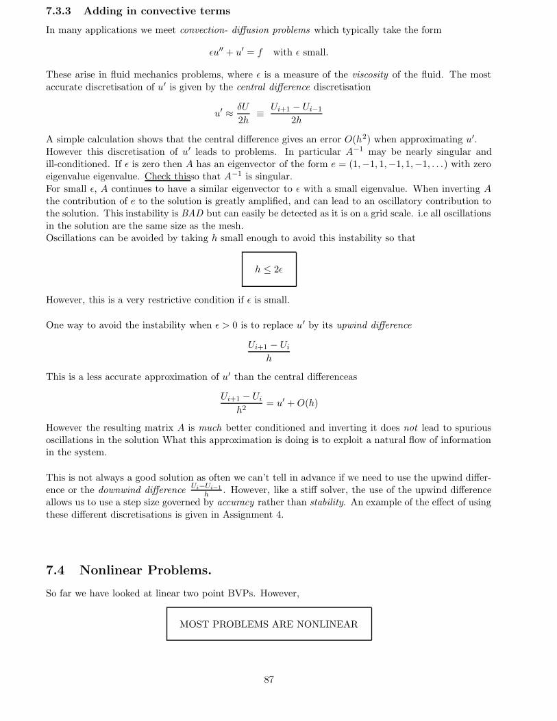
7.3.3 Adding in convective terms

In many applications we meet convection- diffusion problems which typically take the form

εu′′ + u′ = f with ε small.

These arise in fluid mechanics problems, where ε is a measure of the viscosity of the fluid. The mostaccurate discretisation of u′ is given by the central difference discretisation

u′ ≈δU

2h≡

Ui+1 − Ui−1

2h

A simple calculation shows that the central difference gives an error O(h2) when approximating u′.However this discretisation of u′ leads to problems. In particular A−1 may be nearly singular andill-conditioned. If ε is zero then A has an eigenvector of the form e = (1,−1, 1,−1, 1,−1, . . .) with zeroeigenvalue eigenvalue. Check thisso that A−1 is singular.For small ε, A continues to have a similar eigenvector to ε with a small eigenvalue. When inverting Athe contribution of e to the solution is greatly amplified, and can lead to an oscillatory contribution tothe solution. This instability is BAD but can easily be detected as it is on a grid scale. i.e all oscillationsin the solution are the same size as the mesh.Oscillations can be avoided by taking h small enough to avoid this instability so that

h ≤ 2ε

However, this is a very restrictive condition if ε is small.

One way to avoid the instability when ε > 0 is to replace u′ by its upwind difference

Ui+1 − Ui

h

This is a less accurate approximation of u′ than the central differenceas

Ui+1 − Ui

h2= u′ + O(h)

However the resulting matrix A is much better conditioned and inverting it does not lead to spuriousoscillations in the solution What this approximation is doing is to exploit a natural flow of informationin the system.

This is not always a good solution as often we can’t tell in advance if we need to use the upwind differ-ence or the downwind difference Ui−Ui−1

h . However, like a stiff solver, the use of the upwind differenceallows us to use a step size governed by accuracy rather than stability. An example of the effect of usingthese different discretisations is given in Assignment 4.

7.4 Nonlinear Problems.

So far we have looked at linear two point BVPs. However,

MOST PROBLEMS ARE NONLINEAR

87

An important class of nonlinear two point BVPs (called semilinear problems) take the form

a(x)u′′ + b(x)u′ + f(x, u) = 0, (7.12)

and we need to develop techniques to solve them. Two examples of such problems are given by thedifferential equation

u′′ + eu/(1+u) = 0, u(a) = u(b) = 0

which models combustion in a chemically reacting material, and

u′′ +2

xu′ + k(x)u5 = 0, u′(0) = 0, u(∞) = 0, u > 0,

which describes the curvature of space by a spherical body.

A special case is given by the equation

u′′ + f(u) = 0, u(a) = α, u(b) = β. (7.13)

Discretising the differential equation (??) leads to a set of nonlinear equations of the form

AU + f(U) = 0 (7.14)

where A is the matrix given earlier and the vector f is given by

fi ≡ f(Ui).

As with most nonlinear problems, we solve this system by iteration starting with an initial guessalthough, be warned, the system may have one, none or many solutions. Perhaps the most effectivesuch method is the Newton-Raphson algorithm. Suppose that U (n) is an approximate solution of (??),we define the residual R(n) by

AU (n) + f(U (n)) = R(n). (7.15)

The size of Rn is a measure of the quality of this solution.

Now if we define the Jacobian of the nonlinear function f by

Jij = ∂fi/∂Uj

the “linearisation” L of (??) acting on a vector ϕ is given by

Lϕ ≡ Aϕ + Jϕ.

The Newton-Raphson iteration updates U (n) to U (n+1) via the iteration

U (n+1) = U (n) − L−1R(n)

Here the vector W ≡ L−1R(n) can be found by solving the linear system

AW + JW = R(n).

This algorithm converges rapidly (often in about 5 iterations) if the initial guess U (0) is close to the truesolution. Finding such an initial guess can be difficult for a general problem and often requires somea-priori knowledge of the solution.

The Fortran code AUTO uses the Newton-Raphson method coupled to a path-following (homotopy)method to find the solution of a version of the nonlinear systems arising from discretisations of nonlinearBVPs obtained by using collocation.

88

7.5 Other methods

At present collocation is the best method for solving 2pt BVPs. This is a bit like the Finite differencemethod but uses much higher order polynominals. It is also closely related to implicit Runge-Kuttamethods. However, the collation method has no easy extension to higher dimensions. In higher dimen-sions two-point BVPs generalise to elliptic partial differential equations. For such problems the finiteelement method is the mainly used solution procedure, although spectral methods are widely used forproblems with a relatively simple geometry e.g. weather forecasting on the sphere.

CJB 2006

89