machine computation using the exponentially …lipton/may-27-m2as-web-w-figures.pdf · machine...

Machine Computation Using the Exponentially Convergent

Multiscale Spectral Generalized Finite Element Method ∗

Ivo Babuska† Xu Huang‡ Robert Lipton§

May 28, 2013

Abstract

A multiscale spectral generalized finite element method (MS-GFEM) is presented for thesolution of large two and three dimensional stress analysis problems inside heterogeneous media.It can be employed to solve problems too large to be solved directly with FE techniques andis designed for implementation on massively parallel machines. The method is multiscale innature and uses an optimal family of spectrally defined local basis functions over a coarse grid.It is proved that the method has an exponential rate of convergence. To fix ideas we describe itsimplementation for a two dimensional plane strain problem inside a fiber reinforced composite.Here fibers are separated by a minimum distance however no special assumption on the fiberconfiguration such as periodicity or ergodicity is made. The implementation of MS-GFEMdelivers the discrete solution operator using the same order of operations as the number offibers inside the computational domain. This implementation is optimal in that the number ofoperations for solution is of the same order as the input data for the problem. The size of theMS-GFEM matrix used to represent the discrete inverse operator is controlled by the scale ofthe coarse grid and the convergence rate of the spectral basis and can be of order far less thanthe number of fibers. This strategy is general and can be applied to the solution of very largeFE systems associated with the discrete solution of elliptic PDE.

Keywords Generalized Finite Elements, Multiscale method, Spectral method, Heterogeneousmedia, Fiber reinforced composites

AMS Subject Classifications: 65N30, 74S05, 74Q05

1 Introduction

Over the past two hundred years there has been a sustained effort to develop quantitative theoriesfor the analysis of multi-scale phenomena. The early investigations of Poission [46] (1822) sought torepresent the physical response of heterogeneous media by an “equivalent” homogeneous one. Thesubsequent work of Mosotti (1850) [36], Maxwell (1873) [37], and Rayleigh (1892) [47] proposedmethods for recovery of effective coefficients. It is interesting to note that this intense activityoccurred a full century before the mathematical development of homogenization theory for partialdifferential equations in the 1960’s. A survey of the nineteenth and early twentieth century literature

∗To Appear in Mathematical Modeling and Numerical Analysis (M2AN) 2013. Thiswork is supported by grants: NSF DMS-1211014, NSF DMS-1211066, and NSF EPSCOR Cooperative AgreementNo. EPS-1003897 with additional support from the Louisiana Board of Regents†Institute for Computational Engineering and Science and Department of Aerospace Engineering, University of

Texas, Austin, TX 78712([email protected]).‡Department of Mathematics, Louisiana State University, Baton Rouge, LA 70803([email protected]).§Department of Mathematics and Center for Computation and Technology, Louisiana State University, Baton

Rouge, LA 70803([email protected]).

1

Machine Computation using MS-GFEM 2

on this topic is given in the 1926 review paper of Lichternecker [34]. New engineering challengesmotivated by the technology of the mid 20th century brought research activity to bear on structuraland transport properties of heterogeneous media including multiphase polymer systems [13], catalyticmaterials [52], and fiber reinforced composites [26], [28], [29], [18], and [2]. The mathematical theoryof homogenization embodied in the notion of G-convergence can be traced to the work of DeGiorgi([49] example page 661) and the work of Spagnolo [49], [50]. More recent theory addresses problemswith non-symmetric coefficients and the notion of H-convergence, [41]. Homogenization theory forperiodic media and extensions to many important problems in mathematical physics are developedin the work of [12], [16], [48]. The modern mathematical theory of effective coefficients and theirrelation to microstructure has seen explosive development since the late 1980’s and reviews of manyimportant developments can be found in the recent monographs [40] and [56].

Modern computational technology is driving the development of numerical approaches to multi-scale problems. These approaches have gained traction in the applications and the last 40 years haswitnessed a growing scientific literature addressing the numerical treatment of multiscale problems.The field has grown such that it is not possible to provide an exhaustive review within this paper.Here we refer to the recent monograph [21] for an extensive survey of this growing literature. Con-temporary approaches to numerical multi-scaling can be split into two categories, exemplified by (1)Variational Multiscale Methods (VMS) and (2) Multiscale Finite Element Methods (MsFEM).

The scheme behind (VMS) [33] is to (a) additively decompose the solution space VR into fine andcoarse scale contributions, (b) solve the fine scale equations as driven by the coarse scale residual, (c)use the fine scale solution operatorM to eliminate the fine scale solution and represent it as a linearfunction of the coarse scale residual and (d) solve this modified problem over the coarse scale space.Here M is referred to as the reconstruction operator [19], [20] or as the fine scale Green’s function[32]. The operator M is naturally related to the corrector appearing in homogenization theory[42]. In discrete implementations the space VR is the usual finite element (FE) space obtainedon refining the grid associated with the FE coarse scale space VC . Elements of the fine scalespace VF ⊂ VR are chosen to have compact support and taken to be orthogonal to VC in the H1

0

inner product. To fix ideas the coarse scale space is spanned by hat functions associated with thecoarse mesh. In this scheme it is seen that higher fidelity approximations to the nonlocal solutionoperatorM are obtained by redefining VF to include functions with progressively larger support sets(oversampling). Adaptive oversampling methods within the frame work of VMS are introduced anddeveloped in [42], [35]. Recently novel approximation methods have been introduced that providerigorous convergence rates for multiscale methods and are appropriate for the VMS scheme [43],[15], [44]. The use of harmonic coordinates [43] and the transfer property of the flux norm [15],and its localization [44] turn out to provide explicit rates of convergence for multi-scale methods ofVMS type. For VMS posed over the coarse scale mesh of diameter H a convergence rate of O(H) isseen to follow from suitable oversampeling [44]. The reader is also referred to the recent papers [35]for discussion of convergence rates for VMS and dependence on the support of the fine scale basisfunctions. Related but independent developments in multiscale approaches exploiting the interplaybetween local and global computation and homogenization theory are put forth in the HeterogeneousMultiscale Methods introduced in [19] and [20], and [24].

The idea behind (MsFEM) is to consider a coarse mesh with dimensions larger than the het-erogeneity of the medium and instead of using linear or polynomial FE basis functions one usesa finite dimensional space of local solutions to the problem over each element of the coarse mesh.This method has two components to it. The first is to create a local approximation space over eachcoarse element of the mesh and the second requires one to ”paste” these elements together. Thisidea was suggested within the Partition of Unity Method (PUM) for pasting together local approx-imations and analyzed in one dimension in [10] and for higher dimensional problems using speciallocal solutions in [6] and generalized broadly see, [9], [38], [54], [21] and the citations given there.This idea but with a different strategy for pasting together local bases is proposed in [22], [23] andis analyzed in generality there. To illustrate the ideas developed in [22], [23] consider a problem intwo dimensions and let ω be a triangular or quadrilateral element. Here have the following three


basic choices for the construction of the local function space inside ω.

1. Linear boundary data. We retain linearity at the boundary of the element ∂ω and generatelocal shape functions as solutions of the homogenous multiscale equation inside the elementwith boundary conditions on ∂ω associated with linear or bilinear FE. We point out there isa loss of accuracy in this approach since the trace of the exact solution over the boundary ofthe element is not well approximated by a linear function.

2. Better boundary approximation. To improve the boundary approximation over ∂ω we firstsolve a one dimensional problem on every edge of ω with boundary condition on the verticestaken to be the nodal values of FE functions. Typically the equation on each edge of theelement is the restriction of the two dimensional problem to that edge. This approach leadsto better accuracy and both approaches 1) and 2) deliver conforming elements.

3. Oversampling. Let ω∗ be the triangle (quadrilateral) ω enlarged by a factor of 2. Here we takeω ⊂ ω∗ to be concentric and the diameter of ω∗ is twice that of ω. We prescribe the traces ofthe linear FE shape functions on boundary of ω∗. Using this boundary data we solve the localproblem over ω∗. The local approximation is then obtained on restricting these solutions toω. Here this approach leads to nonconforming elements. This approach to constructing localbases is referred to as oversampling [21].

Each approach listed above is a generalization of the linear FEM. It is evident that these methodsimmediately extend if one applies higher order FE boundary conditions on the edges and providesa corresponding higher order MsFEM. Several variations of these ideas have been applied and de-veloped for multiscale problems and an overview of recent literature is given in [21].

We may also interpret MsFEM as a domain decomposition method. Here the elements ω appear-ing in the MsFEM could be understood as a domain decomposition of the computational domain Ω,over which the problem is formulated. The methods 1) and 2) listed above are domain decomposi-tions without overlap and can be understood as a simple mortar method. For further developmentsof the mortar approach to multiscale problems and significant generalizations along these lines see[1]. While the approach 3) employs oversampling and this delivers a domain decomposition withoverlap.

We continue with the theme of domain decomposition and cover Ω with domains ωi such that∪iωi = Ω. The multiscale approach has two components: 1) Local Approximation. On every ωi wepropose m dimensional spaces Vi ⊂ H1(ωi) such that the exact solution u for the multiscale problemcan be well approximated by a function vi ∈ Vi over the element ωi such that ‖ u− vi ‖E(ωi)

≤ εi. 2)

Construction of a H1(Ω) global approximation from local approximations. Here we suppose we haveemployed a scheme (e.g. partition of unity) for ”pasting” the functions vi together to construct a“continuous” function v belonging to H1(Ω) and∑

i

‖ u− v ‖2E(ωi)≤ C

∑ε2i (1.1)

where ‖ · ‖E(ωi) is the energy norm over the element ωi and C independent of u and vi. As inthe case of MsFEM one must also address the dual issues of finding accurate local approximationsand the problem of combining these in an appropriate way to obtain a global approximation to thesolution u. Here the local functions could be pasted or combined to form a global function usingnon-overlapping or overlapping elements.

The Generalized Finite Element Method (GFEM) is an overlapping domain decompositionmethod where global approximations are obtained by pasting together local approximations througha partition of unity. Partition Unity Methods (PUM) originated in [6] and were further extendedand analyzed in [4], [38], [9], [5] and applied to multiscale problems in [54], [3], [55], [25], [53]. TheGFEM utilizes the results of independent local computations carried out across the computationaldomain. The GFEM is constructed by covering the computational domain Ω by a collection of


preselected subsets ωi, i = 1, 2, ..n and constructing finite dimensional approximation spaces Ψi overeach subset using local information. The global approximation is constructed by pasting the localapproximations together using the partition of unity functions subordinate to the covering ωini=1.Since each space Ψi is computed independently the full “global” solution is obtained by solvinga global (macro) system which is an order of magnitude smaller than the system correspondingto a direct application the finite element method to the full structure. This provides an opportu-nity for the significant reduction of the computational work involved in the numerical modeling oflarge heterogeneous problems. Several advantages for applying this strategy to compute fields insideheterogeneous media are listed below:

1. Solution of a global problem with drastically reduced degrees of freedom.

2. Independent local mesh generation versus the generation of a globally defined mesh.

3. Completely independent parallel computation of local problems.

Recent work [7] identifies optimal local finite dimensional approximation spaces Ψi for rough (L∞)coefficients. These new approximation spaces, related to the spectra of restriction operators, provideexponential accuracy in terms of the local degrees of freedom dim(Ψi). This means that to achievea global approximation error of τ with respect to the energy norm one needs to employ lnd+1 ( 1

τ )local basis functions on each subdomain. This newfound low dimensionality for special local approx-imation spaces expands the potential for high fidelity machine computation of elastic fields insidevery large multiscale heterogeneous structures. The crucial aspect of our approach is that it allowsfor the solution of problems that are too large to solve using traditional FEM discretizations on agiven computational resource. This type of approach developed here and in [7] is called MultiscaleSpectral GFEM.

In related work local bases are defined for any shape regular mesh of size H with O(H) conver-gence rate using lnd+1 1

H bases functions per nodal point [27]. Here construction of the near fieldcomponents of the local bases parallels the work of [44], [35] while the far field bases componentsare motivated by the approximants developed in the theory of H-matrices [14]. The optimality ofthis type of local basis remains to be established.

In this paper we address the elastic problem and introduce the appropriate optimal local approx-imation spaces. As in [7] the best choice of local approximation is motivated by the Kolomoragovn-width and we use it to identify and prove the existence of spectrally defined finite dimensionaloptimal local approximation spaces. In doing so we establish the existence of an explicitly definedoptimal local approximation space for this problem. We also provide an estimate to show that it ispossible to achieve a local approximation error of τ with respect to the energy norm using at mostlnd+1( 1

τ ) local basis functions see, section 7. We point out that numerical experiments show that theapproximation error can actually be achieved using far less local basis functions in the pre-asymptoticregime see, [55]. With these estimates in hand the current paper addresses the numerical implemen-tation of Multiscale Spectral GFEM (MS-GFEM) for a fiber reinforced composite medium. For thiscase we identify the relevant error estimate in section 5 and estimates for machine time required forconstructing an approximate solution within a prescribed tolerance τ using a parallel computer in 6.Moreover the size of the MS-GFEM matrix used to represent the discrete inverse operator is smallon the order of ln2(d+1)( 1

τ ). Along the way we identify open problems in elliptic regularity theoryand challenges facing numerical implementation on large parallel computers. We show how theseissues influence our ability to carry out machine computation for very large multiscale problems asexemplified by the composite example treated here.

2 The fiber composite problem

The over all methodology formulated in this paper is quite general and applies to mathematicalformulations of linear elasticity described by measurable tensor valued coefficients. Such generality


is required for the development of mathematically rigorous solution strategies. On the other hand themachine computation of displacement fields inside engineering materials requires a precise descriptionof the heterogeneous material properties. We begin with the general formulation of the equilibriumproblem for an anisotropic heterogeneous linearly elastic medium and then specialize our treatmentto two dimensional plane strain problems for uni-directional fiber reinforced composites.

Let Ω ∈ Rd, d = 2, 3 be a bounded domain with Lipschitz boundary ∂Ω. We start by formulatingthe problem for the system of linear elasticity used for the determination of elastic displacement fieldsu0 : Ω 7→ Rd. The equilibrium equation of linear elasticity is given by

−div(A(x)e(u0(x))) = f(x), x ∈ Ω. (2.1)

Where e(u0) is the elastic strain and is the symmetric part of the gradient of the displacement ∇u0

given by e(u0) = (∇u0 + ∇uT0 )/2. The elasticity tensor of an anisotropic heterogeneous mediumis characterized by a measurable tensor valued field Aijkl(x) ∈ L∞(Ω) for i, j, k, l = 1, d. Aijkl =Aijlk = Ajikl = Aklij . We suppose the tensor satisfies the standard coercivity and boundednessconditions and for any symmetric d× d matrix e

α | e |2≤ Ae : e ≤ β| e |2,x ∈ Ω (2.2)

where Ae : e = Aijkleijekl, and | e |2= e2ij . For this choice of elasticity coefficient the solution is

sought in the Sobolev space H1(Ω;Rd) and the right-hand side (the body force) lies in the dualspace H1(Ω;Rd)∗.

The mathematical formulation of our physical problem is a boundary value problem for thestrongly elliptic system given by the linear elastic system (2.1). The weak solution is formulated inthe standard variational way. We introduce the “energy” bilinear form

B(u,v) =

∫Ω

Ae(u) : e(v)dx,u,v ∈ H1(Ω;Rd), (2.3)

and the energy norm‖ u ‖E(Ω)= (B(u,u))1/2. (2.4)

By E(Ω) we define the energy space given by the quotient space H1(Ω;Rd)/R equipped with theenergy norm. Here the linear space of rigid motions R is given by

R = a + b ∧ x; a and b, in Rd. (2.5)

In what follows we will write B(u,v) = (u,v)E(Ω).Let F1(v) =

∫∂Ω

v · g dx, be the functional of the tractions and F2(v) =∫

Ωf · v dx, be the load

functional. We assume that the natural consistency condition between F1 and F2 given by

F1(v) + F2(v) = 0, for all v ∈ R (2.6)

is satisfied.The elastic displacement field u0 in Ω is the solution of the problem, u0 ∈ E(Ω),

B(u0, v) = F (v) =F1(v) + F2(v),∀v ∈ E(Ω), (2.7)

and is uniquely specified up to a rigid motion. If additionally on Γ ⊂ ∂Ω the boundary condition isu = uΓ then the unique solution u0 ∈ E(Ω),u0 = uΓ satisfies B(u0,v) = F (v),∀v ∈ E(Ω), v = 0on Γ. If F2 = 0 then u0 is the A-harmonic function satisfying B(u0,v) =0,∀v ∈C∞0

The solution of a particular physical problem requires the specialization of the general formulationto the case at hand. Here we focus on the physical problem of calculating stresses and strains insidea uni-directional carbon fiber epoxy resin composite. This type of structural composite is commonlyused in commercial aircraft and wind turbines primarily due to its high specific stiffness and strength.The objective of this paper is to describe the problem of numerical calculation of local fields inside


engineering composite systems. The goal is to highlight the issues and problems related to machinecomputation of local fields inside structural composites typically requiring 108 degrees of freedomper square centimeter of fibrous composite material.

We formulate a deterministic two dimensional elasticity problem for a uni-directional fiber rein-forced composite. It is assumed that the fiber positions and diameters are available through imagedata. In the two dimensional formulation we make the idealization and assume that the fiber crosssections are are circular. In actuality the fibers are more like deformed cylinders. Here we emphasizethat the fiber distribution is not periodic, so that the theory and computational analysis based onthe assumption of a periodicity or almost periodicity characterized by an elastic tensor field of thetype A(x,x/ε) where the tensor field A is smooth in the first variable periodic and oscillatory in thesecond variable cannot be used.

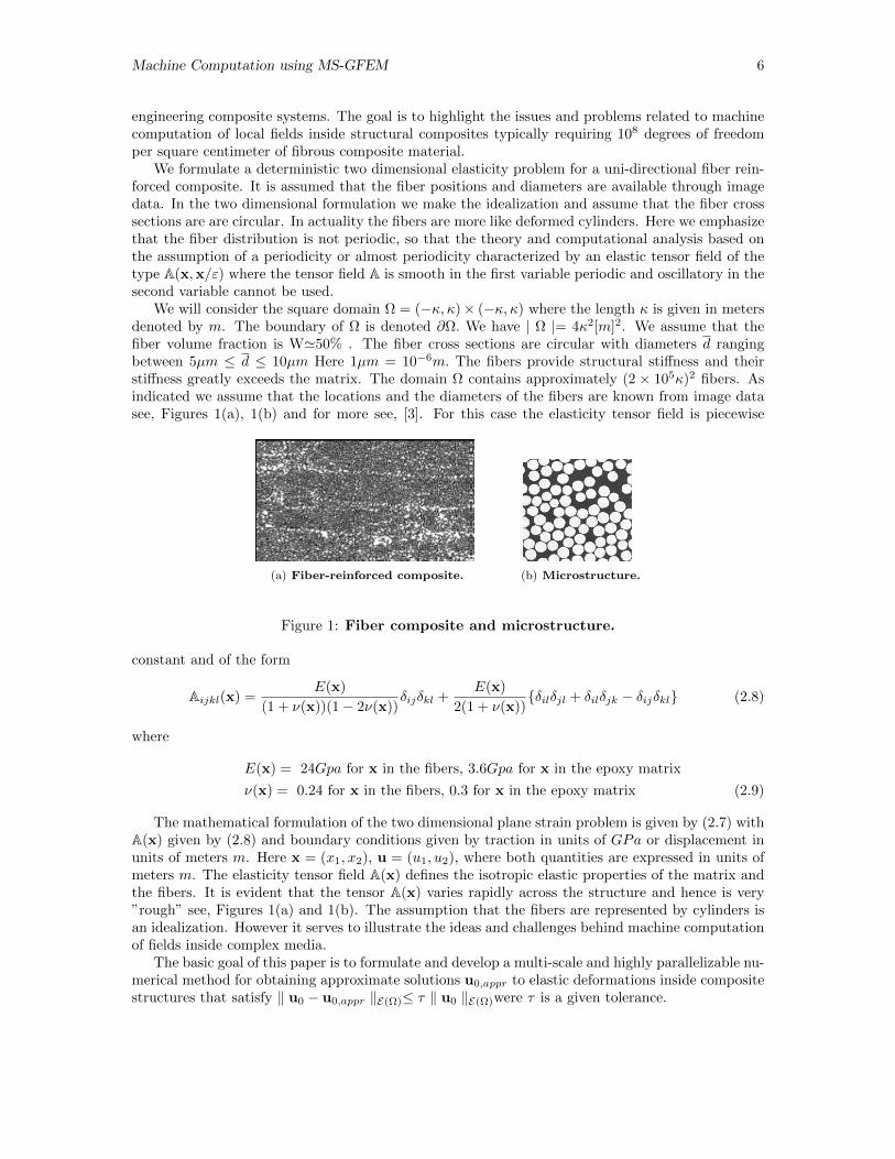
We will consider the square domain Ω = (−κ, κ)× (−κ, κ) where the length κ is given in metersdenoted by m. The boundary of Ω is denoted ∂Ω. We have | Ω |= 4κ2[m]2. We assume that thefiber volume fraction is W'50% . The fiber cross sections are circular with diameters d rangingbetween 5µm ≤ d ≤ 10µm Here 1µm = 10−6m. The fibers provide structural stiffness and theirstiffness greatly exceeds the matrix. The domain Ω contains approximately (2 × 105κ)2 fibers. Asindicated we assume that the locations and the diameters of the fibers are known from image datasee, Figures 1(a), 1(b) and for more see, [3]. For this case the elasticity tensor field is piecewise

(a) Fiber-reinforced composite. (b) Microstructure.

Figure 1: Fiber composite and microstructure.

constant and of the form

Aijkl(x) =E(x)

(1 + ν(x))(1− 2ν(x))δijδkl +

E(x)

2(1 + ν(x))δilδjl + δilδjk − δijδkl (2.8)

where

E(x) = 24Gpa for x in the fibers, 3.6Gpa for x in the epoxy matrix

ν(x) = 0.24 for x in the fibers, 0.3 for x in the epoxy matrix (2.9)

The mathematical formulation of the two dimensional plane strain problem is given by (2.7) withA(x) given by (2.8) and boundary conditions given by traction in units of GPa or displacement inunits of meters m. Here x = (x1, x2), u = (u1, u2), where both quantities are expressed in units ofmeters m. The elasticity tensor field A(x) defines the isotropic elastic properties of the matrix andthe fibers. It is evident that the tensor A(x) varies rapidly across the structure and hence is very”rough” see, Figures 1(a) and 1(b). The assumption that the fibers are represented by cylinders isan idealization. However it serves to illustrate the ideas and challenges behind machine computationof fields inside complex media.

The basic goal of this paper is to formulate and develop a multi-scale and highly parallelizable nu-merical method for obtaining approximate solutions u0,appr to elastic deformations inside compositestructures that satisfy ‖ u0 − u0,appr ‖E(Ω)≤ τ ‖ u0 ‖E(Ω)were τ is a given tolerance.


3 Generalized finite elements and multiscale formulation

For completeness we now review the basic theory of the GFEM method as it applies to the problemtreated here. For the proofs we refer to [4]. The elastic deformation u0 inside the composite is asolution of the problem u0 ∈ E(Ω),u0 = uΓ on Γ ⊂ ∂Ω,

B(u0,v) = F (v),∀v ∈ E(Ω),v = 0 on Γ (3.1)

Let ωjNj=1, j = 1, 2..N be a collection of open patches satisfying ωj ⊂ Ω and Ω = ∪Nj=1ωj and

assume that any x ∈Ω belongs at most to ς patches ωj . Let φjNj=1 be family of functions definedon Ω, having piecewise continuous derivatives, and satisfying the following properties

φj(x) = 0, for x ∈ Ω \ ωj , j = 1, 2, ..N, (3.2)

N∑j=1

φj(x) = 1,∀x ∈ Ω, (3.3)

maxx∈Ω

| φj(x) |≤C1, j = 1, 2, ..N (3.4)

maxx∈Ω

| ∇φj(x) |≤C2/diam(ωj), j = 1, 2, ..N (3.5)

where 0 ≤ C1, C2 < ∞ and diam(ωj) is diameter of ωj . It is evident that φj is a partitionof unity on Ω. To every ωj we associate on ωj an m(j) + 3−dimensional space Vj given by thespan of functions ξji = (1ξji,

2ξji) ∈ E(Ω), i = 1, 2, ...,m(j), together with the span of the basis,ξj,m(j)+1 = (1, 0), ξj,m(j)+2 = (0, 1), ξj,m(j)+3 = (−x2, x1) for the three dimensional space of rigidmotions in R2 denoted by R. Let

ξj =

m(j)+3∑i=1

bjiξji, bji ∈ R, i = 1, . . . ,m(j) + 3 (3.6)

Let S be the span of all functions of the form

ψ =

N∑j=1

φjξj , ξj ∈ Vj (3.7)

or equivalently S is given by the span

S = spanηji, i = 1, 1, 2, ...m(j) + 3, j = 1, 2, ...N. (3.8)

whereηji = φjξji ∈ E(Ω) (3.9)

The space Vj is called a local approximation space and the space S the finite element space. Nowwe have Theorem 3.1

Theorem 3.1. Suppose first that Γ = ∅, i.e, only boundary tractions on ∂Ω tractions are prescribed.

1. Every Vj contains the subspace of rigid body motions and ‖ v ‖L2(ωj)≤ C3diam (ωj) ‖ v ‖E(ωj)

for all v ∈ E(ωj) satisfying∫ωj

(v · r)dωj = 0 where r is a rigid body motion.

2. Let u ∈E(Ω) and for every j there is ξj ∈ Vj such that

‖ u− ξj ‖E(ωj)≤ εj . (3.10)


Then there exists ξj ∈ Vj such that for

ξ =

N∑j=0

φjξj (3.11)

we have

‖ u− ξ ‖E(Ω) ≤ C4(

N∑j=1

ε2j ) = C4ε (3.12)

with C4 = (2ς(C21 + C2

2C23 ))1/2. If Γ 6= ∅ and ωj ∩ Γ, then Vj is the hyperplane such that if ξ ∈Vj

then ξ = uΓ on ωj ∩ Γ

Now we are able to formulate the GFEM. Consider the boundary value problem (3.1) and assumefirst that Γ = ∅. Let u0 be the solution of the problem (3.1), i.e., u0 ∈ E(Ω) satisfies

B(u0,v) =F (v),∀v ∈E(Ω). (3.13)

and the solution is unique up to rigid body motion. Now the GFEM approximation u0,appr ∈ S,satisfies

B(u0,appr,v) = F (v),v ∈ S. (3.14)

and the solution is also unique up to rigid body motion. It immediately follows from theorem 3.1that

‖ u0 − u0,appr ‖E(Ω)≤ C4ε. (3.15)

If Γ 6= ∅, and ωj ∩ Γ 6= 0 we can assume that inequality (3.15) holds once the space Vj isappropriately modified.

4 Optimal local approximation spaces via spectral bases

In this section we introduce the optimal local bases. The basis functions appear as solutions ofa special kind of eigenvalue problem involving A harmonic functions. In fact it turns out that itis impossible to improve on their approximation properties; this is shown in Section 7 where anexponential upper bound on the local approximation error is developed.

Let ω ⊂ ω∗ ⊂ Ω ⊂ R2 be two concentric square domains inside the composite material introducedin Section 3. We choose an intermediate length scale H. We assume H is larger than the lengthscale of the fiber diameter and fiber spacing d but smaller than the dimensions of the domainΩ containing the composite. To fix ideas we write H = γd, where γ ∼ 1 × 102. Here we takeω = (−(1 + α)H/2, (1 + α)H/2)2, 0 < α < 1 and ω∗ = (−(1 + α)H, (1 + α)H)2. The energy innerproducts associated with these subsets are defined by

(u,v)E(ω∗) =

∫ω∗

Ae(u) : e(v) dx. (4.1)

(u,v)E(ω) =

∫ω

Ae(u) : e(v) dx. (4.2)

For any open subset S of the computational domain Ω we introduce the space of functions HA(S;R2)defined to be the functions in H1(S;R2) that are A-harmonic on S, i.e., v ∈ H1(S;R2) and

(v, ϕ)E(S) =

∫S

Ae(v) : e(ϕ) dx, ∀ϕ ∈ C∞0 (S;Rd). (4.3)

Since we work with the energy inner product we introduce the quotient space of HA(ω∗;R2) withrespect to rigid motions R denoted by HA(ω∗;R2)/R. We also introduce the subspace H0

A(ω∗;R2)


given by elements of HA(ω∗;R2) perpendicular to rigid motions with respect to the L2(ω∗;R2)inner product. Here we recall that HA(ω∗;R2)/R equipped with the energy norm is isometric toH0

A(ω∗;R2). We define the linear map T from HA(ω∗;R2)/R into HA(ω;R2)/R as the restrictionof u ∈ HA(ω∗;R2)/R to ω,, i.e., T u(x) = u(x) for x ∈ ω. The operator T is compact, thisfollows immediately from an application of the Caccioppoli inequality Lemma 7.6 together withthe Rellich Kondrachov embedding theorem on ω∗ see [7]. Let T ∗ be the adjoint mapping i.e.,(T ϕ,ψ)E(ω) = (ϕ, T ∗ψ)E(ω∗) for all ϕ ∈ HA(ω∗;R2)/R and ψ ∈ HA(ω;R2)/R and the operatorT ∗T is a compact operator mapping HA(ω∗;R2)/R into itself. The eigenvalue problem for the selfadjoint bounded compact operator is written

T ∗T ϕ = λϕ. (4.4)

The eigenfunction, eigenvalue pairs are denoted by ϕj and λj , j = 1, 2, . . .. With λj > 0 and theeigenvalues form a decreasing sequence λj ≥ λj+1.. The eigenvalues λj ≤ 1, j = 1, 2, .. are shown todecay exponentially i.e.,

λj ' e−jq

, (4.5)

where q = 13 − ε. For three dimensional problems q = 1

4 − ε, see Theorem 7.3 equation (7.8)and the discussion in Section 7. The eigenfunctions ϕj form a complete orthonormal system forHA(ω∗;R2)/R , i.e., (ϕi,ϕj)E(ω∗) = 0 for i 6= j, ‖ ϕj ‖E(ω∗)= 1. In addition they enjoy orthogonality

on ω, i.e., (ϕi, ϕj)E(ω) = 0 for i 6= j and

‖ ϕj‖E(ω) = λ1/2j ‖ ϕj ‖E(ω∗) . (4.6)

For ϕ ∈ HA(ω∗;R2)/R one has

ϕ =

∞∑j=1

cjϕj , with cj = (ϕ,ϕj)E(ω∗)

∞∑j=1

c2j =‖ ϕ‖2E(ω∗) and ‖ ϕ ‖2E(ω)=

∞∑j=1

c2jλj . (4.7)

From which we deduce the approximation property

‖ ϕ−m∑j=1

cjϕj ‖2E(ω)=

∞∑j=m+1

c2jλj ≤ λm+1 ‖ ϕ‖2E(ω∗). (4.8)

It now follows that any A harmonic function ϕ ∈HA(ω∗;R2)/R can be approximated over ω by them dimensional space V = spanϕj : j = 1, 2, . . . ,m with the error given by λm+1 ‖ ϕ‖E(ω∗).Moreover this choice of space V is optimal in the sense that no other m dimensional space can leadto a better approximation for all ϕ ∈ HA(ω∗;R2)/R. This is shown in Section 7. It is pointed outthat the optimal approximation space is not necessarily unique.

Presently the a priori knowledge of the higher regularity of the eigenfunctions ϕj for fibercomposites remains an open question. As of now it is not known if the eigenfunctions belong to theBesov space Hα(ω∗), for some α > 1. With this in mind we make the hypothesis.

Hypothesis 4.1. We consider the Besov space Bα2,∞(ω∗) denoted by Bα(ω∗) and suppose that thefollowing inequality holds

‖ ϕj ‖Bα(ω∗)≤ CH−1/2jβ ‖ ϕj‖E(ω∗), (4.9)

with α = 3/2 and β ≥ 1/2.


We assume α = 3/2 since the matrix A associated with the fiber reinforced composite in (2.3) ispiecewise constant see, Figure 1(b). Here we will also assume that the fibers are not touching.

Remark 4.2. Here the exponent β is not chosen. However because of the exponential approximationproperties the maximum number of spectral basis elements required for a prescribed approximationerror τ grows slowly, i.e., j ≤ [ln(τ−1)]d+1. This feature mollifies the influence of the exponent β.

As before d denotes the length scale associated with the fiber diameters and distance betweenfibers. We consider a uniform mesh of diameter h < d chosen to deliver an approximation with anaccuracy τ . For this mesh the best piecewise bilinear finite element approximation to ϕj is denotedby ϕ∗j,h and

‖ϕj − ϕ∗j,h‖E(ω∗) ≤ Ch1/2 ‖ ϕj ‖B3/2(ω∗) . (4.10)

Combing this estimate with the regularity hypothesis (4.9) delivers the desired estimate in terms ofthe energy ‖ ϕ‖E(ω∗) given by

‖ϕj − ϕ∗j,h‖E(ω∗) ≤ Ch1/2H−1/2jβ ‖ ϕ‖E(ω∗). (4.11)

Here we have addressed the approximation of A harmonic functions over local domains ω ⊂ ω∗.When the equilibrium equation (2.1) is inhomogeneous on ω∗ we can decompose the solution intou0 = u− χ+ χ, where χ belongs to H1

0 (ω∗;R2) and is the local particular solution of

−div(A(x)e(χ(x))) = f(x)

for x ∈ ω∗. Here the difference u0−χ belongs to HA(ω∗;R2) and can be approximated exponentiallywell using the spectral basis ϕjmj=1.

We now consider local domains ω that border the boundary ∂Ω. The configuration of ω and ω∗

for domains bordering the boundary is shown in Figure 2 see, section 7. Here ω ⊂ ω∗ and bothdomains have boundary components that coincide with ∂Ω. Spectral bases can be found for domainsω∗ bordering the boundary ∂Ω for which the solution u0 is A-harmonic and satisfies a homogeneoustraction or Dirichlet condition on ∂ω∗∪∂Ω. The spectral bases for domains bordering the boundaryalso satisfy (4.6), (4.7), (4.8), and the associated eigenvalues decay exponentially (4.5) see, Theorem7.5. When faced with non-homogeneous boundary conditions on ∂ω∗ ∪ ∂Ω, and body force f wesolve for the local particular solution η of

−div(A(x)e(η(x))) = f

for x ∈ ω∗ with non-homogeneous traction or Dirichlet boundary conditions on ∂ω∗ ∪ ∂Ω and η = 0on ∂ω∗∩Ω. For this case the difference u0−η is A-harmonic with homogeneous boundary conditionson ∂ω∗ ∪ ∂Ω and can be approximated exponentially well by the spectral basis.

5 Multiscale Spectral GFEM and error estimates

In this section we provide a-priori error estimates for the discrete approximation of the compositematerial problem introduced in Section 2. We start by assuming that the local spectral bases can becomputed with infinite accuracy. We apply this hypothesis and use the local spectral basis within theGFEM Galerkin scheme to provide the a-priori error estimate given by (5.3). In the second part ofthis section we introduce the discrete finite element approximation to the local spectral bases. Thisis used together with (5.3) to establish the a-priori error estimate for the GFEM implementationusing the discrete local approximation. This estimate is given by (5.12). This estimate allows us toassess the computational complexity of the multi-scale GFEM using optimal local bases provided inSection 6.

Recall that the domain containing composite material is given by Ω = (−κ, κ)2. We cover itwith a mesh defined by the nodal points zi,j = (xi, yj), xi = iH, yj = jH, with i, j = ±0, 1, 2, ...n,


and H = κ/(1 + α)(n+ 1/2) where 0 < α < 1 is chosen below. Let Qi,j be squares with center zi,jand side length µ(Qi,j) = H. We define ωi,j to be given by the square Qαi,j with center in zi,j and

side length µ(Qαi,j) = (1 + α)H, 0 < α < 1. Further let ω∗i,j = Ω ∩Qα∗i,j with α∗ = β(1 + α). Now wefix α = 1/4 and β = 2. For this choice the domains ω∗ij are squares of side length H∗ = 2.5H. It isevident that Ω = ∪i,jωi,j and the domains ωi,j overlap where the width of the overlap region is H/4.In what follows domains ωi,j bordering ∂Ω, (i.e., ωi,j ∩ ∂Ω 6= 0) are called boundary subdomainsand all others are referred to as interior subdomains. We now construct the partition of unity. LetQαij be the square of side length (1−α)H with center zij . Consider interior subdomains ωij and let

φi,j = 1 on Qαi,j , φi,j = 0 on Ω− ωi,j and be piecewise linear on ωi,j − Qαi,j . For boundary domains

ωi,j set φi,j = 1 over parts where ωi,j does not overlap any other ωk,l. The collection of functionsφi,j constitute a partition of unity i.e.,

∑i,j φ

i,j = 1 and can be employed within the GFEM see,Section 3.

On every interior domain ωij ⊂ ω∗i,j ⊂ Ω the functions ϕ(l)i,j l = 1, ...m(i, j) are elements of

the local spectral bases introduced in the previous section. Consider the span of the local basis

ϕ(l)i,j , l = 1, ....m(i, j) defined on ω∗i,j together with the three dimensional span of the basis for rigid

rotations in R2 and denote this m(i, j) + 3 dimensional space by Wm(i,j)i,j . If ω∗i,j is a boundary

subdomain and a non-homogenous boundary condition is prescribed on the boundary component

common to ∂ω∗i,j and ∂Ω, then the space Wm(i,j)i,j is augmented by ψpi,j where the function ψpi,j

is the A−harmonic function satisfying the non-homogeneous boundary condition and ψpij = 0 on

∂ω∗ij ∩ Ω. In addition if the right hand side is not zero the we augment the space Wm(i,j)i,j by

a function χijwhere χij is a particular solution on of ω∗ij with homogeneous Dirichlet boundary

data on ∂ω∗ij . For the two dimensional problem treated here we have N = (2n)2 subdomains ωijand the associated partition of unity

∑ij φij = 1. We set m = minijm(i, j) and for this explicit

application the multi-scale GFEM basis Wm is given by the span of all functions of the form

ϕ =∑

|i|≤1,|j|≤n

φijξij , ξij ∈Wm(i,j)i,j . (5.1)

We write this as Wm =∑i,j φijW

m(i,j)i,j and Wm ⊂ E(Ω). Let ϕp =

∑ij φijψ

pij be the sum of

local particular solutions and set ϕ =∑ij φijξij where ξij belong to the local spectral basis over

ωij . Then ϕp + ϕ ∈ Wm. Given a solution u0 of the boundary value problem (3.1) we consider itsrestriction to ωij . Note that u0 − (ϕp + ϕ) = (u0 − ϕp)− ξij on ωij and u0 − ϕp is A-harmonic onω∗ij and we recall the exponential approximation property of the local spectral bases described inthe previous section to see that we can construct a ϕ ∈Wm for which

‖u0 − (ϕp + ϕ)‖E(ωij) = ‖(u0 − ϕp)− ϕ‖E(ωij)

≤ C0e−(m(i,j)+1)q‖u0 − ϕp‖E(ω∗ij)

≤ C1e−(m+1)q‖u0‖E(ω∗ij)

. (5.2)

Now we apply Theorem 3.1 to discover that there is an approximation ϕ ∈Wm for which

‖ u0 − ϕ ‖2E(Ω)≤ C∑i,j

e−2(m(i,j)+1)q ‖ u0 ‖2E(ω∗i,j)

≤ C2e−2(m+1)q ‖ u0 ‖2E(Ω)= C2τ2 ‖ u0 ‖2E(Ω) (5.3)

Here we have set τ = e−(m+1)q , where q = 13 − ε. This is the a-priori estimate for the error assuming

a perfect computation of the local spectral bases. Here we view the local domains ωij as coarseelements of size H. In the estimate (5.3) we have assumed that the eigenvalue problem can besolved exactly.

With the estimate (5.3) in hand we now carry out the a-priori estimate assuming a finite elementapproximation of the spectral bases on ω∗ij . Let Tij,h be uniform mesh square of elements size h on


ωij which coincides with the boundary ∂ω∗ij and ∂ωij . The finite element space of bilinear elementson Tij,h is written Vij,h. Denote by HA,h(ω∗ij) the space of discrete A−harmonic functions on ω∗ij , i.e.,HA,h(ω∗ij) = v ∈Vij,h, B(v, z) =0,∀z ∈Vij,h, z = 0 on ∂ω∗ij. Now the finite element approximation

to the spectral problem is to find ϕ(l)ij,h ∈ HA,h(ω∗ij) and λ

(l)ij,h such that

(ϕ(l)ij,h, χ)E(ωij) = λ

(l)ij,h(ϕ

(l)ij,h, χ)E(ω∗ij)

,∀χ ∈ HA,h(ω∗ij). (5.4)

Based on the relation between the approximate eigenfunctions ϕ(l)ij,h and the best bilinear finite

element approximation of the exact eigenfunctions ϕ∗(l)ij,h see, [11], and using the Hypothesis 4.1 and

the associated inequalities 4.9 and (4.11) we have

‖ ϕ(l)ij − ϕ

(l)ijh ‖E(ω∗ij)

≤ C1(l) ‖ ϕ(l)ij − ϕ

∗(l)ij,h ‖E(ω∗ij)

(5.5)

and

| λ(l)ij − λ

(l)ijh |≤ C2(l) ‖ ϕ(l)

ij − ϕ∗(l)ij ‖

2E(ω∗ij)

. (5.6)

Unfortunately the dependence of the constants C1and C2 on l is not available. Hence we make the

Hypothesis 5.1. We have that the positive constants C1 and C2 are bounded above by Clα

Applying hypotheses 4.1, 5.1 and (4.11) we get

‖ ϕ(l)ij − ϕ

(l)ijh ‖E(ω∗ij)

≤ CH−1/2lα+βh1/2 ‖ ϕ(l)ij ‖E(ω∗ij)

(5.7)

and

| λ(l)ij − λ

(l)ijh |

1/2≤ CH−1/2h1/2lα+β ‖ ϕ(l)ij ‖E(ω∗ij)

(5.8)

Recalling (5.2) we see that u0 − ϕp ∈ HA(ω∗i,j ;R2) can be approximated by local spectral bases so

that for m ∼ [ln(τ−1)]3, ‖ u0 − (ϕp +∑ml=1 c

(l)ij ϕ

(l)ij ) ‖E(ωij)≤ Cτ ‖ u0 −ϕp ‖E(ω∗ij)

. Applying this we

see that

‖ (u0 − ϕp)−m∑l=1

c(l)ij ϕ

(l)ij,h ‖E(ωij)

≤‖ (u0 − ϕp)−m∑l=1

c(l)i,jϕ

(l)ij ‖E(ωij) +

m∑l=1

| c(l)ij |‖ ϕ(l)ij − ϕ

(l)ij,h ‖E(ω∗ij)

≤ Cτ ‖ (u0 − ϕp) ‖E(ω∗ij)+CH−1/2h1/2

m∑l=1

| c(l)ij | lα+β

≤ Cτ ‖ (u0 − ϕp) ‖E(ω∗ij)+CH−1/2h1/2mα+β(

∞∑l=1

c(l)2ij )1/2

≤ C(τ +H−1/2h1/2(log τ−1)3(α+β)) ‖ (u0 − ϕp) ‖E(ω∗ij). (5.9)

It now follows that the solution u0 can be approximated on ωij by the finite element approximationof the local spectral basis and local particular solution denoted by ϕph

‖ u0 − (ϕph +

m∑l=1

c(l)ij ϕ

(l)ij,h) ‖E(ωij)

≤ C(τ +H−1/2h1/2(1 + [log τ−1]3(α+β))) ‖ u0 ‖E(ω∗ij), (5.10)

where C is independent of τ , h, H and i, j. Hence given τ we can select h to get

infc(l)

‖ u0 − (ϕph +∑

c(l)ϕ(l)ij,h) ‖E(ωij)≤ Cτ ‖ u0 ‖E(ω∗ij)

. (5.11)


Let Wm(i,j)i,j,h be the span of the functions vk, k = 1, 2, 3 and ϕ

(l)i,j,h, l = 0...m(i, j) augmented with the

finite element approximations to the local particular solutions and take W(m)h =

∑i,j ⊕φijW

(m(i,j))i,j,h .

It is now evident that there is an approximation u0,appr ∈W (m)h for which

‖ u0 − u0,appr ‖E(Ω)≤ Cτ ‖ u0 ‖E(Ω) . (5.12)

which is the fully discrete analog of (5.3).We conclude with the following remarks

Remark 5.2. In the estimate (5.10) above we had chosen h ∼ τ2 to recover (5.11). This is becausewe used a uniform mesh and first order finite elements when the eigenfunctions participating in thespectral basis had discontinuous gradient across material interfaces.

Remark 5.3. The eigenfunctions are piecewise analytic inside ω∗ and have singular behavior at thepoints of ∂ω∗ where it is intersected by the fiber boundaries. The theory of the eigenvalue problemis very general. It requires only that the distance of the boundaries ∂ω∗ and ∂ω is of the same orderas the diameter of ω. Hence we can create a ”wiggly” ω∗∗ when the boundary ∂ω∗∗ is separatedfrom the fibers by a distance on the order of the fiber diameter and is near by to the boundary ofω∗. In this scenario the eigenfunctions belong to the ”broken” Sobolev space of arbitrary order. Herea broken Sobolev space is the space which belongs to H1(ω∗∗) and also to Hk within the fibers andexterior to the fibers. For this case if we use the curved elements or GFEM/XFEM we can gethigh order rate of convergence i.e N ∼ τ−2/(k−1)where N is the number of degrees of freedom. Notethat the exponential decay of the eigenvalues λ(l) leads to very mild assumptions about the regularityof the eigenfunctions as put forth in Hypothesis 4.1.

6 Computational complexity for MS-GFEM

In this section the aim is to assess the computational complexity and estimate the cost of the proposedMS-GFEM method for solving the composite material problem. The assessment is qualitative in thatit is expressed in terms of constants which are theoretically known but are not necessarily optimal.The computation consists of the following parts: 1) Construction of the uniform mesh of size H onΩ over which the subdomains ωi,j and ω∗i.j are defined. 2) Construction of the spectrally defined

shape functions ϕlij,h on each subdomain ωi,j . 3) Construction of the stiffness matrix and the righthand side of the MS-GFEM problem. 4) Solving the system of equations of MS-GFEM. Components1,2,3 can be carried out independently over each subdomain ωij and are used to construct the linearsystem in part 4. To give perspective on a large parallel machine each subdomain computation canbe carried out on a separate core independently of the other cores. The linear system to be solvedin part 4 is much smaller in size when compared to the full FE discretization of the problem andcan be solved using parallel algorithms.

1. Construction of the coarse mesh of size H and the associated domains ωij,ω∗ij . This step is

straight forward and inexpensive. In what follows we will identify the considerations leadingto an optimal choice of H that minimizes the time of computation.

2. The construction of the local shape functions ϕlij,h on each ωij. involves five components.

(a) On ω∗ij we construct the uniform mesh of squares of size h so that the boundaries ∂ωijand∂ω∗ij coincide with the mesh. The size h is chosen according to the tolerance τ as discussedin the previous section.

(b) Construction of the stiffness matrix for the problem on ω∗ij . From the previous sectionthese domains are squares of sidelength β(1 + α)H = H∗. Because the tensor A isdiscontinuous across material interfaces we point out that adaptive integration schemesneed to be used. Because of the sparsity of the stiffness matrix the number of operationsrequired for assembly is O(H∗/h).


(c) Construction of the space HA,h(ω∗ij) of discrete A-harmonic functions on ω∗ij . Motivatedby the numerical experiments of [55] we construct a 2N dimensional space of discretefinite element A-harmonic functions spanned by the functions wlij,h on ω∗ij . Thesefunctions are defined to be discretely A-harmonic with traces on ∂ω∗ij corresponding tothe basis of harmonic polynomials of degree ≤ N . The choice of N is determined at the

time of computation and is conditioned on the eigenvalue λ(2N+1)ij,h of the discrete spectral

problem (5.4). Here we choose N such that λ(2N+1)ij,h ≤ τ. We then select the dimension

of the discrete approximation space to be m such that λ2m+1ij,h ≤ τ . For the purposes of

estimation we start with N = 100. The functions wlij,h can be computed iteratively usingconjugate gradient methods and preconditioning or by Gaussian elimination. Here we willassume that each of the discrete functions wlij,h is obtained iteratively using q iterations

so that O(2Nq(H/h)2) operations are required to construct a discrete 2N dimensionalharmonic subspace of HA,h(ω∗ij). Alternatively using Gaussian elimination would require

O((2NH/h)3) operations to create the 2N dimensional subspace.

(d) Construction of the eigenvalue problem leading to the local shape functions ϕlij,h. Thelocal discrete eigenvalue problem (5.4) delivers the matrix eigenvalue problem of the formλPx = Qx. Here Pkl = (wkij,h, w

lij,h)ω∗ij , and noting that the local basis functions wkih,h

and wlij,h are A-harmonic shows (on integrating by parts) that computing one element of

P requires O(H/h) operations. Hence O(4N2H/h) operations are required to assembleP . The same estimate applies to the number of operations needed to assemble Q.

(e) Solution of the eigenvalue problem requires O((2N)3) operations.

Summarizing we see that to obtain the approximation space spanned by 2N local shapefunctions given by the spectral basis ϕlij2Nl=1 the cost is dominated by the number of op-

erations required to construct the finite dimensional discrete subspace spanned by wlij,h.This cost is O(2Nq(H/h)2) operations using the iterative approach for finding each wlij,hand O((2NH/h)3) operations using Gaussian elimination. Assuming that q = N we needO(2N2(H/h)2) respectively O(8N3H3/h3) operations for determining ϕlij2Nl=1.

3. Construction of the MS-GFEM stiffness matrix and the right hand side,

(a) Construction of the MS-GFEM stiffness matrix. The MS-GFEM stiffness matrix is ablock diagonal matrix associated with the 9 point stencil. Here each block is an m ×mmatrix. The construction of the block matrices is carried out locally and can be donein parallel. Here each stencil requires O(m2(H/h)2) operations to assemble and we have(κ/H)2 stencils.

(b) Construction of the right hand side. For problems driven by body forces one has a pre-scribed right hand side function f . For this case we compute (κ/H)2 particular solutionswij . Here we need O(H/h)2) operations to compute each local particular solution wij .The construction is carried out locally and independently over each ω∗ij and can be donein parallel.

4. Solution of the MS-GFEM system. For problems with multiple right hand sides we can in-vert the matrix using elimination to recover the discrete solution operator. This requiresO((κ/H)3m3) operations. The solution procedure is parallelizable but requires communica-tion between cores. Alternatively for single right hand sides one can proceed using iterativemethods.

We now address the computational complexity for the MS-GFEM and estimate the machine timerequired for computation. To begin we consider implementation first on a single processor and thenon a parallel machine with p processors. Here we ignore other issues such as the cost of fetches todisk when using a single processor.


1. Single processor implementation. Carrying out steps 1 through 3 requires O(N2H2/h2) op-erations for each of the (κ/H) 2 subdomains ωij for a total of O(κ2N2/h2) operations. If weapply elimination to construct the local subspaces then O(N3H3/h3) operations are requiredover each subdomain and we have a total of O(κ2N3H/h3) operations. Thus to carry outsteps 1 through 3 on a single processor requires O(κ2N2/h2) resp O(κ2N3H/h3) operations.Step 4 requires O(m3κ3/H3) operations. It follows that single processor implementation ofMS-GFEM requires

O(κ2N2/h2) +O(κ3m3/H3) and (6.1)

O(κ2N3H/h3) +O(m3κ3/H3) (6.2)

operations respectively. Fixing h,N,m in (6.1) and choosing H so that both terms are ofthe same order we have H ∼ O(κ1/3mh2/3/N2/3) and the total number of operations isO(κ2N2/h2). Similarly fixing h in (6.2) and choosing H so that both terms are of the sameorder gives resp H = m3/4κ1/4h3/4/N3/4and the total number of operations isO(N9/4m1/4κ9/4/h9/4).

Equation (6.1) shows that the local approximation spaces together with the inversion of theGFEM stiffness matrix delivers the complete inverse operator for the discrete problem with thesame number O(N2κ2/h2) of operations.

2. Now we consider a parallel implementation with p processors and provide an estimate forthe time necessary to perform the computation. Here the work is measured in floating pointoperations per second F and the total time is F × Operations. Here the time to executesteps one through three drops by a factor of 1

p . Step four using a direct solver within a parallel

implementation will roughly require FO(κ3m3/H3)/p+D(lg p)m(κ/H)+E(mκ/H)2p−1/2 sec .

Here D ∼ 10−6 and E ∼ 10−9 and the last two terms relate to the latency inherent in thedirect solver.

We emphasize that the implementation of MS-GFEM delivers the discrete solution operator usingthe same order of operations as the number of fibers inside the computational domain. This im-plementation is optimal in that the number of operations for solution is of the same order as theinput data for the problem. It is important to point out that the MS-GFEM matrix is of orderm2κ2/H2, where m = lnd+1( 1

τ ) where τ is the prescribed tolerance for the approximation errorhence the memory required to store the MS-GFEM inverse matrix can be controlled and can be oforder far less than the number of fibers contained within the computational domain.

We close this section with a discussion on local memory allocation and problem size. Here weexecute steps 1 through 3 of the MS-GFEM computation over a single patch ω∗ij on one processor.

Standard processors and associated cash memory can handle problems with (H/h)2 ≤ 106 degreesof freedom. For this scenario the time for the local computation will be on the order of one second.Now suppose that h = τ2 then we can choose H = 103τ2 and for τ = 10−2 we have H ∼ 10−1.Setting κ = 1 we have p = 102 processors and the size of the MS-GFEM inverse matrix is seen to beon the order of 105. Assuming that the number of fibers is proportional to 1

h2 we have 108 fibers inthe computational domain. Thus the MS-GFEM inverse matrix is three orders of magnitude smallerthan the number of fibers inside the computational domain.

7 Optimal Local Approximation Spaces

In this section we introduce and develop optimal local approximation spaces for use in the multi-scalescheme. These spaces are distinguished by their exponential approximation properties. Given thesolution u0 to the global problem and a prescribed tolerance τ we seek to find a local approximationon the patch ωj . In this section we show that it is possible to find a local approximation w fromthe optimal local space Ψj of dimension (ln τ−1)d+1, d = 2, 3 for which the error satisfies

‖u0 −w‖E(ωj) ≤ τ. (7.1)


In what follows we will establish the optimal local approximation properties in the general con-text of heterogeneous media for two and three dimensional elasticity problems characterized bymeasurable elasticity tensors A(x) satisfying the coercivity and boundedness conditions (2.2). Wewill also develop approximation properties for local domains that border the boundary of Ω. Herewe will establish exponential approximation results when Ω has reentrant corners and for generalLipschitz domains. We begin by identifying optimal local approximation spaces for interior domains.

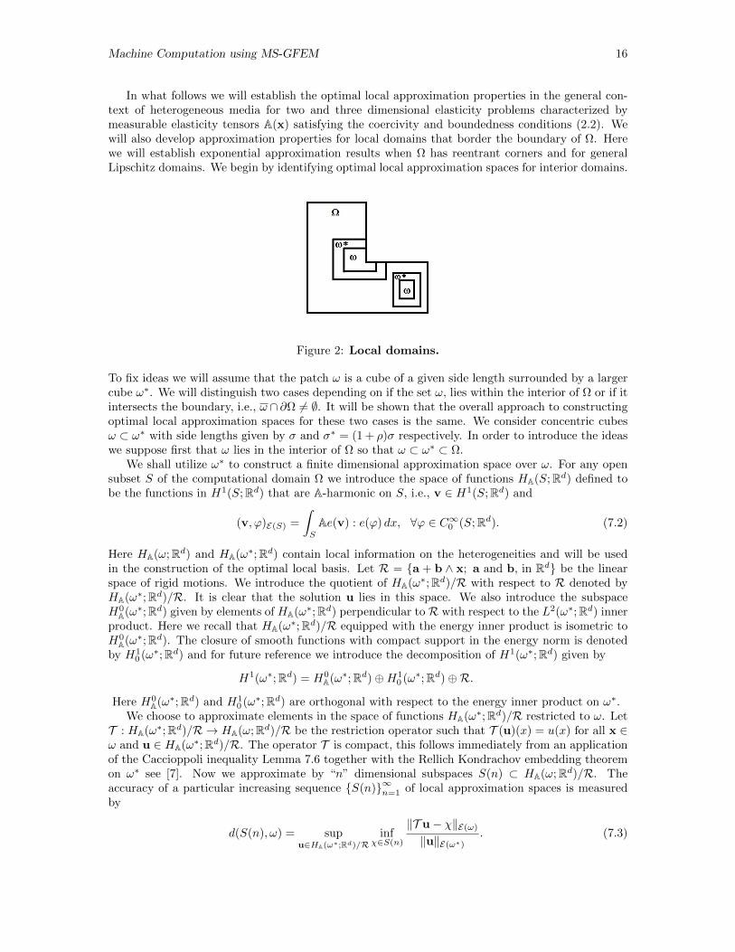
Figure 2: Local domains.

To fix ideas we will assume that the patch ω is a cube of a given side length surrounded by a largercube ω∗. We will distinguish two cases depending on if the set ω, lies within the interior of Ω or if itintersects the boundary, i.e., ω ∩ ∂Ω 6= ∅. It will be shown that the overall approach to constructingoptimal local approximation spaces for these two cases is the same. We consider concentric cubesω ⊂ ω∗ with side lengths given by σ and σ∗ = (1 + ρ)σ respectively. In order to introduce the ideaswe suppose first that ω lies in the interior of Ω so that ω ⊂ ω∗ ⊂ Ω.

We shall utilize ω∗ to construct a finite dimensional approximation space over ω. For any opensubset S of the computational domain Ω we introduce the space of functions HA(S;Rd) defined tobe the functions in H1(S;Rd) that are A-harmonic on S, i.e., v ∈ H1(S;Rd) and

(v, ϕ)E(S) =

∫S

Ae(v) : e(ϕ) dx, ∀ϕ ∈ C∞0 (S;Rd). (7.2)

Here HA(ω;Rd) and HA(ω∗;Rd) contain local information on the heterogeneities and will be usedin the construction of the optimal local basis. Let R = a + b ∧ x; a and b, in Rd be the linearspace of rigid motions. We introduce the quotient of HA(ω∗;Rd)/R with respect to R denoted byHA(ω∗;Rd)/R. It is clear that the solution u lies in this space. We also introduce the subspaceH0

A(ω∗;Rd) given by elements of HA(ω∗;Rd) perpendicular to R with respect to the L2(ω∗;Rd) innerproduct. Here we recall that HA(ω∗;Rd)/R equipped with the energy inner product is isometric toH0

A(ω∗;Rd). The closure of smooth functions with compact support in the energy norm is denotedby H1

0 (ω∗;Rd) and for future reference we introduce the decomposition of H1(ω∗;Rd) given by

H1(ω∗;Rd) = H0A(ω∗;Rd)⊕H1

0 (ω∗;Rd)⊕R.

Here H0A(ω∗;Rd) and H1

0 (ω∗;Rd) are orthogonal with respect to the energy inner product on ω∗.We choose to approximate elements in the space of functions HA(ω∗;Rd)/R restricted to ω. Let

T : HA(ω∗;Rd)/R → HA(ω;Rd)/R be the restriction operator such that T (u)(x) = u(x) for all x ∈ω and u ∈ HA(ω∗;Rd)/R. The operator T is compact, this follows immediately from an applicationof the Caccioppoli inequality Lemma 7.6 together with the Rellich Kondrachov embedding theoremon ω∗ see [7]. Now we approximate by “n” dimensional subspaces S(n) ⊂ HA(ω;Rd)/R. Theaccuracy of a particular increasing sequence S(n)∞n=1 of local approximation spaces is measuredby

d(S(n), ω) = supu∈HA(ω∗;Rd)/R

infχ∈S(n)

‖T u− χ‖E(ω)

‖u‖E(ω∗). (7.3)


A sequence of approximation spaces S(n) is said to be optimal if it has an accuracy d(S(n), ω) thatsatisfies d(S(n), ω) ≤ d(S(n), ω), n = 1, 2, . . ., when compared to any other sequence of approxi-mation spaces S(n). The problem of finding the family of optimal local approximation spaces isformulated as follows. Let

dn(ω, ω∗) = infS(n)

supu∈HA(ω∗;Rd)/R

infχ∈S(n)


‖u‖E(ω∗). (7.4)

Then the optimal family of approximation spaces Ψn(ω)∞n=1 satisfy

dn(ω, ω∗) = supu∈HA(ω∗;Rd)/R

infχ∈Ψn(ω)


‖u‖E(ω∗). (7.5)

The quantity dn(ω, ω∗) is known as the Kolomogorov n-width of the compact operator T , see [45].The optimal local approximation space Ψn(ω) for GFEM follows from general considerations. Weintroduce the adjoint operator T ∗ : HA(ω;Rd)/R → HA(ω∗;Rd)/R and the operator T ∗T is acompact, self adjoint, non-negative operator mapping HA(ω∗;Rd)/R into itself. We denote theeigenfunctions and eigenvalues of the problem

T ∗T u = λu (7.6)

by ϕi and λi and the optimal subspace Ψn is given by the following theorem.

Theorem 7.1. The optimal approximation space is given by Ψn(ω) = spanψ1, . . . , ψn, whereψi = T ϕi and dn(ω, ω∗) =

√λn+1.

For the case considered here the definitions of T and T ∗ show that the optimal subspace andeigenvalues are given by the following explicit eigenvalue problem.

Theorem 7.2. The optimal approximation space is given by Ψn(ω) = spanψ1, . . . , ψn whereψi = T ϕi and ϕi and λi are the first n eigenfunctions and eigenvalues that satisfy

(ϕi, δ)E(ω) = λi(ϕi, δ)E(ω∗), ∀δ ∈ HA(ω∗;Rd)/R. (7.7)

The next theorem provides an upper bound on the rate of convergence for the optimal localapproximation.

Theorem 7.3. Exponential convergence for interior approximations.For ε > 0 there is an Nε > 0 such that for all n > Nε

dn(ω, ω∗) ≤ e−n( 1

1+d−ε)

. (7.8)

Theorem 7.3 (proven below) shows that the asymptotic convergence rate associated with the optimalapproximation space is nearly exponential for the general class of L∞(Ω) coefficients satisfying thecoercivity and boundedness conditions (2.2).

We now present optimal local approximation spaces for domains bordering the boundary of Ω.These results hold for domains Ω of general shape including bounded Lipschitz regions. The essentialassumption is that the Rellich Kondrachov embedding theorem holds in Ω. To fix ideas we considerthe L shaped domain Ω with a reentrant corner and introduce optimal local approximation spacesfor domains that intersect the boundary ∂Ω. To illustrate the method consider concentric L shapedsubdomains ω ⊂ ω∗ of Ω containing the reentrant corner. See Figure 2. The arguments presentedhere naturally apply to other choices of ω and ω∗ that touch the boundary. The outer domain is


denoted by ω∗ and the concentric inner domain is denoted by ω. The side lengths of ω ⊂ ω∗ ⊂ σare given by σ and σ∗ = (1 + ρ)σ respectively.

Given a function u ∈ HA(Ω;Rd), d = 2, 3, the goal is to provide an approximation to u in ω.To this end we form a local particular solution up given by the A-harmonic function that satisfiesAe(up)n = g on ∂ω∗ ∩ ∂Ω and up = 0 on ∂ω∗ ∩ Ω. Writing u = up + u0 we see that Ae(u0)n = 0on ∂ω∗ ∩ ∂Ω and u0 = u on ∂ω∗ ∩ Ω. The objective of this section is to find the optimal family oflocal approximation spaces that give the best approximation to u0 = u−up in the energy norm overthe set ω. We introduce the space of functions HA,0(ω∗;Rd) given by all functions v ∈ H1(ω∗,Rd)that are A-harmonic on ω∗ and for which ∂νv ≡ Ae(v)n = 0 on ∂ω∗ ∩ ∂Ω.The analogous space offunctions defined on ω is denoted HA,0(ω;Rd). Since we approximate functions with respect to theenergy norm we introduce the quotient space of HA,0(ω∗;Rd) to the subspace of rigid translationsR denoted by HA,0(ω∗;Rd)/R. Now we introduce T : HA,0(ω∗;Rd)/R → HA,0(ω;Rd)/R givenby the restriction operator defined by T (u)(x) = u(x) for all x ∈ ω and u ∈ HA,0(ω∗;Rd)/R.The operator T is compact. As before this follows immediately from an application of a suitableCaccioppoli inequality (Lemma 7.6) together with the Rellich Kondrachov embedding theorem onω∗. Let S(n) be any finite dimensional subspace of HA,0(ω;Rd)/R and the problem of finding thefamily of optimal local approximation spaces is formulated in terms of the n-width of T . Let

dn(ω, ω∗) = infS(n)

supu∈HA,0(ω∗;Rd)/R

infχ∈S(n)


‖u‖E(ω∗∩Ω). (7.9)

Proceeding as before we introduce the adjoint operator T ∗ : HA(ω;Rd)/R → HA(ω∗)/R and theoperator T ∗T is a compact operator mapping HA,0(ω∗)/R into itself. The optimal approximatingspaces are described in the following theorem.

Theorem 7.4. The optimal approximation space is given by Ψn(ω) = spanψ1, . . . , ψn whereψi = T ϕi and ϕi ∈ HA,0(ω∗;Rd)/R and λi are the first n eigenfunctions and eigenvalues thatsatisfy

(ϕi, δ)E(ω) = λi(ϕi, δ)E(ω∗∩Ω), ∀δ ∈ HA,0(ω∗;Rd)/R, (7.10)

and dn(ω, ω∗) =√λn+1.

The next theorem provides an upper bound on the rate of convergence for the optimal localboundary approximation.

Theorem 7.5. Exponential convergence at the boundary.For ε > 0 there is an Nε > 0 such that for all n > Nε

dn(ω, ω∗) ≤ e−n( 1d+1−ε)

. (7.11)

Theorem 7.5 shows that the asymptotic convergence rate associated with the optimal boundaryapproximation space is nearly exponential for the general class of L∞(ω∗) coefficients A(x) satisfyingthe coercivity and boundedness conditions (2.2).

We provide a proof of exponential decay for interior subdomains noting that the proof for bound-ary domains proceeds along similar lines. The construction of the local approximation space is doneiteratively. We introduce the the first n eigenfunctions vi ∈ H1(ω∗;Rd), orthogonal to R, in theL2(ω∗;Rd) inner product, for the the eigenvalue problem

(vi,w)E(ω∗) = λi

∫ω∗

vi ·w dx, ∀ w ∈ H1(ω∗;Rd),

i = 1, . . . , n. The subspace spanned by these functions is denoted by Sn(ω∗). We introduce the spanof A harmonic functions given by

Wn(ω∗) = spanwi ∈ HA(ω∗;Rd) : wi = vi, on ∂ω∗, i = 1, . . . n. (7.12)


The orthogonal projection from H1(ω∗;Rd) onto H0A(ω∗;Rd) is denoted by PA. and one readily

checks that Wn(ω∗) = PASn(ω∗).We define the family of approximation spaces Fn(ω, ω∗) given by the restriction of the elements

of Wn(ω∗) to ω. In what follows we first show that Fn(ω, ω∗) is a family of local approximationspaces with a rate of convergence on the order of n−1/d, d = 2, 3. To show this we introduce asuitable version of the Caccioppoli inequality that bounds functions in the energy norm over anymeasurable subset O ⊂ ω∗ for which dist(∂O, ∂ω∗) > δ > 0 in terms of the L2 norm over ω∗.

Lemma 7.6. (Caccioppoli inequality) Let u be A-harmonic in ω∗ and belong to L2(ω∗;Rd) ∩H1loc(ω

∗;Rd). Then

‖ u ‖E(O)≤ (2(β)1/2/δ) ‖ u ‖L2(ω∗;Rd) . (7.13)

where β is defined in (2.2).

The proof of the Lemma follows that given in [7].Next we introduce the approximation theorem associated with the space Wn(ω∗) given by

Lemma 7.7. Let u ∈ H0A(ω∗;Rd) then there exists a vu ∈Wn(ω∗) such that

‖u− vu‖L2(ω∗;Rd) = infv∈Wn(ω∗)

‖ u− v ‖L2(ω∗;Rd)≤ Cnσ∗θnα−1/2 ‖ u ‖E(ω∗) d = 2, 3, (7.14)

where σ∗ is the side length of the cube ω∗, α is given by (2.2) Cn = n−1/d(1 + o(1)), d = 2, 3. Ford = 2, θ2 =

√2/(3π) and for d = 3, θ3 = [(1 + 4

√2)/(6π2)]1/3.

Proof. The lemma follows immediately from an upper bound on the quotient

T = supu∈∈H0

A(ω∗;Rd)

infw∈Wn(ω∗)

‖u−w‖L2(ω∗;Rd)

‖u‖E(ω∗). (7.15)

Fix u ∈ H0A(ω∗;Rd) and denote the projection of u onto Wn(ω∗) with respect to the energy norm

‖ · ‖E(ω∗) by PEu. Choosing w = PEu and noting that ‖(I−PE)u‖E(ω∗) ≤ ‖u‖E(ω∗) gives the upperbound

T ≤ supu∈H0

A(ω∗;Rd)

‖(I − PE)u‖L2(ω∗;R2)

‖(I − PE)u‖E(ω∗)= sup

u∈H0A(ω∗;Rd)⊥Wn(ω∗)

‖u‖L2(ω∗;R2)

‖u‖E(ω∗). (7.16)

Since Wn(ω∗) = PASn(ω∗) it follows that

u ∈ H0A(ω∗;Rd) ⊥ PASn(ω∗) = u ∈ H0

A(ω∗;Rd) ⊥ Sn(ω∗),u ∈ H0

A(ω∗;Rd) ⊥ Sn(ω∗) ⊂ u ∈ H1(ω∗;Rd)2 ⊥L2 (Sn(ω∗)⊕R), (7.17)

where ⊥L2 in the second line of (7.17) denotes orthogonality with respect to the L2(ω∗;Rd) innerproduct. Hence

T ≤ supu∈H0

A(ω∗;Rd)⊥Sn(ω∗)

‖u‖L2(ω∗;Rd)

‖u‖E(ω∗)≤ sup

u∈H1(ω∗;Rd)2⊥L2 (Sn(ω∗)⊕R)

‖u‖L2(ω∗)

‖u‖E(ω∗)=

1√µn+1

, (7.18)

where µn+1 is the largest eigenvalue associated with Sn+1(ω∗). One has the elementary lower boundµn+1 ≥ ανn+1 where νn+1 is the largest corresponding eigenvalue for

∫ω∗e(vn+1) : e(w) dx =

νn+1

∫ω∗

vn+1 ·w dx, ∀w ∈ H1(ω∗;Rd). Here we can appeal to the generalization of Weyl’s theorem

for elastic problems [17] and νn+1 = 4π8(σ∗)2/3 (n + 1)(1 + o(1)), for d = 2 and νn+1 = [6π2/(1 +

4√

2)(σ∗)3/]1/3(n + 1)2/3(1 + o(1)) for d = 3. The required upper bound on T now follows andthe theorem is proved. Now we apply Lemma 7.6 together with Lemma 7.7 to obtain the followingconvergence rate associated with the family of approximation spaces Fn(ω, ω∗) given by


Theorem 7.8. Let u ∈ HA(ω∗;Rd)/R then there exists an approximation vu ∈ Fn(ω, ω∗) for which

‖ u− vu ‖E(ω) = infv∈Fn(ω,ω∗)

‖ u− v ‖E(ω)≤ I(ω, ω∗)Cn ‖ u ‖E(ω∗) (7.19)

where

I(ω, ω∗) = 4 θd1 + ρ

ρ(β/α)1/2 and Cn = n−1/d(1 + o(1)), d = 2, 3. (7.20)

Proof of Theorem 7.3. Next we proceed iteratively to construct a family of local approximationspaces with a rate of convergence that is nearly exponential. For any pair of two concentric cubesQ ⊂ Q∗ we define Fn(Q,Q∗) to be the space given by the restriction of Wn(Q∗) on Q. We supposethat ω∗ is of side length σ∗. Let N > 1 be an integer and we suppose that ω is of side length σ andσ∗ = σ(1 + ρ). Choose ωj , j = 1, 2, ...N to be the nested family of concentric cubes with side lengthσ(1 + ρ(N + 1− j)/N) for which ω = ωN+1 ⊂ ωN ⊂ ωN−1 ⊂ · · · ⊂ ω1 = ω∗. We introduce the localspaces, Fn(ω, ωN ), Fn(ω, ωN−1),...,Fn(ω, ω1). Put m = N × n and we define the approximationspace given by

T (m,ω, ω∗) = Fn(ω, ω1)⊕ · · · ⊕ Fn(ω, ωN ). (7.21)

Theorem 7.9. Let u ∈ HA(ω∗)/R and N be an integer such that 1 ≤ N ≤ nγ , with 0 < γ < 1/d.Then there exists zu ∈ T (m,ω, ω∗) such that

‖ u− zu ‖E(ω)≤ ςN ‖ u ‖E(ω∗) (7.22)

and ς = 4 θd1+ρρ N(β/α)1/2Cn, d = 2, 3.

Theorem 7.9 and the associated exponential decay given by Theorem 7.3 now follow from identicalarguments to those presented in [7]. The proof of Theorem 7.5 (exponential convergence for boundarydomains) proceeds along the same lines as the proof of Theorem 7.3 given above. Here one appliesthe elastic analog of Lemma 3.4 of [7], together with the version of the Caccioppoli inequality forboundary domains developed in [8] and the asymptotic decay result of [17].

8 Summary and perspective

Recent developments in aerospace and infrastructure are driving the need for new numerical methodsfor the recovery of local fields inside of large systems composed of heterogeneous structures. Severaldifferent approaches have been developed to address these problems as well as for complex multiscaleproblems in geology and biology. Even though it is possible to directly apply FEM methods to theseproblems the primary challenge facing a direct approach is that the linear system will be extremelylarge typically with degrees of freedom on the order 109 and higher. This requires methods whichare well suited to massively parallel computation. For heterogeneous media with high contrast andmillions of interfaces between component materials the use of multigrid methods is problematicbecause of the high contrast and non-uniform meshes etc. The use of iterative methods requiresuitable preconditioners adapted to the problem at hand. Gaussian elimination methods based onH-matrices [14] are not well parallelizable for three dimensional problems. There are also issues withthe control of accuracy when using nonuniform meshes and higher order elements.

The implementation of the MS-GFEM method proposed here delivers the discrete solution op-erator using the same order of operations as the number of fibers inside the computational domain.This implementation is optimal in that the number of operations for solution is of the same orderas the input data for the problem. The size of the MS-GFEM matrix used to represent the discreteinverse operator is controlled by the scale of the coarse grid and the convergence rate of the spectralbasis and can be of order far less than the number of fibers. This strategy is general and can beapplied to the solution of very large FE systems associated with the discrete solution of elliptic PDE.


The multiscale spectral GFEM proposed here can be viewed as a type of homogenization methodwith buffers (oversampling) i.e., with overlapping nonconforming elements glued together through apartition of unity. However there are other approaches to overlapping nonconforming elements suchas the mortar method where the “overlap” is restricted to the boundaries of the ”coarse” elements[1]. Here questions of convergence are delicate and solving the system of equations for the mortarmethod may be expensive.

For the implementation proposed here it is seen that the cash memory available to core processorsplaces an upper limit on the size of the linear system used to construct the local approximation space.For currently available processors this limit is on the order 106 degrees of freedom. The size of thelocal domain ω∗ also influences the global computation. Here the size of ω∗ influences the number ofshape functions required for a given accuracy and hence the size m of the blocks in the matrix of theMS-GFEM and the operations required in the direct solve is O(m3H−3). Fortunately the conditionnumber for the global solve appears weakly ldependent on m and is O(H−2) so that an iterativemethod with an inexpensive preconditioner could still be very effective.

We point out that in view of the estimates given in previous sections it is more or less clearthat the approach using only a uniform mesh and the a-priori convergence O(h1/2) will be expensivefor obtaining accuracy within the prescribed tolerance τ. For the the circular fibers treated here weknow that the solution and the local the eigenfunctions are piecewise analytic. For this case it ispossible to utilize this and use “wiggly” domains ω∗ to obtain an O(h) a-priori convergence rate see,Remark 5.3. In the absence of a higher regularity theory for heterogeneous media one very likelyneeds to develop a-posteriori error indicators and estimators. The hypothesis 4.1 on the constantsappearing in the Besov space regularity inequality (4.9) is motivated by the analogous but rigorousestimates for the optimal basis for harmonic functions on the disk. The hypothesis 5.1 is relatedto the question of separation of successive eigenvalues for elliptic eigenvalue problems [11]. Thespecific dependence of the separation between successive eigenvalues is delicate and remains an openquestion for future investigation.

The MS-GFEM proposed here has the advantage that the accuracy of the method is governed bythe accuracy of the local shape functions and the dimension of the approximation space all of whichare localized to a patch ω∗. Hence we can adaptively choose the dimension of local approximationspaces and meshes inside each of the local domains ω∗. Here we can use the Caccioppoli inequalityto estimate the energy norm of the solution in ω∗ and utilize this information within an errorestimator. The MS-GFEM is very flexible and we can choose local domains ω∗ of different sizesdepending on the location within the computational domain Ω. For example they can be of largersize in the middle of the domain Ω and can be smaller in size closer to the boundary ∂Ω. Additionallythe construction of conforming meshes which coincide with the boundaries of the fibers is possiblealthough not inexpensive. See e.g. the meshes used in [3]. For fibers with circular cross sectionthe GFEM/XFEM method together with SGFEM using the uniform mesh and enrichment (see e.g.[55], [5]) has high potential for use in building local bases inside each ω∗.

We conclude noting that we have addressed the implementation for a two dimensional problem tofix ideas. The MS-GFEM applies without modification to higher dimensional problems see, section7 where local spectral bases with exponential convergence are developed for general L∞ coefficientsin two and three dimensions. This type of approach is also not only restricted to elliptic equations.

References

[1] T. Arbogast and K. J. Boyd, Subgrid upscaling and mixed multiscale finite elements, SIAM J.Numer. Anal., 44, (2006), 1150–1171.

[2] I. Babuska, Homogenization and Its Application. Mathematical and Computational Problems,(SYNSPADE 1975,Numerical Solution of Partial Differential Equations lll, B. Hubbard ed.),89-116 Academic Press 1976.


[3] I. Babuska, B. Anderson, P. Smith and K. Levin, Damage analysis of fiber composites, PartI Statistical analysis on fiber scale, C omp. Methods in Appl. Mech and Engrg., 172, (1999),27–77.

[4] I. Babuska, U. Banerjee and J. Osborn, Generalized Finite Element Methods–Main Ideas, Re-sults and Perspective, Internat. Journal on Computational Methods, 1, (2004), 67-103.

[5] I. Babuska and U. Banerjee, Stable Generalized Finiter Element Methods (SGFEM), Comp.Meth. Appl. Mech. Eng., 201-204, (2012), 91–111.

[6] I. Babuska, G. Caloz and J. E. Osborn, Special finite element methods for a class of secondorder elliptic problems with rough coefficients, SIAM J. Numer. Anal., 31, (1994), 945–981.

[7] I. Babuska and R. Lipton, Optimal local approximation spaces for Generalized Finite ElementMethods with application to multiscale problems, Multiscale Model. Simul., SIAM, 9, (2011),pp. 373–406.

[8] I. Babuska and R. Lipton, L2 global to local projection: an approach to multiscale analysis,M3AS, 21, (2011), 2211–2226.

[9] I. Babuska and J. Melenk, The Partition of Unity Finite Element Method, Internat. J. Numer-ical Methods in Engineering, 40, (1997), 727–758.

[10] I. Babuska, J, E. Osborn, Generalized finite element methods:Their performance and theirrelation to the mixed methods., SIAM , J. Numer. Anal., 20,( 1983), 510–536.

[11] I. Babuska and J. E. Osborn, Eigenvalue Problems. Handbook of Numerical Analysis, Vol. II,finite Element Methods (Part 1), P.G. Ciarlet and J.L. Lions Eds., Elsevier Science Publishers,Amsterdam 1991.

[12] N.S. Bakhvalov and G. Panasenko, Homogenization Processes in Periodic Media, Nauka,Moscow, 1984.

[13] Barrer, R.M., Diffusion and permeation in heterogenous media, Diffusion in Polymers(J.Crank, G.S.Park, eds.) Academic Press. (1968)

[14] M. Bebendorf and W. Hackbusch, Existence ofH-matrix approximants to the inverse FE-matrixof elliptic operators with L∞ coefficients, Numer. Math., 95 (2003), 1–28.

[15] L. Berlyand and H. Owhadi, Flux norm approach to finite dimensional homogenization ap-proximations with nonseparated length scales and high contrast, Arch. Rat. Mech. Anal., 198,(2010), 177–221.

[16] A. Besounssan, J. L. Lions and G. C. Papanicolau, Asymptotic Analysis for Periodic Structures,North Holland Pub., Amsterdam 1978.

[17] T. Burchuladze and R. Rukhadze, Asymptotic distribution of eigenfunctions and eigenvalues ofthe basic boundary-contact oscillation problems of the classical theory of elasticity, GeorgianMathematical Journal, 6, (1999), 107–126.

[18] C.C. Chams and G.P. Sendeckij, Critique on theories predicting thermoelastic properties offibrous composites, J. Comp. Mat. 2 (1968), 332-358.

[19] W. E, B. Engquist, The heterogeneous multiscale methods, Commun. Math. Sci., 1, (2003),87–132.

[20] Weinan E, P. Ming, and P. Zhang, Analysis of the heterogeneous multiscale method for elliptichomogenization problems, J. Amer. Math. Soc., 18, (2005), 121–156.


[21] Y. Efendiev and T. Y. Hou, Multiscale Finite Element Methods, Springer 2009.

[22] Y.R. Efendiev, T.Y.Hou, and X.H. Wu, Convergence of a nonconforming mutiscale finite ele-ment method, SIAM J Numer. Anal., 37, (2000), 888–910.

[23] Y. Efendiev and T. Hou, Multiscale finite element methods for porous media flows and theirapplications, Appl. Numer. Math., 57, (2007), 577–596.

[24] B. Engquist and P. E. Souganidis, Asymptotic and numerical homogenization, Acta Numerica,17, (2008), 147–190.

[25] J. Fish and Z. Huan, Multiscale enrichment based on partition unity, Int. J. Num. Mech. Eng.62, (2005), 1341–1359.

[26] S.K. Garg, V. Svalbonas, and G.A. Gurtman. Analysis of Structural Composite Materials,Marcel Dekker, New York 1973.

[27] L. Grasedyck, I. Greff, and S. Sauter, The AL basis for the solution of elliptic problems inheterogeneous media, Multiscale Model. Simul., 10, (2012), 245–258.

[28] Composite Materials (L.J. Gurtman, and R.H. Krock, eds.), Vol IIMechanics of compositematerials (G.P. Sendeckyj ed.), Academic Press 1974.

[29] Z. Hashin. Theory of Fiber reinforced materials, March 1972, NASA Report CR-1974, 1-704.

[30] T. Y. Hou and Xiao-Hui Wu, A multiscale finite element method for elliptic problems in com-posite materials and porous media, J. Comput. Phys., 134 (1997), 169– 189.

[31] T. Y. Hou, Xiao-Hui Wu, and Yu Zhang, Removing the cell resonance error in the multiscalefinite element method via a Petrov-Galerkin formulation, Commun. Math. Sci., 2 (2004), 185–205.

[32] T.J.R. Hughes, Multiscale phenomena: Green’s functions, the Dirichlet-to-Neumann formu-laion, subgrid scale models, bubbles and the origins of stabilized methods, Comput. MethodsAppl. Mech. Engrg., 127 (1995), 387–401.

[33] T.J.R. Hughes, G.R. Feijoo, L.Mazzei and J. B. Quincy, The variational multiscale method. AParadigm for computational mechanics, Comp. Meth. Appl. Mech. Eng., 166 (1998), 3–24.

[34] K. Lichtenecker. Die Electrizitatskonstante naturlicher und kustlicher Mischkorper, Phys.Zeitschr., XXVII (1926),115–158.

[35] A. Malquist, Multiscale methods for elliptic problems, Multiscale Model. Simul. 9 (2011), 1064–1086.

[36] G.F. Masotti, Discussione analitica sul influenze che L’azione di mezo dialettrico hu sulla dis-tribuziione dell’ electtricita alla superficie di pin corpi ellecttici diseminati in esso, Mem.DiMath. et di Fisica in Modena, 24,ll,(1850), 49.

[37] G. Maxwell. Trestise on Electricity and Magnetisum, Vol 1, Oxford Univ.Press. (1873), 62.

[38] J. Melenk and I. Babuska, The Partion of Unity Method Basic Theory and Applications, Comp.Meth. Appl. Mech. Eng., 139, (1996), 289–314.

[39] J. M. Melenk, On n–widths for elliptic problems, Journal of Mathematical Analysis and Appli-cations, 247, (2000), 272–289.

[40] G.W. Milton. The Theory of Composites. Cambridge University Press, Cambridge, 2002.


[41] F. Murat, H-convergence, Seminaire d’Analyse Fonctionelle et Numerique de l’Universited’Alger, mimeographed notes (1978). L. Tartar Cours Peccot, College de France (1977). Trans-lated into English as F. Murat L. Tartar, H- convergence, in Topics in the Mathematical Model-ing of Composite Materials (ed. A. V. Cherkaev R. V. Kohn), pp. 21–43, Progress in NonlinearDifferential Equations and their Applications, Vol. 31, Birkhauser, Boston, 1997.

[42] J. Nolen, G. Papanicolaou, and O. Pironneau, A framework for adaptive multiscale methodsfor elliptic problems, Multiscale Model. Simul., 7 (2008), 171–196.

[43] H. Owhadi and L. Zhang, Metric-based upscaling, Comm. Pure Appl. Math., 60, (2007), 675–723.

[44] H. Owhadi and L. Zhang, Localized bases for finite-dimensional homogenization approximationswith nonseparated scales and high contrast, Multiscale Model. Simul., 9, (2011), 1373–1398.

[45] A. Pinkus, n–Widths in Approximation Theory, Springer–Verlag, Berlin, Heidelberg, New York,1985.

[46] S.D. Poisson, Second mem. sur la theorie de magnetism, Mem. de L Acad. de France.,(1822),5.

[47] J.W. Rayleigh, On the influence of obstacles in rectangular order upon the properties of themedium, Phil.Mag., 50 (1892 ), 481.

[48] E. Sanchez-Palencia. Non-Homogeneous Media and Vibration Theory:, Lecture Notes in Physics,Volume 127. Springer-Verlag, 1980

[49] S. Spagnolo, Sul limite delle soluzioni di problemi di Cauchy relativi all’equazione del calore,Ann Scu. Norm. Pisa, 21, (1967), 657-699.

[50] S. Spagnolo, Sulla convergenza di soluzioni di equazioni paraboliche ed ellittiche, Ann. Sc.Norm. Sup. Pisa, 22 (1968), 517–597.

[51] S. Spagnolo. Convergence in Energy for Elliptic Operators, in : B. Hubbard ( Ed.) NumericalSolutions of Partial Differential Equations III, (Synspade 1975, College Park, Maryland,1975),Academic Press, New York,(1975).

[52] W. Streider and R. Aris, Variational Methods Applied to Problems of Diffusion and Reaction.Springer-Verlag, Springer Tracts in Natural Philosophy, 1973.

[53] T. Strouboulis, L. Zhang and I Babuska, Generalized finite element method using mesh-basedhandbooks application to problem in domains with many voids, Comp. Methods in AppliedMechanics and Engineering, 192, (2003), 3109–3161.

[54] T. Strouboulis, I. Babuska, and K. Copps, The design and analysis of the generalized finiteelement method, Comp. Methods in Appl. Mech. and Engrg., 181, (2001), 43–69.

[55] T. Strouboulis, L. Zhang, and I. Babuska, p-version of generalized FEM using mesh basedhandbooks with applications to multiscale problems, Int. J. Num. Meth. Engrg., 60, (2004),1639–1672.

[56] S. Torquato. Random Heterogeneous Materials, Microstructure and Macroscopic Properties.Springer, New York, 2002.

machine computation using the exponentially …lipton/may-27-m2as-web-w-figures.pdf · machine...

Documents