machine learning for medical images processing michel dojat
TRANSCRIPT


/
Visual representation in the Human Brain
2
Boldresponses
Model :- Features- Processing

/
Functional imaging: Encoding models
3
10
Temps
p<0.05 è 2500 false positive !
Univariate Voxel Analysis

/
Some examples
4
t = 20sLocalizers
t = 20s
V5
V4LOC
PPA
FFABacon F 1976

Cortical activation – Space localisation

[Polimeni et al. NeuroIm 2010]
Cortical activation – Space localisation

/7
V1-V2
V4
ITFFAPPA
[Dojat Lavoisier ed. 2017]
ü Receptive fieldü Hierarchical modelü Max pooling
CNN as a model of the visual system …
[Yamins and Dicarlo Nat Neuro 2016]

/
Hiearchical model
8
[Serre et al 2007 PAMI]
S1: Gabor filters4 orientations16 scales‘Simple cell V1’
C1: 8 MaxPooling(8x8)
C2: Max over all S2 perpatch
S2: GaussianFilter withN previouslylearnt patches Pi

/9
[Serre et al 2007 PAMI]

/
Hierarchical models for neural responses prediction
10
[Yamins et al 2014 PNAS]
Are CNN biologically plausible?

/
Hierarchical models for neural responses prediction
11
[Yamins et al 2014 PNAS]

/
Hierarchical models for neural responses prediction
12
[Yamins et al 2014 PNAS]
Representation dissimilarity matrices

/
CNN as model of visual system …
13
[Eickenberg Neuroimage 2017]]
OverFeat6 convolutional layers3 fully connected

/
Hierarchical models for functional responses prediction
14
[Eickenberg Neuroimage 2017]
[Güclü and van Gerven J Neuro 2015; Cadena et al 2017 bioRxiv; Greene et al PLOS 2018; Seeliger et al . NeuroIm 2018;Wen et al Scient Rep 2018]
Data:Naselaris et al Neuron2009

/
Hierarchical models for functional responses prediction
15
[Eickenberg Neuroimage 2017]

/
Hierarchical models for functional responses prediction
16
[Eickenberg Neuroimage 2017]
[Haxby et al Science 2001]
Ground truth Predicted
First layer

/
Deep NN better to explain IT representations
17
[Kriegeskorte Ann Rev Vis Sci 2015]

/
Hierarchical models for functional responses prediction
18
[Güçlü and van Gerven J Neurosc 2015]
Another CNN ..
Another training . .
ImageNet training (Phase 1) + train the final linear mapping using acquired stimulus-response pairs (phase II)
Similar fmri data. .

/
Hierarchical models for functional responses prediction
19
[Güçlü and van Gerven J Neurosc 2015]
L1 L2 L3 L4 L5

/
Seen/imagined object arbitrary categories
20
[Horikawa and Kamitani Nat Comm 2018]
Train: 1200 im/50 obj cat (x24)Test: 50 im/50 obj cat (x35)9 min each->9h15
1im/50 obj cat (x10)Idem test10 min each ->3h33
Decoding accuracy
CNN1…8HMAX1..3GIST, SIFT+BoF

/
Seen/imagined object arbitrary categories
21
[Horikawa and Kamitani Nat Comm 2018]
CNN1…8HMAX1..3GIST, SIFT+BoF
Train: 1200 im/50 obj cat (x24)Test: 50 im/50 obj cat (x35)9 min each->9h15
1im/50 obj cat (x10)Idem test10 min each ->3h33

/
Dynamic natural vision
22
[Wen el al CC 2017]
2.4h Training movie x 240 min Testing movie x103 subjects, 3T scanner3.5mm3, 220x220mm2
AlexNet 8 layers
birdface
sceneship
96 256 384 384 256
11
53
33
4096 4096 15
227 x 22755 x 55 27 x 27 13 x 13 13 x 13 13 x 13
poolingpoolingpooling
stride of 4
input L1 L2 L3 L4 L5 L6 L7 L8

/23
Dynamic natural vision

/24
• Prediction
Dynamic natural vision
Testing movie

/25
Dynamic natural vision

/
Dynamic natural images
26
2.4h Training movie x 2, S2&S312.8 hours, S140 min Testing movie x103 subjects, 3T scanner3.5mm3, 220x220mm2
AlexNet 8 layersResNet 50 layers
[Wen el al Scient Rep 2018]

/27
Dynamic natural vision
[Wen el al CC 2017] [Eickenberg Neuroimage 2017]

/
Exploring visual representation
28
2000 human faces
[Wen et al. Scient Rep 2018]
64 000 images80 classes800 categories

/
Decoding natural images
29

/
Decoding natural images
30

/
Nobody is perfect …
31
blur
noise
[Dodge and Karam ICCV 2017]]

/
Learning to see and act
32
[Minh et al Nature 2015]
Artificial agent interacts with the environmentvia observations, actions & reward
CNN: 4 layersTrained: 50 M framesReinforcement learningExperience replay (1 M)

/
Discriminative & Generative models
33
• Discriminative model: separate categories between sets of images wo an explicit model of the image formation process.
• Generative model: formulate a model of the process of image formation; instantiate the model from the data to categorize.
• Brain: integration of both models into a seamless and efficient process of inference (bayesian brain).

/
CNN as a model of the visual system …
34
• CNN driven for image recognition • Explains significant variance of neuroimaging data in
ventral stream• Models a hierarchical representation of feedforward
visual information processing (i.e. ventral stream)• Supports the generation of expected cortical
activation• Supports decoding & then semantic categorisation• Validates the existing models
BUT still incomplete …
/
Neural Networks
35
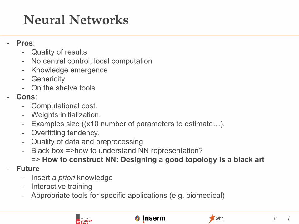
- Pros: - Quality of results- No central control, local computation- Knowledge emergence- Genericity- On the shelve tools
- Cons: - Computational cost. - Weights initialization.- Examples size ((x10 number of parameters to estimate…). - Overfitting tendency. - Quality of data and preprocessing- Black box =>how to understand NN representation?
=> How to construct NN: Designing a good topology is a black art- Future
- Insert a priori knowledge- Interactive training- Appropriate tools for specific applications (e.g. biomedical)

/36
[Lecun et al 2010]
ü Receptive fieldü Hierarchical modelü Max poolingü Layer2layer conn.ü Magnitude factorü Colorü Metamerü Attentionü Local vs Globalü Perspective effectsü Learningü Illusionü Eye mvt
CNN as a model of the visual system …
[Dali 1941][Bacon 1972]
[Nguyen et al CVPR 2015]

/
Illusions - Hallucinations
37
[Ffytche 2007 Dial Clin Neurosc] DeepDream.com

/
New models for neurosciences
38
[Yamins and Dicarlo Nat Neuro 2016]

/39
CNN a model for … auditory cortical responses
For ≠ addednoises
[Kell et al Neuron 2018]
/
Pros
40
• Inform about the nature of the brain encoding not only on the localisation
• Take into account• Distributed nature of information• Statistical dependence between data and stimuli
(specificity increasing)• Use of information contained in weak
activated voxels (sensitivity increasing)• Limit multiple comparison correction

/
Difficulties
41
• Curse of dimensionality: many voxels few observations (examples).
• Limitation of the number of learning categories• Equi-repartition of the predicted variable in the
samples (chunk) for each cross-validation step (fold)
• Importance of paradigm
• With features to use to represent information• Preprocessing (smoothing)?• Generalisation vs discrimination (overfitting)

/
New model of neuroscience
42
from Mike Hawrylycz
How from the activity of millions of neurons distributed in several brain areas emergesimple percepts and how they are linked to emotion, motivation or action?
/
Ivy Glioblastoma Atlas
43
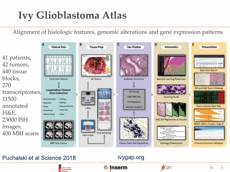
Puchalski et al Science 2018
Alignment of histologic features, genomic alterations and gene expression patterns
ivygap.org
41 patients, 42 tumors, 440 tissue blocks, 270 transcriptomes, 11500 annotated H&E,23000 ISH images, 400 MRI scans

/
Changement de paradigme
44
Data for connectomics (neural networks): 1mm3 rat cortex =>2M Gb =2 x1015=2 Pb=2x103 TB total cortex 500mm3=>103PB (1exabyte, 106 TB)Man = 1000xlarger =103 exabyte (109 TB)(source lichtman et la; Nat Neuro 2014)
Data rate1mm3 =>800h (33j) 2.5 Tb/h => 45y on one machine
[Lichtman et al; Nat Neuro 2014]
UK BioBank100000 subjects (2016-22) 6 MR imaging modalities: tT1w, T2w, swMRI, dMRI, tfMRI, rfMRI2501 individual measures of brain structure and function (2Gb p.sub)1100 other non imaging variablesabout 0.2 PB (200 TB)
[Miller et al; Nat Neuro 2016]
Dermatologists vs CNN127463 biopsies for training 1942 for validationInception v3 (GoogleNet, using several replicas on Nvidia Titan X Gpu)
[Esteva et al Nature 2017]
Ivy Gliobastoma atlas41 patients, 42 tumors, 440 tissue blocks, 270 transcriptomes11500 annotated H&E images23000 ISH images (400 Gb/image), 400 MRI scans
[Puchalski et al Science 2018]

/
AI ó Neurosciences
45
• AI <=Neurosciences• Bio-inspired: NN• Discrimination / Generation
⎼general algorithm for learning⎼ which prior structure ?⎼abstract concept construction⎼ bayesian model
• AI => Neurosciences• Learning hierarchical representation w. a single algorithm• Architecture for testing brain function models (e.g.
consciousness)

/
ML: Natural extension of traditional statistical approaches
46
Deep learningClassic machine learning
Risk calculatorsKnowledge-Based systems
Other
Beam & Kohane Nature 2018

/
Future
47
- Insert a priori knowledge- Interactive training- Transfert learning- Appropriate tools for specific applications (e.g. biomedical)
- Test - the genericity - the robustness to noise (e.g. multicenter studies)- data augmentation- How preprocessing steps influence the results
• Evolving models => regulation & validation

/
Knowledge representation and reasoning for efficient queriesHuman-artefact interaction
[Silver et al Nature 2016]Mixing Hype AI (Supervised L+ Renforcement L) + Old fashion AI (Tree search)
Future

/
if AI gain the trust of healtcare givers & patients
« DL is simply CAD (1990s) on steroids » KopansRadiology 2018
integrate human dimensions with automatedreasoningnew generation of tech savvy physicians
Health-Care penetration

/
Art History
50
Elgammal et al. 2018 arxiv 1801.07729
How characteristics of style are identified?How the patterns evolve?
76921 paintingsTrain(85%)Val (9.5%)Test (5.5%)

/
e-Nosology
51
MS
Stroke.
TBI
ALZ
PD
How characteristics of pathology are identified?How the patterns evolve?
« to discoverfundamental patterns and trends not necessarily apparent to the individualhuman eye »

/
Prediction remains a difficult task ….
52
Groll et al. 2018: https://arxiv.org/abs/1806.03208

/
END …
53
J. Fabre 2012

/
Some references
54
• Context• http://www.andreykurenkov.com/writing/ai/a-brief-history-of-neural-nets-
and-deep-learning/
• Languages• https://www.tensorflow.org/• http://torch.ch/• http://scikit-learn.org/• http://caffe.berkeleyvision.org/• ….
• Courses• Karpathy http://cs231n.github.io/convolutional-networks/• Collège de France : Y Le Cun (2015) et S. Maillard (2019 …)• Ng A https://www.coursera.org/learn/machine-learning• Nielson M. NN & ML http://neuralnetworksanddeeplearning.com/

/
Decoding your mind / Mind reading …
55
[Mur et al SCAN 2009]

/
Pattern recognition
56
Risque d’overfitting
f(x) =w+bf(x*) = wx*+B
[Haynes and Rees Nat Neuro 2006]

/
Mind Reading
57
[Wandell Nature 2008]
Identifying natural images fromhuman brain activityKendrick N. Kay, Thomas Naselaris, Ryan J. Prenger & Jack L. Gallant
Nature Vol 452|20 March 2008
A general brain reading device to access the visual contents of purely mental phenomena such as dreams and imagery

/
Decoding your mind
58
[Haynes and Rees Nat Neuro 2006]
A
AV4h
VWFA

/
Feature selection
59
Which data? Raw data
Convolved data
Estimated data
Whole brain: pb dimensionnalityROI: requires a priori Searchlight analysis
(Kriegeskorte et al. PNAS 2006)
Where?

/
In practice
60
Preprocessing Stat. modelling spm TImage
fMRI time-series
Preprocessing Stat. modelling
TrainfMRI time-series
Preprocessing Stat. modelling
Test
« Leave oneRun one »Crossvalidation
Classif. performanceEach ROIEach sujet

/
Method
61
Temps

/
Method
62
Temps

/
Cortical color representation
63
[Parkes et al. JOV 2009]
Spatial oraganisation of colors in V1,local and sparse
[Brouwer et Heeger J. Neurosci 2009]
- Decoding in V4 > othersGradual transformation of colorrepresentation in ventral areas

/
Water color effect
64
Pinna et al., 2001.

/
Water color effect
65
Gérardin et al. NeuroImage, 2018.

/
Experiment
66
Subjets: 16 subjects (10 women; 28y± 4)fMRI experiments
- fMRI retinotopic mapping
- WCE experiment
Edge
continuity Interior
chromaticity Interior
perceived color
Edge-dependent vs Control
X X
Surface vs Control X X
Surface vs Edge-dependent X X
I II III
V1
0.45
0.5
0.55
0.6
0.65
0.7
0.75
Pred
ictio
n Ac
cura
cy **
I II III
V2
0.45
0.5
0.55
0.6
0.65
0.7
0.75
I II III
V3v
0.45
0.5
0.55
0.6
0.65
0.7
0.75
Pred
ictio
n Ac
cura
cy **
** *
I II III
hV4
0.45
0.5
0.55
0.6
0.65
0.7
0.75 **
** *
I II III
LO
0.45
0.5
0.55
0.6
0.65
0.7
0.75* *
** *
I II III
V3d
0.45
0.5
0.55
0.6
0.65
0.7
0.75
Pred
ictio
n Ac
cura
cy
** *
I II III
V3A
0.45
0.5
0.55
0.6
0.65
0.7
0.75 **
** *
I II III
V7
0.45
0.5
0.55
0.6
0.65
0.7
0.75
**
I II III
V3B/KO
0.45
0.5
0.55
0.6
0.65
0.7
0.75 **
** *
I II III
hMT+/V5
0.45
0.5
0.55
0.6
0.65
0.7
0.75
** *
I: Edge−dependent vs ControlII: Surface−dependent vs ControlIII: Surface−dependent vs Edge−dependent
Retinotopic areas
Ventral visual areas
Dorsal visual areas
I II III
V1
0.45
0.5
0.55
0.6
0.65
0.7
0.75
Pred
ictio
n Ac
cura
cy **
I II III
V2
0.45
0.5
0.55
0.6
0.65
0.7
0.75
I II III
V3v
0.45
0.5
0.55
0.6
0.65
0.7
0.75
Pred
ictio
n Ac
cura
cy **
** *
I II III
hV4
0.45
0.5
0.55
0.6
0.65
0.7
0.75 **
** *
I II III
LO
0.45
0.5
0.55
0.6
0.65
0.7
0.75* *
** *
I II III
V3d
0.45
0.5
0.55
0.6
0.65
0.7
0.75
Pred
ictio
n Ac
cura
cy
** *
I II III
V3A
0.45
0.5
0.55
0.6
0.65
0.7
0.75 **
** *
I II III
V7
0.45
0.5
0.55
0.6
0.65
0.7
0.75
**
I II III
V3B/KO
0.45
0.5
0.55
0.6
0.65
0.7
0.75 **
** *
I II III
hMT+/V5
0.45
0.5
0.55
0.6
0.65
0.7
0.75
** *
I: Edge−dependent vs ControlII: Surface−dependent vs ControlIII: Surface−dependent vs Edge−dependent
Retinotopic areas
Ventral visual areas
Dorsal visual areas

/67
Hebart et al. The Decoding Toolbox (TDT)
FIGURE 3 | Decoding design matrices. (A) General structure of adecoding design matrix. The vertical dimension represents differentsamples that are used for decoding, typically brain images or data fromregions of interest. If multiple images are required to stay togetherwithin one cross-validation fold (e.g., runs), this is indicated as a chunk.The horizontal axis depicts different cross-validation steps or iterations.If groups of iterations should be treated separately, these can bedenoted as different sets. The color of a square indicates whether in aparticular cross-validation step a particular brain image is used. (B)Example design for the typical leave-one-run-out cross-validation (functionmake_design_cv ). (C) Example design for a leave-one-run-out
cross-validation design where there is an imbalance of data in each run.To preserve balance, bootstrap samples from each run are drawn(without replacement) to maintain balanced training data (functionmake_design_boot_cv ). (D) Example design for a cross-classificationdesign which does not maintain the leave-one-run-out structure (functionmake_design_xclass). (E) Example design for a cross-classificationdesign, maintaining the leave-one-run-out structure (functionmake_design_xclass_cv ). (F) Example design for two leave-one-run-outdesigns with two different sets, in the same decoding analysis. Theresults are reported combined or separately for each set which canspeed-up decoding.
Example call (design created and visualized prior to a decodinganalysis as part of the script):
cfg.design = make_design_cv(cfg);% creates the design prior to decoding
display_design(cfg)% visualizes thedesign prior to decoding
Alternative example call (design created and visualized while thedecoding analysis is running):
cfg.design.function.name = ’make_design_cv’;% creates a leave-one-chunk-outcross-validation design
cfg.plot_design = 1;% plots the design when decoding starts
ANALYSIS TYPEMost decoding analyses can be categorized as one of threedifferent types of analysis, depending on the general voxel
selection criterion: Whole-brain analyses, region-of-interest(ROI) analyses, and searchlight analyses. All of these approachesare commonly used for decoding. In the machine learningcommunity, ROI and searchlight analyses might be consideredfeature selection approaches, but this is not typically how they arecalled in the brain imaging community. All of these approacheshave their respective advantages and disadvantages (discussede.g., in Etzel et al., 2009, 2013). Among others, one advantage ofwhole-brain analyses is that all available information is fed intothe classifier, while major disadvantages of this method are thedifficulty to tell the origin of the information and the so-called“curse of dimensionality” (see Table 1). These problems are less ofan issue in ROI analyses, but ROIs need to be specified and can inthat way be biased, variable ROI sizes make them difficult to com-pare, and information encoded across different ROIs gets lost.Searchlight analyses can be seen as a succession of spherical ROIs,but require no prior selection of brain regions and are in thatrespect unbiased to prior assumptions about where to expect an
Frontiers in Neuroinformatics www.frontiersin.org January 2015 | Volume 8 | Article 88 | 7
[Hebart et al. Fninf 2015]
six-fold cross-validation

/
Method
68
DesignMatrix
GLM
Activationforallvisual conditions
Mostactivatedvoxelsineachdelineatedarea
DifferentialtimecoursefortheselectedvoxelsineachROIforeachcondition
p<0.05uncor.
AEdge-Dependentonsets
Controlonsets
Surface-Dependentonsets
C DynamicCausalModeling+BayesianModelSelection
Classification
Six-foldcross
validation
BSupportVectorMachine

/
Results
69
I II III
V1
0.45
0.5
0.55
0.6
0.65
0.7
0.75
Pre
dict
ion
Acc
urac
y
**
I II III
V2
0.45
0.5
0.55
0.6
0.65
0.7
0.75
I II III
V3v
0.45
0.5
0.55
0.6
0.65
0.7
0.75
Pre
dict
ion
Acc
urac
y
**
I II III
hV4
0.45
0.5
0.55
0.6
0.65
0.7
0.75 **
I II III
LO
0.45
0.5
0.55
0.6
0.65
0.7
0.75**
I II III
V3d
0.45
0.5
0.55
0.6
0.65
0.7
0.75
Pre
dict
ion
Acc
urac
y
I II III
V3A
0.45
0.5
0.55
0.6
0.65
0.7
0.75 **
I II III
V7
0.45
0.5
0.55
0.6
0.65
0.7
0.75
I II III
V3B/KO
0.45
0.5
0.55
0.6
0.65
0.7
0.75 **
I II III
hMT+/V5
0.45
0.5
0.55
0.6
0.65
0.7
0.75
I: Edge-dependent vs ControlII: Surface-dependent vs ControlIII: Surface-dependent vs Edge-dependent
Retinotopic areas
Ventral visual areas
Dorsal visual areas
vsvs
vs
nsnsnsnsnsnsns
Multi-Voxel Pattern Analysis (MVPA) from fMRI data.

/
Results
70
Correlating pattern classification and appearance

/
Conclusion
71
– Filling-in is best classified and best correlate with appearance by dorsal areas V3A & V3B/KO
– Uniform chromaticity by ventral areas hV4 & LO– Feedback modulation from V3A to V1 and LO for filling-in– Feedback from LO modulating V1 and V3A for uniform chromaticity
LO
V1
V3A
LO
V1
V3A

/
Dream decoding
72

/
Method
73

/
Method
74

/
Method
75
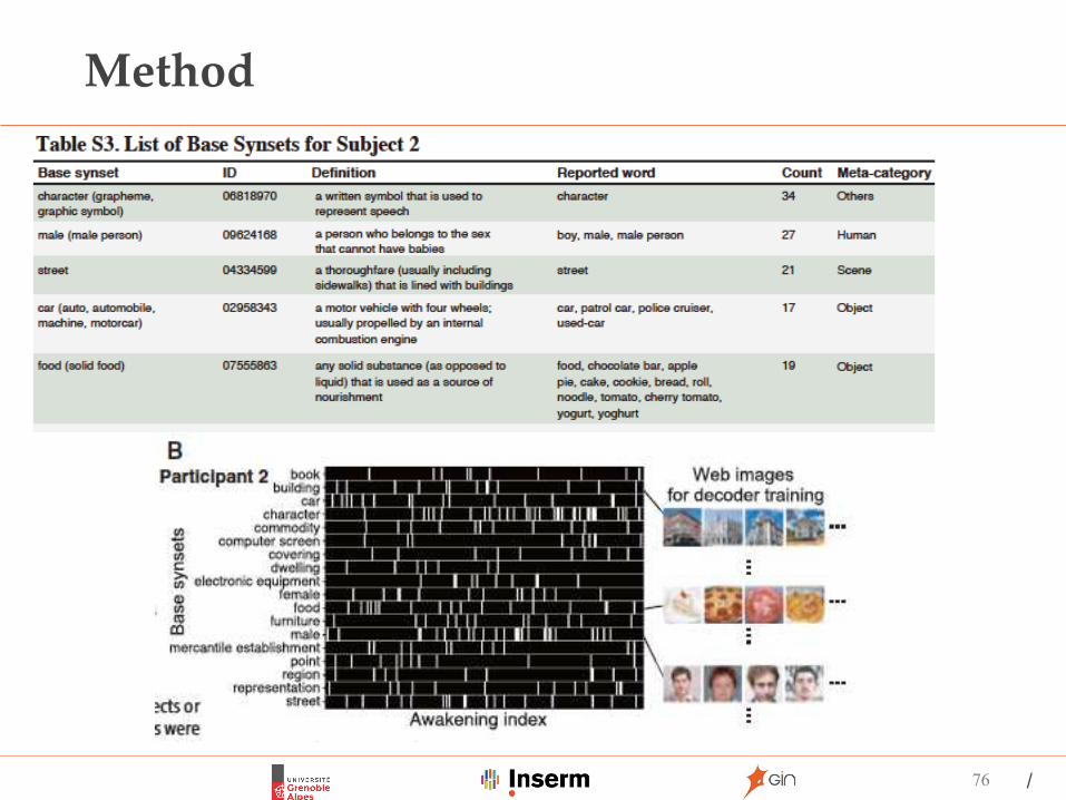
http://image-net.org/
Synset: data elements semanticallyequivalent(synonym set)
/
Method
76

/
Experiment
77
Sleep exp.
Visual exp.

/
Experiment
78
3 sujets (27-39 years)1 pm - 5:30 pmEEG, EOG, EMG, ECGAlpha wave suppression & theta wave occurrence => NREM (stage 1)Hallucinations visuelles (hypnagogiques)3T, 3x3x3 mm, TR=3ssleep exp., 3 volumes before awakeningvisual stimulus exp. (40 blocs 9s + 6s rest, 6 im 0.75s, pour chq base de synsets)
/
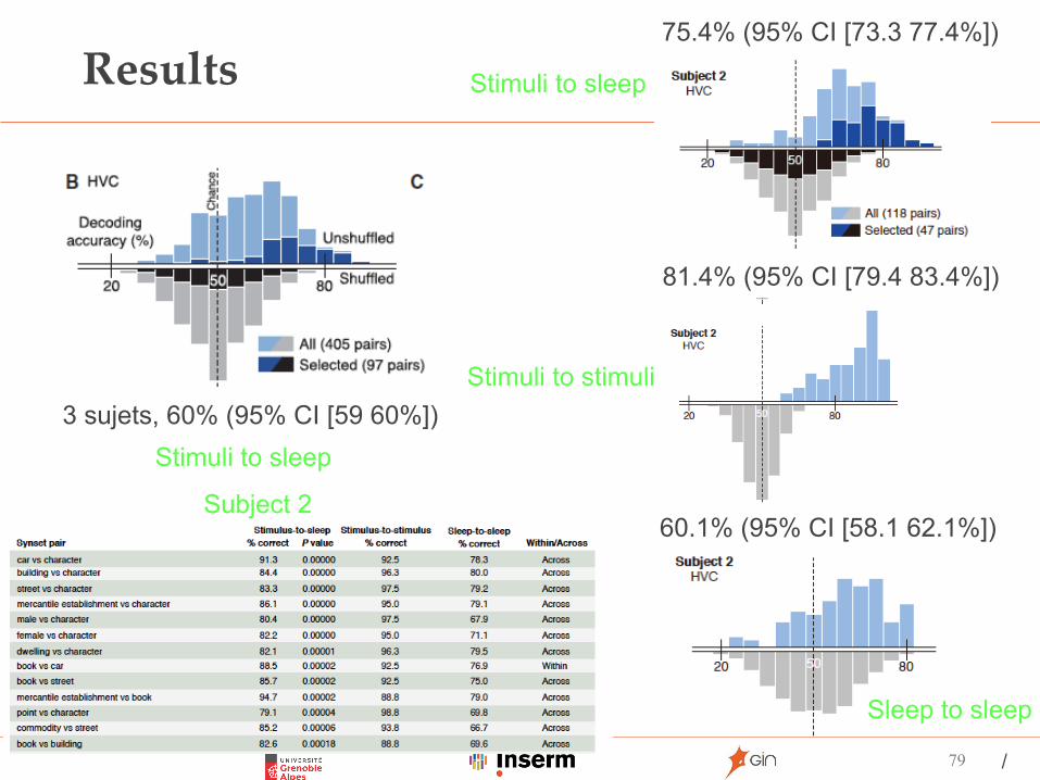
Results
79
3 sujets, 60% (95% CI [59 60%])Stimuli to sleep
75.4% (95% CI [73.3 77.4%])
81.4% (95% CI [79.4 83.4%])
60.1% (95% CI [58.1 62.1%])
Stimuli to sleep
Stimuli to stimuli
Sleep to sleep
Subject 2

/
Results
80

/
Result
81

/82
five out of the eight words were assigned with base synsets(male synset [ID:09624168], male , boy ; female synset[ID:09619168], female , girl , mother ).
“Well, there were persons, about 3 persons, inside some sort of hall. There was a male, a female, andmaybe like a child. Ah, it was like a boy, a girl, and a mother. I don't think that there was any color.”

/83

/
Conclusion
84
üVisual experience during sleep are represented by, and can be read out from, visual cortical activity patterns shared with stimulus representation.
ü Principle of perceptual equivalence a common neural substrate for perception and imagery, generalizes to spontaneously generated visual experience during sleep.
ü Links between verbal reports and fmri patterns using MVPA, lexical and image databases.
ü Semantic decoding with the HVC does not rule out the possibility of decoding low-level features with the LVC.
ü The same decoders could also be used to decode REM imagery.