machine learning in disruption-tolerant manetsboxu/mp2p/taas-malena-final-appearance.pdf · that is...

P1: OJL

TAAS040A-23 ACM-TRANSACTION November 6, 2009 5:27

23

Machine Learning in Disruption-TolerantMANETs

BO XU

University of Illinois at Chicago

OURI WOLFSON

Pirouette Software Consulting and University of Illinois at Chicago

and

CHANNAH NAIMAN

Pirouette Software Consulting

In this article we study the data dissemination problem in which data items are flooded to allthe moving objects in a mobile ad hoc network by peer-to-peer transfer. We show that if memoryand bandwidth are bounded at moving objects, then the problem of determining whether a set ofdata items can be disseminated to all the moving objects is NP-complete. For a heuristic solutionwe postulate that a moving object should save and transmit the data items that are most likelyto be new (i.e., previously unknown) to future encountered moving objects. We propose a methodto be used by each moving object to prioritize data items based on their probabilities of beingnew to future receivers. The method employs a machine learning system for estimation of thenovelty probability and the machine learning system is progressively trained by received dataitems. Through simulations based on real mobility traces, we show the superiority of the methodagainst some natural alternatives.

Categories and Subject Descriptors: H.2.4 [Database Management]: Systems—Distributeddatabases; C.2.4 [Computer-Communication Networks]: Distributed Systems—Distributeddatabases; distributed applications

General Terms: Algorithms, Performance

Additional Key Words and Phrases: Mobile data management, mobile ad hoc networks, publish/subscribe, resource discovery, mobile peer-to-peer networks

This research was supported by NSF grants DGE-0549489, 0513736, 0326284, OII-0611017.Authors’ addresses: B. Xu, Department of Computer Science, College of Engineering, Universityof Illinois at Chicago, IL; email: [email protected]; O. Wolfson, Pirouette Software Consulting, De-partment of Computer Science, College of Engineering, University of Illinois at Chicago, IL; email:wolfson@ cs.uic.edu; C. Naiman, Pirouette Software Consulting, Chicago, IL; email: [email protected] to make digital or hard copies of part or all of this work for personal or classroom useis granted without fee provided that copies are not made or distributed for profit or commercialadvantage and that copies show this notice on the first page or initial screen of a display alongwith the full citation. Copyrights for components of this work owned by others than ACM must behonored. Abstracting with credit is permitted. To copy otherwise, to republish, to post on servers,to redistribute to lists, or to use any component of this work in other works requires prior specificpermission and/or a fee. Permissions may be requested from Publications Dept., ACM, Inc., 2 PennPlaza, Suite 701, New York, NY 10121-0701 USA, fax +1 (212) 869-0481, or [email protected]© 2009 ACM 1556-4665/2009/11-ART23 $10.00DOI 10.1145/1636665.1636669 http://doi.acm.org/10.1145/1636665.1636669

ACM Transactions on Autonomous and Adaptive Systems, Vol. 4, No. 4, Article 23, Publication date: November 2009.

P1: OJL


23:2 • B. Xu et al.

ACM Reference Format:

Xu, B., Wolfson, O., and Naiman, C. 2009. Machine learning in disruption-tolerant MANETs. ACMTrans. Autonom. Adapt. Syst. 4, 4, Article 23 (November 2009), 36 pages.DOI = 10.1145/1636665.1636669 http://doi.acm.org/10.1145/1636665.1636669

1. INTRODUCTION

A mobile ad hoc network (MANET) is a network of autonomous moving objectsconnected by short-range wireless links such as 802.11 or Bluetooth. A MANETthat is subject to frequent disconnections is sometimes called a Disruption-Tolerant Network (DTN)1 (see, e.g., Burns et al. [2005]). In this article we con-sider two application scenarios in a MANET or a DTN, namely routing anddissemination. In the routing scenario, a message is delivered from a sourceobject to a specific single destination object. In the dissemination scenario, amessage is delivered from a source object to all the objects in the system. Anapplication example for the dissemination scenario is as follows. The movingobjects (PDAs and/or vehicles) carry sensors which monitor the environment,for example, take pictures to detect intruders, sense available parking slots, orconcentrations of various substances in the air. Assume that the set of valuessimultaneously sensed by a moving object O constitute a data item generatedby O, and for reliability and functionality (so that each user has a local databaserepresenting the neighborhood) each data item has to be disseminated to allthe moving objects. Since the ranges of 802.11 or Bluetooth are not sufficientto reach all moving objects, the dissemination is done by transitive multihoptransmission.

There are two paradigms to conduct this dissemination, namely structuredand structureless. In structured dissemination, a relay structure such as atree is imposed and maintained among the moving objects (e.g., Huang andGarcia-Molina [2004]). Structured dissemination may be very ineffective in ahighly mobile MANET, in which the routing structure quickly becomes obso-lete. In structureless dissemination, the intermediate objects save data itemsand later (as new neighbors are discovered) transfer these data items. In theliterature this paradigm is also called structureless gossiping [Jelasity et al.2004; Friedman et al. 2007; Birman et al. 1999], epidemic [Vahdat and Becker2000], or store-and-forward dissemination [Sormani et al. 2006].

Since there is no central control point, each moving object needs to decidewhen a data item has already been communicated to all the other moving objectsin the system and therefore can be dropped. To do so, each moving object needsto collect information, analyze it, and decide whether to drop a data item fromcommunication or from memory. This leads to the autonomic control loop, asintroduced in Dobson et al. [2006].

We first formalize the data dissemination problem, and consider it in an idealenvironment where all the trajectories of moving objects are known a priori ata centralized location. We show that if memory and bandwidth are bounded at

1DTNs is a newer term, favored by DARPA (Defense Advanced Research Projects Agency) overdelay-tolerant networks.


P1: OJL


Machine Learning in Disruption-Tolerant MANETs • 23:3

moving objects, then the problem of determining whether a set of data items canbe disseminated to all the moving objects is NP-complete (although we showthat the problem can be solved efficiently if memory and bandwidth are un-bounded). Thus in a distributed/mobile environment, where information suchas the trajectory of a moving object is usually unknown to other objects, we re-sort to heuristics. More specifically, in our scheme each moving object prioritizesthe data items in order to accommodate them in limited bandwidth and memory.

In particular, we postulate that an important factor that determines thepriority of a data item is its current novelty probability, that is, its probability ofbeing new (i.e., previously unknown) to an arbitrary moving object encounteredin the future. The reason is that the transmission of data items that are alreadyknown wastes bandwidth, memory, and power. Thus, in this article data itemsare ranked based on their current novelty probability.

Under uniformity assumptions, the novelty probability of a data item R ata particular time is simply the ratio between the total number moving objectsthat have received R, and the total number of moving objects in the system.Unfortunately, a parametric formula giving the novelty probability is beyondthe state-of-the-art. Results from epidemiology and random graphs may beuseful in deriving such a formula, but they can’t be applied directly. Even ifsuch a formula existed it would depend on global parameters of the environmentsuch as the turnover rate (i.e., the rate at which moving objects enter and exitthe system) which are normally unknown to individual objects. To introducethe approach proposed in this article observe that the novelty probability of adata item R depends on attributes of R (e.g., its age), as well as global systemparameters such as the turnover rate. The attributes of R that can affect itsnovelty probability are called novelty indicators.

In this article we show that, unfortunately, no single indicator is a good pre-dictor of novelty in all environments. For example, in some environments theintuition that the age of the data item is a good predictor of novelty is correct. Inother words, the older the data item, the more likely it is that an arbitrarily en-countered object already knows it. However, consider an environment in whichthe turnover rate of moving objects is high; namely, many new moving objectsare entering the system. In this case, even though the data item is old, it may notbe known to the numerous objects that are new in the system. In this case, weshow that the number of times a data item is received by a moving object is a bet-ter indicator of novelty to future-encountered objects than age. This variabilityis a problem since a moving object normally does not know the global parame-ters of the environment in which it operates. For example, it does not know if themoving object’s turnover is high or low. Currently, a complete characterizationof environments and novelty-indicators is beyond the state-of-the-art.

Previous work on dissemination in mobile ad hoc networks has studied var-ious heuristics for reducing redundant transmissions, but each using a singleindividual novelty indicator. For example, Ni et al. [1999] considers the numberof receptions and distance separately; Hayashi et al. [2003] and Burges et al.[2006] consider the number of hops.

In this article we propose a method that combines various novelty indica-tors in order to estimate the novelty probability. The combination uses machine


P1: OJL


23:4 • B. Xu et al.

Collect

Analyze

Decide

Act

Training set: NIV’s of received data-items + “old’/”new” labels

Learning system trained

and improved

Learning system used to decide which data-items to save

or which data-items to transmit

Data-items saved

or transmitted

Collect

Analyze

Decide

Act Learning system trained

and improved

Learning system used to decide which data-items to save

or which data-items to transmit

Data-items saved

or transmitted

Fig. 1. The autonomic control loop formed by the MALENA method.

learning in a method called MALENA (MAchine LEarning-based Novelty rAnk-ing). The method infers from previously received data items what the indicatorsof a new data item “look like.” In other words, it learns the novelty probabilitybased on the novelty indicators. For this purpose, the set of novelty indicatorsof a data item R, called the Novelty Indicator Vector (NIV) of R, are transmit-ted by each moving object together with the data item. This will increase thesize of the data item by only a few bytes and it is negligible considering thatdata items containing, say, the picture of a conventioneer, may have a length oftens of Kbytes. The receiver of R determines whether or not R is new, and therespective NIV becomes a training example. In other words, the receiver treatsitself as an arbitrary moving object that will be encountered in the future. Thus,a moving object progressively collects a training set which improves its learningsystem. When the object ranks its database to decide which data items to keepin memory or which data items to transmit, the learning system is used to cal-culate the novelty probability. Furthermore, using a sliding window of examplesMALENA can adapt to new environments. In this sense MALENA provides amethod that allows building Autonomic Communication (AC) algorithms (seeVasilakos et al. [2009]) that dynamically adapt to changing conditions or con-text. In summary, the execution of MALENA forms an autonomic control loop(see Dobson et al. [2006]) as shown in Figure 1.

Observe that it is possible to design some specific data dissemination algo-rithms that consider multiple parameters simultaneously, estimate parame-ters that cannot be measured directly, and adapt in sophisticated ways. How-ever, MALENA provides a generic method in the sense that environmentsoptimized by new novelty indicators can be considered simply by adding thenew indicator to the machine learning system. Also, different machine learn-ing algorithms can be “plugged-in” the method. (In this article we instanti-ate the method with the two novelty indicators aro and fin discussed shortly,and with Bayesian machine learning). Furthermore, as we discuss at theend of the Introduction, the method can augment different store-and-forwardalgorithms.


P1: OJL



We compare MALENA with three approaches to ranking of data items. In thefirst two approaches, ranking is based on a single individual novelty indicator.Specifically, the aro-ranking approach ranks data items based on the order inwhich they arrive at a moving object, and the fin-ranking approach ranks a dataitem based on the number of times it is received by the moving object. We choosethese two indicators because each of them is found to be an optimal indicatorin an environment that is not favorable to the other. The third approach isPeopleNet [Motani et al. 2005]. We compare MALENA with these methods inboth the dissemination scenario (i.e., all destinations) and the routing scenario(i.e., single destination).

Orthogonal to the application dimension, we compare the methods undertwo gossiping protocols, push gossiping and push-pull gossiping. In the pushgossiping, two encountering moving objects directly exchange the data items intheir local databases. In push-pull gossiping, the gossiping protocol follows twophases. In the first phase, the encountering moving objects exchange the ids ofthe data items in their local databases. In the second phase, they exchange thedata items that are new (unknown) to the peer.

The performance measure that we propose is also novel. It integrates twoexisting evaluation metrics for data dissemination, namely throughput anddelivery time, with the purpose of providing a single criterion for comparison.Thus the performance measure reflects both how many distinct data items arereceived by each moving object during its trip, and how soon they are received.The comparison of the methods is done by simulation, where we use traces ofreal Bluetooth sightings at a conference. We also evaluated MALENA usingsynthetic 802.11 traces.

The performance study indicates that, in either the dissemination or the rout-ing scenarios, and with either push gossiping or push-pull gossiping, there areenvironments for which age is a better novelty indicator than fin (in the sensethat it has better performance), and there are other environments for whichthe opposite is true. However, MALENA always approaches or outperforms thebest indicator in each individual environment, and therefore performs well inboth. This demonstrates the power of combining the novelty factors and theadaptability of machine learning to the environment.

The approach enables us to argue about other novelty indicators as follows. Inthe existing literature on DTNs and MANETs, various assumptions are used,each typical to an environment. For example, some papers assume that themoving objects have GPS and thus know their locations [Lebrun et al. 2005;Burns et al. 2005], that the future trajectories of all the moving objects and thefuture communication traffic demand are known a priori [Jain et al. 2004], thatmoving objects have fixed periodic trajectories such as buses [Zhao et al. 2005],that the communication network is always connected [Karp and Kung 2000],and that the mobility of some peers can be controlled by the dissemination al-gorithm [Li and Rus 2000]. Subsets of assumptions may produce environmentsfor which different indicators are superior, and moreover, a moving object maynot know the parameters of the environment in which it is operating. In thiscase MALENA can be used to provide a performance that is close to optimalregardless of the environmental parameters.


P1: OJL


23:6 • B. Xu et al.

Finally, an important comment is that MALENA is a method of improvingrouting and dissemination, rather than an algorithm, in the sense that it canbe combined with other routing and dissemination algorithms. We explainedbefore that the method enables the incorporation of other novelty indicators.Furthermore, the novelty probability computed by MALENA is orthogonal toand can be combined with other measures of data item priority such as size.Specifically, if data items have different sizes, then ranking can be done basedon the novelty probability per byte, that is, the novelty probability divided bythe size. Similarly, if data items have different reliability or popularity factors,the novelty probability can be multiplied by such a factor to compute the rank.Another orthogonal issue is bandwidth allocation, namely how many data itemsshould a moving object transmit during a peer-to-peer interaction. This is im-portant in a dense environment where collisions are a major concern and/or in ahighly mobile environment where the communication time between encounter-ing objects is limited. Again MALENA can be combined with any bandwidth al-location scheme in the sense that once the bandwidth allocation is determined,MALENA can be used to select the data items to transmit in such allocation.For an example of a bandwidth allocation scheme, see Wolfson et al. [2006b].Yet another orthogonal issue is which moving objects to exchange data itemswith. For the sake of scalability, a moving object may not necessarily exchangewith every encountered object. Gossiping protocols have developed randomizedmechanisms for a moving object to select a subset of the encountered objectsto exchange with (see, e.g., Jelasity et al. [2004], Friedman et al. [2007], andBirman et al. [1999]). Once this subset is determined, MALENA can be used toselect the data items to transmit. In general, MALENA provides a method forestimating novelty probabilities, and it can be incorporated into and augmentany algorithm that addresses many other aspects of data dissemination in mo-bile ad hoc networks, including bandwidth allocation, collision management,gossiping protocols, and data item prioritization.

The rest of the article is organized as follows. Section 2 formalizes the prob-lem and analyzes it theoretically. Section 3 describes the MALENA method,and Section 4 evaluates MALENA by simulations, under the push gossiping.Section 5 describes and evaluates MALENA under push-pull gossiping. Sec-tion 6 discusses related work, and Section 7 concludes the article and discussesfuture work.

2. THE MOVING OBJECTS DATA DISSEMINATION (MODD) PROBLEM

In this section we define and analyze the MODD problem in the centralizedcase. We show that the problem can be solved efficiently when there are noresource constraints, but is intractable otherwise. In Section 2.1 we introducethe model, in Section 2.2 we discuss P2P communication, and in Section 2.3 weanalyze the two MODD variants.

2.1 The Model

Our system consists of a finite set of point (i.e., without an extent) moving ob-jects. Each object O has a memory allocation and a bandwidth/energy allocation


P1: OJL



that are dedicated to data item dissemination. Bandwidth and energy imposeconstraints on how much a moving object can transmit during a peer-to-peerinteraction and therefore we consider them collectively. The motion of movingobject O is represented by a trajectory that defines the location of O as a func-tion of time. For example, the motion can be approximated arbitrarily close bya piecewise linear function defined as follows.

Definition 1. A trajectory is a polyline in three-dimensional space (two-dimensional geography, plus time), represented as a sequence of points(x1, y1,t1), (x2, y2,t2), . . . , (xn, yn,tn) (t1 < t2 < . . . < tn). The object is at (xi, yi)at time ti, and during each time interval [ti,ti+1], the object moves alonga straight line from (xi, yi) to (xi+1, yi+1), and at a constant speed given by

vi =√

(xi+1−xi )2+( yi+1− yi )2

ti+1−ti. Thus, given a trajectory Tr, the location of the object

at a point in time t between ti and ti+1 (1 ≤ i ≤ n) is obtained by a linearinterpolation between (xi, yi) and (xi+1, yi+1). We denote by Tr(t) the location ofTr at time t.

Any other (i.e., nonlinear) function that gives the (x, y) location of a movingobject as a function of time is satisfactory for the purpose of this article.

Occasionally, a moving object O produces a data item R having some uniqueitem-id, and a size s(R). For example, the data item is an image taken by themoving object. The uniqueness of the item-id can be achieved by, for example,the combination of the MAC address of O (which is globally unique) and asequence number that monotonically increases for each data item produced byO. For simplicity we assume that all data items have the same size. A dataitem can also be called a tuple. O is called the producer of R. With each dataitem is associated a timestamp called the produce-time, indicating the time atwhich R is produced. In our model time is local to each moving object, and isrepresented as a sequence number, starting from 1.

Each moving object O maintains a database which can hold MO data items.Each O uses the data items that it needs when they are received from othermoving objects (see next subsection), or when O produces them. The databaseis maintained solely for the purpose of disseminating the data items to othermoving objects.

In addition, O has a memory area called the buffer that is common to allthe applications running on the moving object. We assume that the size of thebuffer is at least MO .

2.2 Peer-to-Peer Data Dissemination

Moving objects communicate via short-range wireless communication networks(such as Bluetooth or 802.11), having a transmission range d. Thus, pairwisecommunication can occur between two moving objects while the distance be-tween them is at most d . When two moving objects A and B encounter each other(i.e., when the distance between them becomes smaller than d ), they engagein a data items exchange. In Bluetooth, encounter detection is a built-in fea-ture of the protocol. In 802.11, an encounter can be detected by periodical hellomessages. The sets of data items exchanged depend on the bandwidth/energy


P1: OJL


23:8 • B. Xu et al.

of each moving object, the memory allocation of each, and the period of time forwhich they stay within transmission range. For brevity we omit a formal def-inition of a pairwise data items exchange; but it has to respect the bandwidthand memory allocations of each moving object.

We first consider the centralized version of the Moving Objects Data Dissem-ination (MODD) problem which can be defined as follows.

Definition 2 (The MODD Problem). Given:

—a set of moving objects MO, each having a trajectory, a bandwidth/energy,and a memory allocation; and

—a data items production schedule S, that is, a set of data items, each of whichhas a size, a producing moving object, and a production time.

Can each data item in the schedule S be received by all the moving objects inMO by a sequence of data items exchanges?

Observe that due to resource (memory and bandwidth/energy) limitations, itis possible that each one of two data items in the schedule can reach a movingobject O, but both cannot do so. For example, suppose that in order to reach Oboth data items have to be carried simultaneously by another object P , but Phas enough storage for only one data item. More specifically assume that theonly object that comes within transmission range of O is P , and the only timeinterval when it does so is 7:00 to 7:02. Furthermore, during this time intervalP does not come within transmission range of any other object, except for O.Then, only one data item can reach O.

2.3 Variants of the MODD Problem

In this subsection we demonstrate that the MODD problem can be solvedefficiently if bandwidth/energy and memory are unlimited, but becomes NP-complete when such limitations are introduced.

2.3.1 Unbounded Resources. First we consider the variant of the problemin which memory and bandwidth/energy are unlimited, and we show that in thiscase the MODD problem can be solved in polynomial time. Specifically, we showthat there is an efficient algorithm to determine whether a given data item canreach a given moving object; and since resources are unlimited, reachability ofone data item is independent of another, and thus a set of data items can reachall the moving objects if each data item can reach some moving object in theset.

If bandwidth is unlimited the transmission time of a data item is zero. Notethat even when resources are unbounded, a data item produced by a movingobject cannot reach another moving object. For example, this is the case whenthere are only two moving objects which do not encounter each other.

We start with the following definition of the contact graph, which is a tool thatwill enable us to determine the set of moving objects that a data item can reach.

Definition 3. Let dis(p,q) denote the distance between location p and lo-cation q. A contact interval between two trajectories Tri and Tr j (of moving


P1: OJL



objects i and j ), denoted Lij (s,e), is a time interval [s,e] such that:

(1) for any time point t ∈[s,e], dis(Tri(t),Tr j (t)) ≤ d . (Recall that Tri(t) andTr j (t) are the locations of i and j at t interpolated by Tri and Tr j respec-tively; and d is the transmission range), and

(2) if there exists a time point t < s (or t > e) such that dis(Tri(t),Tr j (t))≤ d , then there exists a point t ′ such that t < t ′ < s (or e < t ′ < t) anddis(Tri(t ′),Tr j (t ′)) > d . This indicates that the time interval is maximal inthe sense that it cannot be extended.

Intuitively, a contact interval is a continuous time interval where the movingobjects represented by the two trajectories are within the transmission rangeof each other.

Given a pair of trajectories, it can be determined in quadratic time usingstandard computational geometry techniques what are their contact intervals.

Definition 4. The contact graph is an undirected labeled multigraph, whereeach node i represents a moving object i, and each link Lij (s,e) represents acontact interval between i and j .

Note that there can be multiple links between i and j , each correspondingto one contact interval.

Example 1. Figure 2 gives an example contact graph of four objects A, B,C, D. There are two contact intervals between A and B, indicating that they en-counter each other from 9:30 to 9:35 and from 13:15 to 13:20. Similarly, the con-tact graph gives the contact intervals between A and C, C and D, and B and D.

Given a contact graph and a data item produced by a moving object O at atime t, the reachability set of the data item is defined using the concept of theearliest arrival time at a moving object. Intuitively, the earliest arrival time ata moving object N is earliest time at which the data item can reach N. Formally,the earliest arrival time of nodes in the contact graph is defined recursively bythe following algorithm.

Initially the earliest arrival time at each node except O is set to infinity. Theearliest arrival time at O is t. The earliest arrival time is updated for a neighborN of O if there is an edge LNO(s,e) such that e is higher than t. In this case, letb be the minimum e among all such edges between N and O, and denote thatedge by LNO(a,b). (Intuitively, (a,b) is the earliest time interval during which thedata item can be transmitted from O to N .) Let w be the maximum between aand t. The new earliest arrival time at N is the minimum between the existingearliest arrival time at N and w. The process is repeated for every neighborN of O, and then O is marked “examined”. Then the previous procedure isrepeated starting from the unexamined node with the smallest earliest arrivaltime, until there are no unexamined nodes.

For some nodes of the graph the earliest arrival time may remain infinity atthe end of the preceding algorithm. The reachability set of a data item is theset of moving objects that have a finite earliest arrival time.

Example 1 (continued). From Figure 2 we can see that D is reachable by adata item produced by A at any time before 9:30. One possible routing scheme


P1: OJL


23:10 • B. Xu et al.

A B

C D

[9:30, 9:35]

[13:15, 13:20]

[10:00, 10:10][11:20, 11:26]

[8:30, 8:32]

Fig. 2. An example contact graph.

is that A forwards the data item to B when A encounters B at 9:30, and then Bforwards to D when B encounters D at 10:00. However, a data item producedby A at any time after 9:35 cannot reach D, via either B or C. It cannot reachvia B because after 9:35 A encounters B after B encounters D. Similarly, thedata item cannot reach via C because A encounters C after C encounters D.

THEOREM 1. Assume that we are given a contact graph, and a data itemR produced by a moving object i at time t. The reachability set of R can bedetermined in time which is quadratic in the size of the contact graph.

Since in an unbounded resource instance of the MODD problem, the reach-ability set of one data item is independent of the set of other data items in thedata items production schedule, we have the following.

COROLLARY 1. Given a set of trajectories of size n, and a data items produc-tion schedule of m data items, the MODD problem can be solved in time O(mn2).

2.3.2 Bounded Resources.

THEOREM 2. Given bounds on memory and bandwidth for processors, theMODD problem is NP-complete.

PROOF (SKETCH). The reduction is from the Multiprocessor Scheduling (MS)problem (see Garey [1979]). The complete proof is provided in Appendix A.

Note that the bounded resource MODD problem is NP-complete even in thecentralized case in which all the parameters are given a priori (i.e., all the tra-jectories and data item producers are known). In the distributed case a movingobject usually does not know these parameters. Therefore, in the mobile casewe will resort to heuristics that use machine learning.

Although there are many results for related problems in scheduling andnetwork flow, we do not believe that the MODD problem has been solved.

3. NOVELTY PROBABILITY

In this section we discuss how to compute the probability for a data item to benew to future encountered objects. In Section 3.1 we discuss the indicators thatwill be used in computing the novelty probability, in Section 3.2 we discuss theMachine Learning (ML) framework, in Section 3.3 we discuss how to manage


P1: OJL



the space overhead of the ML framework, and in Section 3.4 we discuss the useof the Bayesian machine learning algorithm in the framework.

3.1 Novelty Indicators

Consider the time when a moving object O assigns a rank to a data item R. Wepostulate that the probability that R will be new to the moving objects that willbe encountered in the future by O depends on several elements called noveltyindicators. The following are two possible novelty indicators.

(1) The relative order in which R arrives at O. This indicator is called thearrival order, and is denoted by aro. Specifically, if R is the kth data itemthat arrived at O (among all the data items in the current database), thenthe arrival order of R is k. Clearly 1 ≤ aro ≤ MO (recall that MO is thenumber of data items in O ’s database). A small arrival order suggests thatR has been in the database for a relatively long time and thus has probablybeen in the system longer, and also has been transmitted by O more timesthan other data items. Therefore a small arrival order would indicate a lowprobability of future novelty.

(2) The number of times R has been received by O from other moving objects,denoted by fin. The higher fin, the less likely that R is new to O ’s futureencountered objects, since this means that R has already been widely dis-seminated by other moving objects.

This set is by no means exhaustive. One can easily come up with other noveltyindicators, such as the number of hops R has traveled before it reaches O, thenumber of times R has been transmitted by O, and the age of R. However,the method that we propose in this article is able to integrate these and otherindicators. Moreover, we considered other indicators and found that amongthem aro or fin are superior for the environments examined in this article.

Given a data item R at a moving object at a particular time, the pair (aro,fin) is called the Novelty Indicator Vector (NIV) of R.

3.2 Computation of Novelty Probability Using Machine Learning

In this subsection we introduce a framework for using machine learning tech-niques to predict the novelty probability based on a novelty indicator vector.This is a general framework in the sense that different ML systems can beplugged into it.

ML intuitive framework. Suppose that we are given a multiset ES of ex-amples, where each example is a pair (X, label) and the same example mayappear multiple times in the set. X is a NIV and label is either “new” or “old.”The “new” indicates that the data item associated with the NIV X was new atthe receiving moving object (i.e., the object has never received the data itembefore). And similarly, “old” indicates that the associated data item was notnew.

A machine learning system Q is a function of the examples set ES and a NIVX. Particularly, Q(ES, X) returns the probability that a data item with NIV X

will be new to encountered objects in the future, given the examples set ES.


P1: OJL


23:12 • B. Xu et al.

Database of O

item-iddata-item

descriptionaro fin

R1 … … 1 1

R4 … … 2 4

R2 … … 3 2

R7 … … 4 2

transmission

set

Tracking set

of O

item-id

R2

R1

R3

R7

R4

R6

produce-time

Database of O

item-iddata-item

descriptionaro fin

R1 … … 1 1

R4 … … 2 4

R2 … … 3 2

R7 … … 4 2

transmission

set

Tracking set

of O

item-id

R2

R1

R3

R7

R4

R6

produce-time

Fig. 3. Three sets of tuples (Database, Tracking set, Transmission set) maintained in a movingobject O.

The examples set ES is collected as follows. When a data item R is transmit-ted, the sender attaches to R the NIV of R that is maintained by the sender.For each received data item, the receiver determines whether it is new to thereceiver, and the respective NIV, along with the label “old” or “new”, becomesan example in the receiver’s ES set.

Old/new labeling and the tracking set. Now we elaborate on the old/newlabeling of the examples collected by the previous framework. Observe thata data item may be received, then purged from the database, then receivedagain. It would be false to label the data item “new” in the second receipt.But this is exactly what O would do if the label is determined by simply con-sidering the database. Thus, O keeps a tracking set, in which each entry isthe item-id (i.e., the unique identification) of a data item that has been re-ceived at O. An entry in the tracking set survives even when the correspondingdata item is purged from the database. And when a data item is received, itsitem-id is searched in the tracking set for labeling, and thus “false” labeling isavoided.

Observe also that the size of each entry in the tracking set is only a fewbytes, thus the tracking set can contain many more tuples than the database.Furthermore, as we discuss later in this subsection, the size of the tracking setcan be bounded.

In summary, the MAchine-LEarning-based Novelty rAnking (MALENA) sys-tem distinguishes among four sets of tuples pertaining to data items. The track-ing set described earlier pertains to all the data items ever received by a movingobject; the database contains the data items that are currently stored by themoving object, which in turn is a subset of a tracking set; the transmissionset is the subset of the database which is transmitted in an encounter. ObjectO also keeps the set ES of all the examples O has received. (As we will seelater when we plug in the Bayesian machine learning system, O actually onlyneeds to remember a limited amount of aggregate data about ES (e.g., the num-ber of “new-data item” examples that have been received and so on), withoutremembering any actual example in ES.) The first three sets are demonstratedin Figure 3, and the examples set is demonstrated in Figure 4.

Formally, the pseudocode of the MALENA method is as follows.


P1: OJL



Algorithm 1. MALENA, executed at a moving object O, when O encounters anothermoving object A

Input: DBO – the database at OTSO – the tracking set at OQ – the machine learning system at Ok – the size of the transmission set to be sent by O. // The value of k is deter-

mined by the bandwidth/energy allocation and the data item size.MO – the size of the database at OG – the transmission set received from A

Output: F – transmission set sent from ODBO – updated database at O

1. for each R in DBO , compute the novelty probability of R using Q2. F ← topK(DBO , k)

// Sort the data items in DBO in decreasing order based on their novelty probabilities.// Select the top k data items (i.e., k items with highest probabilities).

3. Transmit the data items in F and their NIV’s to A4. Receive G the transmission set from A in exchange5. for each R in G, do aro ← arom, where arom = 1+(the current maximum aro in

DBO ).6. for each data item R and its NIV X received from A, do

Create an example (X, label) where label is “new” if the item-id of R does not existin TSO , and “old” otherwise.INSERT EXAMPLE((X,label))// Add the example (X, label) to the examples set. INSERT EXAMPLE is implementedby the machine learning system Q and it is where Q is actually trained. After theINSERT EXAMPLE is finished, (X, label) is discarded. The INSERT EXAMPLEprocedure for Bayesian learning is described in the next subsection.if R is new to O, then

Create an entry (R ’s-item-id, Y) in TSO, where Y is the NIV: (arom, fin = 1)else // R is not new to O

Update the NIV of R in TSO by increasing its fin value by 1.

7. DBO ← topK(DBO ∪ G, MO )// Sort the data items in G together with the data items in DBO , in decreasing orderof their novelty probabilities (computed by the machine learning system Q ; see theintuitive framework at the beginning of this subsection); save the top MO data itemsin DBO . Reports in G that are labeled as “old” in step 6 are discarded directly, withoutparticipation in sorting.

8. The aro values of the data items in DBO are adjusted to start from 1 and to eliminatethe gaps created by the data items that did not fit in DBO .

As we will see in the next subsection, the time complexity of the IN-SERT EXAMPLE procedure is a constant. Assuming that the tracking set isaccessed by using a hash table, step 6 can also be executed in constant time.Thus the complexity of the MALENA method is dominated by the sorts in steps2 and 7, and is O(MlogM), where M is the number of data items in the database.


P1: OJL


23:14 • B. Xu et al.

aro fin label

1 4

2 1

old

new

Examples created from

data-items in message

(a)

(b)

(c)

(d)

Before receiving

After receiving

Example set ESof O

insert

item-iddata-item

descriptionaro

R1 … 1

R2 … 2

Database of O

R1

R2

item-id

R3

Tracking set

of Ofin

5

3

R1

R2

item-id

R3

Tracking set

of O

R4

produce-

time

…

…

item-iddata-item

descriptionaro

R1 … 1

R2 … 2

Database of O

fin

5

1

produce-

time

…

…

item-iddata-item

descriptionaro

R3 … 1

R4 … 2

Message received from a peer

fin

4

1

produce-

time

…

…

aro fin label

1 4

2 1

old

new

Examples created from

data-items in message

(a)

(b)

(c)

(d)

Before receiving

After receiving

Example set ESof O

insert

item-iddata-item

descriptionaro

R1 … 1

R2 … 2

Database of O

R1

R2

item-id

R3

Tracking set

of Ofin

5

3

R1

R2

item-id

R3

Tracking set

of O

R4

produce-

time

…

…

item-iddata-item

descriptionaro

R1 … 1

R2 … 2

Database of O

fin

5

1

produce-

time

…

…

item-iddata-item

descriptionaro

R3 … 1

R4 … 2

Message received from a peer

fin

4

1

produce-

time

…

…

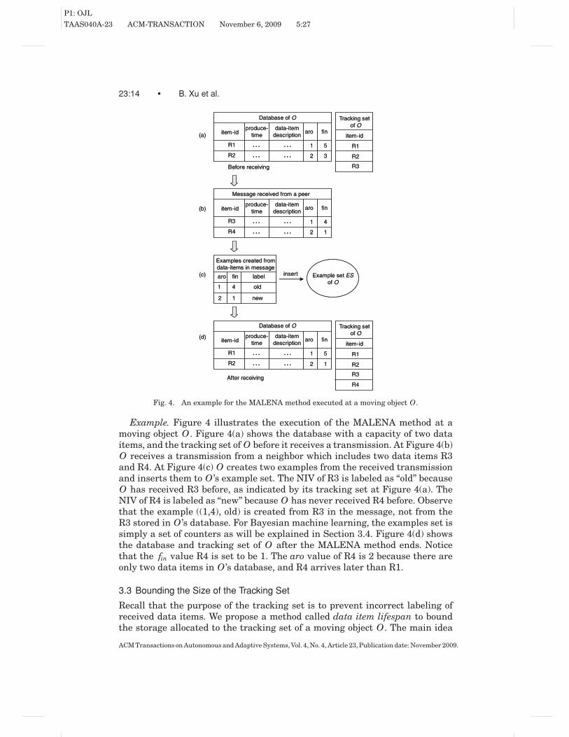
Fig. 4. An example for the MALENA method executed at a moving object O.

Example. Figure 4 illustrates the execution of the MALENA method at amoving object O. Figure 4(a) shows the database with a capacity of two dataitems, and the tracking set of O before it receives a transmission. At Figure 4(b)O receives a transmission from a neighbor which includes two data items R3and R4. At Figure 4(c) O creates two examples from the received transmissionand inserts them to O ’s example set. The NIV of R3 is labeled as “old” becauseO has received R3 before, as indicated by its tracking set at Figure 4(a). TheNIV of R4 is labeled as “new” because O has never received R4 before. Observethat the example ((1,4), old) is created from R3 in the message, not from theR3 stored in O ’s database. For Bayesian machine learning, the examples set issimply a set of counters as will be explained in Section 3.4. Figure 4(d) showsthe database and tracking set of O after the MALENA method ends. Noticethat the fin value R4 is set to be 1. The aro value of R4 is 2 because there areonly two data items in O ’s database, and R4 arrives later than R1.

3.3 Bounding the Size of the Tracking Set

Recall that the purpose of the tracking set is to prevent incorrect labeling ofreceived data items. We propose a method called data item lifespan to boundthe storage allocated to the tracking set of a moving object O. The main idea


P1: OJL



is that O removes a data item R from the tracking set when the lifespan ofR ends, that is, when R has been purged by all the moving objects from theirdatabase. Intuitively, if R has already been purged by all the moving objectsfrom their database, then R will not be received again, so there is no risk ofincorrect labeling. Thus, in this case there is no reason to keep the trackinginformation for R. Obviously the lifespan of R is not known by an individualmoving object O, but intuitively, O assumes that the lifespan of R ended whenO has not received R from other moving objects for a sufficiently long time.More precisely, the lifespan of R is estimated based on the history of R in O ’sown database plus an extension period. Specifically, each entry R of the trackingset contains an element called the expiration time. The expiration time is O ’sestimate of R ’s lifespan. When the expiration time of R arrives, R is removedfrom the tracking set. The expiration time is updated as follows. When an entryR is added to the tracking set, its expiration time is initialized to be infinite.When R is purged from O ’s database, say at time now, the expiration timeof R is updated to be R ’s-produce-time + (now-R ’s-produce-time) * 2. Recallthat produce time is the time at which R is produced (see Section 2.1). In otherwords, the lifespan of R is initially estimated to be: (the period of time startingwhen R is produced and ending when R is purged from O ’s database) * 2. Thatis to say, the global lifespan of R is estimated to be twice the lifespan of Robserved locally at O. Each time R is received again, if R is still in the trackingset, then the expiration time of R is updated in the same fashion. Namely theexpiration time of R is updated to be R ’s-produce-time + (now−R ’s-produce-time) * 2, where now is the time at which R is received again. (Observe thatR is not going to be saved by O in the database according to step 7 of theMALENA method.) In other words, the lifetime of R is estimated to be twice theperiod of time starting when R is produced, and ending when R is last receivedby O.

There is one issue with the data item lifespan method: the clocks amongthe moving objects may be asynchronous, and the clock differences affect thecalculation of the lifespan. This issue can be solved as follows. When two movingobjects A and B exchange data items, they exchange their clocks as well. Foreach new report R received at A from B, A adjusts the produce-time of R usingthe difference between A’s clock and B’s clock. Thus the produce-time of R isgiven in terms of the local clock, and the clock difference does not affect thecalculation of the lifespan of R at A.

The size of the tracking set can also be bounded by another method, calledglobal-DB-size. With global-DB-size, a moving object keeps the tracking in-formation for only the N ·M most recently received data items, where N isthe number of moving objects in the system, and M is the average databasesize among these objects. We postulate that having the size of the trackingset bounded by N ·M should work almost as well as the infinite tracking set,because N ·M gives the maximum number of distinct data items that can cur-rently exist in the system. This postulate has been verified by our preliminaryexperiments. Experiments show that the global-DB-size method and the dataitem lifetime method provide identical performance but the latter bounds thetracking set to a smaller size.


P1: OJL


23:16 • B. Xu et al.

3.4 Bayesian Learning System

In this subsection we introduce the Bayesian system as an instantiation of themachine learning system Q used by the MALENA method. The system can beplugged into the MALENA method for training (step 6) and data items ranking(steps 2 and 7).

At a high level, the Bayesian learning system maintains a set of counters(e.g., the number of “new-data item” examples with a particular (aro, fin) pair).When an example is added, these counters are updated. When invoked forranking, the system uses these counters to compute the probability that a dataitem will be new to a moving object encountered in the future.

Now we describe the Bayesian learning system in further detail. The de-scription focuses on the case where the NIV consists of only two indicators,(aro, fin), because our experiments have shown that adding more indicators willnot change the performance significantly; and on the other hand it increasesresource consumption, and complicates learning significantly.

The probability that a data item is new given its NIV (aro, fin) is

p(new|(aro, fin)) = Cnew(aro, fin)C(aro, fin)

, (1)

where C(aro, fin) is the number of examples for which the NIV equals to (age, fin)and Cnew(aro, fin) is the number of “new-data item” examples for which the NIVequals to (aro, fin).

The novelty probability of a data item with NIV (age, fin) is then taken to bep(new|age, fin) which is computed according to Eq. (1).

Given an example ((aro, fin), label), the INSERT EXAMPLE procedure in-creases C(aro, fin) by 1; and if the label of the example is “new”, then Cnew(aro,fin) is also increased by 1. Thus, assuming that the counters of an (aro, fin)pair are accessed using a hash table, the time complexity of the procedure isconstant.

4. PERFORMANCE OF MALENA

In this section we report on the comparison of MALENA with three other datadissemination methods. In Section 4.1 we introduce the other methods, in Sec-tion 4.2 we describe the simulation method and data used; we also discuss theoverhead of MALENA compared to the alternatives. In Section 4.3 we defineand discuss the performance measure by which the methods are compared, andin Section 4.4 we report and discuss the comparison results.

4.1 The Methods Compared

In this subsection we compare the MALENA method introduced in Section 3,and three other naı̈ve methods. One naı̈ve method determines the noveltyprobability based on aro alone, and one determines the novelty probabilitybased on fin alone. They are called aro-ranking and fin-ranking, and are simi-lar to MALENA, except that no machine learning is used, and each one is basedon a single indicator.


P1: OJL



In aro-ranking, in an encounter, the data items are sorted in decreasing orderof arrival, and the top-k, that is, the k items that arrived latest are exchanged.When saving the received data items in the database, if there is not enoughspace available, the bottom-k data items are discarded.

In fin-ranking the data items are sorted in increasing order of fin values,and the top-k, that is, the k items that have been received the least times areexchanged. When saving the received data items in the database, if there is notenough space available, the bottom-k data items are discarded.

The third naı̈ve method is the random-spread mode of PeopleNet [Motaniet al. 2005], in which data items are randomly selected for saving andtransmission.

We compare the methods in two application scenarios. One is dissemination,in which a data item is to be delivered to as many moving objects as possible.Another scenario is routing, in which a data item is to be delivered to a singledestination.

4.2 Simulation Method

In this section we discuss various components of the simulation system. InSection 4.2.1 we discuss the mobility and communication model, as well as theinput data used for the simulation. In Section 4.2.2 we discuss the databasesize. Since we gave the other methods extra storage to account for the over-head of MALENA, this overhead is discussed in Section 4.2.2. Furthermore,the computational and energy overhead are also discussed there. In Sections4.2.3 and 4.2.4 we discuss moving objects turnover and data items generation,respectively.

4.2.1 Mobility and Communication. We built a simulation system usingJava. For mobility and communication, we used the trace collected by the Com-puter Laboratory at Cambridge University (see Hui et al. [2005]) at the IEEEInfoCom 2005 conference in Miami. This trace records the Bluetooth encoun-ters by small devices, called iMotes, which were carried by 41 attendees (movingobjects) in the conference for 3 days. The record for each encounter contains theIDs of the pair of moving objects involved in the encounter and the time inter-val during which they stay in contact (i.e., the contact interval). Within eachcontact interval the two objects are able to communicate using Bluetooth. Weused the records of the second day for the time period from 8am to 4pm. Duringthis time, on average each iMote experienced an encounter every 130 seconds,and the average contact interval lasts for 160 seconds; each iMote has an aver-age of 1.2 neighbors at a point in time.

We superimposed data items exchanges over the iMotes trace as follows.At each second of a contact interval, the pair of encountering moving objectsexchange their database (the reason for multiple exchanges during a contactinterval is to disseminate to the neighbor new data items received or producedsince the last exchange). For each exchange, a moving object A transmits afraction q of its database to its peer B and vice versa. The communication isassumed to be reliable in the sense that there are no errors and retransmissions,and the simulation results were obtained in this context. In Section 4.4.5 we


P1: OJL


23:18 • B. Xu et al.

study the case in which the communication is not reliable. The parameter q isused to model the constraints imposed by the bandwidth/energy allocation. Asmall q simulates a situation in which the power allocated by the user to P2Pdissemination is low. So, the user assigns to mobile P2P a memory allocation(which may vary from one user to the next, that is, from one moving object tothe next) and a fraction q of this allocation which bounds the transmission ineach encounter. In our simulations q is the same for all the moving objects inone experiment but it may vary for different experiments.

One limitation of the iMotes trace is that it does not record the physical lo-cations (x-y coordinates in a geospace) of the moving objects. This prevents oursimulation system from using a network simulator such as ns-2 [ISI 2009] toincorporate the intricate details of the Bluetooth protocol. In such a simulator,physical locations have to be known for determining the operation of the net-work. As a result, our simulation system does not capture the communicationfactors such as radio attenuation, wireless collisions, and the resulting packetlosses. However, remember that the focus of the article is data item prioriti-zation (that can be combined with any store-and-forward data disseminationalgorithm, and in particular any collision management mechanism), thus ignor-ing collisions should not affect the comparison among various ranking methods.

We also conducted simulations using a synthetic mobility model called Ran-dom Way-Point (RWP). The purpose is to evaluate the methods in a 802.11-like environment where the transmission range, 100 meters (see e.g., GigaFast[2009]), is much higher than in a Bluetooth environment. In the RWP simula-tions on average each moving object has 18 neighbors. The results are betterthan those obtained from the iMotes trace, but due to space considerations weneed to omit most of these. Unless specified, the simulation setup and resultspresented in this section pertain to the iMotes trace.

4.2.2 Database Size and the Overhead of MALENA . The size of each dataitem is 3000 bytes. The number of data items that fit in the database of eachmoving object is randomly chosen from [.5×M , 1.5×M ], where M is fixed tobe 100. In order for the comparison to be fair, in the simulations of PeopleNet,aro-ranking, and fin-ranking methods, we expanded the database size of eachmoving object to match the space overhead of MALENA.

The space overhead of MALENA consists of three components. The first com-ponent is the NIV’s attached to each data item in the database. The size of eachNIV is 2 bytes (1 byte aro value and 1 byte fin value). Thus the space over-head of the NIV’s is 2·M = 200 bytes. The second component is the trackingset. We examined both the global-DB-size method and the data item lifespanmethod for bounding the size of the tracking set (see Section 3.3). It turnedout that data item lifespan is strictly superior to global-DB-size in the sensethat the former provides as good flooding performance as the latter but resultsin a smaller tracking set size. Using the global-DB-size method, we limit thesize of the tracking set to be N ·M , where N is the number of moving objectsin the system, that is, 41. Each entry of the tracking set is a 4 byte item-id.Thus the space overhead of the tracking set is 4·N ·M = 16,400 bytes. We usethe size of the global-DB-size (i.e., 16,400 bytes) to count the space overhead


P1: OJL



Table I. System Parameters and Their Values

Parameter Symbol Unit ValueMean of database size M data item 100 (In section 4.4.4 the database

size varies. See details there)Data item size byte 3000 (In section 4.4.4 the data item

size varies. See details there)Data item production rate f items/second 0.5, 2Delivery-time bound c minute 0, 1, 2, . . . , 60Transmission fraction q 0.02, 0.1Turn-over rate Low: no turn-over

High: normal distribution (300, 300) seconds for lifespanInjection percentage High: normal distribution (80%, 0%)

Low: injected to a single random object

of MALENA even when the data item lifespan method is used. This clearlyfavors the other compared methods. The third component is the storage of theBayesian counters (i.e., C(aro, fin)’s and Cnew(aro, fin)’s). The size of this storagestraightly depends on the number of distinct (aro, fin) pairs that are receivedby a moving object. Specifically, let Mmax be 1.5 × M = 150, that is, the max-imum size aro in the system. Let Wmax be the maximum fin value that maybe received by an object. In our simulations Wmax is 15. Then the maximumnumber of the C(aro, fin) counters (or Cnew(aro, fin)) is Mmax · Wmax . The sizeof each counter is 2 bytes. Thus the space overhead of the Bayesian counters is4 ·Mmax · Wmax = 9, 000 bytes. Thus we increased the database size by 9 dataitems for PeopleNet, aro-ranking, and fin-ranking.

The communication overhead of MALENA results from the NIV’s attachedto the transmitted data items. The size of each NIV is 2 bytes, and there-fore the communication overhead of MALENA is 2·M · q bytes (see Table Ifor symbol interpretation) per transmission, or at most 20

3000 data items for a3000-byte data item. We consider this overhead negligible for this data itemsize.

Finally, let us discuss the computational overhead of the MALENA method.It consists of two components. The first component is ranking in steps 2 and7 of the method (see Section 3.2). Ranking of 100 keys takes at most 15,000instructions, thus this component takes 30K instructions. The second compo-nent is the computational cost for maintaining the tracking set (which takesabout 10 instructions per data item when the tracking set is accessed usinga hash-table), and the cost of the INSERT EXAMPLE procedure (which againtakes about 10 instructions per data item when a hash-table is used to access acounter). Thus, the overhead of the second component is at most 2000 instruc-tions, and overall the computational overhead of MALENA is less than 32Kinstructions per data items exchange.

Now we estimate the time and the energy consumed by the MALENA compu-tation. We consider a typical PDA system, namely Dell X50 with a 624 MHz IntelPXA270 processor and a 1100 mAh, 3.7V Li-ion battery. Assuming that the CPUprocesses one instruction per clock cycle, each instruction takes 1/(624×106) sec-ond. Thus 32K instructions take less than 50 μs. In other words, each executionof the MALENA computation takes less than 50 μs.


P1: OJL


23:20 • B. Xu et al.

Now consider the total energy consumed by the MALENA computation ata moving object throughout an 8-hour period. Since each moving object hasone exchange with each one of its neighbors per second, and on average eachmoving object has 1.2 neighbors (see Section 4.2.1), each moving object has1.2×28800 exchanges during the 8 hours. The CPU consumption is at most5.3Watt [Dell 2009]. Thus the total energy consumed by the MALENA compu-tation is at most 50 × 10−6 × 1.2 × 28800 × 5.3 = 9 Joules, that is, 0.06% ofthe total battery capacity (3.7 × 1.1 × 3600 = 14652 Joules). It is noted thatthe preceding calculation considers only the energy overhead introduced by theMALENA method (for machine learning and ranking). It does not include theoverhead of the gossiping protocol itself, such as the communication energy, thedevice and service discovery energy, and the extra energy costs of waking up asleeping kernel. Presumably, these energy costs are incurred by any gossipingprotocol.

4.2.3 Moving Objects Turnover. Each moving object has a lifespan deter-mined by the simulation system. When the lifespan of an object O expires, itsdatabase, tracking set, and Bayesian counters are reinitialized. This simulatesO exiting the system and a new object entering it. Thus the number of livemoving objects is fixed during a simulation run.

We consider two cases in terms of the lifespan. In the first case, the lifespanof each object equals to the length of the time period of the whole simulationrun. This case is referred to as low turnover as it represents an environmentin which the set of moving objects is fixed, that is, no new objects join in thesystem and no existing objects leave. Places such as conference halls or sportsstadiums are practical examples of low turnover environments. In the secondcase, the lifespan of each object follows a normal distribution with the mean of300 seconds and the standard deviation of 300 seconds. This case is referred toas high turnover as it represents an environment in which objects frequentlyjoin in and exit. Places such as train stations and airport terminals are examplesof high turnover environments.

4.2.4 Data Items Injection. In each simulation run f data items are pro-duced every second. The number f is referred to as the data item productionrate. In the routing scenario, a destination for the data item is generated to-gether with the item. The destination of a data item is randomly chosen fromthe objects that have ever entered the system and the objects that will enter thesystem in the future. When produced, the data item is injected instantaneouslyto a percentage of moving objects which become its producers. We consider twocases. In the first case, the data item is injected to a single moving object whichis randomly selected. This is referred to as the low injection case. It simulates,for example, a matchmaking profile being generated by a single user. In thesecond case, the percentage of moving objects that learn the data item follows anormal distribution with the mean of 80% and the standard deviation of 20%.This is referred to as high injection case. An example of a high injection casewould be where some users subscribe for stock quotes notifications or news


P1: OJL



alerts via the cellular network and then they share the information with otherusers via peer-to-peer data dissemination.

All the system parameters and their values are listed in Table I. Each pa-rameter configuration is run once to get the curve for that configuration.

Now let us justify that our communication setup is reasonable in the sensethat the bandwidth consumed by pairwise exchanges fits within the capacityof Bluetooth. In our experiments, each moving object exchanges with each ofits neighbors at each second, each exchange is finished within 1 second, andon average each moving object has 1.2 neighbors at any point in time. Sincethe maximum database size is 150 and the transmission fraction is at most0.1, each moving object communicates (transmitting and receiving) at most3000bytes/item × 150items × 0.1 × 1.2 ×2 = 108 Kbytes = 864Kbits per second,well within Bluetooth’s theoretical bandwidth limits. In other words, the wholedatabase can be transmitted within one second. And indeed all the iMotescontact intervals are at least one second. In addition, in the iMotes traces, eachcontact interval must have excluded the device discovery time and the servicediscovery time because the contact interval started after the device and theservice are discovered.

4.3 Performance Measure

As the performance measure for comparison of the four methods we take acombination of throughput and delivery-time; it averages the number of dis-tinct data items received by a moving object within a certain time limit c. Thisis similar to the way an academic department is evaluated according to thepercentage of its students that graduate within 4 years.

More specifically, the measure takes the average number of data items withdelivery-times smaller than c that are successfully delivered to a moving ob-ject. In the routing scenario, only those data items those are addressed toand received by the destination object are counted. This measure is called thedelivery-time bounded throughput, or throughput, and c is called the delivery-time bound. By varying the value of c, we evaluate the throughput of a methodfor different delivery-time constraints.

Finally we define the delivery-time of a data item R received at a movingobject O. Intuitively, the delivery-time interval starts at the time at which O isintroduced in the system or R is introduced, whichever is later, since both mustbe present for O to receive R. The interval ends when O receives R. Formally,let O receive a data item R for the first time at time t. If R is produced afterO is introduced in the system, then the delivery-time is the length of the timeperiod starting at the production-time of R and ending at time t; otherwise itis the length of the time period starting at the time O is introduced and endingat time t. This concept is illustrated by Figure 5.

Observe that it is possible to evaluate performance by other measures, suchas the probability that a data item is disseminated to all the moving objectsin the system, but we chose the more traditional throughput and delivery-timemeasures.


P1: OJL


23:22 • B. Xu et al.

R1

A

t1 tA t2t1A time

delivery-time

of R1delivery-time of R2

R2

t2A

A receives R1

A receives R2

R1R1

AA

t1 tA t2t1A time

delivery-time

of R1delivery-time of R2

R2R2

t2A

A receives R1

A receives R2

Fig. 5. Illustration of delivery-time calculation. Data items R1 and R2 are produced at times t1and t2 respectively. Object A is introduced at time tA. The delivery-time of R1 is t1A − tA. Thedelivery-time of R2 is t2A−t2.

0

2000

4000

6000

8000

10000

12000

14000

0 5 10 15 20 25 30 35 40 45 50 55 60

thro

ug

hp

ut

(dat

a-it

ems/

ob

ject

)

delivery-time bound (minute)

low-turn-over/low-injection, Bluetooth, M=100, f=2, q=0.1, dissemination

MALENAaro-rankingfin-rankingPeopleNet

Fig. 6. Experiment 1: L/L environment for the Bluetooth scenario.

4.4 Simulation Results

In this section we discuss the results in the dissemination scenario. In Sections4.4.1 and 4.4.2 we compare the four ranking methods in a low-turnover/low-injection environment and a high-turnover/high-injection environment, respec-tively. In Sections 4.4.3 and 4.4.4 we study the impact of transmission fractionand data item size, respectively. We evaluate the impact of the communicationreliability in Appendix B. The results for the routing scenario are similar, thusthey are omitted. The results presented in Figures 6, 7, and 8 were obtainedusing the data item lifespan tracking set bounding method. The results in allthe other figures were obtained using the global-DB-size method.

4.4.1 Low-Turnover/Low-Injection (L/L) Environment. Experiment 1(Figure 6) shows the throughput as a function of the delivery-time bound fordifferent methods in the L/L environment for the Bluetooth scenario. Observethat aro is a good indicator in the L/L case, as aro-ranking performs at leastthree times better than fin-ranking, for the entire range of the delivery-timebound. MALENA closely follows aro-ranking. Intuitively, in the L/L case, theset of the moving objects in the system is fixed, and therefore a data item thathas stayed at a moving object for a long time is likely to be known by manyobjects.

Observe that with MALENA, each moving object receives about 11,000 newdata items with delivery-times 60 minutes or less. On the other hand, two dataitems are generated per second in the whole system. Thus, the performance of


P1: OJL



0

5000

10000

15000

20000

25000

30000

0 1 2 3 4 5th

rou

gh

pu

t (d

ata-

item

s/o

bje

ct)


low-turn-over/low-injection, 802.11, M=10, f=1, q=1, dissemination


Fig. 7. Experiment 2: L/L environment for the 802.11 scenario.

0 20 40 60 80

100 120 140 160 180 200

0 5 10 15 20 25 30 35 40 45 50 55 60

thro

ug

hp

ut

(dat

a-it

ems/

ob

ject

)


high-turn-over/high-injection, Bluetooth, M=100, f=2, q=0.1, dissemination


Fig. 8. Experiment 3: H/H environment for the Bluetooth scenario.

MALENA is 20% of the ideal case (i.e., when a central server is employed, andit instantaneously broadcasts each new data item to all the moving objects; inthis case a moving object would have received 57600 data items). In addition,75% of the data items received by MALENA are younger than 5 minutes, wellwithin reasonable limits for the applications considered.

Experiment 2 (Figure 7) shows the results with the Random Way-Point(RWP) mobility model with 802.11 in the L/L case (Recall that with 802.11each moving object has 18 neighbors on average, in contrast to 1.2 for the Blue-tooth case). The comparison among the methods is similar to that with theiMotes trace (Bluetooth) except that MALENA performs even better.

4.4.2 High-Turnover/High-Injection (H/H) Environment. Experiment 3(Figure 8) shows the throughput as a function of the delivery-time bound forthe different methods in the H/H environment. Observe that fin is a good indi-cator in the H/H case, as it performs much better than aro-ranking (by up to30%). MALENA is almost as good as fin-ranking. The fact that the aro indicatorperforms poorly can be explained as follows. Since the turnover rate is high,even the old data items are “new” to the moving objects that have newly joinedin. On the other hand, since the injection percentage is high, “young” data itemsare known to the moving objects that have been injected with them. Thus, arobecomes a bad indicator of novelty.


P1: OJL


23:24 • B. Xu et al.

0

2000

4000

6000

8000

10000

12000

0 5 10 15 20 25 30 35 40 45 50 55 60th

rou

gh

pu

t (d

ata-

item

s/o

bje

ct)


low-turn-over/low-injection Bluetooth, M=100, f=2, q=0.02, dissemination


Fig. 9. Experiment 4: Low transmission fraction in the L/L environment for the Bluetooth scenario.

In terms of the delivery-time, observe that 95% of all the data items receivedby MALENA are younger than 5 minutes.

4.4.3 Impact of the Transmission Fraction. Experiment 4 (Figure 9) dif-fers from Experiment 1 (Figure 6) in the value of the transmission fraction (q).Specifically, in Experiment 1 on average ten data items are exchanged per en-counter, whereas in Experiment 4 two data items are exchanged per encounter.It can be seen that the advantage of MALENA over PeopleNet is higher whenthe transmission fraction is lower. This suggests that MALENA is particularlyuseful in an environment where the available bandwidth and power are low.Intuitively, when the transmission fraction is low, the prioritization becomesmore critical and random ranking suffers. The same can be observed in theH/H environment.

4.4.4 Impact of the Data Item Size. In all the previous simulations, the sizeof each data item is fixed to be 3000 bytes. In this subsection we vary the dataitem size and study its impact to the performance of the ranking methods. Firstlet us discuss how we take the space and communication overhead of MALENAinto account in the simulations conducted in this subsection. We fix the size ofthe database of MALENA to be 300K bytes. The space overhead of MALENAis taken into account as described in Section 4.2.2, with M fixed to be 300K/L;L is the data item size (excluding NIV).

The communication overhead of MALENA is taken into account as follows.Denote the cardinality of a transmission set by k. For the MALENA method,k = 300K·q/L. Since each transmitted data item is attached with a 2 byte NIV,the communication overhead of MALENA is 2·k bytes per transmission, or2·k/L data items. For aro-ranking, fin-ranking, and PeopleNet, k is increasedto compensate the communication overhead of MALENA. The increase is asfollows. When 2·k/L is greater than 1, k is increased by 2 · k/L data items.When 2·k/L is smaller than 1, for each transmission, k is increased by 1 withprobability 2·k/L.

Experiment 5 (Figure 10) corresponds to Experiment 1 in terms ofparameters-configuration, and shows the throughput as a function of the dataitem size for the four methods in the Bluetooth L/L environment. The delivery-time bound is fixed to be 900 seconds since the throughput of each method


P1: OJL



0

5000

10000

15000

20000

25000

3000 2500 2000 1500 1000 500 250th

rou

gh

pu

t (d

ata-

item

s/o

bje

ct)

data-item size (byte)

low-turn-over/low-injection Bluetooth, database size=300K bytes, f=2, q=0.1, dissemination, delivery-time bound=900 seconds


Fig. 10. Experiment 5: Impact of the data item size. L/L environment for the Bluetooth scenario.

except fin is stable beyond this bound. From Experiment 5 it can be seen that,as the data item size decreases, the throughput increases for all the methods.Furthermore, the advantage of MALENA over fin decreases as the data itemsize decreases. This suggests that in a L/L environment, MALENA is particu-larly useful when the data item size is big.

However, the difference between MALENA and aro or PeopleNet does notchange much with data item size. This is because the communication overheadof MALENA remains very small even when the data item size is small. Infact, MALENA only adds two bytes to each transmitted data item. Thus evenwhen the data item is 250 bytes (the smallest size tested), the communicationoverhead of MALENA is only 2/250 = 0.8%.

Summary. In each environment MALENA comes close or exceeds the bestindicator for that environment. This is important since a moving object usuallydoes not know the parameters of its current environment, and furthermore,they change over time.

5. NOVELTY RANKING IN PUSH-PULL GOSSIPING

In this section we study novelty ranking in another gossiping protocol, calledpush-pull gossiping. Let W be the maximum number of bytes that can betransmitted by a moving object O at each exchange, according to the band-width/energy allocation. W is called the communication bound, and it is com-puted based on the database size at O, the data item size, and the transmissionfraction, q. When O encounters a moving object A, a push-pull gossiping is ex-ecuted as follows.

(1) O informs A what are the ids of the data items that O has ever seen. Thisis done by O sending its tracking set (denoted TSO ) to A.

(2) Symmetrically O receives TSA the tracking set of A.(3) O transmits to A the data items that are new to A, that is, those data items

whose ids do not appear in TSA. If all the data items that are new to A donot fit the remaining transmission size (the remaining transmission size isW−size(TSO ), where size(TSO ) is the size of TSO in number of bytes), then


P1: OJL


23:26 • B. Xu et al.

the data items are ranked according to their novelty probabilities and thetop ones that fit in W−size(TSO ) bytes are transmitted to A.

(4) Symmetrically O receives data items from A. O ranks the data items re-ceived from A together with the data items in the database, and saves thetop MO data items in the database.

The rest of this section is organized as follows. In Section 5.1 we intro-duce MALENA+2P, the push-pull version of MALENA. In Section 5.2 we com-pare MALENA+2P and the push-pull versions of aro-ranking, fin-ranking, andPeopleNet. We compare MALENA+2P with the push version of MALENA inAppendix C.

5.1 MALENA+2P: The Push-Pull Version of MALENA

First, observe that MALENA does not attempt to estimate the probability ofnovelty to the peer participating in the current encounter, but to a future en-countered peer. Thus, the fact that the push-pull gossiping transmits only newdata items does not obviate the need for estimating novelty probability.

Second, observe that MALENA could be applied to the push-pull gossipingwithout any changes. In other words, a moving object O creates examples andtrains the machine learning system Q (see Section 3.2) when O receives dataitems from a peer A (after O informs A of its tracking set). However, thereis a drawback to this straight forward carry-over. Since A only transmits newdata items to O, all the examples created by O will be labeled as “new.” ThusQ will be trained with only positive examples, instead of with both positiveand negative examples as in the push case. This may compromise the learningcapability of Q . In some cases it simply fails the machine learning system. Forexample, the Bayesian method used in this article does not work when thereare only positive examples.

In this subsection we adjust MALENA such that it learns from both positiveand negative examples in the push-pull gossiping. The idea is that, insteadof O learning upon receiving data items from A, it learns upon receiving thetracking set of A. Specifically, for each data item R in O ’s database, one exampleis created using the NIV of R: the example is labeled as “new” if R is new to A(i.e., the id of R does not appear in A’s tracking set); and “old” otherwise. Wecall this method MALENA+2P and formally describe it next.

Similar to the MALENA method, the complexity of MALENA+2P isO(MlogM), where M is the number of data items in the database.

Let us explain step 3, where the method increases the fin value by 1 for eachdata item in O ’s database that is known by A. Observe that in the push-pullgossiping, since a peer only transmits new data items to O, O will not receive adata item R more than once. Thus the original definition of fin (i.e., the numberof times R is received) will give at most 1 for the value of fin, regardless of howmany peers encountered by O have known R before the encounters. This clearlydeviates from the purpose of the fin as a novelty indicator. In the MALENA+2Pwe address this issue by redefining fin to be the number of times O has sightedR ’s item-id in the tracking sets of the peers it has encountered. In step 3, themethod increases the fin value of R by one if it sights R in the tracking set of A.


P1: OJL



Algorithm 2. The MALENA+2P method, executed at a moving object O, when O en-counters another moving object A.

1. Receive from A the tracking set TSA of A.2. For each data item R in O ’s database and its NIV X,

a. Create an example (X, label) where label is “new” if the item-id of R appears inTSA, and “old” otherwise.

b. Invoke INSERT EXAMPLE((X, label)) to add the example (X, label) to theexamples set.

c. If the item-id of R does not appear in TSA, mark R as “candidates fortransmission”.

3. For each item-id i in TSA, if i appears in the database of O, then update the NIV ofi (in O ’s database) by increasing its f in value by 1.

4. For each data item R marked as “candidates for transmission”, compute the noveltyprobability using the machine learning system denoted Q . Then sort these data-items in decreasing order based on their novelty probabilities, and select the topk data items (i.e., k items with highest probabilities); the value of k is determinedby the data-item size and the remaining transmission size (recall that the remainingtransmission size is the communication bound W minus the size of O ’s tracking set).

5. Transmit the selected data-items to A6. Transmit the tracking set of O to A and receive a set of data items from A. All the

received data items have the same aro, denoted arom, where arom = 1+ (the currentmaximum aro in O ’s database). All the received data-items have fin = 1.

7. For each data-item R received from A, insert R ’s-item-id to the tracking set.8. Sort the data items received from A in step 6 together with the data items in the

database, in decreasing order of their novelty probabilities (computed by the machinelearning system Q); save the top MO data items in the database.

9. The aro values of the remaining data items are adjusted to start from 1 and toeliminate the gaps created by the data-items that did not fit in the database.

5.2 Comparison of MALENA+2P and the Push-Pull Versions of aro-ranking,fin-ranking, and PeopleNet.

We conducted simulations to compare MALENA+2P, fin-ranking+2P, aro-ranking+2P, and PeopleNet+2P where fin-ranking+2P, aro-ranking+2P, andPeopleNet+2P are the push-pull versions of fin-ranking, aro-ranking, and Peo-pleNet, respectively. For fin-ranking+2P, fin is defined to be the number oftimes a moving object has sighted the item-id in the received tracking sets (seeSection 5.1). The simulation setup is similar to that for the push gossiping (seeSection 4.2). In Figures 11 and 12 we present the results.

Experiment 12 (Figure 11) shows the results in the low-turnover/low-injection (L/L) case for one parameter configuration (the results with otherparameter configurations point to similar conclusions and are omitted due tospace considerations). Experiment 13 (Figure 12) corresponds to Experiment 3in the push case in terms of parameters configuration, and shows the resultsin the high-turnover/high-injection (H/H) case. From these experiments it can


P1: OJL


23:28 • B. Xu et al.

0

1000

2000

3000

4000

5000

6000

7000

8000

9000

0 5 10 15 20 25 30 35 40 45 50 55 60th

rou

gh

pu

t (d

ata-

item

s/o

bje

ct)


low-turn-over/low-injection Bluetooth, M=10, f=2, q=1, dissemination

MALENA+2Paro-ranking+2Pfin-ranking+2PPeopleNet+2P

Fig. 11. Experiment 12: L/L environment for the Bluetooth scenario.

0

50

100

150

200

0 5 10 15 20 25 30 35 40 45 50 55 60

thro

ug

hp

ut

(dat

a-it

ems/

ob

ject

)


high-turn-over/high-injection Bluetooth, M=100, f=2, q=0.1, dissemination

MALENA+2Paro-ranking+2Pfin-ranking+2PPeopleNet+2P

Fig. 12. Experiment 13: H/H environment for the Bluetooth scenario. (Note that the curve offin-ranking+2P and that of PeopleNet+2P coincide).

be seen that, again, in each individual environment MALENA+2P approachesor outperforms the best one.

6. RELATED WORK

Static-sensor databases. A database approach has been applied to static sensornetworks (see e.g., Yao and Gehrke [2003], Hellerstein et al. [2003], Muller andAlonso [2006], Lian et al. [2005], Coman et al. [2005], Deligiannakis [2004],Xu et al. [2005], and Kotidis [2005]). All these methods require that a cer-tain routing structure, for example, a tree, be established in the network.Each node aggregates the results returned by its downstream neighbors andits own result, and forwards the aggregation result to its upstream neigh-bor. However, in our environment, due to the dynamic/partitionable networktopology, such a structure is hard to maintain. MALENA relies on opportunis-tic interactions between encountering mobile nodes and thus is disruptiontolerant.

Some works in static sensor networks involve negotiations between neigh-boring sensors (see e.g., Medidi et al. [2005]). The objective is to ensure that thedata items wanted (i.e., unknown data items in our context) by the receiver aretransmitted. However, the negotiation considers only what items are new to thereceiver, whereas we consider what are likely to be new data items to futureencountered moving objects. In other words, we consider the utility to moving


P1: OJL



objects functioning as brokers, not consumers. In this article we assume thatthe consumer function of devices is handled orthogonally and independently ofthe broker function.

Novelty ranking. Previous work on dissemination in mobile ad hoc networksand routing in disruption-tolerant networks has studied various heuristics forranking packets based on their novelty probability. For example, Ni et al. [1999]propose two schemes, one using the number of times a packet has been re-ceived at a node (i.e., fin), and another using the distance between the senderand the receiver. Hayashi et al. [2003] and Burges et al. [2006] consider thenumber of hops. Vahdat et al. [2000], Costa et al. [2004], and Chaintreauet al. [2006] use FIFO (equivalent to arrival order). Thus, in each of theseschemes, a single individual novelty indicator is used. In contrast, our methodcombines various indicators and it adapts to the environment via machinelearning.

In Burges et al. [2006], a node uses acknowledgements from destinationnodes to purge from its buffer those packets that have already been receivedby their destinations. This method is designed for DTNs, that is, environmentsin which a message is sent to a specific destination; but it does not work fordissemination where the destination ids are not known a priori to the sender.Our method is applicable for both cases.

Prioritization in mobile peer-to-peer data dissemination. Ranking data itemsfor memory (cache) management and bandwidth management in mobile peer-to-peer networks has been studied in a number of works. In Motani et al. [2005]and Wolfson et al. [2006a; 2006b] data items are ranked according to theirpopularity and the assessment of popularity is enabled via the disseminationof queries. In Wolfson et al. [2007] the rank of a data item is jointly determinedby its popularity and size. In Sailhan and Issarny [2002] the rank of a dataitem is jointly determined by its popularity, reliability, and size. In Xu et al.[2004] data items are ranked based on their spatio-temporal relevance. Therelevance indicates, for example, the probability that a parking slot reportedby the data item will be still available when the user reaches it. In Perich etal. [2004], Hull et al. [2006], and Datta [2004] data items are ranked basedon an abstract utility function which is to be defined by specific applications.Our present work does not compete with these methods. Instead, it adds anorthogonal consideration, the novelty probability which, as mentioned in theIntroduction, can be combined with other priority metrics.

Resource discovery and publish/subscribe in mobile ad hoc networks. Re-source discovery (e.g., Pucha et al. [2004] and Frank and Karl [2004]) andpublish/subscribe (e.g., Huang and Garcia-Molina [2004] and Zhang and Hu[2005]) in mobile ad hoc networks are often implemented by building a routingstructure for resource information dissemination. Consequently they can be in-efficient, particularly in networks that are prone to frequent topology changesdue to mobility and turnover. In such an environment, either a lot of communi-cation has to be expended to keep the routing structure up to date, or the routingstructure rapidly becomes obsolete and misses many matches. Our method doesnot rely on any routing structures and it adapts to the environment via machinelearning.


P1: OJL


23:30 • B. Xu et al.

Peer-to-peer networks. In current P2P networks (see e.g., Halevy et al. [2004]and Balazinska et al. [2002]), the requester sends a query which is propagatedthrough a specific community (say Napster) and if a match is found, the re-sponse is routed back to the requester. The main difference between static andmobile P2P (sensor) networks is that in the mobile case nodes can communi-cate only when they are in physical proximity, whereas static P2P networks arenot so constrained. This fundamental difference makes most static approachesinapplicable. For example, Michel et al. [2006] also use the novelty concept toreduce duplicate transmissions in a P2P environment. In their case, the ids ofthe data items stored at each peer O are summarized by a synopsis. All thesynopses are published to a distributed directory. When another peer P issuesa query, P looks up the synopses and sends the query to the peers that haveminimum overlap in their synopses. This method clearly does not fit a mobileenvironment, due to the overhead of directory maintenance and access, and theconstant change of synopses.

7. CONCLUSION AND FUTURE WORK

In this article we addressed the dissemination problem in which data itemsare flooded to all the moving objects in a mobile ad hoc network. Disseminationoccurs via peer-to-peer communication using short-range wireless networkssuch as 802.11. We first considered the problem in an environment where allthe trajectories of moving objects are known a priori at a centralized location.We showed that if memory and bandwidth are bounded at moving objects, thenthe problem of determining whether a set of data items can be disseminated toall the moving objects is NP-complete; otherwise it is tractable.

We then proposed a method for dissemination of data items based on ma-chine learning. The proposed method, MALENA, is used by each moving objectto prioritize data items in terms of their probabilities of being new to futurerecipients. The machine learning system is progressively trained by receiveddata items.

We experimentally evaluated MALENA using Bayesian as the machinelearning system, and compared it with three other methods. For the gossip-ing protocol we considered both push gossiping and push-pull gossiping. Thesimulation used two inputs, one real and the other synthetic. The real onewas collected as Bluetooth sightings at a convention, and the synthetic onewas generated using the random-way-point modeling an 802.11 network. Themeasure of comparison is new, combining the average number of data itemsreceived by a moving object and their average age when received. The experi-mental results show that in each individual environment MALENA approachesor outperforms the best method for that environment and outperforms the in-ferior one by up to five times. This is important since the best method dependson the global environment, and the global environmental parameters changeand are usually not known to a moving object. The results hold for an applica-tion that has become popular recently, disruption tolerant networks (see Burnset al. [2005]), in which a data item is sent to a single destination rather thandisseminated.


P1: OJL



Much more research still needs to be carried out to determine the optimallearning method for different gossiping protocols. For example, instead of a pair-wise exchange, the moving objects may communicate by periodic broadcasts(see, e.g., Wolfson et al. [2006b]). Does the same learning mechanism workwell in these gossiping protocols? Do other (than Bayesian) machine learningtechniques perform better?

In this article we studied how to transmit during a peer-to-peer interaction.Another important issue is how much to transmit. In other words, if the totalbandwidths of the neighboring moving objects are not sufficient to exchangeall data items, how to allocate bandwidth among these objects? In recent work[Wolfson et al. 2006b; Wolfson and Xu 2007] we addressed this issue. The gen-eral approach is that each moving object dynamically adjusts the transmissionsize based on the length of the period of time between subsequent peer-to-peerinteractions, to deliver reliably (i.e., without collisions) the maximum numberof data items.

In general, there can be many gossiping protocols and they can be comparedin terms of the dissemination performance, the amount of communication, andthe number of rounds of communication. However, developing all these gossip-ing protocols and finding which is the best is clearly out of the scope of thisarticle. In this article we have shown that MALENA improves performance intwo gossiping protocols.

Another important future research issue is to augment MALENA such that itadapts to a changing environment, for example, when an object moves from anL/L environment to an H/H one. In machine learning, changing environmentsare often handled by sliding windows of fixed or adaptive size on the trainingdata (see, e.g., Widmer and Kubat [1996] and Wang et al. [2003]) or by weightingdata or parts of the hypothesis according to their age and/or utility for theprediction task (see, e.g., Taylor et al. [1997]).

APPENDIXES

A. PROOF OF THEOREM 2

THEOREM 2. Given bounds on memory and bandwidth for processors, theMODD problem is NP-complete.

PROOF. The reduction is from the Multiprocessor Scheduling (MS) problem(see Deligiannakis et al. [2004]). Given an instance of MS we create an MODDinstance as follows (the construction uses the Deligiannakis et al. [2004] nota-tion for MS). We introduce a set S of objects, each corresponding to a processorin MS; and a number of data items that is equal to the number of tasks. Themoving objects in S are always within transmission range of each other, andeach has infinite bandwidth. Then we introduce a new moving object s that isnot in S, it is static within the transmission range of all the moving objects inS for the period of time 0 to D (but not afterwards), and it receives all the dataitems at time 0. Due to bandwidth constraints, the time for s to send a dataitem to a member of S is equal to the length of the corresponding task. It is easyto show that the MS instance has a solution if and only if the MODD instancehas a solution.


P1: OJL


23:32 • B. Xu et al.

0

2000

4000

6000

8000

10000

12000

0 5 10 15 20 25 30 35 40 45 50 55 60

thro

ug

hp

ut

(dat

a-it

ems/

ob

ject

)


low-turn-over/low-injection Bluetooth, M=100, f=2, q=0.1, dissemination

MALENA (p=100%)MALENA (p=50%)MALENA (p=30%)MALENA (p=10%)MALENA (p=5%)MALENA (p=1%)

(a) The throughput of MALENA as a function of the delivery-time bound for various communication

reliabilities

0

2000

4000

6000

8000

10000

12000

14000

10050301051

thro

ug

hp

ut

(dat

a-it

ems/

ob

ject

)

communication reliability (%)

low-turn-over/low-injection, Bluetooth, M=100, f=2, q=0.1, dissemination,

delivery-time bound=3600 seconds


(b) The performance of the four methods as a function of the communication reliability (delivery-time

bound=3600 seconds)

Fig. 13. Experiment 11: Impact of the communication reliability. L/L environment for the Blue-tooth scenario.

B. IMPACT OF THE COMMUNICATION RELIABILITY

For all the experiments conducted so far, we assumed that the communicationis perfectly reliable and each exchange always succeeds. In this subsection westudy the case in which the communication is not reliable. Particularly, welet each exchange succeed with probability p. If the exchange does not suc-ceed, no data items are received by either of the two interacting moving ob-jects. p is referred to as the communication reliability. p varies from 1% to100%.

Experiment 11 (Figure 13) shows the impact of the communication relia-bility in the L/L environment for the Bluetooth scenario. Figure 13(a) showsthe throughput of MALENA as a function of the delivery-time bound for var-ious communication reliabilities. Figure 13(b) shows the performance of thefour methods as a function of the communication reliability, with the delivery-time bound fixed to be 3600 seconds. From Figure 13(b) it can be seen that thefour curves are quite flat when the communication reliability is higher 30%.This means that all the four methods are tolerant to communication failures.


P1: OJL



0

1000

2000

3000

4000

5000

6000

7000

8000

500 1000 1500 2000 2500 3000th

rou

gh

pu

t (d

ata-

item

s/o

bje

ct)

data-item size (byte)

low-turn-over/low-injection Bluetooth, database size = 30K bytes, f=2, q=0.1, dissemination, delivery-time bound=600 seconds

MALENAMALENA+2P

Fig. 14. Experiment 14: Comparison of MALENA+2P and MALENA in a L/L environment for theBluetooth scenario.

Particularly, when 50% of the exchanges fail, the throughput of MALENA dropsonly 5%.

C. COMPARISON OF MALENA+2P AND MALENA

Observe that in MALENA+2P, two encountering moving objects exchangetracking sets so that only the new data items are exchanged. In other words,the communication cost of the data item exchange is reduced, but the trackingset exchange is added. Presumably, when the size of each data item is big, thenthe overhead of the tracking set communication is relatively small comparedto the reduction of data item communication, and MALENA+2P is efficient.On the other hand, when the data item size is small, then MALENA+2P maynot be worthwhile. Our simulations results validated this intuition and furtheridentified the cut-off sizes (i.e., the data item sizes beyond which MALENA+2Poutperforms MALENA) for various parameter configurations. Figure 14 showsthroughput as a function of the data item size for MALENA+2P and MALENAin a Bluetooth L/L environment. The delivery-time bound is fixed to be 600seconds since the throughput of either method is stable beyond this bound.

From Experiment 14 (Figure 14) it can be seen that the cut-off size is about600 bytes for the given parameter configuration. Observe that the throughputof MALENA increases as the data item size decreases. This is because witha smaller data item size, more data items can be stored in the database andtransmitted during an exchange. The behavior of MALENA+2P is a little bitmore intricate. The throughput of MALENA+2P increases as the data itemsize decreases from 3000 bytes to 1500 bytes, and then it decreases as thedata item size decreases from 1500 bytes to 400 bytes. This is explained asfollows. When the data item size increases, two effects, positive and negative,are generated. On one hand, more data items can be stored in the database andbe potentially transmitted; on the other hand, the overhead of the tracking setexchange increases because there are more tuples in the tracking set (RecallSection 3.2; the number of entries in the tracking set is proportional to thenumber of tuples in the database). The increase of the tracking set leaves lessroom for the data item exchange. Experiment 14 shows that the data item sizethat optimally trades off these two effects is 1500 bytes.


P1: OJL


23:34 • B. Xu et al.

The cut-off size may vary depending on the environmental parameters suchas the transmission fraction and the data item production rate. For example,for the parameter configuration used in Experiment 14, when the data-timeproduction rate ( f ) is changed from 2 to 10, the cut-off size is changed from600 bytes to 300 bytes. Thus our simulation results enable the moving objectsto decide whether to use MALENA or MALENA+2P in a specific environment.However, remember that whether to use push gossiping or push-pull gossipingis an issue in selecting the dissemination algorithm, whereas the focus of thearticle is the machine learning method which, as we have shown, can improveeither.

REFERENCES

BALAZINSKA, J., BALAKRISHNAN, H., AND KARGER, D. 2002. INS/Twine: A scalable peer-to-peer ar-chitecture for intentional resource discovery. In Proceedings of the International Conference onPervasive Computing. 195–210.

BIRMAN, K., HAYDEN, M., OZKASAP, O., XIAO, Z., BUDIU, M., AND MINSKY, Y. 1999. Bimodal multicast.ACM Trans. Comput. Syst. 17, 2, 41–88.

BURGES, J., GALLAGHER, B., JENSEN, D., AND LEVINE, B. 2006. MaxProp: Routing for vehicle-baseddisruption-tolerant networking. In Proceedings of the 25th IEEE Conference on Computer Com-munications. 1–11.

BURNS, B., BROCK, O., AND LEVINE, B. N. 2005. MV routing and capacity building in disruptiontolerant networks. In Proceedings of IEEE InfoCom. 398–408.

CHAINTREAU, A., HUI, P., CROWCROFT, J., DIOT, C., GASS, R. AND SCOTT, J. 2006. Impact of humanmobility on the design of opportunistic forwarding algorithms. In Proceedings of the 25th IEEEConference on Computer Communications. 1–13.

COSTA, P., MIGLIAVACCA, M., PICCO, G., AND CUGOLA, G. 2004. Epidemic algorithms for reliablecontent-based publish-subscribe: An evaluation. In Proceedings of the 24th IEEE InternationalConference on Distributed Computing Systems (ICDCS). 552–561.

DATTA, A., QUARTERONI, S., ABERER, K. 2004. Autonomous gossiping: A self-organizing epidemicalgorithm for selective information dissemination in wireless mobile ad-hoc networks. In Pro-ceedings of the 1st International IFIP Conference on Semantics of a Networked World (ICSNW).126–143.

DELIGIANNAKIS, A., KOTIDIS, Y., AND ROUSSOPOULOS, N. 2004. Hierarchical in-network data aggre-gation with quality guarantees. In Proceedings of the 9th International Conference on ExtendingDatabase Technology (EDBT). 658–675.

DELL. 2009. http://www.dell.com/downloads/global/corporate/environ/Axim X50.pdfDOBSON, S., DENAZIS, S., FERNANDEZ, A., GAITI, D., GELENBE, E., MASSACCI, F., NIXON, P., SAFFRE, F.,

SCHMIDT, N., AND ZAMBONELLI, F. 2006. A survey of autonomic communications. ACM Trans.Auton. Adaptive Syst. 1, 2, 223–259.

FRANK, C. AND KARL, H. 2004. Consistency challenges of service discovery in mobile ad hoc net-works. In Proceedings of the 7th ACM International Symposium on Modeling, Analysis and Sim-ulation of Wireless and Mobile Systems (MSWiM). 105–114.

FRIEDMAN, R., GAVIDIA, D., RODRIQUES, L., VIANA, A., VOULGARIS, S. 2007. Gossiping on MANETs:The beauty and the beast. ACM SIGOPS Oper. Syst. Rev. 41, 5, 67–74.

GAREY, M. AND JOHNSON, D. 1979. Computer & Intractability: A Guide to the Theory of NP-Completeness. W.H. Freeman.

GIGAFAST. 2009. http://www.gigafast.com/products/product pdf/WF748-CUI.pdfHALEVY, A., IVES, Z., MADHAVAN, J., MORK, P., SUCIU, D., AND TATARIONOV, I. 2004. The Piazza peer

data management system. IEEE Trans. Knowl. Data Engin. 16, 7, 787–798.HAYASHI, H., HARA, T., AND NISHIO, S. 2003. Cache invalidation for updated data in ad hoc net-

works. In Proceedings of the 11th International Conference on Cooperative Information Systems(CoopIS). 516–535.


P1: OJL



HELLERSTEIN, J., HONG, W., MADDEN, S., AND STANEK, K. 2003. Beyond average: Toward sophisti-cated sensing with queries. In Proceedings of the 2nd International Workshop on InformationProcessing in Sensor Networks (IPSN). 553.

HUANG, Y. AND GARCIA-MOLINA, H. 2004. Publish/subscribe in a mobile environment. Wirel. Netw.10, 6, 643–652.

HUI, P., CHAINTREAU, A., SCOTT, J., GASS, R., CROWCROFT, J., AND DIOT, C. 2005. Pocket switchednetworks and the consequence of human mobility in conference environments. In Proceedings ofthe ACM SIGCOMM Workshop on Delay Tolerant Networking. 244–251.

HULL, B., BYCHKOVSKY, V., ZHANG, Y., CHEN, K., GORACZKO, M., MIU, A., SHIH, E., BALAKRISHNAN, H.,MADDEN, S. 2006. CarTel: A distributed mobile sensor computing system. In Proceedings of the4th ACM Conference on Embedded Networked Sensor Systems. 125–138.

ISI. 2009. http://www.isi.edu/nsnam/ns/JAIN, S., FALL, K., AND PATRA, R. 2004. Routing in a delay tolerant network. In Proceedings of the

Conference on Applications, Technologies, Architectures, and Protocols for Computer Communi-cations. 145–158.

JELASITY, M., GUERRAOUI, R., KERMARREC, A., STEEN, M. 2004. The peer sampling service: Exper-imental evaluation of unstructured gossip-based implementations. In Proceedings of the 5thACM/IFIP/USENIX International Middleware Conference. 79–98.

KARP, B. AND KUNG, H. T. 2000. Greedy perimeter stateless routing (GPSR) for wireless networks.In Proceedings of the 5th Annual ACM/IEEE International Conference on Mobile Computing andNetworking. 243–254.

KOTIDIS, Y. 2005. Snapshot queries: Towards data-centric sensor networks. In Proceedings of the21st IEEE International Conference on Data Engineering (ICDE). 131–142.

LEBRUN, J., CHUAH, C.-N., GHOSAL, D., AND ZHANG, H. M. 2005. Knowledge-based opportunistic for-warding in vehicular wireless ad hoc networks. In Proceedings of the IEEE Vehicular TechnologyConference. 2289–2293.

LI, Q. AND RUS, D. 2000. Sending messages to mobile users in disconnected ad hoc wirelessnetworks. In Proceedings of the 5th Annual ACM/IEEE International Conference on MobileComputing and Networking. 44–55.

LIAN, J., CHEN, L., NAIK, K., OZSU, T., AGNEW, G. 2005. Localized routing trees for query processingin sensor networks. In Proceedings of the 14th ACM International Conference on Information andKnowledge Management (CIKM). 259–260.

MEDIDI, M., DING, J., AND MEDIDI, S. 2005. Data dissemination using gossiping in wireless sensornetworks. In Proceedings of the SPIE: Digital Wireless Communications VII and Space Commu-nication Technologies 5819, 316–327.

MICHEL, S., BENDER, M., TRIANTAFILLOU, P., WEIKUM, G. 2006. IQN routing: Integrating quality andnovelty in P2P querying and ranking. In In Proceedings of the 10th International Conference onExtending Database Technology (EDBT). 149–166.

COMAN, A., NASCIMENTO, M., SANDER, J. 2005. Exploiting redundancy in sensor networks forenergy efficient processing of spatiotemporal region queries. In Proceedings of the 14thACM International Conference on Information and Knowledge Management (CIKM). 187–194.

MOTANI, M., SRINIVASAN, V., AND NUGGEHALLI, P. S. 2005. PeopleNet: Engineering a wireless virtualsocial network. In Proceedings of the 5th Annual ACM/IEEE International Conference on MobileComputing and Networking. 243–257.

MULLER, R. AND ALONSO, G. 2006. Efficient sharing of sensor networks. In Proceedings of the IEEEInternational Conference on Mobile Ad-hoc and Sensor Systems. 109–118.

NI, S., TSENG Y., CHEN, Y., AND SHEU, J. 1999. The broadcast storm problem in a mobile ad hocnetwork. In Proceedings of the 5th Annual ACM/IEEE International Conference on Mobile Com-puting and Networking. 151–162.

PERICH, F., JOSHI, A., FININ, T., AND YESHA, Y. 2004. On data management in pervasive computingenvironments. IEEE Trans. Knowl. Data Engin. 16, 5, 621–634.

PUCHA, H., DAS, S., AND HU, Y. 2004. Ekta: An efficient dht substrate for distributed applications inmobile ad hoc networks. In Proceedings of the 6th IEEE Workshop on Mobile Computing Systemsand Applications (WMCSA). 163–173.

SAILHAN, F. AND ISSARNY, V. 2002. Energy-Aware Web caching for mobile terminals. In Proceedings


P1: OJL


23:36 • B. Xu et al.

of the 22nd International Conference on Distributed Computing Systems Workshops (ICDCSW).820–825.

SORMANI, D., TURCONI, G., COSTA, P., FREY, D., MIGLIAVACCA, M., AND MOTTOLA, L. 2006. Towardslightweight information dissemination in inter-vehicular networks. In Proceedings of the 3rdACM International Workshop on Vehicular Ad Hoc Networks (VANET). 20–29.

TAYLOR, C., NAKHAEIZADEH, G., AND LANQUILLON, C. 1997. Structural change and classification. InWorkshop Notes on Dynamically Changing Domains: Theory Revision and Context DependenceIssues, 9th European Conference on Machine Learning (ECML’97). 67–78.

VAHDAT, A. AND BECKER, D. 2000. Epidemic routing for partially connected ad hoc networks. Tech.rep. CS-200006, Duke University.

VASILAKOS, A., PARASHAR, M., KARNOUSKOS, S., PEDRYCZ, W (EDS). 2009. Autonomic Communication.Springer.

WANG, H., FAN, W., YU, P., AND HAN, J. 2003. Mining concept-drifting data streams using ensembleclassifiers. In Proceedings of the 9th ACM International Conference on Knowledge Discovery andData Mining (SIGKDD). 226–235.

WIDMER, G. AND KUBAT, M. 1996. Learning in the presence of concept drift and hidden contexts.Mach. Learn. 23, 69–101.

WOLFSON, O. AND XU, B. 2007. Mobile peer-to-peer data dissemination with resource constraints.In Proceedings of the 8th International Conference on Mobile Data Management. 16–23.

WOLFSON, O., XU, B., YIN H., AND CAO, H. 2006a. Searching local information in mobile database.In Proceedings of the 22nd IEEE International Conference on Data Engineering. 136.

WOLFSON, O., XU, B., YIN, H., CAO, H. 2006b. Search-and-discover in mobile P2P networkdatabases. In Proceedings of the 26th International Conference on Distributed Computing Sys-tems. 1–9.

XU, B., OUKSEL, A., AND WOLFSON, O. 2004. Opportunistic resource exchange in inter-vehicle adhoc networks. In Proceedings of the IEEE International Conference on Mobile Data Management.4–12.

XU, J., TANG, X., AND LEE, W. C. 2005. EASE: An energy-efficient in-network storage scheme forobject tracking in sensor networks. In Proceedings of the 2nd IEEE Communications SocietyConference on Sensor and Ad Hoc Communications and Networks (SECON’05). 396–405.

YAO, Y. AND GEHRKE, J. 2003. Query processing in sensor networks. In Proceedings of the 1stConference on Innovative Data Systems Research.

ZHANG, R. AND HU, Y. C. 2005. HYPER: A hybrid approach to efficient content-based pub-lish/subscribe. In Proceedings of the 25th International Conference on Distributed ComputingSystems (ICDCS). 427–436.

ZHAO, W., AMMAR, M., AND ZEGURA, E. 2005. Controlling the mobility of multiple data transportferries in a delay-tolerant network. In Proceedings of the 24th Annual Joint Conference of theIEEE Computer and Communications Societies (InfoCom). 1407–1418.

Received September 2007; revised August 2009; accepted August 2009


machine learning in disruption-tolerant manetsboxu/mp2p/taas-malena-final-appearance.pdf · that is...

Documents