machine-learning methods for computational science and … · machine-learning methods for...

computation

Review

Machine-Learning Methods for Computational Scienceand Engineering

Michael Frank 1,†,*, Dimitris Drikakis 2,† and Vassilis Charissis 3,†

1 Department of Mechanical and Aerospace Engineering, University of Strathclyde, Glasgow G1 1XJ, UK2 Defence and Security Research Institute, University of Nicosia, CY-2417 Nicosia, Cyprus; [email protected] School of Computing, Engineering and Built Environment, Glasgow Caledonian University,

Glasgow G4 0BA, UK; [email protected]* Correspondence: [email protected]; Tel.: +44 141-574-5170† These authors contributed equally to this work.

Received: 9 December 2019; Accepted: 13 February 2020; Published: 3 March 2020��

Abstract: The re-kindled fascination in machine learning (ML), observed over the last few decades,has also percolated into natural sciences and engineering. ML algorithms are now used in scientificcomputing, as well as in data-mining and processing. In this paper, we provide a review of thestate-of-the-art in ML for computational science and engineering. We discuss ways of using ML tospeed up or improve the quality of simulation techniques such as computational fluid dynamics,molecular dynamics, and structural analysis. We explore the ability of ML to produce computationallyefficient surrogate models of physical applications that circumvent the need for the more expensivesimulation techniques entirely. We also discuss how ML can be used to process large amounts ofdata, using as examples many different scientific fields, such as engineering, medicine, astronomy andcomputing. Finally, we review how ML has been used to create more realistic and responsive virtualreality applications.

Keywords: machine learning (ML); artificial intelligence; data-mining; scientific computing; virtualreality; neural networks; Gaussian processes

1. Introduction

Over the last half-century, we have experienced unprecedented progress in scientific research anddiscoveries. With breakthroughs ranging from fundamental physics, such as particle physics [1,2],to engineering applications, such as in biomedicine [3,4], electronics [5,6], and materials science [7,8],this exponential technological evolution is undeniable.

Of paramount importance to these advances is the massive increase in computational powerand capabilities. While theoretical physics lay down the foundations that govern our universe, thesefundamental laws come in the form of partial differential equations that for all but the most trivial problems,cannot be solved analytically. The above necessitates the use of computer simulations that numericallysolve these equations, thus resolving complex physical systems and help optimize engineering solutions.However, even computational modelling is currently falling short. The computational resources requiredby many modern physical problems–usually those involving phenomena at multiple length and timescales–are quickly becoming prohibitive.

Quantum Mechanics (QM) is the most fundamental theory to date. Quantum mechanical simulationssuch as Density Functional Theory (DFT) [9], are practically limited to a small number of atoms and is

Computation 2020, 8, 15; doi:10.3390/computation8010015 www.mdpi.com/journal/computation

http://www.mdpi.com/journal/computation

http://www.mdpi.com

https://orcid.org/0000-0002-4195-843X

http://www.mdpi.com/2079-3197/8/1/15?type=check_update&version=1

http://dx.doi.org/10.3390/computation8010015

http://www.mdpi.com/journal/computation

Computation 2020, 8, 15 2 of 35

therefore not useful for most engineering problems. Instead, Molecular Dynamics (MD) simulations modelatomic trajectories, updating the system in time using Newton’s second law of motion. MD is often usedto study systems that usually have nano- to micrometer characteristic dimensions, such as micro- andnano-fluidics [10], or suspensions [11,12], as well as many chemical applications. Interactions betweenparticles are dictated by semi-empirical models that are usually derived from QM data. These, however,tend to be accurate for specific, targeted properties and thermodynamic states (e.g., room temperatureand atmospheric conditions), and do not necessarily generalize well to other properties and conditions.Furthermore, covalent bonds are often explicitly pre-defined and fixed. Thus, chemical reactions are notinherently captured by MD and specific models, such as Reactive Force-Fields [13], must be used forsuch tasks, which are often inaccurate and resource intensive. Finally, atomistic methods are still verycomputationally expensive, usually limited to a few hundred thousand particles. Larger systems that stillrequire particle-based methods will require some hybrid, mesoscale or reduced model, at the expense ofaccuracy [14,15].

Many engineering problems are much more extensive than what can be described by QM orparticle-based methods. Continuous-based physics, such as fluid dynamics, ignore the molecular structureof a system and consider averaged properties (e.g., density, pressure, velocity), as a function of time andspace. This significantly reduces the computational cost. Simulation methods, such as computational fluiddynamics (CFD), segregate space using a grid. As the grid density increases, so does the accuracy, butat the expense of computational cost. Such techniques have been beneficial for industries ranging fromaerospace and automotive, to biomedical. The challenges are both numerical and physical, and there areseveral reviews keyed towards specific industrial applications or areas of physics [16–19].

And despite great advances in the field, there are still unresolved problems. Perhaps the most criticalexample is turbulence, a flow regime characterized by velocity and pressure fluctuations, instabilities, androtating fluid structures, called eddies, that appear at different scales, from vast, macroscopic distances,down to molecular lengths. An accurate description of the transient flow physics using CFD, wouldrequire an enormous number of grid points. Such an approach where the Navier–Stokes equations aredirectly applied is referred to as Direct Navier–Stokes (DNS) and is accompanied by an extraordinarycomputational overhead. As such, it is practically limited to specific problems and requires largeHigh-Performance Computing (HPC) facilities and very long run-times. Reduced turbulent modelsare often used at the expense of accuracy. Moreover, while there are many such techniques, there is nouniversal model that works consistently across all turbulent flows.

So, while there are many computational methods for different problems, the computational barrieris often unavoidable. Recent efforts in numerical modelling frequently focus on how to speed upcomputations, a task that would benefit many major industries. A growing school of thought is tocouple these numerical methods with data-driven algorithms to improve accuracy and performance.This is where machine learning (ML) becomes relevant.

At the onset of this discussion, we should provide some clarity about the perceived definition of ML.Specifically we use the definition by Mitchell et al. [20] by which “A computer program is said to learnfrom experience E with respect to some class of tasks T and performance measure P, if its performance attasks in T, as measured by P, improves with experience E”. Put simply, ML is a technology that allowscomputer systems to solve problems by learning from experience and examples, provided in the form ofdata. This contrasts with traditional programming methods that rely on coded, step-by-step instructions,which are set for solving a problem systematically.

ML-based algorithms can alleviate some of the computational burdens of simulations by partlyreplacing numerical methods with empiricism. Fortunately, the terabytes of computational andexperimental data collected over the last few decades complement one of the main bottlenecks of ML


algorithms: the requirement for extensive training datasets. With enough data, complex ML systems, suchas Artificial Neural Networks (ANN), are capable of highly non-linear predictions.

ML can also assist in processing the terabytes of data produced by experiments and computations.Extracting meaningful properties of scientific value from such data is not always straightforward, andcan sometimes be just as time-consuming as the computations or experiments producing them. Statistics,signal processing algorithms and sophisticated visualization techniques are often necessary for the task.Again, ML can be a useful tool, with a long-standing track record in pattern recognition, classification andregression problems.

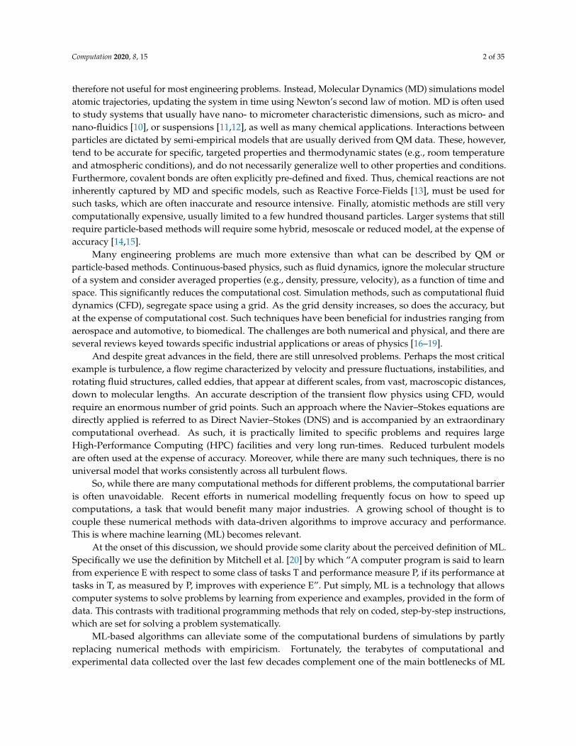
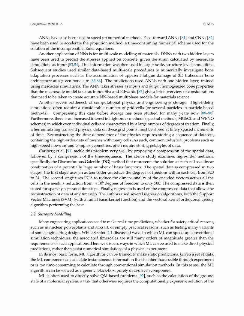
Traditionally, ML is often associated with signal and image processing, with topics like self-drivingvehicles, natural language processing, and optical character recognition coming to mind. Most industrialsectors are currently investing a significant amount of time and money into incorporating ML techniquesinto their practices for the betterment of their products and services. This increasing demand is alsoreflected in the massive rise of ML-related publications over the last few decades (Figure 1)

2000

2001

2002

2003

2004

2005

2006

2007

2008

2009

2010

2011

2012

2013

2014

2015

2016

2017

2018

Year

0

5000

10000

15000

20000

25000

Number of Publications

Figure 1. Number of ML-related publications as since 2000. Data obtained from Web of Science (https://apps.webofknowledge.com/)

Still, we believe that the recent success of ML is a glimpse of a technology that is yet to be fully used.We envision that ML will help shed light upon complex, multi-scale, multi-physics, engineering problemsand play a leading role in the continuation of today’s technological advancements. In this paper, we reviewsome of the work that has applied ML algorithms for the advancement of applied sciences and engineering.

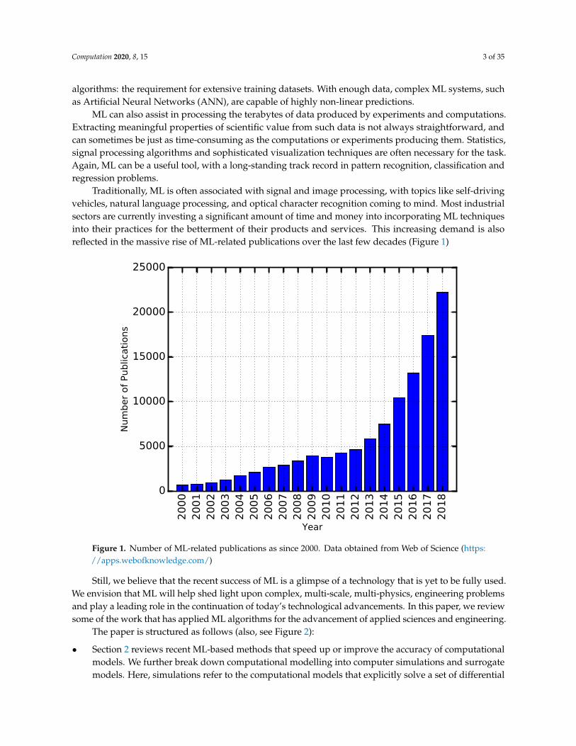
The paper is structured as follows (also, see Figure 2):

• Section 2 reviews recent ML-based methods that speed up or improve the accuracy of computationalmodels. We further break down computational modelling into computer simulations and surrogatemodels. Here, simulations refer to the computational models that explicitly solve a set of differential

https://apps.webofknowledge.com/

https://apps.webofknowledge.com/


equations that govern some physical processes. Instead, surrogate models refer to (semi-) empiricalmodels that replace and substantially simplify the governing equations, thus providing predictivecapabilities at a fraction of the time.

• Section 3 reviews ML-based methods that have been used in science and engineering to process largeand complex datasets and extract meaningful quantities.

• Section 4 reviews the use of ML for in virtual reality (VR). Although the research included in thissection could be a part of Sections 2 and 3, we do consider VR as a rather broad and unique branch ofscience. As such we believe that an independent section is more appropriate.

• Section 5 summarizes the current efforts for ML in engineering and discusses future perspectiveendeavors.

Please note that ML is a broad and complex topic. The purpose of this study is not to detail themathematical framework and specifics of every ML algorithm–a task better suited for a textbook–but tohighlight some important and relevant areas and direct an interested reader for further investigation.

Furthermore, the number of relevant disciplines to ML is too large to address in a single articleadequately. Our choice of scientific applications was not necessarily based on importance but wasnaturally driven by our research which is primarily in micro and nano flows, turbulence, multiphase flows,as well as in virtual environments.

2. Machine Learning for Computational Modelling

In this section, we review research that uses ML algorithms in scientific computing to achieve abetter balance between computational cost an accuracy. We divide the section into two subcategories:simulations and surrogate modelling. The first regards the application of ML to improve or speed upsimulation techniques (e.g., DFT, MD, and CFD), while the second refers to the use of ML to createreduced-order models that completely circumvent the need for the computationally expensive yet morephysically accurate simulations.

Figure 2. Overview of ML in science and engineering.


2.1. Simulations

An important goal in computational modelling and simulations is to find a good balance betweencomputational resources and accuracy. For example, in the absence of computational limits, QM-basedsimulations could be used to resolve complex, turbulent flows accurately; yet practically this is aninconceivable task. In this section, we present research that uses ML, aiming to improve the balancebetween accuracy and speed.

A good starting point is MD, a simulation technique that resolves the system down to the atomic scale.MD is based on Newtonian physics. Each atom is represented as a single point. Its electronic structure,the dynamics of which are described by QM, is ignored. The forces acting on the particles are calculated asthe gradient (i.e., spatial derivative) of the potentials: semi-empirical functions of the atomic coordinatesthat are usually derived through regressions from QM-based data. Once the forces are calculated, thesystem can evolve in time by integrating Newton’s second law of motion. The computational complexityof MD scales with the number of atoms and is usually limited to systems comprising a few hundredthousand particles.

The semi-empirical potentials used in MD, however, are not always accurate. Depending on thedata used for the extraction of these potentials, they might be tailored to specific situations, such as aspecific range of thermodynamic states (e.g., specific temperature and pressure). For example, there aremany potential functions available for the interaction of water molecules, each with its own strengths andweaknesses [21].

On the other hand, QM-based models resolve the system down to individual electrons, and assuch can accurately calculate the inter- and intra-molecular forces and interactions. Such techniques,however, are even more computationally demanding than MD, as atoms consist of many electrons thatare correlated with each other (i.e., quantum entanglement). Simulation methods such as DFT attempt tosimplify such many-body systems while still providing a quantum mechanical resolution. Regardless ofthe relative efficiency of DFT, however, it is still exceptionally computationally expensive compared tolarger-scale approaches.

To approximate the accuracy of QM-based methods, while retaining the computational advantage ofMD, ML-based methods, trained on QM data, can be used to derive accurate force-fields that can thenbe used by MD simulations. ML algorithms, such as ANNs [22–25], or Gaussian processes (GP) [26,27],have been trained, using DFT simulations, to reconstruct more general and accurate Potential EnergySurfaces (PES). The gradient of these PES provides the interatomic forces used by MD simulations.Chmiela et al. [27] have used Kernel Ridge Regression (KRR) to calculate interatomic forces by taking asinput the atomic coordinates. More recently, an ANN was trained to produce potentials that match theaccuracy of the computationally demanding but accurate Coupled-Cluster approach, a numerical schemethat can provide exact solutions to the time-independent Schröedinger equation, exceeding the accuracyof DFT [28].

Yet these potentials usually have a constant functional form. As such, they do not always generalizewell, and cannot accurately capture complex transitions such as chemical reactions and phase change.Hybrid models referred to as First Principle Molecular Dynamics (FPMD), use Newton’s laws to integratethe system in time (i.e., as in normal, classical MD), but use quantum mechanical simulations such as DFTto calculate the force-fields at each timestep. Variations of this approach attempt to limit the quantummechanical calculations only to when and where necessary [29]. ML algorithms, such as GP [30] orKRR [31], can reduce the computational cost of such approaches. The general idea is that when a new stateis encountered, the QM simulation will calculate the force-fields. The data, however, will also be usedto train some ML algorithm, such that, if any similar states are encountered, the fast ML component will


replace the computationally expensive QM simulation. Only when a new process is encountered are thecomputationally expensive QM simulations considered.

Such ML-based MD methods have successfully been used to simulate complex physical systems.ANNs have been used to simulate phase-change materials [32–35], make accurate predictions on the manyphases of silicon [36] and describe the structural properties of amorphous silicon [37], as well as efficientlyand accurately calculate infrared spectra of materials [38].

Clustering methods have also been used to evaluate the accuracy of classical MD force-fieldsfor various tasks. Pérez et al. [39] used a combination of Principal Component Analysis (PCA) andK-means classification to evaluate and categorize different force-fields used for modelling carbohydratesin MD. The PCA reduced the dimensionality of the system from individual positions and energeticsinto a two-dimensional orthonormal basis. The above reduction resulted in a high-level map indicatingsimilarities or differences between different force-fields. A hierarchical k-means clustering algorithm wasused on the PCA data to formally categorize the force-fields. Raval et al. [40] used k-means clustering ondata produced by MD simulations in order to assess the effectiveness of various classical force-fields insimulating the formation of specific proteins, i.e., for homology modelling, and propose alternatives thatcan mitigate the identified weaknesses.

For macroscopic fluid dynamics, on the other hand, the most common simulation technique is CFD.This method solves the fluid dynamics equations: the continuity equation, derived from the conservationof mass; the momentum equations, derived from the conservation of momentum; and the energy equation,derived from the conservation of energy. These equations ignore the molecular nature of fluids, and insteadconsider material properties as continuum functions of space and time. For a computer to solve theseequations, they must first be discretized. This is achieved by mapping the physical domain into a grid,and the equations are solved, using numerical methods, on discrete points (e.g., grid points, cell centers).As you increase the density of grid points the accuracy of the solution will also increase, at the expense ofcomputational resources.

In between the nanoscale (commonly treated with QM-based methods and MD) and macroscopicsystems (usually treated with CFD or a similar continuous method), there are physical problems thatlie in an intermediate scale. For example, microfluidic systems, systems with micrometer characteristicdimensions, are usually composed of a massive number of molecules (i.e., in liquid water there are∼1010 molecules in a cubic micrometer). Classical MD is, practically speaking, not an option. On theother hand, such scales are often too small for continuum methods. Models such as CFD are oftenincapable of capturing the complex physics that emerge at solid-liquid interfaces, such as variations in thethermodynamic properties [41,42], or accounting for surface roughness [43–45].

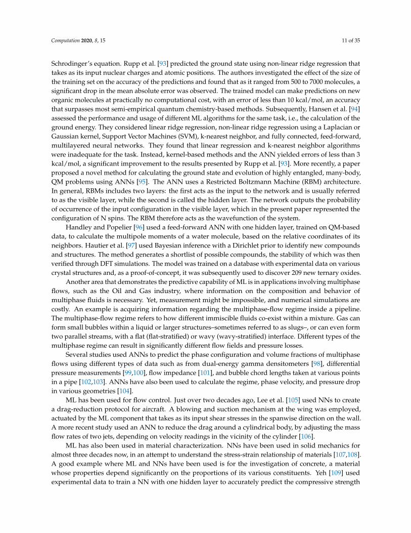
Instead, hybrid models have been proposed, in which the computationally favorable continuumsolver is predominantly used, while using a molecular solver for the under-resolved flow features.However, the MD simulations must run relatively frequently, sometimes at each macroscopic timestep,which significantly increases the computational requirements. Instead ANNs have been used to providemolecular-level information to a CFD solver, thus enabling a computationally efficient resolution of suchscales [46,47]. As with the QM-based simulations described above, the MD solver is only used whenit encounters relatively new states, i.e., states that are outside a pre-defined confidence interval frompreviously encountered states. As the simulation progresses and more states are encountered, the ANN isprimarily used. The ANN-based hybrid model captures the flow physics very well. Furthermore, while thethermal noise, inherent in MD simulations, prevented the continuum solver from converging satisfactory,the NN-based hybrid model suppressed the thermal fluctuations resulting in lower residuals and betterconvergence of the solution (Figure 3).


0 50 100 150 200Time Step

10-8

10-7

10-6

10-5

10-4

10-3

10-2

10-1

Velocity Residual

HybridNN with δu=0

NN with δu=5× 10−3

Figure 3. Comparison of the velocity residuals of a Couette flow through a microchannel as a function ofthe simulation timesteps. The blue curve corresponds to a hybrid, molecular-continuum solver, where themolecular solver is used at each timestep (blue). The green curve corresponds to a hybrid solver, where aNN replaces the molecular solver, but learns and adjusts its weights from the MD solver at each timestep(i.e., a vanishing confidence interval δu = 0). The orange curve corresponds to the same NN-based hybridsolver, but with the weights of the NN being adjusted only when the input data, in this case the velocity u,is outside of a confidence interval δu = 0 with respect to previously encountered velocities. Increasing theconfidence interval for re-training the NN decreases the residual which results in better convergence of thecontinuum solution. The figure is reconstructed from [47]

A long-standing, unresolved problem of fluid dynamics, is turbulence, a flow regime characterizedby unpredictable, time-dependent velocity and pressure fluctuations [48–51]. As mentioned in theintroduction, accurate resolution of all the turbulent scales requires an extremely fine grid, resultingin often prohibitive run-times. Instead, reduced turbulent models are often used at the expense of accuracy.A simplified approach is the Reynolds Averaged Navier–Stokes (RANS) equations that describe thetime-averaged flow physics, and consider turbulent fluctuations as an additional stress term, the Reynoldsstress, which encapsulates the velocity perturbations. This new term requires additional models to close thesystem of equations. While several such models are available, e.g., k-epsilon, k-ω, Spallart–Allmaras (SA),none of them is universal, meaning that different models are appropriate under different circumstances.Choosing the correct model, as well as appropriate parameters for the models (e.g., turbulence kineticenergy, and dissipation rate), is crucial for an accurate representation of the average behavior of theflow. Furthermore, this choice (particularly the choice of parameters) is often empirical, requiring atrial-and-error process to validate the model against experimental data.

ML has been used for turbulent modelling for the last two decades. Examples include the use ofANNs to predict the instantaneous velocity vector field in turbulent wake flows [52], or for turbulentchannel flows [53,54]. The use of data-driven methods for fluid dynamics has increased significantly overthe last few years, providing new modelling tools for complex turbulent flows [55].

A significant amount of effort is currently put into using ML algorithms to improve the accuracyof RANS models. GPs have been used to quantify and reduce uncertainties in RANS models [56].


Tracey et al. [57] used an ANN that takes flow properties as its input and reconstructs the SA closureequations. The authors study how different components of ML algorithms, such as the choice of the costfunction and feature scaling affect its performance. Overall, these ML-based models performed well for arange of different cases such as a 2D flat plate and transonic flow around 3D wings. The conclusion wasthat ML can be a useful tool in turbulence modelling, particularly if the ANN is trained on high-fidelitydata such as data from DNS or Large Eddy Simulation (LES) simulations. Similarly, Zhu et al. [58] trainedan ANN with one hidden layer on flow data using the SA turbulence model to predict the flow aroundan airfoil.

Deep Neural Networks (DNNs) incorporating up to 12 hidden layers have also been used to makeaccurate predictions of the Reynolds stress anisotropy tensor [59,60]. The ML model preserved Galileaninvariance, meaning that the choice of inertial frame of reference does not affect the predictions of theDNN. The authors of the paper further discuss the effect of more layers and nodes, indicating that more isnot necessarily better. They also stressed the importance of cross-validation in providing credence to theML model. Bayesian inference has been used to optimize the coefficients of RANS models [61,62], as wellas to derive functions that quantify and reduce the gap between the model predictions and high-fidelitydata, such as DNS data [63–65]. Similarly, a Bayesian Neural Network (BNN) has been used to improve thepredictions of RANS models and to specify the uncertainty associated with the prediction [66]. Randomforests have also been trained on high-fidelity data to quantify the error of RANS models based on meanflow features [67,68].

Another popular approach to turbulence is called Large Eddy Simulation (LES). LES resolves eddiesof a particular length scale. Unresolved scales, i.e., those that are comparable or smaller than the cellsize, are predicted through subgrid models. Several papers have successfully used ANN to replace thesesubgrid models [69,70]. Convolutional Neural Networks (CNNs) have also been used for the calculation ofsubgrid closure terms [71]. The model requires no a priori information, generalizes well to various types offlow, and produces results that compare well with current LES closure models. Similarly, Maulik et al. [72]used a DNN, taking as input vorticity and stream function stencils that predicts a dynamic, time andspace-dependent closure term for the subgrid models.

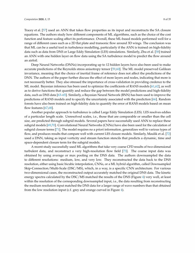
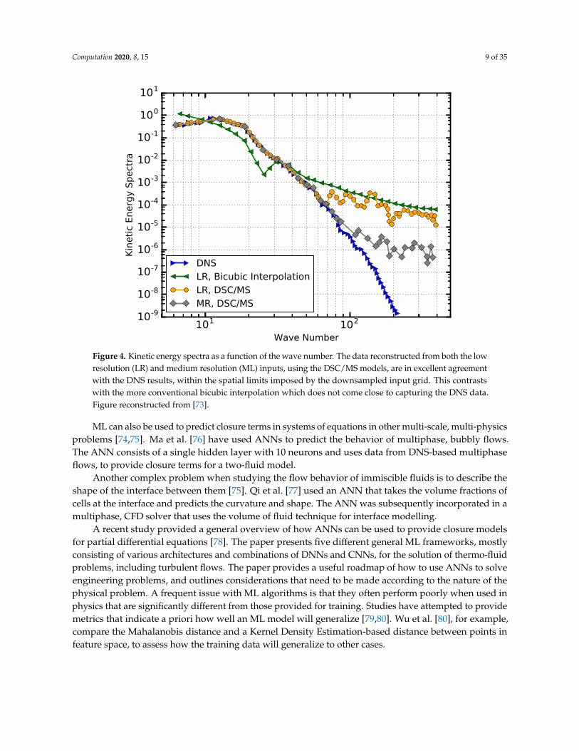
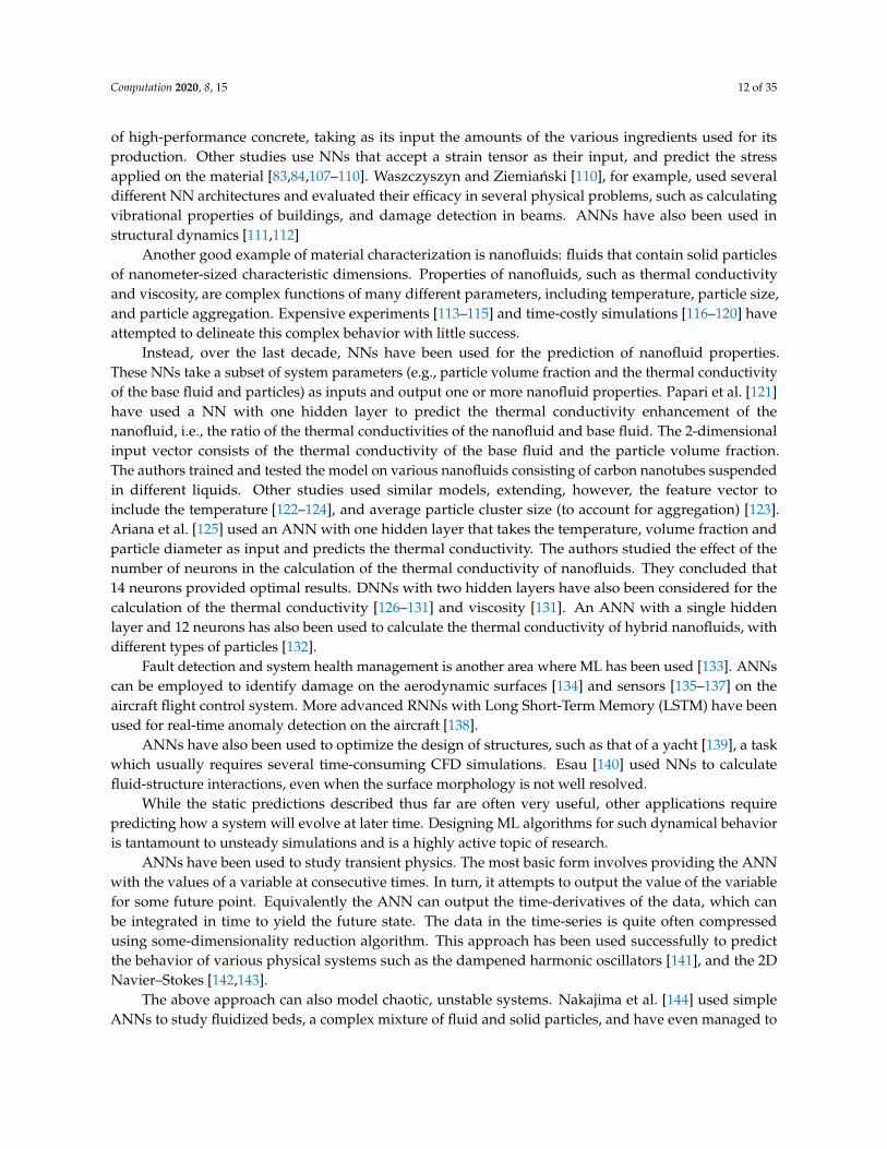
A recent study successfully used ML algorithms that take very coarse CFD results of two-dimensionalturbulent data, and reconstruct a very high-resolution flow field [73]. The coarse input data wasobtained by using average or max pooling on the DNS data. The authors downsampled the datato different resolutions: medium, low, and very low. They reconstructed the data back to the DNSresolution, either using basic bicubic interpolation, CNNs, or a ML hybrid algorithm, called DownsampledSkip-Connection/Multi-Scale (DSC/MS), which, in a way, is a specific CNN architecture. For varioustwo-dimensional cases, the reconstructed output accurately matched the original DNS data. The kineticenergy spectra calculated by the DSC/MS matched the results of the DNS (Figure 4) very well, at leastwithin the resolution of the corresponding downsampled input, i.e., the data resulting from reconstructingthe medium resolution input matched the DNS data for a larger range of wave numbers than that obtainedfrom the low resolution input (c.f. grey and orange curved in Figure 4).


101 102

Wave Number

10-9

10-8

10-7

10-6

10-5

10-4

10-3

10-2

10-1

100

101

Kin

eti

c E

ne

rgy

Sp

ect

ra

DNSLR, Bicubic InterpolationLR, DSC/MSMR, DSC/MS

Figure 4. Kinetic energy spectra as a function of the wave number. The data reconstructed from both the lowresolution (LR) and medium resolution (ML) inputs, using the DSC/MS models, are in excellent agreementwith the DNS results, within the spatial limits imposed by the downsampled input grid. This contrastswith the more conventional bicubic interpolation which does not come close to capturing the DNS data.Figure reconstructed from [73].

ML can also be used to predict closure terms in systems of equations in other multi-scale, multi-physicsproblems [74,75]. Ma et al. [76] have used ANNs to predict the behavior of multiphase, bubbly flows.The ANN consists of a single hidden layer with 10 neurons and uses data from DNS-based multiphaseflows, to provide closure terms for a two-fluid model.

Another complex problem when studying the flow behavior of immiscible fluids is to describe theshape of the interface between them [75]. Qi et al. [77] used an ANN that takes the volume fractions ofcells at the interface and predicts the curvature and shape. The ANN was subsequently incorporated in amultiphase, CFD solver that uses the volume of fluid technique for interface modelling.

A recent study provided a general overview of how ANNs can be used to provide closure modelsfor partial differential equations [78]. The paper presents five different general ML frameworks, mostlyconsisting of various architectures and combinations of DNNs and CNNs, for the solution of thermo-fluidproblems, including turbulent flows. The paper provides a useful roadmap of how to use ANNs to solveengineering problems, and outlines considerations that need to be made according to the nature of thephysical problem. A frequent issue with ML algorithms is that they often perform poorly when used inphysics that are significantly different from those provided for training. Studies have attempted to providemetrics that indicate a priori how well an ML model will generalize [79,80]. Wu et al. [80], for example,compare the Mahalanobis distance and a Kernel Density Estimation-based distance between points infeature space, to assess how the training data will generalize to other cases.


ANNs have also been used to speed up numerical methods. Feed-forward ANNs [81] and CNNs [82]have been used to accelerate the projection method, a time-consuming numerical scheme used for thesolution of the incompressible, Euler equations.

Another application of NNs is for multi-scale modelling of materials. DNNs with two hidden layershave been used to predict the stresses applied on concrete, given the strain calculated by mesoscalesimulations as input [83,84]. This information was then used in larger-scale, structure-level simulations.Subsequent studies used similar data-based multi-scale procedures to numerically investigate boneadaptation processes such as the accumulation of apparent fatigue damage of 3D trabecular bonearchitecture at a given bone site [85,86]. The predictions used ANNs with one hidden layer, trainedusing mesoscale simulations. The ANN takes stresses as inputs and output homogenized bone propertiesthat the macroscale model takes as input. Sha and Edwards [87] give a brief overview of considerationsthat need to be taken to create accurate NN-based multiphase models for materials science.

Another severe bottleneck of computational physics and engineering is storage. High-fidelitysimulations often require a considerable number of grid cells (or several particles in particle-basedmethods). Compressing this data before storage has been studied for many years now [88–90].Furthermore, there is an increased interest in high-order methods (spectral methods, MUSCL and WENOschemes) in which even individual cells are characterized by a large number of degrees of freedom. Finally,when simulating transient physics, data on these grid points must be stored at finely spaced incrementsof time. Reconstructing the time-dependence of the physics requires storing a sequence of datasets,containing the high-order data of meshes with many cells. As such, common industrial problems such ashigh-speed flows around complex geometries, often require storing petabytes of data.

Carlberg et al. [91] tackle this problem very well by proposing a compression of the spatial data,followed by a compression of the time-sequence. The above study examines high-order methods,specifically the Discontinuous Galerkin (DG) method that represents the solution at each cell as a linearcombination of a potentially large number of basis functions. The spatial data is compressed in twostages: the first stage uses an autoencoder to reduce the degrees of freedom within each cell from 320to 24. The second stage uses PCA to reduce the dimensionality of the encoded vectors across all thecells in the mesh, a reduction from ∼ 106 degrees of freedom to only 500. The compressed data is thenstored for sparsely separated timesteps. Finally, regression is used on the compressed data that allows thereconstruction of data at any timestep. The authors used several regression algorithms, with the SupportVector Machines (SVM) (with a radial basis kernel function) and the vectoral kernel orthogonal greedyalgorithm performing the best.

2.2. Surrogate Modelling

Many engineering applications need to make real-time predictions, whether for safety-critical reasons,such as in nuclear powerplants and aircraft, or simply practical reasons, such as testing many variantsof some engineering design. While Section 2.1 discussed ways in which ML can speed up conventionalsimulation techniques, the associated timescales are still many orders of magnitude greater than therequirements of such applications. Here we discuss ways in which ML can be used to make direct physicalpredictions, rather than assist numerical simulations of a physical experiment.

In its most basic form, ML algorithms can be trained to make static predictions. Given a set of data,the ML component can calculate instantaneous information that is either inaccessible through experimentor is too time-consuming to calculate through conventional simulation methods. In this sense, the MLalgorithm can be viewed as a generic, black-box, purely data-driven component.

ML is often used to directly solve QM-based problems [92], such as the calculation of the groundstate of a molecular system, a task that otherwise requires the computationally expensive solution of the


Schrodinger’s equation. Rupp et al. [93] predicted the ground state using non-linear ridge regression thattakes as its input nuclear charges and atomic positions. The authors investigated the effect of the size ofthe training set on the accuracy of the predictions and found that as it ranged from 500 to 7000 molecules, asignificant drop in the mean absolute error was observed. The trained model can make predictions on neworganic molecules at practically no computational cost, with an error of less than 10 kcal/mol, an accuracythat surpasses most semi-empirical quantum chemistry-based methods. Subsequently, Hansen et al. [94]assessed the performance and usage of different ML algorithms for the same task, i.e., the calculation of theground energy. They considered linear ridge regression, non-linear ridge regression using a Laplacian orGaussian kernel, Support Vector Machines (SVM), k-nearest neighbor, and fully connected, feed-forward,multilayered neural networks. They found that linear regression and k-nearest neighbor algorithmswere inadequate for the task. Instead, kernel-based methods and the ANN yielded errors of less than 3kcal/mol, a significant improvement to the results presented by Rupp et al. [93]. More recently, a paperproposed a novel method for calculating the ground state and evolution of highly entangled, many-body,QM problems using ANNs [95]. The ANN uses a Restricted Boltzmann Machine (RBM) architecture.In general, RBMs includes two layers: the first acts as the input to the network and is usually referredto as the visible layer, while the second is called the hidden layer. The network outputs the probabilityof occurrence of the input configuration in the visible layer, which in the present paper represented theconfiguration of N spins. The RBM therefore acts as the wavefunction of the system.

Handley and Popelier [96] used a feed-forward ANN with one hidden layer, trained on QM-baseddata, to calculate the multipole moments of a water molecule, based on the relative coordinates of itsneighbors. Hautier et al. [97] used Bayesian inference with a Dirichlet prior to identify new compoundsand structures. The method generates a shortlist of possible compounds, the stability of which was thenverified through DFT simulations. The model was trained on a database with experimental data on variouscrystal structures and, as a proof-of-concept, it was subsequently used to discover 209 new ternary oxides.

Another area that demonstrates the predictive capability of ML is in applications involving multiphaseflows, such as the Oil and Gas industry, where information on the composition and behavior ofmultiphase fluids is necessary. Yet, measurement might be impossible, and numerical simulations arecostly. An example is acquiring information regarding the multiphase-flow regime inside a pipeline.The multiphase-flow regime refers to how different immiscible fluids co-exist within a mixture. Gas canform small bubbles within a liquid or larger structures–sometimes referred to as slugs–, or can even formtwo parallel streams, with a flat (flat-stratified) or wavy (wavy-stratified) interface. Different types of themultiphase regime can result in significantly different flow fields and pressure losses.

Several studies used ANNs to predict the phase configuration and volume fractions of multiphaseflows using different types of data such as from dual-energy gamma densitometers [98], differentialpressure measurements [99,100], flow impedance [101], and bubble chord lengths taken at various pointsin a pipe [102,103]. ANNs have also been used to calculate the regime, phase velocity, and pressure dropin various geometries [104].

ML has been used for flow control. Just over two decades ago, Lee et al. [105] used NNs to createa drag-reduction protocol for aircraft. A blowing and suction mechanism at the wing was employed,actuated by the ML component that takes as its input shear stresses in the spanwise direction on the wall.A more recent study used an ANN to reduce the drag around a cylindrical body, by adjusting the massflow rates of two jets, depending on velocity readings in the vicinity of the cylinder [106].

ML has also been used in material characterization. NNs have been used in solid mechanics foralmost three decades now, in an attempt to understand the stress-strain relationship of materials [107,108].A good example where ML and NNs have been used is for the investigation of concrete, a materialwhose properties depend significantly on the proportions of its various constituents. Yeh [109] usedexperimental data to train a NN with one hidden layer to accurately predict the compressive strength


of high-performance concrete, taking as its input the amounts of the various ingredients used for itsproduction. Other studies use NNs that accept a strain tensor as their input, and predict the stressapplied on the material [83,84,107–110]. Waszczyszyn and Ziemianski [110], for example, used severaldifferent NN architectures and evaluated their efficacy in several physical problems, such as calculatingvibrational properties of buildings, and damage detection in beams. ANNs have also been used instructural dynamics [111,112]

Another good example of material characterization is nanofluids: fluids that contain solid particlesof nanometer-sized characteristic dimensions. Properties of nanofluids, such as thermal conductivityand viscosity, are complex functions of many different parameters, including temperature, particle size,and particle aggregation. Expensive experiments [113–115] and time-costly simulations [116–120] haveattempted to delineate this complex behavior with little success.

Instead, over the last decade, NNs have been used for the prediction of nanofluid properties.These NNs take a subset of system parameters (e.g., particle volume fraction and the thermal conductivityof the base fluid and particles) as inputs and output one or more nanofluid properties. Papari et al. [121]have used a NN with one hidden layer to predict the thermal conductivity enhancement of thenanofluid, i.e., the ratio of the thermal conductivities of the nanofluid and base fluid. The 2-dimensionalinput vector consists of the thermal conductivity of the base fluid and the particle volume fraction.The authors trained and tested the model on various nanofluids consisting of carbon nanotubes suspendedin different liquids. Other studies used similar models, extending, however, the feature vector toinclude the temperature [122–124], and average particle cluster size (to account for aggregation) [123].Ariana et al. [125] used an ANN with one hidden layer that takes the temperature, volume fraction andparticle diameter as input and predicts the thermal conductivity. The authors studied the effect of thenumber of neurons in the calculation of the thermal conductivity of nanofluids. They concluded that14 neurons provided optimal results. DNNs with two hidden layers have also been considered for thecalculation of the thermal conductivity [126–131] and viscosity [131]. An ANN with a single hiddenlayer and 12 neurons has also been used to calculate the thermal conductivity of hybrid nanofluids, withdifferent types of particles [132].

Fault detection and system health management is another area where ML has been used [133]. ANNscan be employed to identify damage on the aerodynamic surfaces [134] and sensors [135–137] on theaircraft flight control system. More advanced RNNs with Long Short-Term Memory (LSTM) have beenused for real-time anomaly detection on the aircraft [138].

ANNs have also been used to optimize the design of structures, such as that of a yacht [139], a taskwhich usually requires several time-consuming CFD simulations. Esau [140] used NNs to calculatefluid-structure interactions, even when the surface morphology is not well resolved.

While the static predictions described thus far are often very useful, other applications requirepredicting how a system will evolve at later time. Designing ML algorithms for such dynamical behavioris tantamount to unsteady simulations and is a highly active topic of research.

ANNs have been used to study transient physics. The most basic form involves providing the ANNwith the values of a variable at consecutive times. In turn, it attempts to output the value of the variablefor some future point. Equivalently the ANN can output the time-derivatives of the data, which canbe integrated in time to yield the future state. The data in the time-series is quite often compressedusing some-dimensionality reduction algorithm. This approach has been used successfully to predictthe behavior of various physical systems such as the dampened harmonic oscillators [141], and the 2DNavier–Stokes [142,143].

The above approach can also model chaotic, unstable systems. Nakajima et al. [144] used simpleANNs to study fluidized beds, a complex mixture of fluid and solid particles, and have even managed to


identify bifurcating patterns [145], indicative of instabilities. The predictive capability of these methods,however, is usually limited to only a short time interval past that of the training set.

For predictions over a longer period of time, ANNs can re-direct their output and append it to thetime-series corresponding to its input, and use it for the calculation of data at successively longer periods.However, chaotic systems are susceptible to initial and boundary conditions. Therefore, an accuratelong-term prediction requires careful selection and pre-processing of the features [146]; otherwise, the errorfor highly chaotic systems increases with continuously longer times [147,148]. More recently, regressionforests [149], as well LSTM [150] have been used for transient flow physics.

A recent breakthrough in dynamic prediction is called Sparse Identification of Non-linear Dynamics(SINDy) [151]. SINDy reconstructs governing equations, based on data measured across different times.In general, the user empirically selects several possible non-linear functions for the input features. Usingsparse regression, SINDy then selects the functions that are relevant to the input data, thus recreating anattractor corresponding to the physical problem. The reconstructed equations can then be used without theneed for ML, and can theoretically make predictions outside the scope represented by the training data.

Lui and Wolf [152] used a methodology similar to SINDy, the main difference being that DNNs wereused to identify the non-linear functions describing the problem, rather than manually and empiricallyselecting them. The authors tested their method successfully on non-linear oscillators, as well ascompressible flows around a cylinder.

SINDy sounds like the optimal solution to dynamic prediction, as it extracts a relatively globalfunction that is not necessarily restricted to the confines of the training data. Pan and Duraisamy [153],however, identified that while SINDy is near perfect for systems described by polynomial functions,its performance drops significantly when considering nonpolynomial systems. The authors showcasedthis for the case of a nonrational, nonpolynomial oscillator. They attributed the behavior to the complexityof the dynamic behavior of the system that cannot be decomposed into a sparse number of functions.The paper concluded that for such general cases, the fundamental ANN-based way of dynamic modellingis more appropriate.

Efforts are also directed into incorporating our theoretical knowledge of physics into the MLalgorithms, rather than using them as trained, black-box tools. Bayesian inference has long been linkedto numerical analysis (i.e., Bayesian numerical analysis), and has recently been used for numericalhomogenization [154], i.e., finding solutions to partial differential equations. Subsequent studies have usedGP regression that, given the solution of a physical problem, it can discover the underlying linear [155,156]and non-linear [157] differential equations, such as the Navier–Stokes and Schröedinger equations.Alternatively, similar GP-based methods can infer solutions, given the governing differential equationsas well as (potentially noisy) initial conditions [158]. A particularly attractive feature of GPs is that theyenable accurate predictions with a small amount of data.

While GPs generally allow the injection of knowledge through the covariance operators, creatingphysics-informed ANNs feels like a more challenging task considering the inherent black-box-natureof traditional ANNs. ANNs can be used for automatic differentiation [159], enabling the calculation ofderivatives of a broad range of functions.

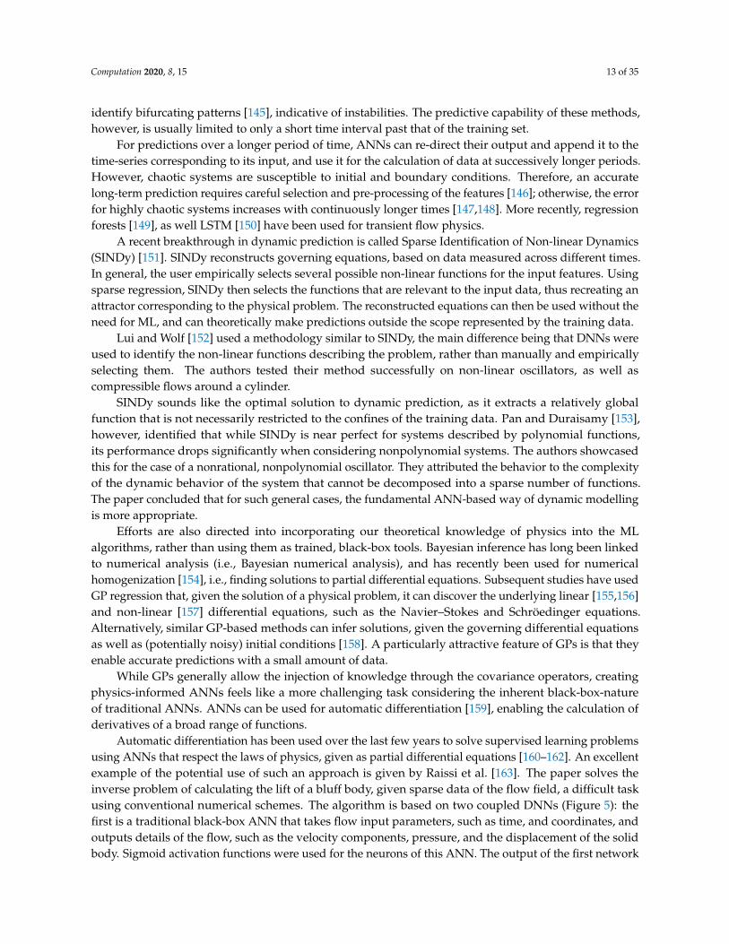
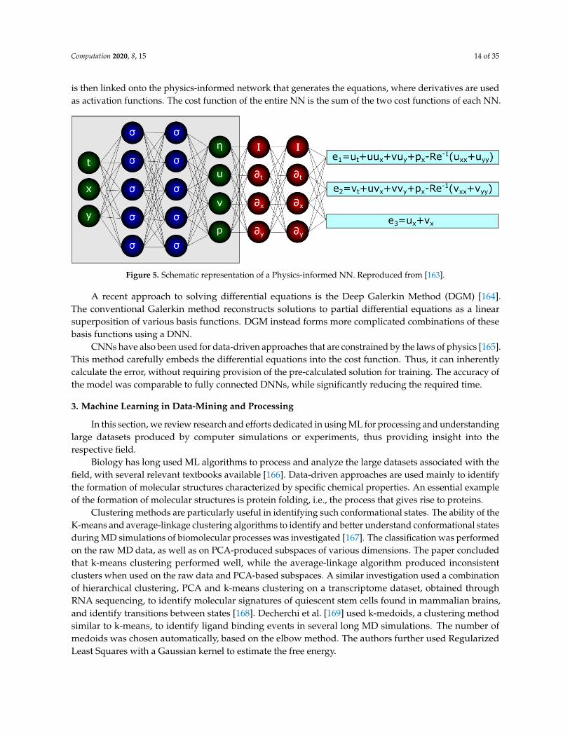
Automatic differentiation has been used over the last few years to solve supervised learning problemsusing ANNs that respect the laws of physics, given as partial differential equations [160–162]. An excellentexample of the potential use of such an approach is given by Raissi et al. [163]. The paper solves theinverse problem of calculating the lift of a bluff body, given sparse data of the flow field, a difficult taskusing conventional numerical schemes. The algorithm is based on two coupled DNNs (Figure 5): thefirst is a traditional black-box ANN that takes flow input parameters, such as time, and coordinates, andoutputs details of the flow, such as the velocity components, pressure, and the displacement of the solidbody. Sigmoid activation functions were used for the neurons of this ANN. The output of the first network


is then linked onto the physics-informed network that generates the equations, where derivatives are usedas activation functions. The cost function of the entire NN is the sum of the two cost functions of each NN.

Figure 5. Schematic representation of a Physics-informed NN. Reproduced from [163].

A recent approach to solving differential equations is the Deep Galerkin Method (DGM) [164].The conventional Galerkin method reconstructs solutions to partial differential equations as a linearsuperposition of various basis functions. DGM instead forms more complicated combinations of thesebasis functions using a DNN.

CNNs have also been used for data-driven approaches that are constrained by the laws of physics [165].This method carefully embeds the differential equations into the cost function. Thus, it can inherentlycalculate the error, without requiring provision of the pre-calculated solution for training. The accuracy ofthe model was comparable to fully connected DNNs, while significantly reducing the required time.

3. Machine Learning in Data-Mining and Processing

In this section, we review research and efforts dedicated in using ML for processing and understandinglarge datasets produced by computer simulations or experiments, thus providing insight into therespective field.

Biology has long used ML algorithms to process and analyze the large datasets associated with thefield, with several relevant textbooks available [166]. Data-driven approaches are used mainly to identifythe formation of molecular structures characterized by specific chemical properties. An essential exampleof the formation of molecular structures is protein folding, i.e., the process that gives rise to proteins.

Clustering methods are particularly useful in identifying such conformational states. The ability of theK-means and average-linkage clustering algorithms to identify and better understand conformational statesduring MD simulations of biomolecular processes was investigated [167]. The classification was performedon the raw MD data, as well as on PCA-produced subspaces of various dimensions. The paper concludedthat k-means clustering performed well, while the average-linkage algorithm produced inconsistentclusters when used on the raw data and PCA-based subspaces. A similar investigation used a combinationof hierarchical clustering, PCA and k-means clustering on a transcriptome dataset, obtained throughRNA sequencing, to identify molecular signatures of quiescent stem cells found in mammalian brains,and identify transitions between states [168]. Decherchi et al. [169] used k-medoids, a clustering methodsimilar to k-means, to identify ligand binding events in several long MD simulations. The number ofmedoids was chosen automatically, based on the elbow method. The authors further used RegularizedLeast Squares with a Gaussian kernel to estimate the free energy.


Most clustering methods discussed above are referred to as structure-based methods, where thetime-dependent data produced from MD simulations (or experiments) is treated as one large data set, or asa sequence of independent data through which the clustering is refined. Other studies have used clusteringmethods more conducive to dynamic data [170]. Such methods are referred to as dynamic-based clusteringmethods, and consider the simulation data in a more natural, time-dependent manner (e.g., by consideringthe timesteps as steps along a Markov chain). Dynamic-based clustering attempts to partition the dynamicdata into meta-stable states: states that persist for long periods. While the results from structure-and dynamics-based methods are often similar, they also frequently result in major differences [171].Noé et al. [172] used the Perron Cluster Cluster Analysis (PCCA) method to study the effect of metastabilityon the folding dynamics of proteins. More robust variants of PCCA have also been derived [173] whichwere subsequently used for clustering gene expression data with application in breast cancer research [174].

While ANNs have been used in biology for many years [175], such techniques have become moreprominent over the last decade [176,177]. The above is particularly true for protein-DNA binding, a processwhich biophysical models seem to fall short [178] currently. Fully connected ANNs with many inputs,corresponding to genetic features, have been used to predict RNA splicing, thus evaluating the effect ofdifferent genetic variants [179]. CNNs have also been used to predict protein-binding, outperformingprevious equivalent models [180]. Zeng et al. [181] investigated the effect of various CNN architectures ontheir predictive capability on DNA–protein binding. While the paper goes into detail regarding variouspossible CNN considerations, the overall conclusion is that a larger number of filters will result in learningmore productive sequence features. Other CNN-based architectures have been used in genetics, such as inclassifying DNA sequences [182] and identify the function of noncoding genomic variations [183].

ML has also been used for Computer-Aided Detection (CAD), i.e., computer solutions that assistdiagnostic medicine. An important example of the application of ML for CAD is in lung cancer detection,one of the leading causes of death worldwide. While lung cancer can effectively be treated and evencured if detected early, it can often be left undiagnosed, even by experienced medical professionals,until it reaches more advanced stages. Given appropriate data, e.g., provided in the form of scannedimages, ML algorithms can help with cancer detection in two respects: (i) first, they can identify thediseased region, a process called segmentation; (ii) they can classify cancers (benign, aggressive etc.).Krishnaiah et al. [184] discuss the potential use of different classifiers for the early detection of lung cancer.The paper considered Naive Bayesian classifiers, association rules (if-then rules), decision trees, and NNs.Subsequent studies used feed-forward NNs to detect lung cancer from Computerized Tomography (CT)scans [185]. The authors initially applied segmentation in the form of thresholding and morphologicaloperations to identify the lungs. Statistical parameters were then calculated based on the pixel intensitiesof the segmented images. The parameters used were the mean, standard deviation, skewness, kurtosis,and fifth and sixth central moments. These compiled the feature vector used as input to the ANN, whichin turn classified the case as cancerous or not. D’Cruz et al. [186] have used a combination of NNs andgenetic algorithms to organize data, provided in the form of X-Rays, CT scans, MRIs etc. Following featureextraction on the raw data, a fully connected, feed-forward NN was used to classify the image into normalor abnormal. If an instance were classified as abnormal, the genetic algorithm would further classify it intocancerous and non-cancerous.

More complicated NNs, such as DNNs, CNNs and Autoencoders have also been used for CAD.Autoencoders have been used to extract features from lung nodules found on CT scans that can then beused to classify the nodules as malignant or benign [187]. Song et al. [188] compared the effectiveness ofDNNs, CNNs and Autoencoders in classifying lung nodules from CT scans into benign and malignant.The paper concluded that CNNs outperform the other two methods. A similar CNN architecture, e.g., threeconvolutional and two pooling layers, has also been used to classify lung tumors into adenocarcinoma,squamous cell carcinoma, and small cell carcinoma [189]. Another study [190] defined a protocol that takes


as its input a CT scan, segments it using thresholding to identify the lung region, and classifies the detectednodules. The authors claim that directly using a CNN on the thresholded data is insufficient and resultsin many false positives. Instead, they first used a U-net architecture, a specific CNN architecture thatcan increase the resolution of the input data through upsampling layers rather than reducing it throughpooling layers. The U-net identified potential nodules in the lungs that were then classified into cancerousor non-cancerous by a conventional 3D CNN architecture. Subsequent studies considered several CADpipelines that include CNN architectures, achieving quite a high level of accuracy [191–193]. A recentdeep learning algorithm for lung cancer detection combined CNNs into an autoencoder [194]. A 3D CNN,acting as the encoder, reduces a CT scan into a representation, which is then decoded by another CNN.At the same time, the generated representation was also fed to a fully connected NN to be classified ascancerous or benign. Please note that a single cost function, including both the loss from the autoencoderas well as the classification loss, was used for training.

ML has similarly been used for other types of cancer, such as breast cancer [195–199] andprostate cancer [200–203]. It has also been used for other diseases such as Alzheimer’s [204–207] andParkinson’s [208–211] disease.

The increasing use of microfluidics in biomedical applications is also now being complemented withdata-driven approaches to analyze the produced data [212,213]. Berg et al. [214] designed a hand-helddevice attached to a smartphone that incorporates a 96-well plate for enzyme-linked immunosorbentassay, the gold standard for modern medical diagnostic tests. The camera of the phone reads the testresults, subsequently transmitting them to servers that generate diagnostic results through ML algorithms,specifically adaptive boosting (i.e., AdaBoost).

The anti-malware industry is now using ML to better shield computer systems from software threats(viruses, adware, spyware, etc.). One way of identifying and categorizing malicious software is to run it insome controlled environment (aka a sandbox) and analyze its behavior during runtime. In turn, clusteringcan be used to identify new classes of malware [215,216], while classification can be used to identify apiece of software as belonging to a specific malware class [217]. A combination of both clustering andclassification seems to provide even better results [218].

An alternative to dynamic analysis for malware detection is to take the object code (binary) of themalware executable, reshape it into a 2D array and present it as a greyscale image. The idea is that malwarewith similar features should also produce images with similar patterns, and can thus be classified usingimage processing methods such as K-Nearest Neighbors (KNN) [219]. Studies used PCA on the greyscaleimages, and classified the reduced data using ANNs, KNNs and SVMs, with KNNs outperforming theother methods [220]

Another field in which ML has been used significantly is astronomy [221–223], where advancedtelescopes provide an abundance of imaging data that needs to be processed [224,225]. While ML methodssuch as ANN have been used for almost 30 years [226], more recent works focus on CNNs, due to theirability to process and analyze images in a relatively computationally efficient way. CNNs have been usedto understand the morphology of galaxies [227–229], predict photometric redshifts [230,231], detect galaxyclusters [232], identify gravitational lenses [233–236] and reconstruction of images [237]

Video classification is yet another field that keeps improving along with advances in ML.Karpathy et al. [238] have used CNNs to classify sports-related videos found on YouTube into theircorresponding sports. They considered various architectures to effectively embed the time framesof the video into the CNN, as well as improving the computational cost required for training thenetwork. Subsequent studies suggested several different CNN- and RNN-based architectures for videoclassification [239–244]

Knowledge distillation refers to an approach wherein a complex ML algorithm, commonly called theteacher, is trained on a large set of data and is subsequently used to train simpler ML models, referred to


as the students, at a lower computational cost. Bhardwaj et al. [245] used knowledge distillation to classifyvideos efficiently. The teacher was trained using every time frame of each video. The student insteadconsidered only a small subset of time frames. The student’s cost function attempted to minimize themismatch between the results of the teacher and student. Different CNN and RNN architectures wereconsidered for the teacher and student.

Another active research topic involving ML is predicting a human’s future behavior. ML algorithms(mostly involving CNNs or RNNs) might consider human interactions [246–250], the context of a person(i.e., location and surroundings) [251–253], and characteristics of the person (e.g., facial expressions) [254],to predict the future path in which the person will follow. More recently, a study used LSTM and managedto predict not only the future path of the person but also her future activity [255].

4. Machine Learning and Virtual Environments

Data-driven features, automation and machine learning form a new framework for improving thedecision-making process in several disciplines (i.e., manufacturing, medicine, e-commerce and defenseamong others) [256–259]. To this end, ML is enabling data visualization and simulation of complex systemsin an immersive manner with the use of emerging technologies such as virtual reality (VR) and AugmentedReality (AR), as well as virtual and digital prototypes, environments, and models [260]. The immersiveand interactive visualization of data through VR and AR can increase productivity, reduce developmentcosts and provide a means of testing various systems in a computer-generated environment [258,259,261].

In the automotive engineering research sector, VR applications, such as VR driving simulators, requirethe realistic interaction between the user and agent vehicles (i.e., computer-controlled), also known asNon-Player Characters (NPCs) that recreate seamless traffic flow conditions and accident scenarios [262].A large number of VR driving simulators use ML algorithms to train the NPC vehicles and VRinfrastructure (i.e., road network and wireless communications) in order to interact and respond tovehicular or driver simulations and evaluations in a realistic manner [262–264].

Charissis and Papanastasiou [265] have developed a series of VR driving simulators which use ML totrain the agent vehicles for optimal operation of traffic flow, and for recreation of accident scenarios basedon real-life information provided by the relevant traffic monitoring and police authorities. The simulationscenarios recreated with the use of ML-trained agent vehicles were varying from a rear collision due tolow visibility weather conditions scenario [261,262] to the rear and side collisions due to driver distractionby in-vehicle infotainment systems [266,267]. The ML component further enriches the simulations touse Vehicular Ad-Hoc Networks systems (VANETs). These were simulated using an NS-3 networksimulator and were embedded in the VR driving environment to more realistically portray existing networkcommunication patterns and issues [265,266]. The driving simulator is further trained, improved andenhanced with additional scenarios and systems to produce realistic VR simulations, suitable for evaluatingcomplex Human-Machine Interfaces (HMI) that include gesture recognition and AR [261,267]. The useof ML for biomechanical gesture recognition in VR applications is explored also by Feng and Fei [268],who combined information fusion theory and ML to effectively train a gesture recognition system whichentailed ten different gestures. The proposed system aimed to resolve recognition and positioning issues,caused by traditional gesture segmentations.

The requirement for realistic responses from agents further sparked the development of an IntelligentTutoring System (ITS), which employed ML to train a VR driving simulator [263]. The ML training ofthe NPC agents is of major importance as it enables a more natural behavior, something that is essentialfor realistic interaction with the neighboring agent vehicles in various driving simulation scenarios [269].Lim et al. [270] discuss the rationale for the development of adaptive, affective and autonomous NPCs,where the agents strive towards the achievement of short term goals and adapting relative to user’s choices


and responses [270]. Notably, the affective and autonomous agents operating within a VR simulatedenvironment could significantly enhance the simulation immersion [262,263,271].

Yet the relation between VR and ML can also be inverted: the VR can produce realistic data used fortraining an ML component. Vazquez et al. [272] describe the development and use of virtual environmentsthat could automatically provide precise and rich annotations, in order to train pedestrian detectionsystems for vehicular applications. The rationale for using virtual environments for ML is the fact thata typical annotation process relies on learnt classifiers that require human attention which is both anintensive and a subjective task. For this reason, collecting training annotations could be replaced from thetypical avenues of camera and sensor-based to realistic virtual environments that replicate faithfully therequired visual information for the annotations.

Extending the synergy between VR and ML in multidisciplinary applications, Vazquez et al. [273]present a VR-based deep learning (DL) development environment which enables the users to deploy aDL model for image classification [274,275]. This system offers a VR immersive environment in whichthe user can manually select and train the system. Although the particular system is aiming to supportbiomedical professionals, the system could be adopted by other disciplines with the introduction of otherimage sequences required for different classification models [273].

Digital Twins is the use of VR to create digital replicas of engineering systems, equipment, orcomplete facilities, such as oil-rig installations, enabling the efficient monitoring, evaluation of suchsystems, as well as identifying potential sources of malfunction [276,277]. Recently, ML has been usedwith twin technologies. The virtual representation of identical real-life systems (i.e., oil-rig installations)and the incorporation of ML in such models for simulation and monitoring purposes is presented byMadni et al. [278]. In this study, the digital twin systems are categorized into 4 distinctive levels namelythe Pre-Digital Twin, Digital Twin, Adaptive Digital Twin and Intelligent Digital Twin, with the latterpresenting the most advanced form. The last two levels incorporate ML, yet only the Intelligent DigitalTwin incorporates both supervised ML (i.e., operator’s preferences) and unsupervised ML to distinguishvarious patterns and structures/items appearing in different operational situations. The digital twinmodelling and simulation approach is also explored by Jaensch et al. [279], where they present a digitaltwin platform that incorporates both model-based and data-driven methods. Their approach resolvestypical manufacturing and operational issues in a timely and cost-efficiently manner, in contrast tostandard methods.

A different way in which ML can improve VR is in networking. It is becoming increasinglyimportant that VR applications are operated over wireless networks. This presents fresh opportunities forcollaborative VR environments and immersive experiences access by remotely located users. Such activitiescould enable the monitoring and maintenance of systems remotely (i.e., digital twin systems), throughimmersive wireless VR environments. The transmission of VR data through wireless networks, however,could be hindered by poor network performance resulting in poor Quality-of-Service (QoS) [280]. Notably,this occurs in different types of networks due to the volume of data required for VR applications. In thiscase, Chen et al. [280], propose a novel solution based on ML framework of Echo State Networks (ESNs) inorder to mitigate and reduce this issue specifically for Small Cell Networks (SCNs). Further research aimingto minimize such issues by Chen et al. [281] present a data correlation-aware resource management forwireless VR applications. The latter enables multiple users to operate in VR environments simultaneously.As is expected, the spatial data requested or transmitted by the users can exhibit correlations, as VRenvironment users probably operate in the same VR spaces, differentiating only in orientation or activitieswithin the VR environments. As such, the proposed system uses a machine-learning algorithm thatemploys ESN with transfer learning. The latter ESN algorithm can rapidly manage the wireless networkchanges and limitations, offering a better distribution of VR data to the users. In a similar manner,the acquisition, cashing and transmission of 360 degrees VR content from Unmanned Aerial Vehicles


(UAVs) to the different users are explored [282]. The paper proposes a solution based on a distributed DLalgorithm which entails a novel approach that uses ESNs and Liquid State Machine (LSM). The wirelessVR communication and provision of acceptable QoS is also investigated by Alkhateeb et al. [283], who aimto reduce typical transmission issues occurred by Millimeter Wave (mmWave) communication systemsand Base Stations (BS). The paper presents a method that defines the user’s signature entailing user’slocation and type of interaction. The proposed solution uses a DL model that is trained to predict theuser’s requirements and consequently predict the beamforming vectors that provide improved QoS.

As the aforementioned combinations of emerging technologies and ML are becoming the overarchingsystems between engineering and other disciplines it is evident that in the near future they will beadopted by other sciences and industries requiring timely, adaptable and accessible information forcomplex systems.

5. Discussion and Conclusions

The previous sections reviewed efforts that use ML in scientific computing and data-mining.This section briefly summarizes the cited literature and attempts to identify fruitful directions for thefuture of ML in engineering.

In scientific computing, ML can be used to aid pre-existing computational models by having adata-driven component augment some of the model’s features. For example, an ML algorithm can replaceclosure terms within the computational model or replace a computationally expensive, higher-resolutionmethod during multi-scale modelling.

Currently, most ML algorithms used to enhance computer simulations seem to be using supervisedlearning. The ML component is usually trained on high-fidelity, pre-existing data so that it can makeaccurate predictions in the future. As always, general ML procedures and considerations are still necessary.In the case of supervised learning, this includes: (a) split the available data into training and test sets tomeasure the generalization error, and potentially a cross-validation set for testing ML algorithms andhyperparameters, are required; (b) use learning curves or other methods to identify under- or over-fitting;(c) test different ML algorithms and architectures on a cross-validation set; and (d) select the most optimalset-up; try different features; etc. The choice of algorithm (e.g., ANN, GP, SVM) depends on the availabilityof training data and size of the feature vector. Such applications of ML have so far produced someimpressive results, and we expect to see a significant increase in such works in the upcoming years.

In terms of scientific computing, ML can also be used for surrogate modelling, i.e., rather thanaiding a currently existing technique, it can completely replace it with a simplified, computationallyfavorable model. Surrogate models can go beyond static predictions and can be used to predict theevolution of a system in time, an ongoing effort which is currently receiving much attention. Intuitively,RNNs seem particularly suited for dynamic models. Although currently underused—presumably dueto the complexity associated with their training—we expect they will play a more significant role in theupcoming years.

Physics-informed ML models will be vital in advancing the application of ML in scientific computing.Approaches such as SINDy, and automatic differentiation and physics-informed NNs provide us witha robust framework to make predictions bounded by the physical laws. The use of non-parametricalgorithms, such as GPs, can potentially be an even more useful tool. The inherent ability to injectinformation through the covariance matrix renders them ideal for physics-informed ML. Furthermore,the mathematical elegance of these methods, as well as their ability to provide statistical information (ratherthan just the maximum likelihood estimate), makes them particularly attractive. Finally, as demonstratedby Raissi and Karniadakis [157], it can model general partial differential equations using “small-data”,a more tractable task for many applications.


ML is also very useful in data-mining and processing. Branches such as biomedicine have capitalizedon these technologies, using more intelligent algorithms to shed light on the vast and complex datathat such disciplines require. We do, however, believe that other branches can also benefit significantlyfrom employing such strategies. Examples include transitional and turbulent flows, where massive,DNS simulations uncover temporary structures that can be too complex to appreciate through visualinspection or traditional techniques. ML algorithms can be used to classify such structures and identifycorrelations. The same applies to microscopic simulations (e.g., DFT, MD), where the result is oftenextremely noisy and require statistical treatment to extract meaningful, experimentally verifiable quantities.The above often requires averaging over very long simulations. Again, ML should be able to identifypatterns through this unwanted noisy data.

Finally, ML is becoming a key component in applications of VR. Through appropriate training,ML can better emulate realistic conditions, and integrate intelligent agents within the virtual environment.ML algorithms can also improve digital twins, virtual manifestations of some physical system,by personalizing the virtual environment to the user’s or operator’s preferences, or by using unsupervisedlearning to identify objects and patterns found in the operational environment. NNs, specifically ESNs,can also be used to improve network performance, an important bottleneck to the successful application ofcollaborative VR environments. Finally, VR can also be used to provide an abundance of realistic, synthetictraining data to ML algorithms.

As a concluding remark, we note that “conventional”, theory-based computational methods (e.g., DFT,MD, CFD) are easily obtainable, and are often available as open-source software. Using such models toobtain insight into new systems is potentially exceptionally computationally expensive. On the contrary,training an ML model is often very computationally demanding. However, a trained model can quicklymake predictions on new data, a significant advantage over the commonly used numerical methods.Considering the effort, cost, and time required to train ML algorithms such as DNNs, and, additionally, thepotential environmental impact [284], we believe that a collective effort should aim at creating a centralizeddatabase of trained algorithms that can readily be used for similar problems. Only then will AI and MLtruly help scientific fields progress in a brilliant way.

In conclusion, ML algorithms are quickly becoming ubiquitous practically in all scientific fields.This article briefly reviews some of the recent developments and efforts that use ML in science andengineering. We believe that despite its enormous success over recent years, ML is still at its infancy, andwill play a significant role in scientific research and engineering over the upcoming years.

Author Contributions: All authors contributed equally in the research, preparation, and review of the manuscript.All authors have read and agreed to the published version of the manuscript.

Funding: This research received no external funding.

Acknowledgments: No additional support was given outside of the contribution by the authors.

Conflicts of Interest: The authors declare no conflict of interest.


Abbreviations

The following abbreviations are used in this manuscript:

AD Alzheimer’s DiseaseANN Artificial Neural NetworksAR Augmented RealityBNN Bayesian Neural NetworksBS Base StationsCFD Computational Fluid DynamicsCNN Convolutional Neural NetworksCT Computerized TomographyDBM Deep Boltzmann MachineDFT Density Functional TheoryDL Deep LearningDNN Deep Neural NetworksDNS Direct Numerical SimulationDSC/MS Downsampled Skip-Connection/Multi-ScaleESN Echo State NetworksFPMD First Principal Molecular DynamicsGP Gaussian ProcessHMI Human-Machine InterfacesHPC High-Performance ComputingITS Intelligent Tutoring SystemKNN K-Nearest NeighborsKRR Kernel Ridge RegressionLES Large Eddy SimulationLSM Liquid State MachineLSTM Long Short-Term MemoryMD Molecular DynamicsMCI Mild Cognitive ImpairmentML Machine LearningMRI Magnetic Resonance ImagingNPCs Non-Player CharactersPCA Principal Component AnalysisPCCA Perron Cluster Cluster AnalysisPES Potential Energy SurfacePET Positron Emission TomographyQM Quantum MechanicsQoS Quality-of-ServiceRANS Reynolds Averaged Navier–StokesRBM Restricted Boltzmann MachineRNN Recurrent Neural NetworksSA Spallart–AllmarasSINDy Sparse Identification of Non-linear DynamicsSCN Small Cell Networks (SCN)SVM Support Vector MachineVANETs Vehicular Ad-Hoc Networks systemsUAV Unmanned Aerial VehiclesVR Virtual Reality


References

1. Patrignani, C.; Weinberg, D.; Woody, C.; Chivukula, R.; Buchmueller, O.; Kuyanov, Y.V.; Blucher, E.; Willocq, S.;Höcker, A.; Lippmann, C.; et al. Review of particle physics. Chin. Phys. 2016, 40, 100001.

2. Tanabashi, M.; Hagiwara, K.; Hikasa, K.; Nakamura, K.; Sumino, Y.; Takahashi, F.; Tanaka, J.; Agashe, K.;Aielli, G.; Amsler, C.; et al. Review of particle physics. Phys. Rev. D 2018, 98, 030001. [CrossRef]

3. Calixto, G.; Bernegossi, J.; de Freitas, L.; Fontana, C.; Chorilli, M. Nanotechnology-based drug delivery systemsfor photodynamic therapy of cancer: A review. Molecules 2016, 21, 342. [CrossRef] [PubMed]

4. Jahangirian, H.; Lemraski, E.G.; Webster, T.J.; Rafiee-Moghaddam, R.; Abdollahi, Y. A review of drug deliverysystems based on nanotechnology and green chemistry: Green nanomedicine. Int. J. Nanomed. 2017, 12, 2957.[CrossRef] [PubMed]

5. Contreras, J.; Rodriguez, E.; Taha-Tijerina, J. Nanotechnology applications for electrical transformers—A review.Electr. Power Syst. Res. 2017, 143, 573–584. [CrossRef]

6. Scheunert, G.; Heinonen, O.; Hardeman, R.; Lapicki, A.; Gubbins, M.; Bowman, R. A review of high magneticmoment thin films for microscale and nanotechnology applications. Appl. Phys. Rev. 2016, 3, 011301. [CrossRef]

7. Lu, J.; Chen, Z.; Ma, Z.; Pan, F.; Curtiss, L.A.; Amine, K. The role of nanotechnology in the development ofbattery materials for electric vehicles. Nat. Nanotechnol. 2016, 11, 1031. [CrossRef]

8. Olafusi, O.S.; Sadiku, E.R.; Snyman, J.; Ndambuki, J.M.; Kupolati, W.K. Application of nanotechnology inconcrete and supplementary cementitious materials: A review for sustainable construction. SN Appl. Sci. 2019,1, 580. [CrossRef]

9. Giustino, F. Materials Modelling Using Density Functional Theory: Properties and Predictions; Oxford UniversityPress: Oxford, UK, 2014.

10. Conlisk, A.T. Essentials oF Micro-and Nanofluidics: With Applications to the Biological and Chemical Sciences;Cambridge University Press: Cambridge, UK, 2012.

11. Hubbe, M.A.; Tayeb, P.; Joyce, M.; Tyagi, P.; Kehoe, M.; Dimic-Misic, K.; Pal, L. Rheology of nanocellulose-richaqueous suspensions: A review. BioResources 2017, 12, 9556–9661.

12. Shah, D.A.; Murdande, S.B.; Dave, R.H. A review: Pharmaceutical and pharmacokinetic aspect of nanocrystallinesuspensions. J. Pharm. Sci. 2016, 105, 10–24. [CrossRef]

13. Van Duin, A.C.; Dasgupta, S.; Lorant, F.; Goddard, W.A. ReaxFF: A reactive force field for hydrocarbons. J. Phys.Chem. A 2001, 105, 9396–9409. [CrossRef]

14. Drikakis, D.; Frank, M. Advances and challenges in computational research of micro-and nanoflows. MicrofluidicsNanofluidics 2015, 19, 1019–1033. [CrossRef]

15. Drikakis, D.; Frank, M.; Tabor, G. Multiscale computational fluid dynamics. Energies 2019, 12, 3272. [CrossRef]16. Rider, W.; Kamm, J.; Weirs, V. Verification, validation, and uncertainty quantification for coarse grained

simulation. Coarse Grained Simul. Turbul. Mix. 2016, 168–189.17. Drikakis, D.; Kwak, D.; Kiris, C. Computational Aerodynamics: Advances and Challenges. Aeronaut. J. 2016,

120, 13–36. [CrossRef]18. Norton, T.; Sun, D.W. Computational fluid dynamics (CFD) ‚Äì an effective and efficient design and analysis tool

for the food industry: A review. Trends Food Sci. Technol. 2006, 17, 600–620. [CrossRef]19. Kobayashi, T.; Tsubokura, M. CFD Application in Automotive Industry. In Notes on Numerical Fluid Mechanics

and Multidisciplinary Design; Hirschel, E.H., Krause, E., Eds.; Springer: Berlin/Heidelberg, Germany, 2009;Volume 100.

20. Mitchell, T.M. Machine Learning; McGraw Hill: Burr Ridge, IL, USA, 1997; Volume 45, pp. 870–877.21. Vega, C.; Abascal, J.L. Simulating water with rigid non-polarizable models: A general perspective. Phys. Chem.

Chem. Phys. 2011, 13, 19663–19688. [CrossRef]22. Blank, T.B.; Brown, S.D.; Calhoun, A.W.; Doren, D.J. Neural network models of potential energy surfaces.

J. Chem. Phys. 1995, 103, 4129–4137. [CrossRef]23. Brown, D.F.; Gibbs, M.N.; Clary, D.C. Combining ab initio computations, neural networks, and diffusion Monte

Carlo: An efficient method to treat weakly bound molecules. J. Chem. Phys. 1996, 105, 7597–7604. [CrossRef]

http://dx.doi.org/10.1103/PhysRevD.98.030001

http://dx.doi.org/10.3390/molecules21030342

http://www.ncbi.nlm.nih.gov/pubmed/26978341

http://dx.doi.org/10.2147/IJN.S127683


http://dx.doi.org/10.1016/j.epsr.2016.10.058

http://dx.doi.org/10.1063/1.4941311

http://dx.doi.org/10.1038/nnano.2016.207

http://dx.doi.org/10.1007/s42452-019-0600-7

http://dx.doi.org/10.1002/jps.24694

http://dx.doi.org/10.1021/jp004368u

http://dx.doi.org/10.1007/s10404-015-1661-6

http://dx.doi.org/10.3390/en12173272

http://dx.doi.org/10.1017/aer.2015.2

http://dx.doi.org/10.1016/j.tifs.2006.05.004

http://dx.doi.org/10.1039/c1cp22168j

http://dx.doi.org/10.1063/1.469597

http://dx.doi.org/10.1063/1.472596


24. Lorenz, S.; Groß, A.; Scheffler, M. Representing high-dimensional potential-energy surfaces for reactions atsurfaces by neural networks. Chem. Phys. Lett. 2004, 395, 210–215. [CrossRef]

25. Behler, J.; Parrinello, M. Generalized Neural-Network Representation of High-Dimensional Potential-EnergySurfaces. Phys. Rev. Lett. 2007, 98, 146401. [CrossRef] [PubMed]

26. Bartók, A.P.; Payne, M.C.; Kondor, R.; Csányi, G. Gaussian approximation potentials: The accuracy of quantummechanics, without the electrons. Phys. Rev. Lett. 2010, 104, 136403. [CrossRef] [PubMed]

27. Chmiela, S.; Tkatchenko, A.; Sauceda, H.E.; Poltavsky, I.; Schütt, K.T.; Müller, K.R. Machine learning of accurateenergy-conserving molecular force fields. Sci. Adv. 2017, 3, e1603015. [CrossRef] [PubMed]

28. Smith, J.S.; Nebgen, B.T.; Zubatyuk, R.; Lubbers, N.; Devereux, C.; Barros, K.; Tretiak, S.; Isayev, O.; Roitberg, A.E.Approaching coupled cluster accuracy with a general-purpose neural network potential through transfer learning.Nat. Commun. 2019, 10, 2903. [CrossRef] [PubMed]

29. Csányi, G.; Albaret, T.; Payne, M.C.; De Vita, A. “Learn on the Fly”: A Hybrid Classical and Quantum-MechanicalMolecular Dynamics Simulation. Phys. Rev. Lett. 2004, 93, 175503. [CrossRef]

30. Li, Z.; Kermode, J.R.; De Vita, A. Molecular dynamics with on-the-fly machine learning of quantum-mechanicalforces. Phys. Rev. Lett. 2015, 114, 096405. [CrossRef]

31. Botu, V.; Ramprasad, R. Adaptive machine learning framework to accelerate ab initio molecular dynamics. Int. J.Quantum Chem. 2015, 115, 1074–1083. [CrossRef]

32. Sosso, G.C.; Miceli, G.; Caravati, S.; Behler, J.; Bernasconi, M. Neural network interatomic potential for the phasechange material GeTe. Phys. Rev. B 2012, 85, 174103. [CrossRef]

33. Sosso, G.C.; Miceli, G.; Caravati, S.; Giberti, F.; Behler, J.; Bernasconi, M. Fast crystallization of the phasechange compound GeTe by large-scale molecular dynamics simulations. J. Phys. Chem. Lett. 2013, 4, 4241–4246.[CrossRef]

34. Gabardi, S.; Baldi, E.; Bosoni, E.; Campi, D.; Caravati, S.; Sosso, G.; Behler, J.; Bernasconi, M. Atomistic simulationsof the crystallization and aging of GeTe nanowires. J. Phys. Chem. C 2017, 121, 23827–23838. [CrossRef]

35. Bartók, A.P.; De, S.; Poelking, C.; Bernstein, N.; Kermode, J.R.; Csányi, G.; Ceriotti, M. Machine learning unifiesthe modeling of materials and molecules. Sci. Adv. 2017, 3, e1701816. [CrossRef] [PubMed]

36. Behler, J.; Martonák, R.; Donadio, D.; Parrinello, M. Metadynamics simulations of the high-pressure phases ofsilicon employing a high-dimensional neural network potential. Phys. Rev. Lett. 2008, 100, 185501. [CrossRef][PubMed]

37. Deringer, V.L.; Bernstein, N.; Bartók, A.P.; Cliffe, M.J.; Kerber, R.N.; Marbella, L.E.; Grey, C.P.; Elliott, S.R.;Csányi, G. Realistic atomistic structure of amorphous silicon from machine-learning-driven molecular dynamics.J. Phys. Chem. Lett. 2018, 9, 2879–2885. [CrossRef] [PubMed]

38. Gastegger, M.; Behler, J.; Marquetand, P. Machine learning molecular dynamics for the simulation of infraredspectra. Chem. Sci. 2017, 8, 6924–6935. [CrossRef]

39. Pérez, S.; Imberty, A.; Engelsen, S.B.; Gruza, J.; Mazeau, K.; Jimenez-Barbero, J.; Poveda, A.; Espinosa, J.F.;van Eyck, B.P.; Johnson, G.; et al. A comparison and chemometric analysis of several molecular mechanics forcefields and parameter sets applied to carbohydrates. Carbohydr. Res. 1998, 314, 141–155. [CrossRef]

40. Raval, A.; Piana, S.; Eastwood, M.P.; Dror, R.O.; Shaw, D.E. Refinement of protein structure homology models vialong, all-atom molecular dynamics simulations. Proteins Struct. Funct. Bioinform. 2012, 80, 2071–2079. [CrossRef]

41. Frank, M.; Drikakis, D. Solid-like heat transfer in confined liquids. Microfluidics Nanofluidics 2017, 21, 148.[CrossRef]

42. Frank, M.; Drikakis, D. Thermodynamics at Solid–Liquid Interfaces. Entropy 2018, 20, 362. [CrossRef]43. Papanikolaou, M.; Frank, M.; Drikakis, D. Nanoflow over a fractal surface. Phys. Fluids 2016, 28, 082001.

[CrossRef]44. Papanikolaou, M.; Frank, M.; Drikakis, D. Effects of surface roughness on shear viscosity. Phys. Rev. E 2017,

95, 033108. [CrossRef]45. Frank, M.; Papanikolaou, M.; Drikakis, D.; Salonitis, K. Heat transfer across a fractal surface. J. Chem. Phys. 2019,

151, 134705. [CrossRef] [PubMed]

http://dx.doi.org/10.1016/j.cplett.2004.07.076

http://dx.doi.org/10.1103/PhysRevLett.98.146401




http://dx.doi.org/10.1126/sciadv.1603015


http://dx.doi.org/10.1038/s41467-019-10827-4




http://dx.doi.org/10.1002/qua.24836

http://dx.doi.org/10.1103/PhysRevB.85.174103

http://dx.doi.org/10.1021/jz402268v

http://dx.doi.org/10.1021/acs.jpcc.7b09862

http://dx.doi.org/10.1126/sciadv.1701816




http://dx.doi.org/10.1021/acs.jpclett.8b00902


http://dx.doi.org/10.1039/C7SC02267K

http://dx.doi.org/10.1016/S0008-6215(98)00305-X

http://dx.doi.org/10.1002/prot.24098

http://dx.doi.org/10.1007/s10404-017-1980-x

http://dx.doi.org/10.3390/e20050362

http://dx.doi.org/10.1063/1.4958975

http://dx.doi.org/10.1103/PhysRevE.95.033108

http://dx.doi.org/10.1063/1.5115585



46. Asproulis, N.; Drikakis, D. Nanoscale materials modelling using neural networks. J. Comput. Theor. Nanosci.2009, 6, 514–518. [CrossRef]

47. Asproulis, N.; Drikakis, D. An artificial neural network-based multiscale method for hybrid atomistic-continuumsimulations. Microfluidics Nanofluidics 2013, 15, 559–574. [CrossRef]

48. Thornber, B.; Mosedale, A.; Drikakis, D. On the implicit large eddy simulations of homogeneous decayingturbulence. J. Comput. Phys. 2007, 226, 1902–1929. [CrossRef]

49. Jiménez, J. Near-wall turbulence. Phys. Fluids 2013, 25, 1–28. [CrossRef]50. Drikakis, D. Advances in turbulent flow computations using high-resolution methods. Prog. Aerosp. Sci. 2003,

39, 405–424. [CrossRef]51. Kobayashi, H.; Matsumoto, E.; Fukushima, N.; Tanahashi, M.; Miyauchi, T. Statistical properties of the local

structure of homogeneous isotropic turbulence and turbulent channel flows. J. Turbul. 2011, 12. [CrossRef]52. Giralt, F.; Arenas, A.; Ferre-Gine, J.; Rallo, R.; Kopp, G. The simulation and interpretation of free turbulence with

a cognitive neural system. Phys. Fluids 2000, 12, 1826–1835. [CrossRef]53. Milano, M.; Koumoutsakos, P. Neural network modeling for near wall turbulent flow. J. Comput. Phys. 2002,

182, 1–26. [CrossRef]54. Chang, F.J.; Yang, H.C.; Lu, J.Y.; Hong, J.H. Neural network modelling for mean velocity and turbulence

intensities of steep channel flows. Hydrol. Process. Int. J. 2008, 22, 265–274. [CrossRef]55. Duraisamy, K.; Iaccarino, G.; Xiao, H. Turbulence modeling in the age of data. Annu. Rev. Fluid Mech. 2019,

51, 357–377. [CrossRef]56. Xiao, H.; Wu, J.L.; Wang, J.X.; Sun, R.; Roy, C. Quantifying and reducing model-form uncertainties

in Reynolds-averaged Navier–Stokes simulations: A data-driven, physics-informed Bayesian approach.J. Comput. Phys. 2016, 324, 115–136. [CrossRef]

57. Tracey, B.D.; Duraisamy, K.; Alonso, J.J. A machine learning strategy to assist turbulence model development.In Proceedings of the 53rd AIAA Aerospace Sciences Meeting, Kissimmee, FL, USA, 5–9 January 2015; p. 1287.

58. Zhu, L.; Zhang, W.; Kou, J.; Liu, Y. Machine learning methods for turbulence modeling in subsonic flows aroundairfoils. Phys. Fluids 2019, 31, 15105. [CrossRef]

59. Ling, J.; Kurzawski, A.; Templeton, J. Reynolds averaged turbulence modelling using deep neural networks withembedded invariance. J. Fluid Mech. 2016, 807, 155–166. [CrossRef]

60. Kutz, J.N. Deep learning in fluid dynamics. J. Fluid Mech. 2017, 814, 1–4. [CrossRef]61. Cheung, S.H.; Oliver, T.A.; Prudencio, E.E.; Prudhomme, S.; Moser, R.D. Bayesian uncertainty analysis with

applications to turbulence modeling. Reliab. Eng. Syst. Saf. 2011, 96, 1137–1149. [CrossRef]62. Edeling, W.; Cinnella, P.; Dwight, R.P.; Bijl, H. Bayesian estimates of parameter variability in the k–ε turbulence

model. J. Comput. Phys. 2014, 258, 73–94. [CrossRef]63. Zhang, Z.J.; Duraisamy, K. Machine learning methods for data-driven turbulence modeling. In Proceedings of

the 22nd AIAA Computational Fluid Dynamics Conference, Dallas, TX, USA, 22–26 June 2015; p. 2460.64. Duraisamy, K.; Zhang, Z.J.; Singh, A.P. New approaches in turbulence and transition modeling using data-driven

techniques. In Proceedings of the 53rd AIAA Aerospace Sciences Meeting, Kissimmee, FL, USA, 5–9 January2015; p. 1284.

65. Parish, E.J.; Duraisamy, K. A paradigm for data-driven predictive modeling using field inversion and machinelearning. J. Comput. Phys. 2016, 305, 758–774. [CrossRef]

66. Geneva, N.; Zabaras, N. Quantifying model form uncertainty in Reynolds-averaged turbulence models withBayesian deep neural networks. J. Comput. Phys. 2019, 383, 125–147. [CrossRef]

67. Wang, J.X.; Wu, J.L.; Xiao, H. Physics-informed machine learning approach for reconstructing Reynolds stressmodeling discrepancies based on DNS data. Phys. Rev. Fluids 2017, 2, 034603. [CrossRef]

68. Wu, J.L.; Xiao, H.; Paterson, E. Physics-informed machine learning approach for augmenting turbulence models:A comprehensive framework. Phys. Rev. Fluids 2018, 3, 074602. [CrossRef]

69. Sarghini, F.; De Felice, G.; Santini, S. Neural networks based subgrid scale modeling in large eddy simulations.Comput. Fluids 2003, 32, 97–108. [CrossRef]

http://dx.doi.org/10.1166/jctn.2009.1062

http://dx.doi.org/10.1007/s10404-013-1154-4

http://dx.doi.org/10.1016/j.jcp.2007.06.030

http://dx.doi.org/10.1063/1.4824988

http://dx.doi.org/10.1016/S0376-0421(03)00075-7

http://dx.doi.org/10.1080/14685248.2010.542752

http://dx.doi.org/10.1063/1.870430

http://dx.doi.org/10.1006/jcph.2002.7146

http://dx.doi.org/10.1002/hyp.6591

http://dx.doi.org/10.1146/annurev-fluid-010518-040547


http://dx.doi.org/10.1063/1.5061693

http://dx.doi.org/10.1017/jfm.2016.615


http://dx.doi.org/10.1016/j.ress.2010.09.013




http://dx.doi.org/10.1103/PhysRevFluids.2.034603

http://dx.doi.org/10.1103/PhysRevFluids.3.074602

http://dx.doi.org/10.1016/S0045-7930(01)00098-6


70. Moreau, A.; Teytaud, O.; Bertoglio, J.P. Optimal estimation for large-eddy simulation of turbulence andapplication to the analysis of subgrid models. Phys. Fluids 2006, 18, 105101. [CrossRef]

71. Beck, A.D.; Flad, D.G.; Munz, C.D. Deep neural networks for data-driven turbulence models. arXiv 2018,arXiv:1806.04482.

72. Maulik, R.; San, O.; Rasheed, A.; Vedula, P. Subgrid modelling for two-dimensional turbulence using neuralnetworks. J. Fluid Mech. 2019, 858, 122–144. [CrossRef]

73. Fukami, K.; Fukagata, K.; Taira, K. Super-resolution reconstruction of turbulent flows with machine learning.J. Fluid Mech. 2019, 870, 106–120. [CrossRef]

74. Lu, C. Artificial Neural Network for Behavior Learning From Meso-Scale Simulations, Application to Multi-ScaleMultimaterial Flows; University of Iowa: Iowa City, IA, USA, 2010.

75. Gibou, F.; Hyde, D.; Fedkiw, R. Sharp interface approaches and deep learning techniques for multiphase flows.J. Comput. Phys. 2019, 380, 442–463. [CrossRef]

76. Ma, M.; Lu, J.; Tryggvason, G. Using statistical learning to close two-fluid multiphase flow equations for a simplebubbly system. Phys. Fluids 2015, 27, 092101. [CrossRef]

77. Qi, Y.; Lu, J.; Scardovelli, R.; Zaleski, S.; Tryggvason, G. Computing curvature for volume of fluid methods usingmachine learning. J. Comput. Phys. 2019, 377, 155–161. [CrossRef]

78. Chang, C.W.; Dinh, N.T. Classification of machine learning frameworks for data-driven thermal fluid models.Int. J. Therm. Sci. 2019, 135, 559–579. [CrossRef]

79. Ling, J.; Templeton, J. Evaluation of machine learning algorithms for prediction of regions of high Reynoldsaveraged Navier Stokes uncertainty. Phys. Fluids 2015, 27, 085103. [CrossRef]

80. Wu, J.L.; Wang, J.X.; Xiao, H.; Ling, J. A priori assessment of prediction confidence for data-driven turbulencemodeling. Flow Turbul. Combust. 2017, 99, 25–46. [CrossRef]

81. Yang, C.; Yang, X.; Xiao, X. Data-driven projection method in fluid simulation. Comput. Animat. Virtual Worlds2016, 27, 415–424. [CrossRef]

82. Tompson, J.; Schlachter, K.; Sprechmann, P.; Perlin, K. Accelerating eulerian fluid simulation with convolutionalnetworks. In Proceedings of the 34th International Conference on Machine Learning-Volume 70. JMLR. org,Sydney, Australia, 6–11 August 2017; pp. 3424–3433.

83. Unger, J.F.; Könke, C. Coupling of scales in a multiscale simulation using neural networks. Comput. Struct. 2008,86, 1994–2003. [CrossRef]

84. Unger, J.F.; Könke, C. Neural networks as material models within a multiscale approach. Comput. Struct. 2009,87, 1177–1186. [CrossRef]

85. Hambli, R. Numerical procedure for multiscale bone adaptation prediction based on neural networks and finiteelement simulation. Finite Elem. Anal. Des. 2011, 47, 835–842. [CrossRef]

86. Hambli, R. Apparent damage accumulation in cancellous bone using neural networks. J. Mech. Behav.Biomed. Mater. 2011, 4, 868–878. [CrossRef]

87. Sha, W.; Edwards, K. The use of artificial neural networks in materials science based research. Mater. Des. 2007,28, 1747–1752. [CrossRef]

88. Trott, A.; Moorhead, R.; McGinley, J. Wavelets applied to lossless compression and progressive transmissionof floating point data in 3-D curvilinear grids. In Proceedings of Seventh Annual IEEE Visualization’96,San Francisco, CA, USA, 27 October–1 November 1996; pp. 385–388.

89. Kang, H.; Lee, D.; Lee, D. A study on CFD data compression using hybrid supercompact wavelets. KSME Int. J.2003, 17, 1784–1792. [CrossRef]

90. Sakai, R.; Sasaki, D.; Nakahashi, K. Parallel implementation of large-scale CFD data compression towardaeroacoustic analysis. Comput. Fluids 2013, 80, 116–127. [CrossRef]

91. Carlberg, K.T.; Jameson, A.; Kochenderfer, M.J.; Morton, J.; Peng, L.; Witherden, F.D. Recovering missing CFDdata for high-order discretizations using deep neural networks and dynamics learning. J. Comput. Phys. 2019,395, 105–124. [CrossRef]

92. Rupp, M. Machine learning for quantum mechanics in a nutshell. Int. J. Quantum Chem. 2015, 115, 1058–1073.[CrossRef]

http://dx.doi.org/10.1063/1.2357974




http://dx.doi.org/10.1063/1.4930004


http://dx.doi.org/10.1016/j.ijthermalsci.2018.09.002

http://dx.doi.org/10.1063/1.4927765

http://dx.doi.org/10.1007/s10494-017-9807-0

http://dx.doi.org/10.1002/cav.1695

http://dx.doi.org/10.1016/j.compstruc.2008.05.004

http://dx.doi.org/10.1016/j.compstruc.2008.12.003

http://dx.doi.org/10.1016/j.finel.2011.02.014

http://dx.doi.org/10.1016/j.jmbbm.2011.03.002

http://dx.doi.org/10.1016/j.matdes.2007.02.009

http://dx.doi.org/10.1007/BF02983609

http://dx.doi.org/10.1016/j.compfluid.2012.04.020


http://dx.doi.org/10.1002/qua.24954


93. Rupp, M.; Tkatchenko, A.; Müller, K.R.; Von Lilienfeld, O.A. Fast and accurate modeling of molecular atomizationenergies with machine learning. Phys. Rev. Lett. 2012, 108, 058301. [CrossRef] [PubMed]

94. Hansen, K.; Montavon, G.; Biegler, F.; Fazli, S.; Rupp, M.; Scheffler, M.;Von Lilienfeld, O.A.; Tkatchenko, A.;Müller, K.R. Assessment and validation of machine learning methods for predicting molecular atomizationenergies. J. Chem. Theory Comput. 2013, 9, 3404–3419. [CrossRef] [PubMed]

95. Carleo, G.; Troyer, M. Solving the quantum many-body problem with artificial neural networks. Science 2017,355, 602–606. [CrossRef] [PubMed]

96. Handley, C.M.; Popelier, P.L. Dynamically polarizable water potential based on multipole moments trained bymachine learning. J. Chem. Theory Comput. 2009, 5, 1474–1489. [CrossRef]

97. Hautier, G.; Fischer, C.C.; Jain, A.; Mueller, T.; Ceder, G. Finding nature’s missing ternary oxide compoundsusing machine learning and density functional theory. Chem. Mater. 2010, 22, 3762–3767. [CrossRef]

98. Bishop, C.M.; James, G.D. Analysis of multiphase flows using dual-energy gamma densitometry and neuralnetworks. Nucl. Instrum. Methods Phys. Res. Sect. A 1993, 327, 580–593. [CrossRef]

99. Xie, T.; Ghiaasiaan, S.; Karrila, S. Artificial neural network approach for flow regime classification ingas–liquid–fiber flows based on frequency domain analysis of pressure signals. Chem. Eng. Sci. 2004,59, 2241–2251. [CrossRef]

100. Al-Rawahi, N.; Meribout, M.; Al-Naamany, A.; Al-Bimani, A.; Meribout, A. A neural network algorithm fordensity measurement of multiphase flow. Multiph. Sci. Technol. 2012, 24, 89–103. [CrossRef]

101. Mi, Y.; Ishii, M.; Tsoukalas, L. Flow regime identification methodology with neural networks and two-phaseflow models. Nucl. Eng. Des. 2001, 204, 87–100. [CrossRef]

102. Hernandez, L.; Juliá, J.; Chiva, S.; Paranjape, S.; Ishii, M. Fast classification of two-phase flow regimes based onconductivity signals and artificial neural networks. Measur. Sci. Technol. 2006, 17, 1511. [CrossRef]

103. Juliá, J.E.; Liu, Y.; Paranjape, S.; Ishii, M. Upward vertical two-phase flow local flow regime identification usingneural network techniques. Nuclear Eng. Des. 2008, 238, 156–169. [CrossRef]

104. Rey-Fabret, I.; Sankar, R.; Duret, E.; Heintze, E.; Henriot, V. Neural networks tools for improving tacitehydrodynamic simulation of multiphase flow behavior in pipelines. Oil Gas Sci. Technol. 2001, 56, 471–478.[CrossRef]

105. Lee, C.; Kim, J.; Babcock, D.; Goodman, R. Application of neural networks to turbulence control for dragreduction. Phys. Fluids 1997, 9, 1740–1747. [CrossRef]

106. Rabault, J.; Kuchta, M.; Jensen, A.; Réglade, U.; Cerardi, N. Artificial neural networks trained through deepreinforcement learning discover control strategies for active flow control. J. Fluid Mech. 2019, 865, 281–302.[CrossRef]

107. Ghaboussi, J.; Garrett, J.; Wu, X. Material modeling with neural networks. In Proceedings of the InternationalConference on Numerical Methods In Engineering: Theory and Applications, Swansea, UK, 7–11 January 1990;pp. 701–717.

108. Ghaboussi, J.; Garrett Jr, J.; Wu, X. Knowledge-based modeling of material behavior with neural networks.J. Eng. Mech. 1991, 117, 132–153. [CrossRef]

109. Yeh, I.C. Modeling of strength of high-performance concrete using artificial neural networks. Cem. Concr. Res.1998, 28, 1797–1808. [CrossRef]

110. Waszczyszyn, Z.; Ziemianski, L. Neural networks in mechanics of structures and materials–new results andprospects of applications. Comput. Struct. 2001, 79, 2261–2276. [CrossRef]

111. Zimmerman, D.C.; Hasselman, T.; Anderson, M. Approximation and calibration of nonlinear structural dynamics.Nonlinear Dyn. 2005, 39, 113–128. [CrossRef]

112. Kerschen, G.; Worden, K.; Vakakis, A.F.; Golinval, J.C. Past, present and future of nonlinear system identificationin structural dynamics. Mech. Syst. Signal Process. 2006, 20, 505–592. [CrossRef]

113. Xuan, Y.; Li, Q. Heat transfer enhancement of nanofluids. Int. J. Heat Fluid Flow 2000, 21, 58–64. [CrossRef]114. Eastman, J.A.; Choi, S.; Li, S.; Yu, W.; Thompson, L. Anomalously increased effective thermal conductivities of

ethylene glycol-based nanofluids containing copper nanoparticles. Appl. Phys. Lett. 2001, 78, 718–720. [CrossRef]



http://dx.doi.org/10.1021/ct400195d


http://dx.doi.org/10.1126/science.aag2302


http://dx.doi.org/10.1021/ct800468h

http://dx.doi.org/10.1021/cm100795d

http://dx.doi.org/10.1016/0168-9002(93)90728-Z

http://dx.doi.org/10.1016/j.ces.2004.02.017

http://dx.doi.org/10.1615/MultScienTechn.v24.i2.10

http://dx.doi.org/10.1016/S0029-5493(00)00325-3

http://dx.doi.org/10.1088/0957-0233/17/6/032

http://dx.doi.org/10.1016/j.nucengdes.2007.05.005

http://dx.doi.org/10.2516/ogst:2001038

http://dx.doi.org/10.1063/1.869290


http://dx.doi.org/10.1061/(ASCE)0733-9399(1991)117:1(132)

http://dx.doi.org/10.1016/S0008-8846(98)00165-3

http://dx.doi.org/10.1016/S0045-7949(01)00083-9

http://dx.doi.org/10.1007/s11071-005-1917-x

http://dx.doi.org/10.1016/j.ymssp.2005.04.008

http://dx.doi.org/10.1016/S0142-727X(99)00067-3

http://dx.doi.org/10.1063/1.1341218


115. Choi, S.; Zhang, Z.; Yu, W.; Lockwood, F.; Grulke, E. Anomalous thermal conductivity enhancement in nanotubesuspensions. Appl. Phys. Lett. 2001, 79, 2252–2254. [CrossRef]

116. Keblinski, P.; Phillpot, S.; Choi, S.; Eastman, J. Mechanisms of heat flow in suspensions of nano-sized particles(nanofluids). Int. J. Heat Mass Transf. 2002, 45, 855–863. [CrossRef]

117. Evans, W.; Fish, J.; Keblinski, P. Role of Brownian motion hydrodynamics on nanofluid thermal conductivity.Appl. Phys. Lett. 2006, 88, 093116. [CrossRef]

118. Sankar, N.; Mathew, N.; Sobhan, C. Molecular dynamics modeling of thermal conductivity enhancement inmetal nanoparticle suspensions. Int. Commun. Heat Mass Transf. 2008, 35, 867–872. [CrossRef]

119. Frank, M.; Drikakis, D.; Asproulis, N. Thermal conductivity of nanofluid in nanochannels. Microfluidics Nanofluidics2015, 19, 1011–1017. [CrossRef]

120. Deepak, K.; Frank, M.; Drikakis, D.; Asproulis, N. Thermal properties of a water-copper nanofluid in a graphenechannel. J. Comput. Theor. Nanosci. 2016, 13, 79–83. [CrossRef]

121. Papari, M.M.; Yousefi, F.; Moghadasi, J.; Karimi, H.; Campo, A. Modeling thermal conductivity augmentation ofnanofluids using diffusion neural networks. Int. J. Therm. Sci. 2011, 50, 44–52. [CrossRef]

122. Hojjat, M.; Etemad, S.G.; Bagheri, R.; Thibault, J. Thermal conductivity of non-Newtonian nanofluids:Experimental data and modeling using neural network. Int. J. Heat Mass Transf. 2011, 54, 1017–1023. [CrossRef]

123. Longo, G.A.; Zilio, C.; Ceseracciu, E.; Reggiani, M. Application of artificial neural network (ANN) for theprediction of thermal conductivity of oxide–water nanofluids. Nano Energy 2012, 1, 290–296. [CrossRef]

124. Esfe, M.H.; Afrand, M.; Yan, W.M.; Akbari, M. Applicability of artificial neural network and nonlinear regressionto predict thermal conductivity modeling of Al2O3–water nanofluids using experimental data. Int. Commun.Heat Mass Transf. 2015, 66, 246–249. [CrossRef]

125. Ariana, M.; Vaferi, B.; Karimi, G. Prediction of thermal conductivity of alumina water-based nanofluids byartificial neural networks. Powder Technol. 2015, 278, 1–10. [CrossRef]

126. Esfe, M.H.; Afrand, M.; Wongwises, S.; Naderi, A.; Asadi, A.; Rostami, S.; Akbari, M. Applications of feedforwardmultilayer perceptron artificial neural networks and empirical correlation for prediction of thermal conductivityof Mg (OH) 2–EG using experimental data. Int. Commun. Heat Mass Transf. 2015, 67, 46–50. [CrossRef]

127. Esfe, M.H.; Rostamian, H.; Afrand, M.; Karimipour, A.; Hassani, M. Modeling and estimation of thermalconductivity of MgO–water/EG (60: 40) by artificial neural network and correlation. Int. Commun. HeatMass Transf. 2015, 68, 98–103. [CrossRef]

128. Esfe, M.H.; Naderi, A.; Akbari, M.; Afrand, M.; Karimipour, A. Evaluation of thermal conductivity ofCOOH-functionalized MWCNTs/water via temperature and solid volume fraction by using experimentaldata and ANN methods. J. Therm. Anal. Calorim. 2015, 121, 1273–1278. [CrossRef]

129. Esfe, M.H.; Yan, W.M.; Afrand, M.; Sarraf, M.; Toghraie, D.; Dahari, M. Estimation of thermal conductivity ofAl2O3/water (40%)–ethylene glycol (60%) by artificial neural network and correlation using experimental data.Int. Commun. Heat Mass Transf. 2016, 74, 125–128. [CrossRef]

130. Esfe, M.H.; Motahari, K.; Sanatizadeh, E.; Afrand, M.; Rostamian, H.; Ahangar, M.R.H. Estimation of thermalconductivity of CNTs-water in low temperature by artificial neural network and correlation. Int. Commun. HeatMass Transf. 2016, 76, 376–381. [CrossRef]

131. Esfe, M.H.; Saedodin, S.; Sina, N.; Afrand, M.; Rostami, S. Designing an artificial neural network to predictthermal conductivity and dynamic viscosity of ferromagnetic nanofluid. Int. Commun. Heat Mass Transf. 2015,68, 50–57. [CrossRef]

132. Vafaei, M.; Afrand, M.; Sina, N.; Kalbasi, R.; Sourani, F.; Teimouri, H. Evaluation of thermal conductivityof MgO-MWCNTs/EG hybrid nanofluids based on experimental data by selecting optimal artificial neuralnetworks. Physica E 2017, 85, 90–96. [CrossRef]

133. Srivastava, A.N.; Han, J. Machine Learning and Knowledge Discovery for Engineering Systems Health Management;CRC Press: Boca Raton, FL, USA, 2011.

134. Napolitano, M.R.; Chen, C.I.; Naylor, S. Aircraft failure detection and identification using neural networks.J. Guid. Control Dyn. 1993, 16, 999–1009. [CrossRef]

http://dx.doi.org/10.1063/1.1408272

http://dx.doi.org/10.1016/S0017-9310(01)00175-2

http://dx.doi.org/10.1063/1.2179118

http://dx.doi.org/10.1016/j.icheatmasstransfer.2008.03.006

http://dx.doi.org/10.1007/s10404-015-1591-3

http://dx.doi.org/10.1166/jctn.2016.4771

http://dx.doi.org/10.1016/j.ijthermalsci.2010.09.006

http://dx.doi.org/10.1016/j.ijheatmasstransfer.2010.11.039

http://dx.doi.org/10.1016/j.nanoen.2011.11.007


http://dx.doi.org/10.1016/j.powtec.2015.03.005



http://dx.doi.org/10.1007/s10973-015-4565-5




http://dx.doi.org/10.1016/j.physe.2016.08.020

http://dx.doi.org/10.2514/3.21120


135. Napolitano, M.R.; Neppach, C.; Casdorph, V.; Naylor, S.; Innocenti, M.; Silvestri, G. Neural-network-basedscheme for sensor failure detection, identification, and accommodation. J. Guid. Control Dyn. 1995, 18, 1280–1286.[CrossRef]

136. Napolitano, M.R.; An, Y.; Seanor, B.A. A fault tolerant flight control system for sensor and actuator failures usingneural networks. Aircr. Des. 2000, 3, 103–128. [CrossRef]

137. Chen, Y.; Lee, M. Neural networks-based scheme for system failure detection and diagnosis. Math. Comput. Simul.2002, 58, 101–109. [CrossRef]

138. Nanduri, A.; Sherry, L. Anomaly detection in aircraft data using Recurrent Neural Networks (RNN).In Proceedings of the 2016 IEEE Integrated Communications Navigation and Surveillance (ICNS) 2016, Herndon,VA, USA, 19–21 April 2016.

139. Poloni, C.; Giurgevich, A.; Onesti, L.; Pediroda, V. Hybridization of a multi-objective genetic algorithm, a neuralnetwork and a classical optimizer for a complex design problem in fluid dynamics. Comput. Methods Appl.Mech. Eng. 2000, 186, 403–420. [CrossRef]

140. Esau, I. On application of artificial neural network methods in large-eddy simulations with unresolved urbansurfaces. Mod. Appl. Sci. 2010, 4, 3. [CrossRef]

141. Paez, T.L.; Hunter, N. Dynamical System Modeling via Signal Reduction and Neural Network Simulation; Technicalreport; Sandia National Labs.: Albuquerque, NM, USA, 1997.

142. Smaoui, N. A Model for the Unstable Manifold of the Bursting Behavior in the 2D Navier–Stokes Flow. SIAM J.Sci. Comput. 2001, 23, 824–839. [CrossRef]

143. Smaoui, N.; Al-Enezi, S. Modelling the dynamics of nonlinear partial differential equations using neuralnetworks. J. Comput. Appl. Math. 2004, 170, 27–58. [CrossRef]

144. Nakajima, Y.; Kikuchi, R.; Kuramoto, K.; Tsutsumi, A.; Otawara, K. Nonlinear modeling of chaotic dynamics in acirculating fluidized bed by an artificial neural network. J. Chem. Eng. Jpn. 2001, 34, 107–113. [CrossRef]

145. Otawara, K.; Fan, L.; Tsutsumi, A.; Yano, T.; Kuramoto, K.; Yoshida, K. An artificial neural network as a modelfor chaotic behavior of a three-phase fluidized bed. Chaos Solitons Fractals 2002, 13, 353–362. [CrossRef]

146. Lin, H.; Chen, W.; Tsutsumi, A. Long-term prediction of nonlinear hydrodynamics in bubble columns by usingartificial neural networks. Chem. Eng. Process. Process Intensif. 2003, 42, 611–620. [CrossRef]

147. Bakker, R.; De Korte, R.; Schouten, J.; Van Den Bleek, C.; Takens, F. Neural networks for prediction and control ofchaotic fluidized bed hydrodynamics: A first step. Fractals 1997, 5, 523–530. [CrossRef]

148. Bakker, R.; Schouten, J.C.; Giles, C.L.; Takens, F.; Bleek, C.M.v.d. Learning chaotic attractors by neural networks.Neural Comput. 2000, 12, 2355–2383. [CrossRef] [PubMed]

149. Jeong, S.; Solenthaler, B.; Pollefeys, M.; Gross, M. Data-driven fluid simulations using regression forests.ACM Trans. Graphics (TOG) 2015, 34, 199.

150. Wang, Z.; Xiao, D.; Fang, F.; Govindan, R.; Pain, C.C.; Guo, Y. Model identification of reduced order fluiddynamics systems using deep learning. Int. J. Numer. Methods Fluids 2018, 86, 255–268. [CrossRef]

151. Brunton, S.L.; Proctor, J.L.; Kutz, J.N. Discovering governing equations from data by sparse identification ofnonlinear dynamical systems. Proc. Natl. Acad. Sci. USA 2016, 113, 3932–3937. [CrossRef]

152. Lui, H.F.; Wolf, W.R. Construction of reduced-order models for fluid flows using deep feedforward neuralnetworks. J. Fluid Mech. 2019, 872, 963–994. [CrossRef]

153. Pan, S.; Duraisamy, K. Long-time predictive modeling of nonlinear dynamical systems using neural networks.Complexity 2018, 2018. [CrossRef]

154. Owhadi, H. Bayesian numerical homogenization. Multiscale Model. Simul. 2015, 13, 812–828. [CrossRef]155. Raissi, M.; Perdikaris, P.; Karniadakis, G.E. Inferring solutions of differential equations using noisy multi-fidelity

data. J. Comput. Phys. 2017, 335, 736–746. [CrossRef]156. Raissi, M.; Perdikaris, P.; Karniadakis, G.E. Machine learning of linear differential equations using Gaussian

processes. J. Comput. Phys. 2017, 348, 683–693. [CrossRef]157. Raissi, M.; Karniadakis, G.E. Hidden physics models: Machine learning of nonlinear partial differential equations.

J. Comput. Phys. 2018, 357, 125–141. [CrossRef]

http://dx.doi.org/10.2514/3.21542

http://dx.doi.org/10.1016/S1369-8869(00)00009-4

http://dx.doi.org/10.1016/S0378-4754(01)00330-5

http://dx.doi.org/10.1016/S0045-7825(99)00394-1

http://dx.doi.org/10.5539/mas.v4n8p3

http://dx.doi.org/10.1137/S1064827599355013

http://dx.doi.org/10.1016/j.cam.2003.12.045

http://dx.doi.org/10.1252/jcej.34.107

http://dx.doi.org/10.1016/S0960-0779(00)00250-2

http://dx.doi.org/10.1016/S0255-2701(02)00210-6

http://dx.doi.org/10.1142/S0218348X97000413

http://dx.doi.org/10.1162/089976600300014971


http://dx.doi.org/10.1002/fld.4416

http://dx.doi.org/10.1073/pnas.1517384113


http://dx.doi.org/10.1155/2018/4801012

http://dx.doi.org/10.1137/140974596





158. Raissi, M.; Perdikaris, P.; Karniadakis, G.E. Numerical Gaussian processes for time-dependent and nonlinearpartial differential equations. SIAM J. Sci. Comput. 2018, 40, A172–A198. [CrossRef]

159. Baydin, A.G.; Pearlmutter, B.A.; Radul, A.A.; Siskind, J.M. Automatic differentiation in machine learning:A survey. J. Mach. Learn. Res. 2018, 18, 5595–5637.

160. Raissi, M.; Perdikaris, P.; Karniadakis, G.E. Physics informed deep learning (part i): Data-driven solutions ofnonlinear partial differential equations. arXiv 2017, arXiv:1711.10561.

161. Raissi, M.; Perdikaris, P.; Karniadakis, G.E. Physics informed deep learning (part ii): Data-driven discovery ofnonlinear partial differential equations. arXiv 2017, arXiv:1711.10566.

162. Raissi, M.; Perdikaris, P.; Karniadakis, G.E. Physics-informed neural networks: A deep learning framework forsolving forward and inverse problems involving nonlinear partial differential equations. J. Comput. Phys. 2019,378, 686–707. [CrossRef]

163. Raissi, M.; Wang, Z.; Triantafyllou, M.S.; Karniadakis, G.E. Deep learning of vortex-induced vibrations.J. Fluid Mech. 2019, 861, 119–137. [CrossRef]

164. Sirignano, J.; Spiliopoulos, K. DGM: A deep learning algorithm for solving partial differential equations.J. Comput. Phys. 2018, 375, 1339–1364. [CrossRef]

165. Zhu, Y.; Zabaras, N.; Koutsourelakis, P.S.; Perdikaris, P. Physics-constrained deep learning for high-dimensionalsurrogate modeling and uncertainty quantification without labeled data. J. Comput. Phys. 2019, 394, 56–81.[CrossRef]

166. Ramsundar, B.; Eastman, P.; Walters, P.; Pande, V. Deep Learning for the Life Sciences: Applying Deep Learning toGenomics, Microscopy, Drug Discovery, and More; O’Reilly Media, Inc.: Sebastopol, CA, USA, 2019.

167. Wolf, A.; Kirschner, K.N. Principal component and clustering analysis on molecular dynamics data of theribosomal L11· 23S subdomain. J. Mol. Model. 2013, 19, 539–549. [CrossRef] [PubMed]

168. Shin, J.; Berg, D.A.; Zhu, Y.; Shin, J.Y.; Song, J.; Bonaguidi, M.A.; Enikolopov, G.; Nauen, D.W.; Christian, K.M.;Ming, G.l.; et al. Single-cell RNA-seq with waterfall reveals molecular cascades underlying adult neurogenesis.Cell Stem Cell 2015, 17, 360–372. [CrossRef] [PubMed]

169. Decherchi, S.; Berteotti, A.; Bottegoni, G.; Rocchia, W.; Cavalli, A. The ligand binding mechanism to purinenucleoside phosphorylase elucidated via molecular dynamics and machine learning. Nat. Commun. 2015, 6, 6155.[CrossRef]

170. Schütte, C.; Fischer, A.; Huisinga, W.; Deuflhard, P. A direct approach to conformational dynamics based onhybrid Monte Carlo. J. Comput. Phys. 1999, 151, 146–168. [CrossRef]

171. Huisinga, W.; Best, C.; Roitzsch, R.; Schütte, C.; Cordes, F. From simulation data to conformational ensembles:Structure and dynamics-based methods. J. Comput. Chem. 1999, 20, 1760–1774. [CrossRef]

172. Noé, F.; Horenko, I.; Schütte, C.; Smith, J.C. Hierarchical analysis of conformational dynamics in biomolecules:Transition networks of metastable states. J. Chem. Phys. 2007, 126, 04B617. [CrossRef]

173. Deuflhard, P.; Weber, M. Robust Perron cluster analysis in conformation dynamics. Linear Algebra Appl. 2005,398, 161–184. [CrossRef]

174. Weber, M.; Kube, S. Robust perron cluster analysis for various applications in computational lifescience. In Proceedings of the International Symposium on Computational Life Science, Konstanz, Germany,25–27 September 2005; Springer: Berlin, Germany, 2005; pp. 57–66.

175. Karpen, M.E.; Tobias, D.J.; Brooks, C.L., III. Statistical clustering techniques for the analysis of long moleculardynamics trajectories: Analysis of 2.2-ns trajectories of YPGDV. Biochemistry 1993, 32, 412–420. [CrossRef]

176. Angermueller, C.; Pärnamaa, T.; Parts, L.; Stegle, O. Deep learning for computational biology. Mol. Syst. Biol.2016, 12, 878. [CrossRef]

177. Pérez, A.; Martínez-Rosell, G.; De Fabritiis, G. Simulations meet machine learning in structural biology. Curr. Opin.Struct. Biol. 2018, 49, 139–144. [CrossRef] [PubMed]

178. Park, Y.; Kellis, M. Deep learning for regulatory genomics. Nat. Biotechnol. 2015, 33, 825. [CrossRef] [PubMed]179. Xiong, H.Y.; Alipanahi, B.; Lee, L.J.; Bretschneider, H.; Merico, D.; Yuen, R.K.; Hua, Y.; Gueroussov, S.;

Najafabadi, H.S.; Hughes, T.R.; et al. The human splicing code reveals new insights into the genetic determinantsof disease. Science 2015, 347, 1254806. [CrossRef] [PubMed]

http://dx.doi.org/10.1137/17M1120762





http://dx.doi.org/10.1007/s00894-012-1563-4


http://dx.doi.org/10.1016/j.stem.2015.07.013


http://dx.doi.org/10.1038/ncomms7155

http://dx.doi.org/10.1006/jcph.1999.6231

http://dx.doi.org/10.1002/(SICI)1096-987X(199912)20:16<1760::AID-JCC8>3.0.CO;2-2

http://dx.doi.org/10.1063/1.2714539

http://dx.doi.org/10.1016/j.laa.2004.10.026

http://dx.doi.org/10.1021/bi00053a005

http://dx.doi.org/10.15252/msb.20156651

http://dx.doi.org/10.1016/j.sbi.2018.02.004


http://dx.doi.org/10.1038/nbt.3313


http://dx.doi.org/10.1126/science.1254806



180. Alipanahi, B.; Delong, A.; Weirauch, M.T.; Frey, B.J. Predicting the sequence specificities of DNA-andRNA-binding proteins by deep learning. Nat. Biotechnol. 2015, 33, 831. [CrossRef]

181. Zeng, H.; Edwards, M.D.; Liu, G.; Gifford, D.K. Convolutional neural network architectures for predictingDNA–protein binding. Bioinformatics 2016, 32, i121–i127. [CrossRef]

182. Nguyen, N.G.; Tran, V.A.; Ngo, D.L.; Phan, D.; Lumbanraja, F.R.; Faisal, M.R.; Abapihi, B.; Kubo, M.; Satou, K.DNA sequence classification by convolutional neural network. J. Biomed. Sci. Eng. 2016, 9, 280. [CrossRef]

183. Zhou, J.; Troyanskaya, O.G. Predicting effects of noncoding variants with deep learning–based sequence model.Nat. Methods 2015, 12, 931. [CrossRef]

184. Krishnaiah, V.; Narsimha, D.G.; Chandra, D.N.S. Diagnosis of lung cancer prediction system using data miningclassification techniques. Int. J. Comput. Sci. Inf. Technol. 2013, 4, 39–45.

185. Kuruvilla, J.; Gunavathi, K. Lung cancer classification using neural networks for CT images. Comput. MethodsPrograms Biomed. 2014, 113, 202–209. [CrossRef]

186. D’Cruz, J.; Jadhav, A.; Dighe, A.; Chavan, V.; Chaudhari, J. Detection of lung cancer using backpropagationneural networks and genetic algorithm. Comput. Technol. Appl. 2016, 6, 823–827.

187. Kumar, D.; Wong, A.; Clausi, D.A. Lung nodule classification using deep features in CT images. In Proceedings ofthe 2015 IEEE 12th Conference on Computer and Robot Vision, Halifax, NS, Canada, 3–5 June 2015; pp. 133–138.

188. Song, Q.; Zhao, L.; Luo, X.; Dou, X. Using deep learning for classification of lung nodules on computedtomography images. J. Healthc. Eng. 2017, 2017. [CrossRef] [PubMed]

189. Teramoto, A.; Tsukamoto, T.; Kiriyama, Y.; Fujita, H. Automated classification of lung cancer types fromcytological images using deep convolutional neural networks. BioMed Res. Int. 2017, 2017. [CrossRef] [PubMed]

190. Chon, A.; Balachandar, N. Deep Convolutional Neural Networks for Lung Cancer Detection; Standford University:Stanford, CA, USA, 2017.

191. Serj, M.F.; Lavi, B.; Hoff, G.; Valls, D.P. A deep convolutional neural network for lung cancer diagnostic.arXiv 2018, arXiv:1804.08170.

192. Mendoza, J.; Pedrini, H. Detection and classification of lung nodules in chest X-ray images using deepconvolutional neural networks. Comput. Intell. 2019. [CrossRef]

193. Rehman, M.Z.; Nawi, N.M.; Tanveer, A.; Zafar, H.; Munir, H.; Hassan, S. Lungs Cancer Nodules Detectionfrom CT Scan Images with Convolutional Neural Networks. In Proceedings of the International Conferenceon Soft Computing and Data Mining, Melaka, Malaysia, 22–23 January 2020; Springer: Berlin, Germany, 2020;pp. 382–391.

194. Ren, Y.; Tsai, M.Y.; Chen, L.; Wang, J.; Li, S.; Liu, Y.; Jia, X.; Shen, C. A manifold learning regularization approachto enhance 3D CT image-based lung nodule classification. Int. J. Comput. Assisted Radiol. Surg. 2019, 15, 287–295.[CrossRef]

195. Kharya, S.; Dubey, D.; Soni, S. Predictive machine learning techniques for breast cancer detection. Int. J. Comput.Sci. Inf. Technol. 2013, 4, 1023–1028.

196. Osareh, A.; Shadgar, B. Machine learning techniques to diagnose breast cancer. In Proceedings of the 20105th International Symposium on Health Informatics and Bioinformatics, Antalya, Turkey, 20–22 April 2010;pp. 114–120.

197. Asri, H.; Mousannif, H.; Al Moatassime, H.; Noel, T. Using machine learning algorithms for breast cancer riskprediction and diagnosis. Procedia Comput. Sci. 2016, 83, 1064–1069. [CrossRef]

198. Joshi, N.; Billings, S.; Schwartz, E.; Harvey, S.; Burlina, P. Machine Learning Methods for 1D Ultrasound BreastCancer Screening. In Proceedings of the 2017 16th IEEE International Conference on Machine Learning andApplications (ICMLA), Cancun, Mexico, 18–21 December 2017; pp. 711–715.

199. Lötsch, J.; Sipilä, R.; Tasmuth, T.; Kringel, D.; Estlander, A.M.; Meretoja, T.; Kalso, E.; Ultsch, A.Machine-learning-derived classifier predicts absence of persistent pain after breast cancer surgery with highaccuracy. Breast Cancer Res. Treat. 2018, 171, 399–411. [CrossRef]

200. Zupan, B.; DemšAr, J.; Kattan, M.W.; Beck, J.R.; Bratko, I. Machine learning for survival analysis: A case studyon recurrence of prostate cancer. Artif. Intell. Med. 2000, 20, 59–75. [CrossRef]

http://dx.doi.org/10.1038/nbt.3300

http://dx.doi.org/10.1093/bioinformatics/btw255

http://dx.doi.org/10.4236/jbise.2016.95021

http://dx.doi.org/10.1038/nmeth.3547

http://dx.doi.org/10.1016/j.cmpb.2013.10.011

http://dx.doi.org/10.1155/2017/8314740


http://dx.doi.org/10.1155/2017/4067832


http://dx.doi.org/10.1111/coin.12241

http://dx.doi.org/10.1007/s11548-019-02097-8

http://dx.doi.org/10.1016/j.procs.2016.04.224

http://dx.doi.org/10.1007/s10549-018-4841-8

http://dx.doi.org/10.1016/S0933-3657(00)00053-1


201. Wang, J.; Wu, C.J.; Bao, M.L.; Zhang, J.; Wang, X.N.; Zhang, Y.D. Machine learning-based analysis of MRradiomics can help to improve the diagnostic performance of PI-RADS v2 in clinically relevant prostate cancer.Eur. Radiol. 2017, 27, 4082–4090. [CrossRef]

202. Nguyen, T.H.; Sridharan, S.; Macias, V.; Kajdacsy-Balla, A.; Melamed, J.; Do, M.N.; Popescu, G. AutomaticGleason grading of prostate cancer using quantitative phase imaging and machine learning. J. Biomed. Opt. 2017,22, 036015. [CrossRef] [PubMed]

203. Barlow, H.; Mao, S.; Khushi, M. Predicting high-risk prostate cancer using machine learning methods. Data 2019,4, 129. [CrossRef]

204. Li, S.; Shi, F.; Pu, F.; Li, X.; Jiang, T.; Xie, S.; Wang, Y. Hippocampal shape analysis of Alzheimer disease based onmachine learning methods. Am. J. Neuroradiol. 2007, 28, 1339–1345. [CrossRef] [PubMed]

205. Suk, H.I.; Lee, S.W.; Shen, D.; Alzheimer’s Disease Neuroimaging Initiative. Hierarchical feature representationand multimodal fusion with deep learning for AD/MCI diagnosis. NeuroImage 2014, 101, 569–582. [CrossRef]

206. Mirzaei, G.; Adeli, A.; Adeli, H. Imaging and machine learning techniques for diagnosis of Alzheimer’s disease.Rev. Neurosci. 2016, 27, 857–870. [CrossRef]

207. Khagi, B.; Kwon, G.R.; Lama, R. Comparative analysis of Alzheimer’s disease classification by CDR levelusing CNN, feature selection, and machine-learning techniques. Int. J. Imaging Syst. Technol. 2019, 29, 297–310.[CrossRef]

208. Tahir, N.M.; Manap, H.H. Parkinson Disease Gait Classification based on Machine Learning Approach. J. Appl.Sci. Faisalabad (Faisalabad) 2012, 12, 180–185.

209. Salvatore, C.; Cerasa, A.; Castiglioni, I.; Gallivanone, F.; Augimeri, A.; Lopez, M.; Arabia, G.; Morelli, M.; Gilardi,M.; Quattrone, A. Machine learning on brain MRI data for differential diagnosis of Parkinson’s disease andProgressive Supranuclear Palsy. J. Neurosci. Methods 2014, 222, 230–237. [CrossRef]

210. Abós, A.; Baggio, H.C.; Segura, B.; García-Díaz, A.I.; Compta, Y.; Martí, M.J.; Valldeoriola, F.; Junqué, C.Discriminating cognitive status in Parkinson’s disease through functional connectomics and machine learning.Sci. Rep. 2017, 7, 45347. [CrossRef]

211. Rastegari, E.; Azizian, S.; Ali, H. Machine Learning and Similarity Network Approaches to Support AutomaticClassification of Parkinson’s Diseases Using Accelerometer-based Gait Analysis. In Proceedings of the 52ndHawaii International Conference on System Sciences, Grand Wailea, Maui, HI, USA, 8–11 January 2019.

212. Riordon, J.; Sovilj, D.; Sanner, S.; Sinton, D.; Young, E.W. Deep learning with microfluidics for biotechnology.Trends Biotechnol. 2018, 37, 310–324. [CrossRef]

213. Schneider, G. Automating drug discovery. Nat. Rev. Drug Discov. 2018, 17, 97. [CrossRef] [PubMed]214. Berg, B.; Cortazar, B.; Tseng, D.; Ozkan, H.; Feng, S.; Wei, Q.; Chan, R.Y.L.; Burbano, J.; Farooqui, Q.;

Lewinski, M.; et al. Cellphone-based hand-held microplate reader for point-of-care testing of enzyme-linkedimmunosorbent assays. ACS Nano 2015, 9, 7857–7866. [CrossRef] [PubMed]

215. Bailey, M.; Oberheide, J.; Andersen, J.; Mao, Z.M.; Jahanian, F.; Nazario, J. Automated classification and analysisof internet malware. In Proceedings of the International Workshop on Recent Advances in Intrusion Detection,Gold Coast, Australia, 5–7 September 2007; Springer: Berlin, Germany, 2007; pp. 178–197.

216. Bayer, U.; Comparetti, P.M.; Hlauschek, C.; Kruegel, C.; Kirda, E. Scalable, behavior-based malware clustering.NDSS Citeseer 2009, 9, 8–11.

217. Rieck, K.; Laskov, P. Linear-time computation of similarity measures for sequential data. J. Mach. Learn. Res.2008, 9, 23–48.

218. Rieck, K.; Trinius, P.; Willems, C.; Holz, T. Automatic analysis of malware behavior using machine learning.J. Comput. Secur. 2011, 19, 639–668. [CrossRef]

219. Nataraj, L.; Karthikeyan, S.; Jacob, G.; Manjunath, B. Malware images: Visualization and automatic classification.In Proceedings of the 8th International Symposium on Visualization for Cyber Security, Pittsburgh, PA, USA,20 July 2011; ACM: New York, NY, USA, 2011; p. 4.

http://dx.doi.org/10.1007/s00330-017-4800-5

http://dx.doi.org/10.1117/1.JBO.22.3.036015


http://dx.doi.org/10.3390/data4030129

http://dx.doi.org/10.3174/ajnr.A0620


http://dx.doi.org/10.1016/j.neuroimage.2014.06.077

http://dx.doi.org/10.1515/revneuro-2016-0029

http://dx.doi.org/10.1002/ima.22316

http://dx.doi.org/10.1016/j.jneumeth.2013.11.016

http://dx.doi.org/10.1038/srep45347

http://dx.doi.org/10.1016/j.tibtech.2018.08.005

http://dx.doi.org/10.1038/nrd.2017.232


http://dx.doi.org/10.1021/acsnano.5b03203


http://dx.doi.org/10.3233/JCS-2010-0410


220. Narayanan, B.N.; Djaneye-Boundjou, O.; Kebede, T.M. Performance analysis of machine learning and patternrecognition algorithms for malware classification. In Proceedings of the 2016 IEEE National Aerospace andElectronics Conference (NAECON) and Ohio Innovation Summit (OIS), Dayton, OH, USA, 25–29 July 2016;pp. 338–342.

221. Ball, N.M.; Brunner, R.J. Data mining and machine learning in astronomy. Int. J. Mod. Phys. D 2010, 19, 1049–1106.[CrossRef]

222. Way, M.J.; Scargle, J.D.; Ali, K.M.; Srivastava, A.N. Advances in Machine Learning and Data Mining for Astronomy;Chapman and Hall/CRC: Boca Raton, FL, USA, 2012.

223. Ivezic, Ž.; Connolly, A.J.; VanderPlas, J.T.; Gray, A. Statistics, Data Mining, and Machine Learning in Astronomy:A Practical Python Guide for the Analysis of Survey Data; Princeton University Press: Princeton, NJ, USA, 2014;Volume 1.

224. VanderPlas, J.; Connolly, A.J.; Ivezic, Ž.; Gray, A. Introduction to astroML: Machine learning forastrophysics. In Proceedings of the 2012 IEEE Conference on Intelligent Data Understanding, Boulder, CO, USA,24–26 October 2012; pp. 47–54.

225. Kremer, J.; Stensbo-Smidt, K.; Gieseke, F.; Pedersen, K.S.; Igel, C. Big universe, big data: Machine learning andimage analysis for astronomy. IEEE Intell. Syst. 2017, 32, 16–22. [CrossRef]

226. Andreon, S.; Gargiulo, G.; Longo, G.; Tagliaferri, R.; Capuano, N. Wide field imaging—I. Applications of neuralnetworks to object detection and star/galaxy classification. Mon. Not. R. Astron. Soc. 2000, 319, 700–716.[CrossRef]

227. Kim, E.J.; Brunner, R.J. Star-galaxy classification using deep convolutional neural networks. Mon. Not. R.Astron. Soc. 2016, 464, 4463–4475. [CrossRef]

228. Walmsley, M.; Smith, L.; Lintott, C.; Gal, Y.; Bamford, S.; Dickinson, H.; Fortson, L.; Kruk, S.; Masters, K.;Scarlata, C.; et al. Galaxy Zoo: Probabilistic Morphology through Bayesian CNNs and Active Learning.arXiv 2019, arXiv:1905.07424.

229. Zhu, X.P.; Dai, J.M.; Bian, C.J.; Chen, Y.; Chen, S.; Hu, C. Galaxy morphology classification with deepconvolutional neural networks. Astrophys. Space Sci. 2019, 364, 55. [CrossRef]

230. Hoyle, B. Measuring photometric redshifts using galaxy images and Deep Neural Networks. Astron. Comput.2016, 16, 34–40. [CrossRef]

231. Pasquet, J.; Bertin, E.; Treyer, M.; Arnouts, S.; Fouchez, D. Photometric redshifts from SDSS images using aconvolutional neural network. Astron. Astrophys. 2019, 621, A26. [CrossRef]

232. Chan, M.C.; Stott, J.P. Deep-CEE I: Fishing for Galaxy Clusters with Deep Neural Nets. arXiv 2019,arXiv:1906.08784.

233. Hezaveh, Y.D.; Levasseur, L.P.; Marshall, P.J. Fast automated analysis of strong gravitational lenses withconvolutional neural networks. Nature 2017, 548, 555. [CrossRef] [PubMed]

234. Schaefer, C.; Geiger, M.; Kuntzer, T.; Kneib, J.P. Deep convolutional neural networks as strong gravitational lensdetectors. Astron. Astrophys. 2018, 611, A2. [CrossRef]

235. Pearson, J.; Pennock, C.; Robinson, T. Auto-detection of strong gravitational lenses using convolutional neuralnetworks. Emergent Sci. 2018, 2, 1. [CrossRef]

236. Ribli, D.; Pataki, B.Á.; Matilla, J.M.Z.; Hsu, D.; Haiman, Z.; Csabai, I. Weak lensing cosmology with convolutionalneural networks on noisy data. arXiv 2019, arXiv:1902.03663.

237. Flamary, R. Astronomical image reconstruction with convolutional neural networks. In Proceedings of the2017 25th European Signal Processing Conference (EUSIPCO), Kos Island, Greece, 28 August–2 September 2017;pp. 2468–2472.

238. Karpathy, A.; Toderici, G.; Shetty, S.; Leung, T.; Sukthankar, R.; Fei-Fei, L. Large-scale video classificationwith convolutional neural networks. In Proceedings of the IEEE conference on Computer Vision and PatternRecognition, Columbus, OH, USA, 23–28 June 2014; pp. 1725–1732.

239. Abu-El-Haija, S.; Kothari, N.; Lee, J.; Natsev, P.; Toderici, G.; Varadarajan, B.; Vijayanarasimhan, S. Youtube-8m:A large-scale video classification benchmark. arXiv 2016, arXiv:1609.08675.

http://dx.doi.org/10.1142/S0218271810017160

http://dx.doi.org/10.1109/MIS.2017.40

http://dx.doi.org/10.1046/j.1365-8711.2000.03700.x

http://dx.doi.org/10.1093/mnras/stw2672

http://dx.doi.org/10.1007/s10509-019-3540-1

http://dx.doi.org/10.1016/j.ascom.2016.03.006

http://dx.doi.org/10.1051/0004-6361/201833617

http://dx.doi.org/10.1038/nature23463


http://dx.doi.org/10.1051/0004-6361/201731201

http://dx.doi.org/10.1051/emsci/2017010


240. Miech, A.; Laptev, I.; Sivic, J. Learnable pooling with context gating for video classification. arXiv 2017,arXiv:1706.06905.

241. Wang, H.D.; Zhang, T.; Wu, J. The monkeytyping solution to the youtube-8m video understanding challenge.arXiv 2017, arXiv:1706.05150.

242. Li, F.; Gan, C.; Liu, X.; Bian, Y.; Long, X.; Li, Y.; Li, Z.; Zhou, J.; Wen, S. Temporal modeling approaches forlarge-scale youtube-8m video understanding. arXiv 2017, arXiv:1707.04555.

243. Chen, S.; Wang, X.; Tang, Y.; Chen, X.; Wu, Z.; Jiang, Y.G. Aggregating frame-level features for large-scale videoclassification. arXiv 2017, arXiv:1707.00803.

244. Skalic, M.; Pekalski, M.; Pan, X.E. Deep learning methods for efficient large scale video labeling. arXiv 2017,arXiv:1706.04572.

245. Bhardwaj, S.; Srinivasan, M.; Khapra, M.M. Efficient Video Classification Using Fewer Frames. In Proceedingsof the IEEE Conference on Computer Vision and Pattern Recognition, Long Beach, CA, USA, 16–20 June 2019;pp. 354–363.

246. Alahi, A.; Goel, K.; Ramanathan, V.; Robicquet, A.; Fei-Fei, L.; Savarese, S. Social lstm: Human trajectoryprediction in crowded spaces. In Proceedings of the IEEE conference on computer vision and pattern recognition,Las Vegas, NV, USA, 27–30 June 2016; pp. 961–971.

247. Yi, S.; Li, H.; Wang, X. Pedestrian behavior understanding and prediction with deep neural networks. In EuropeanConference on Computer Vision; Springer: Berlin, Germany, 2016; pp. 263–279.

248. Gupta, A.; Johnson, J.; Fei-Fei, L.; Savarese, S.; Alahi, A. Social gan: Socially acceptable trajectories withgenerative adversarial networks. In Proceedings of the IEEE Conference on Computer Vision and PatternRecognition, Salt Lake City, UT, USA, 18–22 June 2018; pp. 2255–2264.

249. Xu, Y.; Piao, Z.; Gao, S. Encoding crowd interaction with deep neural network for pedestrian trajectory prediction.In Proceedings of the IEEE Conference on Computer Vision and Pattern Recognition, Salt Lake City, UT, USA,18–22 June 2018; pp. 5275–5284.

250. Zou, H.; Su, H.; Song, S.; Zhu, J. Understanding human behaviors in crowds by imitating the decision-makingprocess. In Proceedings of the Thirty-Second AAAI Conference on Artificial Intelligence, New Orleans, LO, USA,2–7 February 2018.

251. Kitani, K.M.; Ziebart, B.D.; Bagnell, J.A.; Hebert, M. Activity forecasting. In European Conference on ComputerVision; Springer: Berlin, Germany, 2012; pp. 201–214.

252. Jaipuria, N.; Habibi, G.; How, J.P. A transferable pedestrian motion prediction model for intersections withdifferent geometries. arXiv 2018, arXiv:1806.09444.

253. Sadeghian, A.; Kosaraju, V.; Sadeghian, A.; Hirose, N.; Rezatofighi, H.; Savarese, S. Sophie: An attentive ganfor predicting paths compliant to social and physical constraints. In Proceedings of the IEEE Conference onComputer Vision and Pattern Recognition, Long Beach, CA, USA, 16–20 June 2019; pp. 1349–1358.

254. Yagi, T.; Mangalam, K.; Yonetani, R.; Sato, Y. Future person localization in first-person videos. In Proceedings ofthe IEEE Conference on Computer Vision and Pattern Recognition, Salt Lake City, UT, USA, 18–22 June 2018;pp. 7593–7602.

255. Liang, J.; Jiang, L.; Niebles, J.C.; Hauptmann, A.G.; Fei-Fei, L. Peeking into the future: Predicting future personactivities and locations in videos. In Proceedings of the IEEE Conference on Computer Vision and PatternRecognition, Long Beach, CA, USA, 16–20 June 2019; pp. 5725–5734.

256. Laukkanen, S.; Karanta, I.; Kotovirta, V.; Markkanen, J.; Rönkkö, J. Adding intelligence to virtual reality.In Proceedings of the 16th European Conference in Artificial Intelligence, Valencia, Spain, 22–27 August 2004;pp. 1136–1144.

257. Yang, H.W.; Pan, Z.G.; Xu, B.; Zhang, L.M. Machine learning-based intelligent recommendation in virtual mall.In Proceedings of the IEEE Third International Conference on Machine Learning and Cybernetics, Guangzhou,China, 18–21 August 2004; pp. 2634–2639.

258. Altarteer, S.; Charissis, V. Technology acceptance model for 3D virtual reality system in luxury brands onlinestores. IEEE Access 2019, 54, 64053–64062. [CrossRef]

http://dx.doi.org/10.1109/ACCESS.2019.2916353


259. Martínez, H.; Skournetou, D.; Hyppölä, J.; Laukkanen, S.; Heikkilä, A. Drivers and bottlenecks in the adoptionof augmented reality applications. J. Multimed. Theory Appl. 2014, 1, 27–44. [CrossRef]

260. Olshannikova, E.; Ometov, A.; Koucheryavy, Y.; Olsson, T. Visualizing Big Data with augmented and virtualreality: Challenges and research agenda. J. Big Data 2018, 2, 1–27. [CrossRef]

261. Lagoo, R.; Charissis, V.; Harrison, D. Mitigating Driver’s Distraction with the use of Augmented Reality Head-UpDisplay and Gesture Recognition system. IEEE Consum. Electron. Mag. 2019, 8, 79–85. [CrossRef]

262. Charissis, V.; Papanastasiou, S. Artificial Intelligence Rationale for Autonomous Vehicle Agents Behaviour inDriving Simulation Environment. Adv. Robot. Autom. Control 2008, 314–332.

263. Ropelato, S.; Zünd, F.; Magnenat, S.; Menozzi, M.; Sumner, R.W. Adaptive Tutoring on a Virtual Reality DrivingSimulator. In Proceedings of the International SERIES on Information Systems and Management in CreativeeMedia (CreMedia), Bangkok, Thailand, 27–30 November 2017; pp. 12–17.

264. Lin, C.T.; Chung, I.F.; Ko, L.W.; Chen, Y.C.; Liang, S.F.; Duann, J.R. EEG-Based assessment of driver cognitiveresponses in a dynamic virtual-reality driving environment. IEEE Trans. Biomed. Eng. 2007, 54, 1349–1352.[PubMed]

265. Charissis, V.; Papanastasiou, S. Human-Machine Collaboration Through Vehicle Head-Up Display Interface.Int. J. Cogn. Technol. Work 2010, 12, 41–50. [CrossRef]

266. Charissis, V.; Papanastasiou, S.; Chan, W.; Peytchev, E. Evolution of a full-windshield HUD designed forcurrent VANET communication standards. In Proceedings of the 2013 IEEE Intelligent Transportation SystemsInternational Conference, The Hague, Netherlands, 6–9 October 2013; pp. 1637–1643.

267. Wang, S.; Charissis, V.; Lagoo, R.; Campbell, J.; Harrison, D. Reducing Driver Distraction by Utilising AugmentedReality Head-Up Display System for Rear Passengers. In Proceedings of the 2019 IEEE International Conferenceon Consumer Electronics (ICCE), Las Vegas, NV, USA, 11–13 January 2019; pp. 1–6.

268. Feng, L.F.; Fei, J. Gesture recognition algorithm based on image information fusion in virtual reality.Pers. Ubiquitous Comput. 2019, 23, 487–497.

269. Petrovic, V. Artificial Intelligence and Virtual Worlds—Toward Human-Level AI Agents. IEEE Access 2019, 1–6.[CrossRef]

270. Lim, M.Y.; Dias, J.; Aylett, R.; Paiva, A. Creating adaptive affective autonomous NPCs. Auton. AgentsMulti-Agent Syst. 2012, 24, 287–311. [CrossRef]

271. Zhou, C.N.; Yu, X.L.; Sun, J.Y.; Yan, X.L. Affective computation based NPC behaviors modeling. In Proceedingsof the International Conference on Web Intelligence and Intelligent Agent Technology, Madrid, Spain,21–23 September 2006; pp. 1–4.

272. Vazquez, D.; Meyer, L.A.; Marın, J.; Ponsa, D.; Geronimo, D. Virtual and Real World Adaptation for PedestrianDetection. IEEE Trans. Pattern Anal. Mach. Intell. 2014, 36, 797–809. [CrossRef]

273. Vazquez, D.; Meyer, L.A.; Marın, J.; Ponsa, D.; Geronimo, D. Deep Learning Development Environment inVirtual Reality. CoRR 2019, 1–10.

274. Harley, A.W. An interactive node-link visualization of convolutional neural networks. Adv. Visual Comput. 2015,9474, 867–877.

275. Harley, A.W.; Ufkes, A.; Derpanis, K.G. Evaluation of deep convolutional nets for document image classificationand retrieval. In Proceedings of the 13th International Conference on Document Analysis and Recognition(ICDAR), Nancy, France, 23–26 August 2015; pp. 991–995.

276. Qi, Q.; Tao, F. Digital Twin and Big Data towards smart manufacturing and industry 4.0: 360 degree comparison.IEEE Access 2018, 6, 3585–3593. [CrossRef]

277. Qiao, Q.; Wang, J.; Ye, L.; Gao, R.X. Digital Twin for machining tool condition prediction. CIRP Conf. Manuf. Syst.2019, 81, 1388–1393. [CrossRef]

278. Madni, A.M.; Madni, C.C.; Lucero, S.D. Leveraging Digital Twin Technology in Model-Based SystemsEngineering. Systems 2019, 7, 7. [CrossRef]

279. Jaensch, F.; Csiszar, A.; Scheifele, C.; Verl, A. Digital Twins of Manufacturing Systems as a Base for MachineLearning. In Proceedings of the IEEE 25th International Conference on Mechatronics and Machine Vision inPractice (IEEE M2VIP), Stuttgart, Germany, 20–22 November 2018; pp. 1–13.

http://dx.doi.org/10.11159/jmta.2014.004

http://dx.doi.org/10.1186/s40537-015-0031-2

http://dx.doi.org/10.1109/MCE.2019.2923896


http://dx.doi.org/10.1007/s10111-008-0117-0


http://dx.doi.org/10.1007/s10458-010-9161-2

http://dx.doi.org/10.1109/TPAMI.2013.163


http://dx.doi.org/10.1016/j.procir.2019.04.049

http://dx.doi.org/10.3390/systems7010007


280. Chen, M.; Saad, W.; Yin, C. Virtual Reality Over Wireless Networks: Quality-of-Service Model andLearning-Based Resource Management. IEEE Trans. Commun. 2018, 66, 5621–5635. [CrossRef]

281. Chen, M.; Saad, W.; Yin, C.; Dbbah, M. Data Correlation-Aware Resource Management in Wireless Virtual Reality(VR): An Echo State Transfer Learning Approach. IEEE Trans. Commun. 2019, 67, 4267–4280. [CrossRef]

282. Chen, M.; Saad, W.; Yin, C. Echo-Liquid State Deep Learning for 360◦ Content Transmission and Caching inWireless VR Networks With Cellular Connected UAVs. IEEE Trans. Commun. 2019, 67, 6386–6400. [CrossRef]

283. Alkhateeb, A.; Alex, S.; Varkey, P.; Li, Y.; Qu, Q.; Tujkovic, D. Deep Learning Coordinated Beamforming forHighly-Mobile Millimeter Wave Systems. IEEE Access 2019, 6, 37328–37348. [CrossRef]

284. Strubell, E.; Ganesh, A.; McCallum, A. Energy and Policy Considerations for Deep Learning in NLP. arXiv 2019,arXiv:1906.02243.

c© 2020 by the authors. Licensee MDPI, Basel, Switzerland. This article is an open accessarticle distributed under the terms and conditions of the Creative Commons Attribution (CCBY) license (http://creativecommons.org/licenses/by/4.0/).

http://dx.doi.org/10.1109/TCOMM.2018.2850303




http://creativecommons.org/

http://creativecommons.org/licenses/by/4.0/.

machine-learning methods for computational science and … · machine-learning methods for...

Documents