macro business cycle models. chapter objectives difference between short run & long run ...
TRANSCRIPT

mac
ro
Business Cycle Models
Chapter objectivesChapter objectives
difference between short run & long run
introduction to aggregate demand
aggregate supply in the short run & long run
see how model of aggregate supply and demand can be used to analyze short-run and long-run effects of “shocks”

-4
-2
0
2
4
6
8
10
1960 1965 1970 1975 1980 1985 1990 1995 2000 2005
Per
cen
t ch
ang
e fr
om
fo
ur
qu
arte
rs e
arli
erReal GDP Growth in the U.S., Real GDP Growth in the U.S., 1960-20041960-2004
Average growth rate = 3.4%

Time horizonsTime horizons
Long run: Prices are flexible, respond to changes in supply or demand
Short run:many prices are “sticky” at some predetermined level
The economy behaves much differently when prices are sticky.
In Classical Macroeconomic TheoryIn Classical Macroeconomic Theory
Output is determined by the supply side:– supplies of capital, labor– technology
Changes in demand for goods & services (C, I, G ) only affect prices, not quantities.
Complete price flexibility is a crucial assumption,so classical theory applies in the long run.

When prices are stickyWhen prices are sticky
…output and employment also depend on demand for goods & services,which is affected by
fiscal policy (G and T )
monetary policy (M )
other factors, like exogenous changes in C or I.
AD/AS ModelAD/AS Model
the paradigm that most mainstream economists & policymakers use to think about economic fluctuations and policies to stabilize the economy
shows how the price level and aggregate output are determined
shows how the economy’s behavior is different in the short run and long run

Aggregate demandAggregate demand
The aggregate demand curve shows the relationship between the price level and the quantity of output demanded.
For this chapter’s intro to the AD/AS model, we use a simple theory of aggregate demand based on the Quantity Theory of Money.
Chapters 10-11 develop the theory of aggregate demand in more detail.
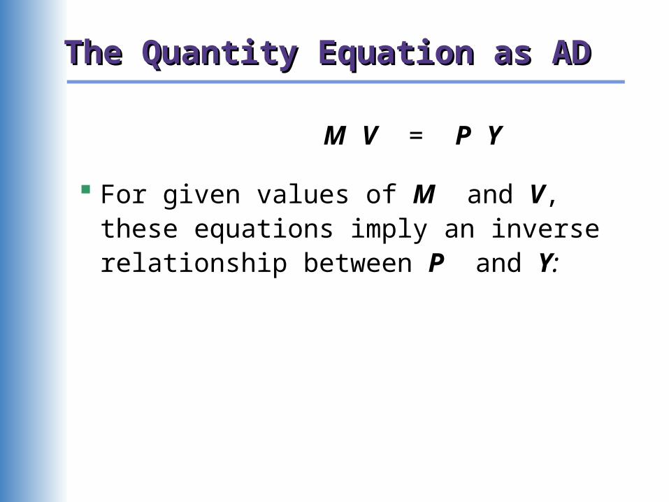
The Quantity Equation as ADThe Quantity Equation as AD
M V = P Y
For given values of M and V, these equations imply an inverse relationship between P and Y:

The downward-sloping The downward-sloping ADAD curve curve
An increase in the price level causes a fall in real money balances (M/P ),
causing a decrease in the demand for goods & services.
Y
P
AD
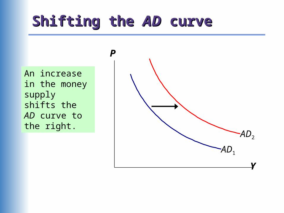
Shifting the Shifting the ADAD curve curve
An increase in the money supply shifts the AD curve to the right.
Y
P
AD1
AD2
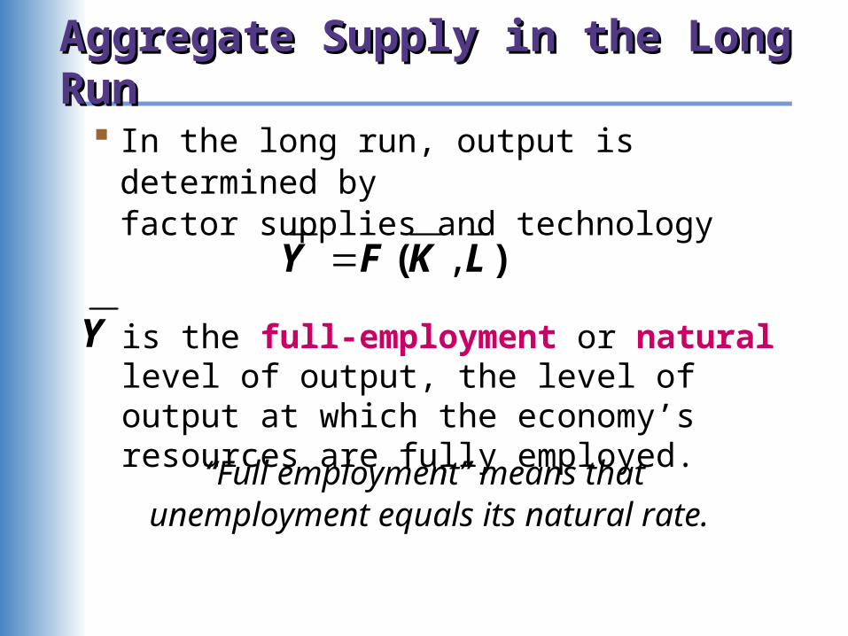
Aggregate Supply in the Long RunAggregate Supply in the Long Run
In the long run, output is determined by
factor supplies and technology, ( )Y F K L
is the full-employment or natural level of output, the level of output at which the economy’s resources are fully employed.
Y
“Full employment” means that unemployment equals its natural
rate.
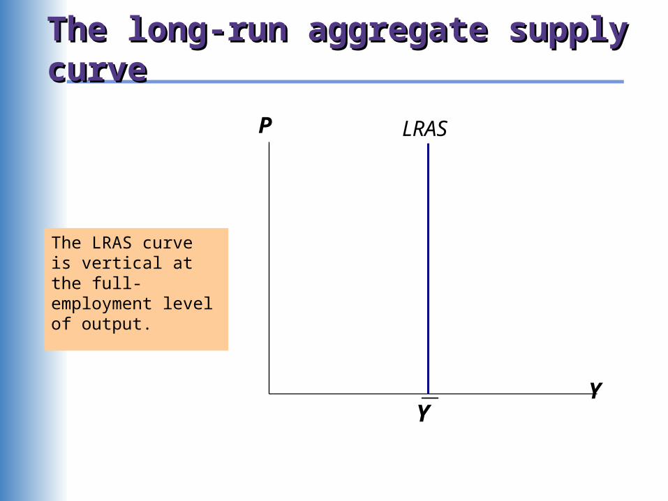
The long-run aggregate supply curveThe long-run aggregate supply curve
Y
P LRAS
Y
The LRAS curve is vertical at the full-employment level of output.
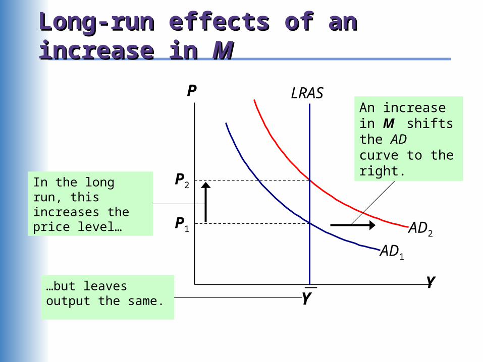
Long-run effects of an increase in Long-run effects of an increase in MM
Y
P
AD1
AD2
LRAS
Y
An increase in M shifts the AD curve to the right.
P1
P2In the long run, this increases the price level…
…but leaves output the same.
Aggregate Supply in the Short RunAggregate Supply in the Short Run
In the real world, many prices are sticky in the short run.
For now (and throughout Chapters 9-11), we assume that all prices are stuck at a predetermined level in the short run…
…and that firms are willing to sell as much at that price level as their customers are willing to buy.
Therefore, the short-run aggregate supply (SRAS) curve is horizontal:
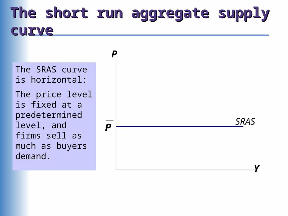
The short run aggregate supply curveThe short run aggregate supply curve
Y
P
PSRAS
The SRAS curve is horizontal:
The price level is fixed at a predetermined level, and firms sell as much as buyers demand.

Short-run effects of an increase in Short-run effects of an increase in MM
Y
P
AD1
AD2
…an increase in aggregate demand…
In the short run when prices are sticky,…
…causes output to rise.
PSRAS
Y2Y1
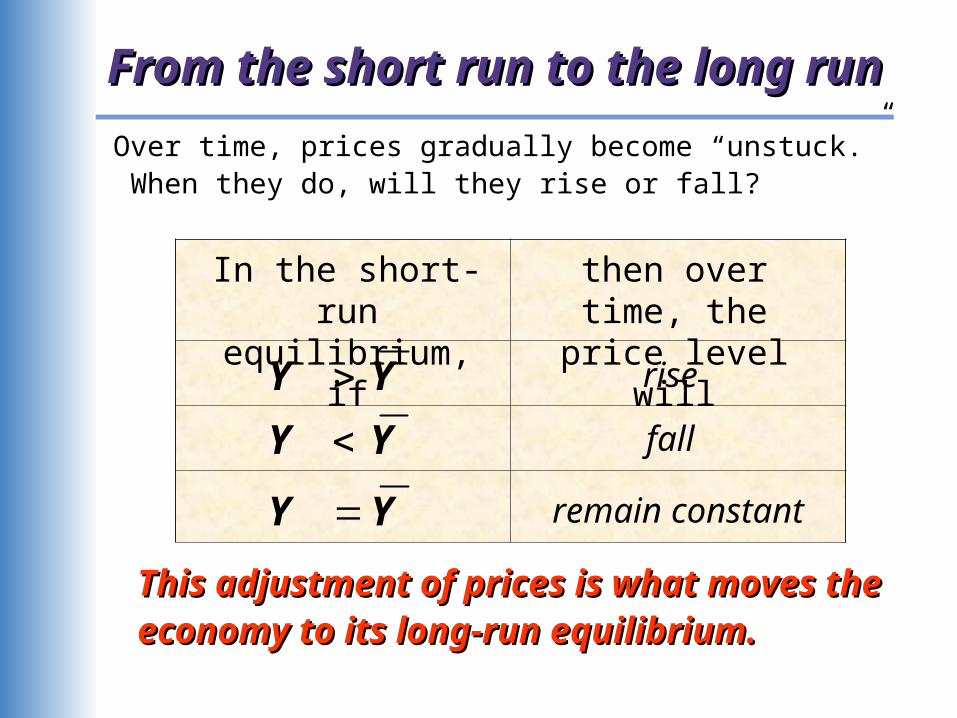
From the short run to the long runFrom the short run to the long run
Over time, prices gradually become “unstuck.” When they do, will they rise or fall?
Y Y
Y Y
Y Y
rise
fall
remain constant
In the short-run equilibrium, if
then over time, the price level
will
This adjustment of prices is what moves the This adjustment of prices is what moves the economy to its long-run equilibrium.economy to its long-run equilibrium.
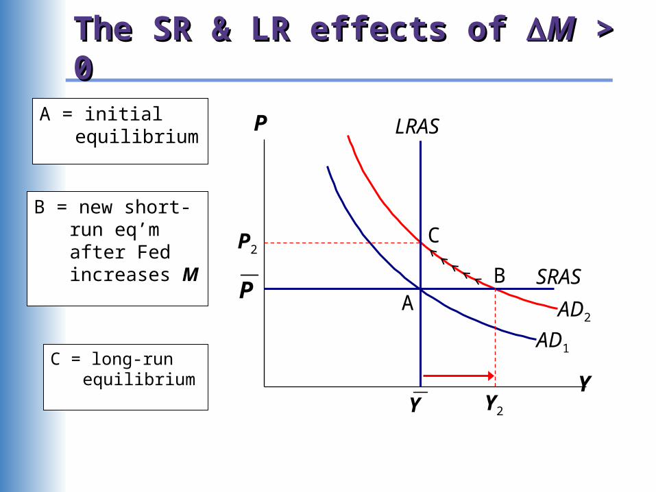
The SR & LR effects of The SR & LR effects of MM > 0 > 0
Y
P
AD1
AD2
LRAS
Y
PSRAS
P2
Y2
A = initial equilibrium
AB
CB = new short-
run eq’m after Fed increases M
C = long-run equilibrium
How shocking!!!How shocking!!!
shocks: exogenous changes in aggregate supply or demand
Shocks temporarily push the economy away from full-employment.
An example of a demand shock:exogenous decrease in velocity
If the money supply is held constant, then a decrease in V means people will be using their money in fewer transactions, causing a decrease in demand for goods and services:
LRAS
AD2
PSRAS
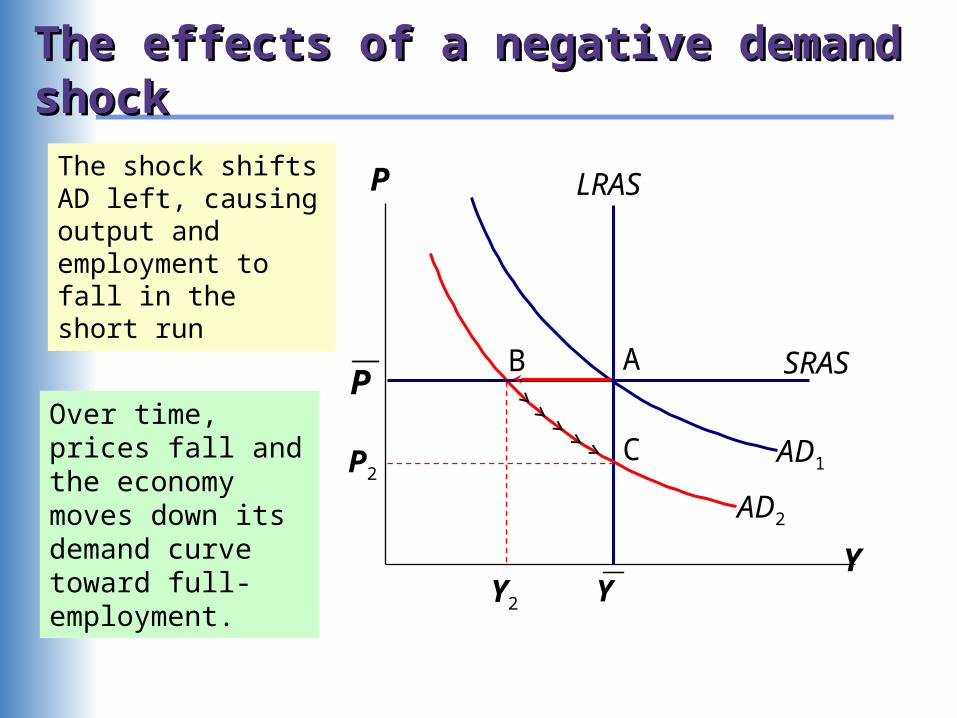
The effects of a negative demand shockThe effects of a negative demand shock
Y
P
AD1
Y
P2
Y2
The shock shifts AD left, causing output and employment to fall in the short run
AB
COver time, prices fall and the economy moves down its demand curve toward full-employment.
Supply shocksSupply shocks
A supply shock alters production costs, affects the prices that firms charge. (also called price shocks)
Examples of adverse supply shocks: Bad weather reduces crop yields, pushing up
food prices. Workers unionize, negotiate wage increases. New environmental regulations require firms
to reduce emissions. Firms charge higher prices to help cover the costs of compliance.
(Favorable supply shocks lower costs and prices.)
CASE STUDY: CASE STUDY: The 1970s oil shocksThe 1970s oil shocks
Early 1970s: OPEC coordinates a reduction in the supply of oil.
Oil prices rose11% in 1973 68% in 1974 16% in 1975
Such sharp oil price increases are supply shocks because they significantly impact production costs and prices.

1P SRAS1
Y
P
AD
LRAS
YY2
The oil price shock shifts SRAS up, causing output and employment to fall.
A
BIn absence of further price shocks, prices will fall over time and economy moves back toward full employment.
2P SRAS2
CASE STUDY: CASE STUDY: The 1970s oil shocksThe 1970s oil shocks
A

CASE STUDY: CASE STUDY: The 1970s oil shocksThe 1970s oil shocks
Predicted effects of the oil price shock:• inflation • output • unemployment
…and then a gradual recovery. 0%
10%
20%
30%
40%
50%
60%
70%
1973 1974 1975 1976 1977
4%
6%
8%
10%
12%
Change in oil prices (left scale)
Inflation rate-CPI (right scale)
Unemployment rate (right scale)
CASE STUDY: CASE STUDY: The 1970s oil shocksThe 1970s oil shocks
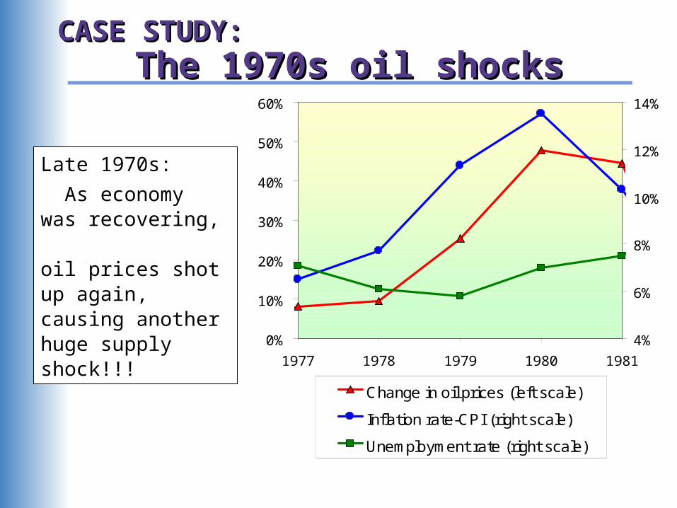
Late 1970s:
As economy was recovering, oil prices shot up again, causing another huge supply shock!!! 0%
10%
20%
30%
40%
50%
60%
1977 1978 1979 1980 1981
4%
6%
8%
10%
12%
14%
Change in oil prices (left scale)
Inflation rate-CPI (right scale)
Unemployment rate (right scale)

CASE STUDY: CASE STUDY: The 1980s oil shocksThe 1980s oil shocks
1980s: A favorable supply shock--a significant fall in oil prices.
As the model would predict, inflation and unemployment fell:
-50%
-40%
-30%
-20%
-10%
0%
10%
20%
30%
40%
1982 1983 1984 1985 1986 1987
0%
2%
4%
6%
8%
10%
Change in oil prices (left scale)
Inflation rate-CPI (right scale)
Unemployment rate (right scale)
Stabilization policyStabilization policy
def: policy actions aimed at reducing the severity of short-run economic fluctuations.
Example: Using monetary policy to combat the effects of adverse supply shocks:

Stabilizing output with Stabilizing output with monetary policymonetary policy
1P SRAS1
Y
P
AD1
B2P SRAS2
A
Y2
LRAS
Y
The adverse supply shock moves the economy to point B.
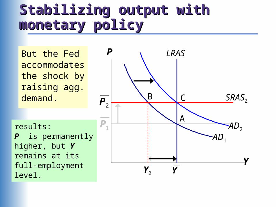
Stabilizing output with Stabilizing output with monetary policymonetary policy
1P
Y
P
AD1
B2P SRAS2
A
C
Y2
LRAS
Y
AD2
But the Fed accommodates the shock by raising agg. demand.
results: P is permanently higher, but Y remains at its full-employment level.

Chapter summaryChapter summary
1. Long run: prices are flexible, output and employment are always at their natural rates, and the classical theory applies.
Short run: prices are sticky, shocks can push output and employment away from their natural rates.
2. Aggregate demand and supply: a framework to analyze economic fluctuations

Chapter summaryChapter summary
3. The aggregate demand curve slopes downward.
4. The long-run aggregate supply curve is vertical, because output depends on technology and factor supplies, but not prices.
5. The short-run aggregate supply curve is horizontal, because prices are sticky at predetermined levels.

Chapter summaryChapter summary
6. Shocks to aggregate demand and supply cause fluctuations in GDP and employment in the short run.
7. The Fed can attempt to stabilize the economy with monetary policy.

Estimates of fiscal policy multipliersEstimates of fiscal policy multipliers
from the DRI macroeconometric model
Assumption about monetary policy
Estimated value of
Y / G
Fed holds nominal interest rate constant
Fed holds money supply constant
1.93
0.60
Estimated value of
Y / T
1.19
0.26

CASE STUDY: CASE STUDY:
The U.S. recession of 2001The U.S. recession of 2001 During 2001,
– 2.1 million people lost their jobs, as unemployment rose from 3.9% to 5.8%.
– GDP growth slowed to 0.8% (compared to 3.9% average annual growth during 1994-2000).
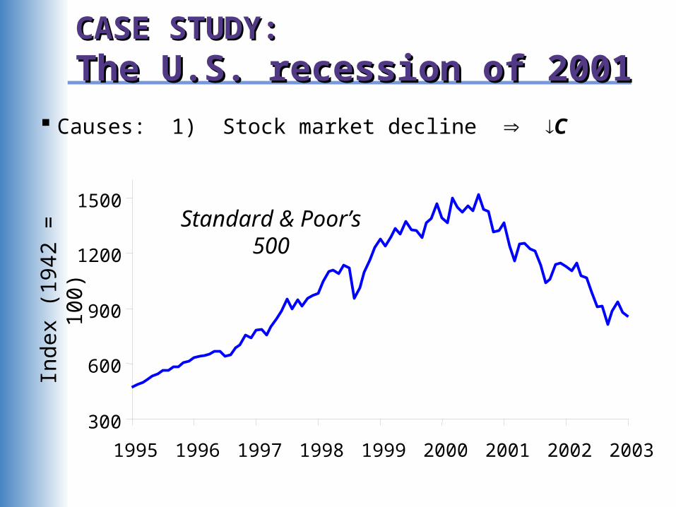
CASE STUDY: CASE STUDY:
The U.S. recession of 2001The U.S. recession of 2001
Causes: 1) Stock market decline C
300
600
900
1200
1500
1995 1996 1997 1998 1999 2000 2001 2002 2003
Ind
ex
(19
42
= 1
00
) Standard & Poor’s 500
CASE STUDY: CASE STUDY:
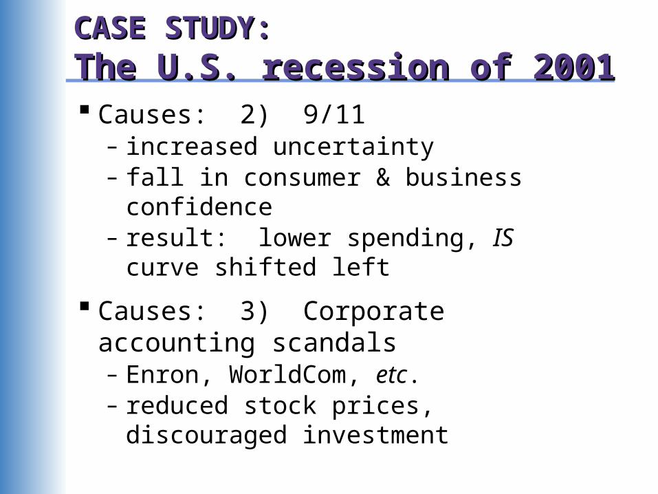
The U.S. recession of 2001The U.S. recession of 2001 Causes: 2) 9/11
– increased uncertainty– fall in consumer & business
confidence– result: lower spending, IS curve
shifted left
Causes: 3) Corporate accounting scandals– Enron, WorldCom, etc. – reduced stock prices, discouraged
investment

CASE STUDY: CASE STUDY:
The U.S. recession of 2001The U.S. recession of 2001 Fiscal policy response: shifted IS
curve right– tax cuts in 2001 and 2003– spending increases
•airline industry bailout•NYC reconstruction •Afghanistan war

CASE STUDY: CASE STUDY:
The U.S. recession of 2001The U.S. recession of 2001 Monetary policy response: shifted LM curve right
Three-month T-Bill Rate
Three-month T-Bill Rate
0
1
2
3
4
5
6
7
01/0
1/20
0004
/02/
2000
07/0
3/20
0010
/03/
2000
01/0
3/20
0104
/05/
2001
07/0
6/20
0110
/06/
2001
01/0
6/20
0204
/08/
2002
07/0
9/20
0210
/09/
2002
01/0
9/20
0304
/11/
2003
What is the Fed’s policy instrument?What is the Fed’s policy instrument?
The news media commonly report the Fed’s policy changes as interest rate changes, as if the Fed has direct control over market interest rates.
In fact, the Fed targets the federal funds rate – the interest rate banks charge one another on overnight loans.
The Fed changes the money supply and shifts the LM curve to achieve its target.
Other short-term rates typically move with the federal funds rate.
What is the Fed’s policy instrument?What is the Fed’s policy instrument?
Why does the Fed target interest rates instead of the money supply?
1) They are easier to measure than the money supply.
2) The Fed might believe that LM shocks are more prevalent than IS shocks. If so, then targeting the interest rate stabilizes income better than targeting the money supply. (Problem Set #16.)

The Great DepressionThe Great Depression
Unemployment (right scale)
Real GNP(left scale)
120
140
160
180
200
220
240
1929 1931 1933 1935 1937 1939
bill
ion
s o
f 19
58
do
llars
0
5
10
15
20
25
30
pe
rce
nt o
f la
bo
r fo
rce
THE SPENDING HYPOTHESIS: THE SPENDING HYPOTHESIS: Shocks to the Shocks to the ISIS curve curve
asserts that the Depression was largely due to an exogenous fall in the demand for goods & services – a leftward shift of the IS curve.
evidence: output and interest rates both fell, which is what a leftward IS shift would cause.

THE SPENDING HYPOTHESIS: THE SPENDING HYPOTHESIS: Reasons for the Reasons for the ISIS shift shift
Stock market crash exogenous C – Oct-Dec 1929: S&P 500 fell 17%– Oct 1929-Dec 1933: S&P 500 fell 71%
Drop in investment– “correction” after overbuilding in the 1920s– widespread bank failures made it harder to obtain
financing for investment
Contractionary fiscal policy– Politicians raised tax rates and cut spending to
combat increasing deficits.
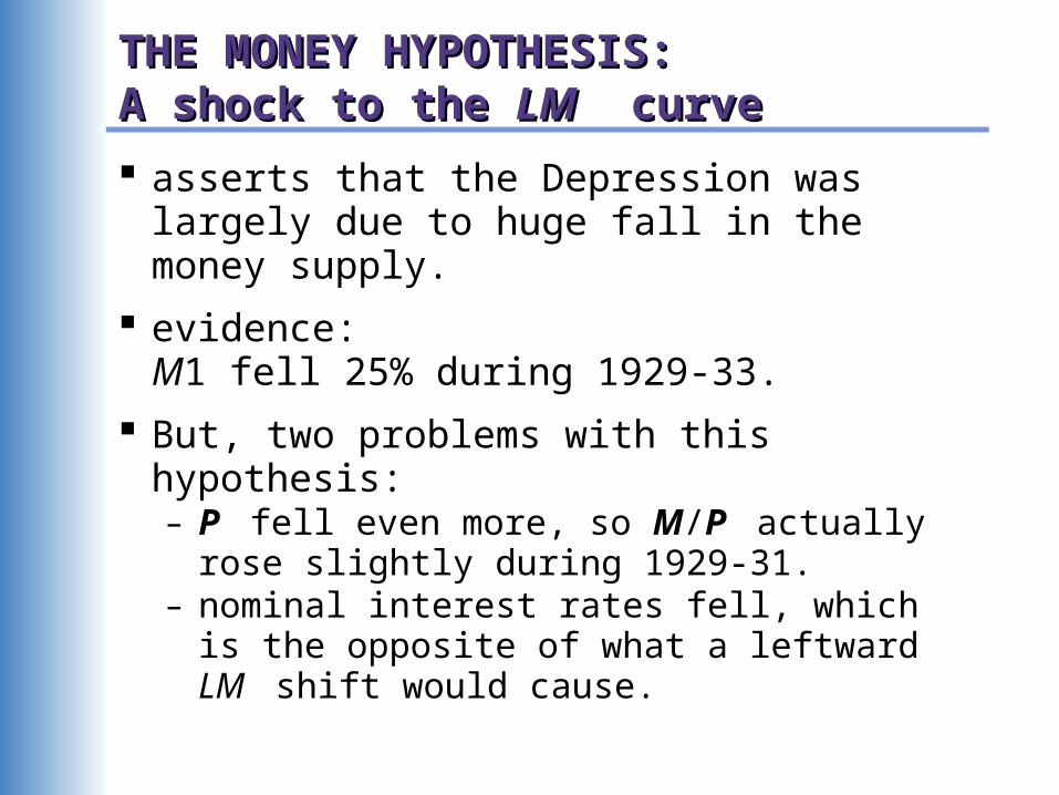
THE MONEY HYPOTHESIS: THE MONEY HYPOTHESIS: A shock to the A shock to the LMLM curve curve
asserts that the Depression was largely due to huge fall in the money supply.
evidence: M1 fell 25% during 1929-33.
But, two problems with this hypothesis:– P fell even more, so M/P actually rose
slightly during 1929-31. – nominal interest rates fell, which is the
opposite of what a leftward LM shift would cause.

THE MONEY HYPOTHESIS AGAIN: THE MONEY HYPOTHESIS AGAIN: The effects of falling pricesThe effects of falling prices
asserts that the severity of the Depression was due to a huge deflation:
P fell 25% during 1929-33.
This deflation was probably caused by the fall in M, so perhaps money played an important role after all.
In what ways does a deflation affect the economy?
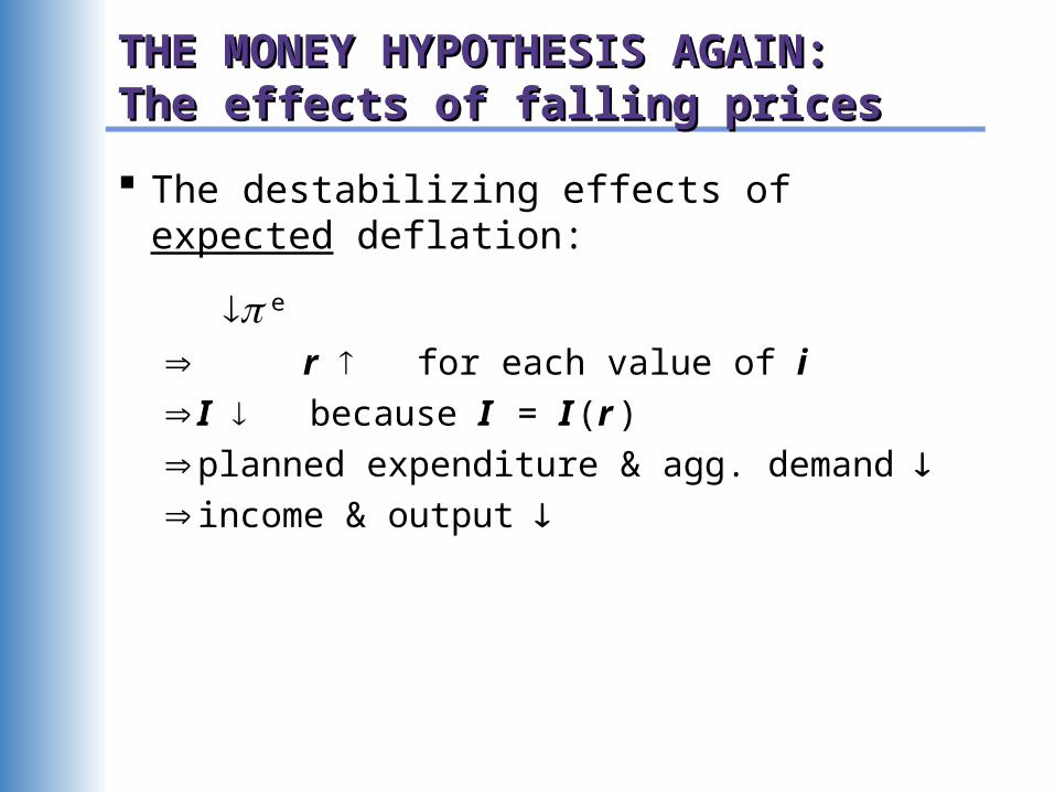
THE MONEY HYPOTHESIS AGAIN: THE MONEY HYPOTHESIS AGAIN: The effects of falling pricesThe effects of falling prices
The destabilizing effects of expected deflation:
e
r for each value of i I because I = I (r )planned expenditure & agg. demand income & output
Why another Depression is unlikelyWhy another Depression is unlikely
Policymakers (or their advisors) now know much more about macroeconomics:– The Fed knows better than to let M fall
so much, especially during a contraction.– Fiscal policymakers know better than to raise
taxes or cut spending during a contraction.
Federal deposit insurance makes widespread bank failures very unlikely.
Automatic stabilizers make fiscal policy expansionary during an economic downturn.