Macro-Financial Interactions in a Changing World

Eddie Gerba e.e.gerba@lse.ac.uk

DANMARKS NATIONALBANK

Danilo Leiva-Leon danilo.leiva@bde.es

BANCO DE ESPANA

The Working Papers of Danmarks Nationalbank describe research and development, often still ongoing, as a contribution to the professional debate.

The viewpoints and conclusions stated are the responsibility of the individual contributors, and do not necessarily reflect the views of Danmarks Nationalbank.

1 0 M AR C H 2 02 0 — N O . 15 3

W O R K I N G P A P E R — D A N M AR K S N A T IO N A L B A N K

1 0 M AR C H 2 0 2 0 — N O . 15 3

Abstract We measure the time-varying strength of macro-financial linkages within and across the US and euro area economies by relying on factor models with drifting parameters, where real and financial cycles are extracted and shocks are identified via sign and exclusion restrictions. The main results show that the euro area is disproportionately more sensitive to shocks in the US macroeconomy and financial sector, resulting in an asymmetric cross-border spillover pattern between the two economies. Moreover, while macro-financial interactions have steadily increased in the euro area since the late 1980s, they have oscillated in the US,, exhibiting very long cycles of macro- financial interdependence.

Resume Vi måler den varierende styrke af makrofinansielle sammenhænge over tid i og på tværs af den amerikanske økonomi og økonomien i euroområdet. Vi gør det på grundlag af faktormodeller med glidende parametre, hvorfra realøkonomiske og finansielle cyklusser uddrages, og stød identificeres via restriktioner på fortegn og eksklusionsrestriktioner. De vigtigste resultater viser, at euroområdet er uforholdsmæssigt mere følsomt over for stød i den amerikanske makroøkonomi og finansielle sektor, hvilket resulterer i asymmetriske grænseoverskridende effekter mellem de to økonomier. Endvidere ses det, at mens de makrofinansielle interaktioner er steget løbende i euroområdet siden slutningen af 1980’erne, har de i USA været forbundet med udsving i form af meget lange cyklusser med indbyrdes makrofinansiel afhængighed.

Macro-Financial Interactions in a Changing World

Acknowledgements We would like to thank the participants of the 2019 Bayesian Econometrics Workshop, 34th Annual Congress of the European Economic Association, 50th Annual Conference of the Money, Macro and Finance, Research (LSE), and the Research Seminar Series of Danmarks Nationalbank for helpful comments and suggestions.

The views expressed in this paper are those of the authors. No responsibility for them should be attributed to Danmarks Nationalbank, the Banco de Espana or the Eurosystem.

Key words Macro-financial linkages; Dynamic factor models; TVP-VAR.

JEL classification E44; C32; C55; F44; E32; F41.

Macro-Financial Interactions in a Changing World∗

Eddie Gerba† Danilo Leiva-Leon‡

Abstract

We measure the time-varying strength of macro-financial linkages within and across

the US and euro area economies by relying on factor models with drifting parameters,

where real and financial cycles are extracted and shocks are identified via sign and

exclusion restrictions. The main results show that the euro area is disproportionately

more sensitive to shocks in the US macroeconomy and financial sector, resulting in

an asymmetric cross-border spillover pattern between the two economies. Moreover,

while macro-financial interactions have steadily increased in the euro area since the

late 1980s, they have oscillated in the US,, exhibiting very long cycles of macro-

financial interdependence.

Keywords: Macro-financial linkages, dynamic factor models, TVP-VAR.

JEL codes: E44, C32, C55, F44, E32, F41.

∗We would like to thank the participants of the 2019 Bayesian Econometrics Workshop, 34th AnnualCongress of the European Economic Association, 50th Annual Conference of the Money, Macro and FinanceResearch (LSE), and the Research Seminar Series of Danmarks Nationalbank for helpful comments andsuggestions. The views expressed in this paper are those of the authors. No responsibility for them shouldbe attributed to Danmarks Nationalbank, the Banco de Espana or the Eurosystem.†Danmarks Nationalbank, Advisor, Havnegade 5, DK-1093 Copenhagen. Email: E.E.Gerba@lse.ac.uk‡Banco de Espana, ES-28014 Madrid. Email: danilo.leiva@bde.es

1 Introduction

The eagerness to understand macro-financial linkages has increased at an unprededented

rate in recent years. Much of this has been driven by the desire to comprehend the forces

that led to the Great Recession, including the deep and long-lasting consequences of the

financial downturn which began in 2007. In particular, recent research on macro-finance

has focused on the role of the financial sector as a generator of shocks which are transferred

to the overall economy via macro-financial linkages. Less (albeit some) effort has been

put into understanding how the macroeconomy can create and transmit shocks to the

financial sector. Moreover, very little effort has been invested in grasping the role that

linkages themselves may play as amplifier and feedback loop for shocks generated inside

the linkages as well as elsewhere. Yet, the prospect for a full recovery seems bleack at

present. Despite unprecedented monetary expansion and supportive fiscal policy, per-

capita income growth has stagnated in many jurisdictions, including the US and euro

area. Therefore, understanding how macro-financial interactions can condition a potential

recovery has become crucial for policymakers.

Figure 1 shows a diagram which illustrates the complexities embedded in macro-financial

interactions. Each economy in the figure has two sectors, the macroeconomic and the fi-

nancial. Domestic spillovers between the sectors in the US (euro area) are denoted by red

(blue) solid arrows. In parallel, cross-border interactions between the sectors are denoted

with dashed arrows. Moreover, all these relationships may be subject to potential funda-

mental changes over time for a number of reasons, opening an additional dimension to the

problem. One outcome from Figure 1 is that the study of international macro-financial

dynamic interactions, albeit crucial for policymakers, is challenging due to all the possible

ways in which shocks could be transmitted. The aim of this paper is to provide a robust

assessment of these interactions by taking all these underlying dimensions into account.

The first part of the problem involves defining what the macroeconomic and financial

cycles are. Yet, in the empirical literature there is still a wide debate over the exact defi-

nition of a real cycle and how different and more complete it is compared to the standard

business cycle. For the financial counterpart, there is even less consensus on what con-

stitutes a financial cycle, its statistical characterisation and how similar it is to the real

1

Figure 1: International macro-financial dynamic interactions

United States Euro Area

Financial

Macro

Financial

Macro

Note: Solid red (blue) arrows denote the domestic macro-financial interactions forthe US (euro area). Dashed red arrows make reference to the spillovers from the USto the euro area. Dashed blue arrows denote the spillovers from the euro area to theUS

cycle. The existing definitions usually tend to be narrow (normally incorporating just a few

variables in order to capture the multi-faceted nature of the real or financial sectors), ex-

ogenously pre-determined (constructed such that they reproduce pre-determined statistical

characteristics), or based on short time series samples.1

Recognising the above shortcomings, this paper attempts to provide a comprehensive

definition of real and financial cycles using dynamic factor models. Unlike previous studies,

our empirical framework allows for an endogenous and time-varying selection of variables

in the construction of each of the latent cycles, selecting from a large dataset of real

activity and financial indicators, for each economy. These variables include information

about output, employment, production, consumption, etc., on the real side and information

regarding balance sheets, credit, foreign financial activity, etc., on the financial side of the

economy. The motivation for including this feature in our modelling strategy is based

on the need for flexibility in the determination of the most relevant variables driving the

financial cycle over time, given the lack of consensus about its definition.

The second part of the problem consists of measuring the intensity of the evolving macro-

1Section 2 provides a detailed review of the literature on the study of macro-financial linkages.

2

financial interactions. To quantify the degree of time variation and profundity in linkages,

the cycles are allowed to endogenously evolve according to a structural VAR model with

drifting coefficients. The identification of real and financial structural shocks is based on

the use of exclusion, sign and timing restrictions on the impulse response functions, along

with alternative schemes for robustness. To the best of our knowledge, this is the first study

of macro-financial spillovers between the US and the euro area, each as single economic

units, that covers a period starting in the 1980s. In particular, the sample starts in 1981:II

for the case of the euro area, which is considerably longer than the sample analyzed in any

of the previous studies focusing on macro-financial linkages in this region. Equally, due to

good data availability, we can go as far back as 1960:I for the US.

Moreover, we measure the linkages between macroeconomic and financial conditions in

a number of ways in order to provide a comprehensive assessment. Besides the qualitative

comparison of the real and financial cycles, and the computation of their time-varying

correlation, we examine the mutual impact and propagation of structural shocks over time,

calculate the time-varying forecast error variance decomposition at different horizons to

assess the predictive power that one cycle has on another, and examine the time-varying

factor loadings for the real and the financial cycle to measure the strength of common

patterns inside each sector.

Lastly, the third part of the problem focuses on quantifying the intensity of cross-border

spillovers in the macro-financial sphere. In doing so, we propose a joint (two-economy)

model which basically nests the two single-economy models. Considering that US and the

euro area top the list of global GDP figures, it is of global relevance to understand their

dynamics and the cross-border propagation of shocks. Moreover, the topic is of high policy

relevance considering the recent attempts to bring the two economies closer by creating

special economic agreements (such as the TTIP), foster deeper financial cross-border flows

(global banks, EU passport in banking and market financing in euro area), and enforce

regulatory harmonisation (transatlantic mutual recognition of regulation on securities and

derivatives, Basel III and FSB).2

With longer and smoother financial cycles compared to the macroeconomic cycle, both

2= Transatlantic Trade and Investment Partnership

3

in the euro area and in the US, our results robustly uncover a number of highly policy-

relevant features about the evolution of international macro-financial interactions. First,

while the euro area has exhibited increasing commonalities in the financial sector since the

early 2000s, the strength of commonalities in the US financial sector has remained relatively

steady over time. In particular, euro area private sector liabilities have become increasingly

determinant for the shape and evolution of financial cycles. Second, while macro-financial

interactions have steadily increased in the euro area since the late 1980s, they have oscillated

in the US, exhibiting very long cycles of macro-financial interdependence. Moreover, the

integration of the financial sector into the overall economy and the increase in the interplay

between the two sectors has been more intense in the US, while being more solid and

gradual in the euro area. Third, we unveil significant differences in the transmission of

mutual shocks. In the euro area, the propagation of shocks has increased in both directions,

i.e. from financial to real, and real to financial, but in the US, it has only increased in the

first direction, from financial to real. Likewise, the degree of responsiveness of the financial

sector to macroeconomic shocks is comparatively higher in the US, suggesting a deeper

integration between the two sectors. Fourth, the intensity in the transmission of macro-

financial shocks across borders is highly asymmetric, mainly going from US to euro area. In

particular, there is a dimension of asymmetry whereby unexpected deteriorations in the US

economy are detrimental for euro area financial conditions, while unexpected deteriorations

in the euro area economy could be beneficial for the financial conditions in the US These

asymmetries increased over time, until the Great Recession.

The rest of the paper is organized as follows: Section 2 provides a brief review of

the literature that helps to identify our contributions. Section 3 describes the employed

empirical framework. Section 4 analyses domestic macro-financial linkages. Section 5

studies international spillovers. Section 6 provides our conclusions.

2 Literature review

The financial turmoil of 2008 sparked an interest in studying the structural interplay

between financial cycles and the broader economy. While the questions raised in those

4

studies were not necessarily new, and build on the arguments laid out in the 1930s and

1970s (Fisher (1933) and Minsky (1977)), the scope of the pre-Great Recession studies were

much narrower, focusing either on a few cycles, particular aspect, or a particular segment

of the financial sector. For instance, there were studies showing the procyclical nature of

the financial system (Borio et al. (2001) and Borio and Lowe (2002)). Others have tried to

find long-run regularities in financial crises and the factors leading up to them (Reinhart

and Rogoff (2009)).3

The recent empirical studies examining the interplay between macroeconomic and fi-

nancial cycles can generally be divided into two main strands. The first one focuses on the

measurement of both cycles, which presents challenges, especially when defining a financial

cycle. Conversely, the second strand focuses on assessing changes over time in the relation-

ship between macroeconomic and financial cycles. Next, we proceed to briefly review the

two strands of the literature to elucidate the contributions of this paper.

In the first place, studies that have focused on the measurement of the cycles can be

grouped into four categories. The first category uses frequency-based filters to extract the

cyclical components of macroeconomic and financial variables and to describe their similar-

ities and differences. Most of these studies find that financial cycles have a longer duration

and are larger in amplitude than business cycles, but with an increasing synchronisation

over time (Drehmann et al. (2012), Aikman et al. (2015), Gerba (2015), Schueler et al.

(2017) and Gerba et al. (2017b)). However, since these measures are not based on a

given theory or model, the analysis of their interdependence may return spurious results,

as shown in Phillips and Jin (2015).4 This is also the case for the second category, which

focuses on extracting cycles in frequency domain (Strohsal et al. (2015) and Schueller et al.

(2017)).5 An important shortcoming of this method is that, since it requires stationarity, it

makes it difficult to endogenously account for potential structural breaks, which may result

in a lengthening or shortening of the cycles. Third, a less restrictive way of depicting the

3In a recent work Jorda et al. (2017) document a set of historical features of macro-financial linkages,pointing to the prominent role that financial factors should have in macroeconomic models.

4Moreover, these studies either assume that the frequency between the two types of series is similar, orthat financial is ex ante longer than the business cycle.

5These studies also find that financial cycles, in general, are longer than real cycles, but show evidencefor both short- and medium-term cycles in real credit growth

5

two cycles is by relying on turning point identification by using the Bry-Boschan algorithm

(Harding and Pagan (2002), (2006)).6 The main drawback of this method is that it is exces-

sively agnostic and therefore also has very limited theory to explain the results. Fourth, to

overcome some of the drawbacks of non-parametric or agnostic filters, model-based filters

have been employed. This method is usually based on unobserved component models used

to extract cycles by relying on the Kalman filter (Galati et al. (2016) and Ruenster and

Vlekke (2016)).

In parallel, different empirical strategies have been employed to infer potential changes

in the relationship between macroeconomic and financial variables. The most employed

tool has been the vector autoregressions (VARs) subject to parameter instabilities. Blake

(2000) and Calza and Sousa (2006) use Threshold VAR models to measure the effect of

credit shocks on real activity for the US and euro area, respectively. Both studies show

evidence of a stronger impact occurring under low credit growth regimes. For similar

purposes, Davig and Hakkio (2010), Hubrich and Tetlow (2015) and Nason and Tallman

(2015) use Markov-switching VAR models to study the relationship between financial stress

and US economic activity.7 All these studies agree in that the propagation of financial

shocks to the real economy is different during high financial stress regime in comparison to

normal times.8 Other studies allow for instabilities in the VAR models that are smoother

than sudden changes of regimes i.e. by allowing parameters to evolve according to random

walks. For example, Prieto et al. (2016) use a time-varying parameter (TVP) VAR model

to analyse the contribution of credit spread shocks to the US economy. Gambetti and Musso

(2017) follow a similar approach to investigate the effect of credit supply shocks. Ciccarelli

et al. (2016) investigate commonalities and spillovers in macro-financial linkages by using

a panel VAR model with drifting coefficients.9 An important drawback of these studies is

that the employed measure of financial cycles is based on one or a few financial variables,

6As shown in Claessens et al. (2011) and Drehmann et al. (2012) financial cycles are also found to belonger than business cycles, although Cagliarini and Price (2017) don’t find sufficient evidence. Moreover,they find that business cycles display a higher degree of synchronisation with credit and house price cyclesthan with equity prices.

7Kaufmann and Valderrama (2010) apply a similar framework to also assess the case of the euro area.8In a recent work, Leiva-Leon et al. (2018) evaluate changes in the propagation of shocks between credit

sentiment and the macroeconomy by relying on a multivariate Markov-switching framework.9Also, Abbate et al. (2016) pursue a similar goal, but from an international perspective.

6

which usually are related to credit activity only. This is because of the computational

problems arising in estimating such models using a large number of variables. However,

this limitation precludes the estimation of a broad measure of the financial cycle, which is

a crucial feature given its complexity and the lack of consensus about its definition.

The two strands of the literature described above have been somehow disconnected.

This paper intends to unify them by, first, extracting both macroeconomic and financial

cycles from a large set of information using Kalman filtering techniques and second, casting

those extracted cycles into a structural VAR model with time-varying parameters to assess

changes in the propagation of their shocks. This modelling strategy, which consists of a

joint estimation (procedure described in Section 3 and Appendix A), allows us to infer

changes in macro-financial linkages from a robust and broader perspective than previous

studies. Additionally, we allow for a changing and flexible selection of variables driving

both the financial and the real cycle, and we identify real and financial shocks using a

strategy that is based on sign, exclusion and timing restrictions on the impulse response

functions.

We also incorporate an international dimension to our analysis by looking at cross-

border spillovers between the US and the euro area, both within the sectors and across.

In this regard, most of the studies have looked at the US outward spillover, finding that

US financial and real shocks matter significantly for the rest of the world. Using a struc-

tural VAR model for pre-2008 data, Bayami and Thahn Bui (2010) find that international

business cycles are largely driven by US financial shocks, with a minor role for shocks from

other advanced economies. Miranda-Agrippino and Rey (2018) equally find that there are

large financial spillovers from the US to the rest of the world.

Our framework is more extensive than previous studies since it allows us to identify

outward as well as inward spillovers in the US and the euro area, both within the sectors

as well as across them. Moreover, we allow the degree of spillover effects between the two

regions to exhibit potential changes over time. Therefore, we provide a full spectrum of

international macro-financial interactions, that is, across regions (US and euro area), across

sectors (macroeconomic and financial) and over time. The related literature is relatively

limited, and most of the related works assess the degree of financial crisis spillovers across

7

markets, without considering the cross-sectoral aspect (real economy) or the non-crisis

times.10

3 Empirical framework

This section describes the econometric framework used to jointly (i) extract macroeco-

nomic and financial cycles from large datasets and (ii) assess the evolving interdependence

between these cycles. Let Ft be a vector that contains nf indicators of financial conditions

and Rt be a vector containing nr indicators of real activity for a given economy. Our aim

is to provide a framework that allows for a flexible selection of the variables driving both

cycles over time and that also accounts for potential changes in the propagation of real and

financial shocks.

3.1 One-economy model

We rely on a dynamic factor model with drifting loadings and where the factors evolve

according to a VAR model with time-varying coefficients. Accordingly, consider the model

described in the following equations, Ft

Rt

=

Λf,t 0

0 Λr,t

ft

rt

+

vf,t

vr,t

, (1)

ft

rt

= Φ1,t

ft−1

rt−1

+ · · ·+ Φk,t

ft−k

rt−k

+

uf,t

ur,t

, (2)

where ft and rt denote the financial conditions and real activity factors, respectively.11

The idiosyncratic innovations, vt = (vf,t, vr,t)′, are assumed to be orthogonal between them

and normally distributed, vt ∼ N(0, diag(Ω)). The reduced form innovations from the

VAR, ut = (uf,t, ur,t)′, are also assumed to be normally distributed, ut ∼ N(0,Σ). To be

able to assess the propagation of real and financial shocks, we let ut = A−1εt, where the

10For instance, Gravelle et al. (2006) find evidence of shift-contagion across currency markets, but notbond markets. Dungey et al. (2010) find that the degree of shift-contagion depends on the crisis, withhigher levels during subprime US 2007 crises or the 1998 Russian/LTCM crisis.

11In the empirical applications, we assume k = 2.

8

vector εt = (εf,t, εr,t)′, denotes the underlying structural shocks, such that E(εtε

’t) = I,

and E(εtε’t−k) = 0, ∀k, and A denotes the impact multiplier matrix.

To allow for changes over time in the information contained in the cycles and in the

propagation of shocks between real and financial cycles, we let both the autoregressive

coefficients φt = vec(Φt), where Φt = [Φ1,t, ...,Φk,t], and the factor loadings λt = vec(Λt),

where Λt = [Λf,t,Λr,t]′, to be time-varying by following random walk dynamics,

φt = φt−1 +wt, (3)

λt = λt−1 + ωt. (4)

The innovations wt and ωt are white noise Gaussian processes with zero mean and constant

covariances, Ψw and Ψω, respectively.

To identify macroeconomic and financial shocks, previous studies have mainly relied on

a simple recursive, or Cholesky, identification strategy (Davig and Hakkio (2010), Hubrich

and Tetlow (2015), Nason and Tallman (2015), Abbate et al. (2016), Ciccarelli et al.

(2016), Prieto et al (2016)), which can be highly controversial. In a recent work, Gambetti

and Musso (2017) relied on the use of a large set of sign restrictions to identify loan

supply shocks. In this paper, we rely on a recent work by Arias et al. (2018) and use a

combination of a few sign, exclusion and timing restrictions to identify macroeconomic and

financial shocks. Additionally, we use an alternative identification strategy as a robustness

exercise, proposed by Bai and Wang (2015).

Regarding the strategy based on the combination of restrictions, we first assume that

real activity and financial conditions are persistent processes by assuming positive signs

in the off-diagonal entries of the impact multiplier matrix, A−1. Second, we assume that

positive real activity shocks have a positive contemporaneous effect on financial conditions,

but that a shock in financial conditions does not have a contemporaneous effect on real

activity. As noticed by Prieto et al. (2016) (and in many other studies), this assumption

implies that macroeconomic variables react to financial shocks with a delay, possibly be-

cause of wealth effects and other effects which involve financial intermediaries that take

time to materialise - in contrast to financial variables which may react instantaneously to

9

macroeconomic shocks. Third, consequently, we assume that it would take at least one

period for real activity to react to a shock in financial conditions. Therefore, we postulate

that a positive unexpected change in the financial cycle positively affects the real cycle

with a one period lag. This combination of restrictions is summarized in Table 1.

Table 1: Sign, exclusion and timing restrictions for the one-economy model

Financial Shock Real Shock

h=0Financial Cycle + +Real Cycle 0 +

h=1Financial Cycle ∗ ∗Real Cycle + ∗

Note: The symbol ∗ indicates that no restriction is imposed inthe corresponding relationship, and “h” denotes the horizon ofthe impulse response.

Bai and Wang (2015) proposed a way to perform structural analysis in a context of

dynamic factor models with factors that are governed by a vector autoregressive structure.

This identification strategy simply consists of directly restricting the variance-covariance

matrix of the reduced form innovations to be an identity matrix, i.e., Σ = I. Since the

variables in the VAR system are latent and jointly estimated with the rest of the param-

eters of the model, by imposing this restriction the rest of the elements in the model are

adjusted in such a way that the resulting innovations ut have a structural interpretation

by construction. As a robustness exercise, we alternatively employ this approach to assess

the propagation of shocks between macroeconomic and financial cycles. This information

corresponds to the solid arrows, red for US and blue for euro area, in Figure 1.

3.2 Two-economy model

The factor model described above is estimated for the two economies, US and euro area,

separately in order to provide a deep and accurate understanding of their corresponding

macro-financial linkages. However, we are also interested in identifying potential changes

in the cross-border spillovers between the two economies. In particular, we are interested

10

in estimating the time-varying effect of (i) financial shocks in the US to the financial cycle

in the euro area, (ii) real shocks in the US to the real cycle in the euro area, (iii) financial

shocks in the US to the real cycle in the euro area, (iv) real shocks in the US to the financial

cycle in the euro area, (v) financial shocks in the euro area to the financial cycle in the US,

(vi) real shocks in the euro area to the real cycle in the US, (vii) financial shocks in the

euro area to the real cycle in the US, and (viii) real shocks in the euro area to the financial

cycle in the US This information corresponds to the dashed arrows in Figure 1, red for

spillovers from US to the euro area, and blue for spillovers from euro area to US

In order to address these issues, we propose an extended, or joint, model that nests each

of the two models for individual economies. Accordingly, consider the following US-euro

area dynamic factor model:FUSt

RUSt

FEAt

REAt

=

ΛUS

f,t 0 0 0

0 ΛUSr,t 0 0

0 0 ΛEAf,t 0

0 0 0 ΛEAr,t

fUSt

rUSt

fEAt

rEAt

+

vUSf,t

vUSr,t

vEAf,t

vEAr,t

(5)

fUSt

rUSt

fEAt

rEAt

= Ψ1,t

fUSt−1

rUSt−1

fEAt−1

rEAt−1

+ · · ·+ Ψk,t

fUSt−k

rUSt−k

fEAt−k

rEAt−k

+

uUSr,t

uUSf,t

uEAr,t

uEAf,t

(6)

where FUSt and RUS

t denote the set of information on financial and real activity, respectively,

for the US economy. Similarly, FEAt and REA

t denote the same set of information but for

the euro area economy. Notice that, consequently, this joint model would extract four

latent factors associated to the financial and real cycles for the US (fUSt and rUS

t ) and for

the euro area (fEAt and rEA

t ). The main advantage of this joint model is that we allow

for the four latent factor to be endogenously interrelated in a VAR fashion. Moreover, we

also allow for time variation in the parameters of the VAR in order to identify changes

in the cross-border propagation of macroeconomic and financial shocks. The dynamics of

the evolving parameters are assumed to be of the same nature as the ones detailed in the

region-specific models, i.e. following independent random walks.

11

The reduced form innovations, u∗t = (uUSr,t , u

USf,t , u

EAr,t , u

EAf,t )′, and structural innovations,

ε∗t = (εUSr,t , ε

USf,t , ε

EAr,t , ε

EAf,t )′, are linked through the impact multiplier matrix, i.e. u∗t =

B−1ε∗t . The main challenge associated to the joint model arises when defining the restric-

tions to identify cross-border spillovers. As noticed by Prieto et al. (2016), structural

(DSGE) models are still not available in a form to derive meaningful and widely accepted

sign restrictions to disentangle real and financial shocks (see Eickmeier and Ng (2011) for

a discussion). However, we take advantage of the fact that the model incorporates two

economies instead of only one in order to define a set of restrictions that helps us to iden-

tify the underlying structural shocks. In particular, we assume that, within each region,

there is a positive and contemporaneous response of real activity and financial conditions

to both real and financial shocks. Next, we assume that euro area developments in general

have no contemporaneous impact on US developments, with only one exception: We allow

for the possibility that the financial conditions in the US and euro area contemporaneously

influence each other. Finally, we assume that positive US real shocks are favorable for

both real and financial conditions in the euro area. However, a positive financial shock in

the US would take at least one period to generate a positive influence on the euro area

macroeconomic conditions. This set of restrictions can be summarized in Table 2.

Table 2: Sign and exclusion restrictions for the two-economy model

Fin. Shock EA Real Shock EA Fin. Shock US Real Shock US

Financial Cycle EA + + ∗ +Real Cycle EA + + 0 +Financial Cycle US ∗ 0 + +Real Cycle US 0 0 + +

Note: The symbol ∗ indicates that no restriction is imposed on the corresponding relationship.

For robustness purposes, we additionally estimate the model by assuming an alterna-

tive shock identification strategy, which consists of a Cholesky factorization in Table 5 in

Appendix A.2. In doing so, we assume the following order of the latent factors. We order

first the US real cycle followed by the US financial cycle and by the real cycle of the euro

area, leaving at the end the financial cycle of the euro area. Notice that this order implies

that (i) financial shocks take at least one period to affect macroeconomic conditions and

12

(ii) US developments could contemporaneously affect euro area developments, but not vice

versa.

For further validation purposes, we re-estimate the model using a mixture of recursive

and sign restrictions as outlined in Table 6 of Appendix A.2. This consists of three parts:

(i) recursive restrictions within each block; (ii) euro area shocks do not contemporaneously

impact the US; (iii) leaving unrestricted the effects that US shocks have on euro area.

This is an alternative scheme that is sufficiently broad to incorporate the empirical results

contained in the current international macro-financial literature.

The overall output retrieved by the models described in this section provides a compre-

hensive analysis of macro-financial interactions along the following dimensions: (i) within

sectors of a given economy, (ii) across sectors within a given economy, (iii) across sectors

and across economies, and (iv) over the time dimension. Moreover, we provide a series of

additional exercises for robustness purposes, altering the estimation method of the latent

cycles, the identification of structural shocks, and potential changes in the volatility of

macroeconomic and financial cycles.

4 Macro-financial linkages

This section provides a comprehensive overview of the time-varying interactions between

macroeconomic and financial sectors, for the US and euro area. In doing so, we provide

different pieces of information designed to study these interactions from various perspec-

tives, for each economy separately. First, we assess the evolving strength of commonalities

within each of the two sectors, i.e. macroeconomic and financial. This is done by jointly

characterising the underlying cycles and inferring the segments of the real and financial

sectors that are most important for driving those cycles over time. Second, we provide

a characterisation of the joint propagation of macroeconomic and financial shocks. This

is performed by examining the time-varying correlation between the cycles and analysing

information contained in impulse responses and forecast error variance decompositions. We

aim to provide a discussion that is comparative in nature; consequently, the description of

the results is structured per type of feature, and not per economy. Notice that in the analy-

13

sis, we use the terms linkages and interactions intercheangably, treating them as synonyms

for deep and dynamically evolving relations between the two sectors. This is in contrast

to the commonly used word nexus or link which we interpret as not profoundly changing

over time.

4.1 Data

The description of the variables for the US economy is reported in Table 3 and was

retrieved from the St.Louis Fed database. The sample spans from 1960:I until 2017:IV,

covering four very distinct episodes in US contemporaneous economic history, including

the Golden Age, stagflation and oil shocks, Great Moderation and the Great Recession.

The list of variables used in the analysis of the euro area is reported in Table 4. The data

spans the period between 1980:I and 2014:IV, covering the pre-Single Market episode, as

well as the Single Market and the monetary union era. The data is gathered from the

work of Gerba et al. (2018a), in turn collected from a variety of international sources. One

set of variables comes from the ECB’s Euro Area-Wide Model including variables F1-F3,

F9-F11, R1-R5 in Table 4. Variables F4-F7 come from Datastream, while F8 and R6-R7

come from the OECD World Economic Outlook. The remaining variables are retrieved

from two BIS sources: F12-F19 and R8 from BIS Market data and F20-F21 from BIS

International Financial Statistics database. For the pre-EMU period, the series has been

backward extrapolated using weights from euro area-12 and then adjusted as the new

members joined the monetary union. Thus, the country weights for the pre-euro area

period reflect the relative economic strength of the member states in the union around the

time of the introduction of the physical euro coins in 2002.

All variables, except for ratios and spreads, are expressed in growth rates in our model.

Financial ratios and spreads are expressed in levels. Our data sample is extensive and

wide-ranging enough to encompass many aspects of the financial and real sectors. On the

financial side, we have included price as well as quantity variables. Price variables include

corporate financing spreads, financial ratios of firms and stock market indices. Quantities

include assets and liabilities of banks (including their subcomponents), assets and liabilities

of households and firms (along with their subcomponents), credit, monetary system net

14

foreign assets and liabilities, monetary aggregates and velocity of money. On the real

side, our sample comprises of aggregate as well as disaggregate macroeconomic measures.

Included are GDP and its aggregate demand components, labour market indicators and

variables capturing productivity and the supply side of the economy, such as real output

per hour, unit labor costs and compensation to employees.

4.2 Strength of commonalities within sectors

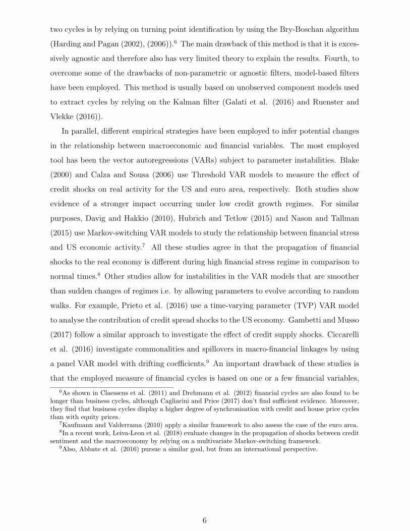
The estimated real and financial cycles of the US are plotted in Figure 2. It shows that

the financial cycle lasts much longer than the macroeconomic one. While financial activity

underwent two major contractions during our sample period (1992 and 2008), macroeco-

nomic activity experienced many more (albeit shorter) downturns. The first corresponds

to the global economic downturn in the Western world in the early 1990s, including the US

savings and loan crisis and a restrictive monetary policy. The second date corresponds to

the onset of the Great Recession. Also, the dynamics of the financial cycle are smoother

than those of the real one, experiencing much less of the very short-run variation. More-

over, the financial cycle experienced a profound change in frequency around 1990. While

the average length of a financial cycle was 5-7 years in the pre-1990 sample, it increased to

7-10 years in the subsequent period. The macroeconomic cycle, on the other hand, has an

average length of 2-5 years throughout the entire sample period.12

These attributes also apply to the euro area cycles, as can be seen from Figure 3.

Although the frequency of the financial cycle is again lower, there are some differences with

respect to the US case. While in the first half of the sample (1980-1996), the financial cycle

is largely below the trend, the real cycle had completed a full phase by that time. Also,

while the first boom phase in the financial cycle lasted for around 7 years (1996-2003), that

of the macroeconomy was 2 years shorter. It is also important to notice that there is a

stronger co-movement between both cycles starting from mid-1990s, with boom and bust

phases roughly coinciding, although the timing and magnitude are not entirely identical.

On the whole, there are significant differences in the nature of the two cycles. Financial

12In line with the Great Moderation literature, documented by McConnell and Perez-Quiros (2000),there has been a decline in the volatility of the real cycle since the mid-1980s.

15

cycles are longer and smoother, in particular since the 1990s, while real cycles have lower

amplitude and are more erratic. Also, it seems that higher and longer build-ups in the

financial sector have resulted in higher peaks, while more frequent reversals in the real

economy have resulted in deeper troughs for the macroeconomic cycle, relatively speak-

ing. Additionally, there seems to be a significant co-movement between the two cycles, in

particular for the euro area. The next section explores this feature in further detail. For

robustness purposes, we also compute the underlying cycles using principal components

(PC) and plot them in Figures 17 and 18 in the Appendix. Although PC provide a con-

sistent estimation of the factors, this method is not able to endogenously assess potential

instabilities in factor loadings. The results show that the factors estimated by PC follow a

similar pattern to the factors estimated with Bayesian methods, with the latter exhibiting

smoother and more stable dynamics, confirming our inferences about the two cycles.

Compared to alternative composite measures of financial activity, such as the National

Financial Conditions Index (NFCI) of Brave and Butters (2012),or the non-financial and

credit-to-GDP cycles, we find similarity to the non-financial leverage cycle. The long cycles

and the long buil-ups in particular since the 1990s are visible in both. However, the reversals

are sharper in our financial cycle, and the flexibility in our framework allows for long-term

movement in the trend, in parallel. In addition, like the leverage cycle, our financial cycle

is a good lead indicator and can serve as an early warning signal for financial stress and its

potential impact on economic growth. The swings in the cycle anticipate those of credit-

to-GDP and the business cycle (see Figure 4). In comparison to the adjusted NFCI, the

information contained in our financial cycle is more informative on the particular phase

of the cycle and the probability and severity of a subsequent reversal. The NFCI, on the

other hand, is better suited for risk monitoring and analysis of risk build-up.

We proceed to assess the durability in commonalities within each sector, defined as the

contemporaneous relationship between real and financial indicators with its corresponding

cycle (or factor). This evolving relationship is measured by the time-varying factor loadings.

The information is useful to identify potential changes in the composition of both cycles,

and therefore to interpret them in a more accurate manner.

For the US case, the dynamic correlation between the indicators (loadings) and cycles

16

is plotted in Figure 12. For the financial loadings, marked with F, and the macroeconomic

loadings, marked with R, a couple of features deserve to be mentioned. First, most of the

factor loadings associated to financial indicators are sizeable and statistically significant

over time, validating the underlying pattern of commonalities across different segments

of the financial sector. This is also the case for the loadings associated with real activity.

Second, with only a few exceptions, the degree of variability over time in the factor loadings

has remained relatively stable for both types of indicators. This result indicates that the

composition of US real and financial cycles has, in general, remained relatively unchanged.

The case of the euro area is somewhat different. Figure 13 plots the evolving rela-

tionship between indicators (loadings) and the cycle, F for the financial,and R for the

macroeconomic (or real). The results indicate a clear change in the composition of the

euro area financial cycle. On the one hand, indicators containing information about credit

and balance sheet variables have increased their correlation with the financial cycle over

time. This includes variables such as loans to non-banks by deposit institutions, loans to

non-governmental sector and monetary aggregates, but also others such as net foreign as-

sets and net foreign liabilities. Conversely, other sets of financial indicators have exhibited

a decreasing correlation with the financial cycle over time. These variables contain infor-

mation about the financial position of firms, such as price-earning ratios of non-financial

firms or price-book ratios of financial firms. Regarding the real sector, commonalities have

remained relatively steady. It is important to notice that the increasing convergence of

most of the variables with the financial cycle is significantly larger than the decoupling

exhibited by a few other financial variables, pointing to overall increasing commonalities

in the financial sector.

These features point to our first main result: Patterns in macro-financial linkages be-

tween the two economies are diverging. The euro area has exhibited increasing commonali-

ties in the financial sector since the early 2000s. On the other hand, the strength of the US

financial sector has remained relatively steady over time. Despite those divergences, there

are also similarities between the two economies. Macroeconomic indicators have exhibited a

relatively stable importance in shaping the real cycle. Furthermore, balance sheet (stocks)

and credit variables that have become more relevant in shaping the financial cycles can be

17

grouped into the liability side of the non-financial sector. In other words, private sector

liabilities have become increasingly determinant for the shape and evolution of financial

cycles.

4.3 Depth of linkages across sectors

This section focuses on measuring the evolving interaction between macroeconomic and

financial cycles from different perspectives to provide robust assessments. We start by

computing the time-varying correlation between the two cycles for each economy.13 For

the case of the US that correlation has varied significantly over time, as shown in Figure

8. In particular, between 1963 and 1992 the correlation consistently declined and reached

a record low of 0.4. Yet, this lost ground over 30 years was quickly recovered during the

subsequent period, and by 2009 the correlation was at a historical peak of above 0.67.

The growth rate in the correlation during 1990s and 2000s was more than twice as high

as the rate of decline in the previous episode. This particular period was characterized

by heavy deregulation in the US financial system, both across activities/segments and ge-

ographically. Also an intense financial deepening involving many of the known financial

innovations occurred during this period. As a result, competition between financial in-

stitutions intensified. The US financial system opened up heavily during this period and

attracted a lot of foreign capital. That capital fuelled two market bubbles: first in the

corporate financing market (dot-com boom) and then in the housing market (subprime).

On the real side, during this time inflation was significantly reduced and there was seem-

ingly stable and moderate growth. Apart from a very brief downturn in early 1990s and

the early 2000s, the rest of these two decades was characterised by a solid expansion. The

increased liquidity in the system also led to increased consumption and investment, and

solid employment and productivity figures. These changes potentially explain the rapid

increase in correlation between the two cycles over this period.

Next, when one also takes into account that the Great Recession, characterised by a

13Since the cycles, proxied by the factors, evolve according to a vector autoregression, we computethe unconditional variance-covariance matrix of the elements in the VAR, i.e. ft and rt, and not of itsinnovations. Next, we compute the corresponding correlation coefficient. Since this measure is only afunction of the parameters of the VAR, the same procedure is applied for each period of time to obtainthe desired time-varying correlation.

18

reversal in financial sector activity, outflow of capital, inflation volatility and weak growth,

interrupted this trend and led to a decline in the correlation between the two types of cycles

(down to 0.5 at the end of 2017).

The corresponding time-varying correlation for the euro area has behaved somewhat

differently. Figure 9 indicates that macro-financial interactions have continuously risen,

with the exception of the pre-Maastricht Treaty period between 1984-1991. After the

Single European Act in 1987, the correlation started to steadily grow, surpassing a historical

record of 0.7 by 2011. Notice that the collapse of the European Stability Mechanism in

1992 did not interrupt this long-term trend of macro-financial deepening. In general, since

the formal adoption of the euro, the correlation has grown slower compared to the previous

growth phase. These results indicate that the establishment of the Economic and Monetary

Union (EMU) and the adoption of the currency are associated with long-lasting stronger

interactions between the financial sector and the real economy.

Altogether, the correlation between the macroeconomic and financial cycles is high in

both economies, albeit with different time patterns. Our second main result shows that,

while macro-financial interactions have steadily increased in the euro area since the late

1980s, they have oscillated in the US around a mean of approximately 0.5, exhibiting

very long cycles of macro-financial interdependence. Additionally, over the past 25 years,

the correlation coefficient has been higher in the euro area, while the rate of change of

the correlation has been much larger in the US This implies that the integration of the

financial sector into the overall economy and the increase in the interplay between the two

have been more intense in the US, while more solid and gradual in the euro area.

We perform two types of robustness exercises associated with the vector autoregression

that provide further basis for measurement of macro-financial interactions. First, instead

of identifying the structural shocks using the baseline scheme, i.e. by imposing sign, ex-

clusion and timing restrictions on the impulse responses, we directly estimate orthogonal

innovations in the VAR, as in Bai and Wang (2015). The time-varying correlation between

macroeconomic and financial cycles based on orthogonal innovations is plotted in Figure

19 for the US, and in Figure 20 for the euro area, in Appendix A.3. The results show es-

timates that are qualitatively similar to the ones obtained with the baseline identification

19

scheme, providing robustness to our assessments. Second, for the case of the US, we also

account for the Great Moderation episode by imposing a break in the variance-covariance

matrix of the VAR innovations in 1985 in the baseline scheme. Figure 21 plots the time-

varying correlation, again showing qualitatively similar dynamics. However, notice that

the inclusion of the break in volatility is associated with an overall decline in the strength

of macro-financial linkages.

Next, we turn to potential changes over time in the propagation of real and financial

shocks for both economies. The top chart of Figure 10 plots the response of real activity to

a financial shock in a three-dimensional graph, while the bottom chart plots the response of

financial conditions to a real shock for the US economy. The results show a couple of salient

asymmetric patterns. First, while the sensitivity of financial conditions to real shocks has

remained relatively unchanged over time, the sensitivity of real activity to financial shocks

started to increase in the early 2000s. This finding explains the substantial deterioration of

the macroeconomy as a result of the financial shocks of the Great Recession between 2007

and 2009. Second, the effects of real shocks on financial conditions lasted significantly longer

than the effects of financial shocks on real activity. These patterns are more visible in the

two-dimensional graphs of dissected impulse responses, which are reported in Appendix A.3

to conserve space. Figure 22 plots the time-varying cumulated responses at pre-determined

horizons, showing that, in general, the effects of real shocks are not only larger, but also

more variable over time compared to financial shocks.

The transmission of shocks in the euro area, shown in Figure 11, presents a couple of

important differences when comparing it with the case of US First, the effect of financial

shocks on real activity has also increased over time. However, the increase started much

earlier than in the US, in particular since the early 1990s. Also, notice that around that

time financial conditions in the euro area also started to become more sensitive to real

shocks. These features are consistent with the sustained increase in synchronisation be-

tween macroeconomic and financial euro cycles shown in Figure 9. Second, the sensitivity

of real activity to financial shocks in the euro area is small on impact but long-lasting,

while in the US that sensitivity is large on impact but short-lasting, in relative terms.

These features can be seen in detail in the dissected impulse responses plotted in Figure 23

20

in Appendix A.3. Also, notice that the response which has exhibited the largest variation

over time is the one regarding the effects of real shocks on financial conditions.

Accordingly, our third main finding unveils asymmetric shock propagation patterns in

both economies. In the euro area, the interactions have increased in both directions, from

financial to real and vice versa, but in the US, they have increased in only one direction, from

financial to real. Also, the financial sector of the US shows a sensitivity to macroeconomic

shocks which is of higher magnitude and of shorter duration than in the euro area. These

asymmetries in macro-financial linkages remain even when we change the identification

scheme of structural shocks by directly assuming orthogonality in the innovations of the

VAR equation, see Figure 24, for the US and Figure 25, for the euro area in Appendix A.3.

These results persist even when we assume a break in volatility of the US economy in

1985. However, some features deserve commenting. Figure 26 shows that the Great Mod-

eration period is associated with a slight increase in responsiveness of the macroeconomy

to financial shocks, but also with a substantial reduction in the sensitivity of the financial

sector to real shocks. This implies that when the structural reduction in business cycle

fluctuations took place, real shocks not only became smaller but their ability to influence

financial conditions also diminished.

Next, we focus on measuring the predictive ability that developments in one sector,

i.e. macroeconomic or financial, may have on the other. In doing so, we follow the line

of Diebold and Yilmaz (2009) and rely on the notion of the Forecast Error Variance De-

composition (FEVD) obtained from the VAR equation of the model.14 We report the

corresponding results in Appendix A.3 for the sake of space. Figure 27 plots the FEVD

over time for the US economy showing that, in general, there have been no significant

changes in the contribution of shocks in one sector to future developments of the other,

with one important exception. Since the Great Recession, the information contained in

financial conditions increased its ability to predict future short-term developments of the

macroeconomy, as can be seen in the left plot of chart (b) in Figure 27. For the case of the

14A recent literature (Cotter et al (2017) and Korobilis and Yilmaz (2018), among others) focuses on usingthe network approach proposed in Diebold and Yilmaz (2009) to measure the degree of interconnectednessbetween international financial market segments (equity, sovereign credit, financial firms). These papersdo, however focus on other aspects of interest, such as networks, market monitoring, index performanceevaluations and non-structural volatility.

21

euro area, the situation is rather different. Since the early 1990s, real activity dynamics

started to increase their ability to predict future long-term developments in the financial

conditions, as shown in chart (c) of Figure 28. Also around that time, euro area financial

conditions started to become less predictable based on its own past dynamics.

5 International spillovers

Once we have defined the time-varying macro-financial interactions within an economy,

we proceed to examine the intensity of cross-border spillovers between the two economies,

both across the sectors and between them. As indicated by the dashed arrows in Figure

1, there are eight possible ways to consider cross-border interactions in macro-finance.

These different dimensions of spillovers are measured with the ‘global’ two-economy model,

described in Section 3.2. The estimated factors obtained with the two-economy model

follow similar patterns as the ones associated with the one-economy model, as can be seen

in Figure 29 in Appendix A.3. This provides additional robustness for our measurement of

both types of cycles.

First, we compute the cross-border and cross-sector time-varying correlations and report

them in Figure 14. The figure shows clear patterns associated with gradual, but sustained,

increases in the correlation between (i) US and euro area financial activity, (ii) US and

euro area real activity, and (iii) US financial and euro area real activity. Such an increasing

interdependence pattern persisted until the end of the Great Recession, and slightly declined

afterwards. The only exception is the correlation between the US real and euro area

financial activity, which has remained fairly stable over time.15

Although correlation measures are useful to address the overall strength of bilateral

cross-border macro-financial relationships, they remain silent about the asymmetric effects

between sectors and economies. Therefore, we proceed to evaluate the impulse response

functions retrieved from the two-economy model. Figure 15 shows the effect that shocks

generated in the US economy have on the euro area, while Figure 16 shows how shocks

15Notice that the two-economy model also delivers the time-varying correlations associated with sectorswithin a given economy. Such estimated correlations are qualitatively similar to the ones obtained withthe one-economy model, as can be seen in Figure 30 in Appendix A.3.

22

generated in the euro area could affect the US economy. The shocks are identified by

relying on the combination of sign and exclusion restrictions reported in Table 2. A clear

pattern emerges from the estimated joint model. The impact of US shocks is much larger

than the one associated with shocks coming from euro area. Real as well as financial shocks

originating from the US have a statistically and economically significant impact on euro

area macroeconomic and financial cycles, as can be seen in the dissected impulse responses

shown in Figure 31 in Appendix A.3.16 Notice that the largest increase over time is the

one of US real activity on E.A. financial conditions. Conversely, shocks from the euro

area tend to produce either small or short-lasting effects on the U.S economy (in line with

Jensen (2019)). In particular, real euro area shocks have an effect on US real activity that

only lasts one quarter. Also, the point estimates responses show that when the financial

or real conditions deteriorate (improve) in the euro area, the financial conditions in the

US improve (deteriorate). However, as shown in Figure 32 in Appendix A.3, this negative

impact is estimated with substantial uncertainty.

It is important to notice that the intensity in the transmission of shocks increases over

time, at least until the Great Recession. This is consistent with the increasing correlation

pattern between the factor across sectors and regions, shown in Figure 14. Also, there seems

to be no evidence of an intensification in the transmission of euro area shocks to the US since

the formal introduction of the Euro, at least not as a clearly visible change in pattern since

2000. These results suggest that the hegemony of the US in the international monetary and

financial system has been highly dominant (and increasing over time). The introduction

of the euro did not manage to alter this (in line with the discussion in Gourinchas et al.

(2019)).

There is, however, a subtle but important change in the transmission to euro area

financial conditions over 2000s. In particular, after around 2002, the transmission of shocks

arriving from the US seems to weaken somewhat, having persistently risen previously.

Even if this is not enough evidence to establish a causal relation, it coincides with the full

introduction of the euro on 1 January 2002. Hence, although the monetary union may not

16This finding is in line with the findings of Berg and Vu (2019) and Kose et al. (2017), who find eco-nomically and statistically significant effects on the world economy from US financial volatility. Giorgiadis(2016) finds similar results for US conventional and unconventional monetary policy.

23

have resulted in an increase in cross-border spillovers of real or financial activity, it seems

to have somewhat weakened the transmission of US shocks by creating a tighter net and

core, at least in the financial sphere.

Another relevant finding is that, since the Great Recession, the transmission of US

shocks has weakened, while the negative transmission of E.A. shocks has also been reduced.

This can be interpreted as a small change in the US global role since the financial crisis

of 2007-08, whereby the weakening of its economy and the protectionism that followed

have reduced its international exposure and role as a producer of cross-border (in)stability.

Cuaresma et al. (2019) also find that the transmission of US monetary policy shocks has

weakened in the aftermath of the global financial crisis in a global VAR framework.

To assess the validity of the results obtained with our baseline specification, we re-

estimate the joint model using two alternative identification schemes described in Tables 5

and 6 in Appendix A.2. Figures 33-34 and 35-36 in Appendix A.3 plot the impulse response

patterns associated with the (i) recursive and (ii) alternative sign restrictions identification

schemes, respectively. Notice that in both cases the impulse responses are qualitatively

similar to the ones obtained using the benchmark identification scheme. The only difference

in magnitude we find is that, with these alternative identifications transmission of US

financial and euro area real shocks is more intense, while those of US real are of slightly

smaller magnitude. Moreover, the negative effects of euro area shocks on US financial

conditions are also somewhat stronger in these alternative specifications. One could say

that adverse (favourable) shocks in euro area developments could be beneficial (damaging)

for the US financial conditions. An explanation for this pattern is that the US may act as a

hub that attracts investments and (financial) capital when conditions are adverse in Europe.

Since the financial deregulation in the early 1980s and the geographical liberalisation in

financial services, the flow of capital to US has continuously increased. However, this

positive trend broke with the near financial meltdown in 2008 and the deep contraction in

the US financial sector. That could explain why the negative transmission from E.A. to

US financial system has debilitated.

Our international analysis reveals a number of important facts regarding the relation

between the euro area and the US since the financial liberalization and trade integration

24

in the 1980s. First and most firmly, we find that the transmission of macro and financial

shocks across borders is largely asymmetric, going from the US to the euro area. Previous

literature hints at this asymmetry, but does not fully model the bidirectional spillovers,

or does it for only one policy or aspect. For instance, Jarocinski (2019) shows using a

SVAR, that Fed monetary policy has much stronger effects on ECB’s monetary policy

while euro area’s has negligible impact on the US. Second, we find that the intensity of

transmissions across borders increased over time. However, since the Great Recession this

positive trend has been reversed, and the transmission of US shocks has been weakened.

This could be a result from the weakened dominance of the US economy globally, or due

to the protectionism that followed the financial crisis of 2007-08. Third, we find a negative

relation in the transmission between euro area shocks and US financial conditions. One

could say that adverse (favourable) shocks in euro area developments could be beneficial

(damaging) for the US financial conditions. However, this pattern has also been weakened

following the near financial meltdown in the US in 2008. Previous works (Berg and Vu

(2019), Gourinchas et al. (2019), Jarocinski (2019), Giorgiadis (2016)) have advocated for

a dominant position of the US in the international financial, monetary or macroeconomic

sphere. However, as far as we are aware, this is the first study to formally establish this in

a structural empirical model with (i) full bidirectional spillovers between two of the largest

global economies, (ii) along macroeconomic and financial dimensions simultaneously and

(iii) covering a relatively large time span that allows for long-term interpretations.

6 Conclusions

The relation between the financial sector and the rest of the economy has undergone

tremendous changes since the 1990s. The impact of the financial crisis that began in 2007

and its aftermath has spurred an interest in the study of the degree of the linkages, and the

extent to which each poses a threat to the stability of the other. Our understanding has

significantly improved over the past decade, but there are still many unanswered questions,

in particular related to a possible feedback mechanism between the two, both domestically

and across borders. This paper attempts to fill this gap by analysing the macro-financial

25

interactions within a structural time-varying framework using a large dataset for two of

the largest world economies. Our study includes three dimensions: US, euro area and

cross-border spillovers.

Further investigation into the current macro-financial structure, in particular the feed-

back mechanism between the two, is much needed. Currently, there are significantly more

studies which focus on the transmission of financial disturbances, or papers which only

investigate one side of the macro-financial linkages. As our findings show, the transmis-

sions go in both directions and are at times asymmetric or uneven. Subsequent studies

should take this into account and examine in-depth the feedback mechanism between the

two sectors, preferably in structural models. Besides, it would be highly relevant to further

explore the relative differences in impact versus persistence in impulse responses between

financial and real shocks. One level deeper, we have unveiled how correlations between

variables and cycles have changed over time. The correlation of private sector liabilities to

financial cycles has significantly increased. Their role in shaping the macro-financial cycles

needs to be examined more systematically, including their drift.

We also show that the correlation between euro area macro-financial cycles has been

higher than that of the US economy. Structural factors underlying this difference should be

examined in further detail, as well as the impact of and potential constraint on future eco-

nomic growth in both economies. Finally, much more effort will be required to understand

the cross-border spillovers of macro-financial linkages. We have established the dominance

of US financial developments over euro area. Yet, exactly how and via what channels these

are transmitted to the euro area needs to be explored further.

References

[1] Abbate, A., Eickmeier, S., Lemke, W., and M. Marcellino. (2016), “The Changing In-

ternational Transmission of Financial Shocks: Evidence from a Classical Time-Varying

FAVAR” Journal of Money, Credit and Banking, 48(4): 573601.

[2] Aikman D, AG Haldane and BD Nelson (2015), “Curbing the Credit Cycle”, The

Economic Journal, 125(585): 10721109.

26

[3] Arias, J., Rubio-Ramiez, J., and Waggoner, D. (2018), “Inference Based on Struc-

tural Vector Autoregressions Identified with Sign and Zero Restrictions: Theory and

Applications” Econometrica, 86(2): 685720.

[4] Bai, J., and Wang, P. (2015), “Identification and Bayesian Estimation of Dynamic

Factor Models” Journal of Business & Economic Statistics, 33(2): 221240.

[5] Balke N. (2000), “Credit and Economic Activity: Credit Regimes and Nonlinear Prop-

agation of Shocks”, The Review of Economics and Statistics, 82(2): 344349.

[6] Bayoumi, T. and Thanh Bui, T. (2011), “Deconstructing the International Business

Cycle: Why Does a US Sneeze Give the Rest of the World a Cold?” IMF Working

Paper No. 10/239.

[7] Berg, K. A., and Vu, N. T. (2019). “International spillovers of US financial volatility”,

Journal of International Money and Finance, 97: 19-34.

[8] Borio, C. (2014), “The Financial Cycle and Macroeconomics: What Have we Learnt?”

Journal of Banking and Finance 45: 182-198.

[9] Borio, C., Disyatat, P., and Juselius, M. (2017), “Rethinking Potential Output: Em-

bedding Information About the Financial Cycle”, Oxford Economic Papers 69(3):

655-677

[10] Borio C and P Lowe (2002), “Asset Prices, Financial and Monetary Stability: Explor-

ing the Nexus”, BIS Working Papers No 114.

[11] Borio C, C Furfine and P Lowe (2001), “Procyclicality of the Financial System and

Financial Stability: Issues and Policy Options”, in Marrying the Macro- and Micro-

prudential Dimensions of Financial Stability, BIS Papers No 1, BIS, Basel, pp 157.

[12] Brave, S., and Butters, R. A. (2012). ‘’Diagnosing the financial system: financial

conditions and financial stress”. International Journal of Central Banking, June.

[13] Cagliarini, A. and Price, F. (2017), “Explaining the Link Between the Macroeconomic

and Financial Cycles”. Royal Bank of Australia Conference Volume 2017

27

[14] Calza A., and J. Sousa (2006), “Output and Inflation Responses to Credit Shocks:

Are There Threshold Effects in the euro area?”, Studies in Nonlinear Dynamics &

Econometrics, 10(2): 3.

[15] Ciccarelli M., Ortega E. and T. Valderrama (2016), “Commonalities and cross-country

spillovers in macroeconomic-financial linkages”, BE Journal of Macroeconomics, 16(1):

231-275.

[16] Claessens S, MA Kose and ME Terrones (2011), “Financial Cycles: What? How?

When?”, IMF Working Paper No WP/11/76.

[17] Comunale, M. and Hessel, J. (2012), “Current Account Imbalances in the euro area:

Competitiveness or Financial Cycle?” De Nederlandsche Bank Working Paper No.

443

[18] Cotter, J., Hallam, M., and Yilmaz, K. (2017), “Mixed-frequency macro-financial

spillovers”, Koc University mimeo.

[19] Crowley, P.M. and Hughes Hallett,m A. (2016), “Correlations Between Macroeconomic

Cycles in the US and UK: What Can a Frequency Domain Analysis Tell Us?” Italian

Economic Journa; 2(1): 5-29

[20] Crespo Cuaresma, J., Doppelhofer, G., Feldkircher, M., and Huber, F., (2019),

“Spillovers from US monetary policy: evidence from a time varying parameter global

vector autoregressive model”. Journal of the Royal Statistical Society: Series A (Statis-

tics in Society).

[21] Davig T., and C. Haikko (2010), “What is the effect of financial stress on economic

activity?”, Federal Reserve Bank of Kansas City Economic Review, 95: 35-62.

[22] Diebold, F. X., and K. Ylmaz. (2015), “Financial and macroeconomic connectedness:

A network approach to measurement and monitoring”, Oxford University Press, USA.

[23] Drehmann, M., Borio, C.E.V., and K. Tsatsaronis. (2012), “Characterizing the Finan-

cial Cycle: Don’t Lose Sight of the Medium Term, BIS Working Paper No. 380

28

[24] Dungey, M., Fry, R., Martin, V., Tang, C. and Gonzalez-Hermosillo, B. (2010), “Are

financial crises alike?” IMF Working Paper 10/14.

[25] Eickmeier, S. and T. Ng. (2011), “How do credit supply shocks propagate internation-

ally? A GVAR approach”, European Economic Review, 74: 128145.

[26] Fisher I (1933), “The Debt-Deflation Theory of Great Depressions”, Econometrica,

1(4): 337357.

[27] Galati G., Hindrayanto I., Koopman S.J., and M. Vlekke (2016), “Measuring Financial

Cycles with a Model-Based Filter: Empirical Evidence for the United States and the

euro area”, De Nederlandsche Bank Working Paper No 495.

[28] Gambetti L., and A. Musso (2017), “Loan supply shocks and the business cycle”,

Journal of Applied Econometrics, 32: 764-782.

[29] Gerba E. (2015), “Financial Cycles and Macroeconomic Stability: How Secular is

the Great Recession?” LAP Lambert Academic Publishing, Saarbruecken, Germany.

ISBN 978-3-659-68911-6

[30] Gerba, E., Jerome, H., and Zochowski, D. (2018a), “Structural Changes in the euro

area: Evidence from a New Dataset”, Forthcoming in ECB Working Paper Series.

[31] Gerba, E., Jerome, H., and Zochowski, D. (2018b), “How Profound are euro area

Macro-Financial Linkages? Stylized Facts from a Novel Dataset”, Forthcoming in

ECB Working Paper Series.

[32] Georgiadis, G. (2016), “Determinants of global spillovers from US monetary policy”,

Journal of International Money and Finance, 67: 41-61.

[33] Gravelle, T., Kichian, M. and Morley, J. (2006), “Detecting shift-contagion in currency

and bond markets”, Journal of International Economics 68 pp: 409423.

[34] Gourinchas, P.O., Rey, H. and Sauzet, M. (2019),”The international Monetary and

Financial System”, NBER Working Paper No. 25782

29

[35] Harding D and A Pagan (2002), “Dissecting the Cycle: A Methodological Investiga-

tion”, Journal of Monetary Economics, 49(2): 365381.

[36] Harding. D., and A. Pagan (2006), “Synchronization of Cycles”, Journal of Econo-

metrics, 132(1): 5979.

[37] Hellbling, T., Berezin, P, Kose, A., Kumhof, M., Laxton, D., and Spatafora, N. (2007),

“Decoupling the Train? Spillovers and Cycles in the Global Economy”.

[38] Hubrich K., and R. Tetlow (2015), “Financial stress and economic dynamics: the

transmission of crises”, Journal of Monetary Economics, 70: 100-115.

[39] Jansen, D. J. (2019), “Did Spillovers From Europe Indeed Contribute to the 2010 US

Flash Crash?”, DNB Working Paper 622.

[40] Jarocisnki, M (2019), “International spillovers of the Fed and ECB monetary policy

surprises”, Unpublished memo.

[41] Jorda O, M Schularick and AM Taylor (2017), “Macrofinancial History and the New

Business Cycle Facts”, in M Eichenbaum and JA Parker (eds), NBER Macroeconomics

Annual 2016, Vol 31, University of Chicago Press, Chicago, pp 213263.

[42] Kaufmann S., and M. Valderrama (2010), “The role of credit aggregates and asset

prices in the transmission mechanism: a comparison between the euro area and the

US”, The Manchester School, 78(4): 345-377.

[43] Korobilis, D., and Yilmaz, K. (2018), “Measuring Dynamic Connectedness with Large

Bayesian VAR Models”, Koc University mimeo.

[44] Kose, A., Lakatos, C., Ohnsorge, F. L., and Stocker, M., (2017), “The global role of

the US economy: Linkages, policies and spillovers” The World Bank.

[45] Leiva-Leon D., Perez-Quiros G., Sapriza H. and E. Zakrajsek (2018), “Credit-market

Sentiment and the Macroeconomy: A Nonlinear Approach”, Mimeo.

30

[46] McConnell M., and G. Perez-Quiros (2000), “Output Fluctuations in the Unites States:

What Has Changed since the Early 1980s?”, American Economic Review, 90(5): 1464-

1476.

[47] Minsky HP (1977), “A Theory of Systemic Fragility”, in EI Altman and AW Sametz

(eds), Financial Crises: Institutions and Markets in A Fragile Environment, John

Wiley and Sons, New York, pp 138152.

[48] Miranda-Agrippino, S., and Rey, H. (2018), “US Monetary Policy and the Global

Financial Cycle, NBER Working Paper No. 21722.

[49] Nasson J., and E. Tallman (2015), “Business cycles and financial crises: the roles of

credit supply and demand shocks”, Macroeconomic Dynamics, 19: 836-882.

[50] Prieto, E., Eickmeier, S., and Marcellino, M. (2016), “Time Variation in MacroFinan-

cial Linkages”, Journal of Applied Econometrics, 31(7)’: pp. 1215-1233.

[51] Phillips P.C.B. and S Jin (2015), “Business Cycles, Trend Elimination, and the HP

Filter”, Cowles Foundation Discussion Paper No 2005.

[52] Reinhart CM and KS Rogoff (2009), “This Time is Different: Eight Centuries of

Financial Folly”, Princeton University Press, Princeton.

[53] Runstler G and M Vlekke (2016), “Business, Housing and Credit Cycles”, European

Central Bank Working Paper Series No 1915.

[54] Schuler YS, PP Hiebert and TA Peltonen (2017), “Coherent Financial Cycles for G-7

Countries: Why Extending Credit Can Be an Asset”, European Systemic Risk Board

Working Paper Series No 43.

[55] Strohsal T, CR Proano and J Wolters (2015), “Characterizing the Financial Cycle:

Evidence from a Frequency Domain Analysis”, Bundesbank Discussion Paper No

22/2015, Deutsche Bundesbank, Frankfurt am Main.

31

Table 3: List of variables for the US

ID Trans. DescriptionF1 2 Non-financial corporate business; net worth, billions of dollarsF2 2 Non-financial corporate business: profits after tax (without IVA and CCAdj), billions of dollarsF3 2 Private residential fixed investment, billions of dollarsF4 2 Households and non-profit organizations; net worth, billions of dollarsF5 2 Non-financial corporate business; credit market instruments; liability, billions of dollarsF6 2 Households and non-profit organizations; credit market instruments; liability, billions of dollarsF7 2 Households and non-profit organizations; home mortgages; liability, billions of dollarsF8 2 All sectors; commercial mortgages; asset, billions of dollarsF9 2 Households and non-profit organizations; total time and savings deposits; asset, level, billions of dollars

F10 2 Households and non-profit organizations; corporate equities; asset, level, billions of dollarsF11 2 Federal government; credit market instruments; liability, level, billions of dollarsF12 2 S&P500F13 2 M1 money stock, billions of dollarsF14 2 Velocity of M1 money stock, ratioF15 2 Velocity of M2 money stock, ratioF16 2 M2-M1 Money stock, billions of dollarsF17 2 Velocity of MZM money stock, ratioF18 1 AAA-spreadF19 1 BAA-spreadF20 1 Corporate risk spreadF21 1 10-Year Treasury constant maturity rate, percentF22 2 Total consumer credit owned and securitized, outstanding, billions of dollarsF23 2 Households and non-profit organizations; consumer credit; liability, billions of dollarsR1 2 Real gross domestic product, billions of chained 2009 DollarsR2 2 Real personal consumption expenditures, billions of chained 2009 DollarsR3 2 Non-farm business sector: real compensation per hour, index 2009=100R4 2 Real gross private domestic investment, billions of chained 2009 DollarsR5 2 Real disposable personal income, billions of chained 2009 DollarsR6 2 Average weekly hours of production and non-supervisory employees: manufacturing, hoursR7 2 All employees: manufacturing, thousands of personsR8 2 Non-farm business sector: real output per hour of all persons, index 2009=100R9 2 Gross fixed capital formation in United States, billions of dollars

Note. The column “Trans.” of the table indicates the transformation made to the corresponding variable prior to include it in the model.“Trans.=1” indicates that the variable is expressed in levels. “Trans.=2” indicates that the variable is expressed in growth rates.

32

Table 4: List of variables for the euro area

ID Trans. DescriptionF1 1 Firm price-book ratioF2 2 Savings rate householdsF3 1 Firm dividend yieldF4 1 Price-earning ratio of non-financial firms EMUF5 1 Price-earning ratio of financial firms EMUF6 1 Price-earning ratio of non-financial firms USF7 1 Price-earning ratio of financial firms USF8 1 Current account balanceF9 1 Price-book ratio financial firms

F10 1 Price-book ratio non-financialsF11 1 Firms price-cash flow ratioF12 2 Depository corp. excl. CB, assets, loans to non-banks, M-endF13 2 OMFI, assets, credit to non fin. corporations, total, M-endF14 2 Banks (MFI), loans to non-financial corporations (MU), M-end - outstanding amount at end of periodF15 2 Claims of monetary syst. on non-govt. sect., loans (MU11-17), M-endF16 2 Depository corp. excl. CB, assets, loans to non-banks, M-endF17 1 Bank liabilities, non-monetary, LT (MU11-17), total, M-endF18 2 Monetary system net foreign assets, assets (MU11-17), M-endF19 2 Monetary system net foreign assets, liabilities. (MU11-17), M-endF20 2 Money stock m2 (MU11-17), M-endF21 2 Money stock m3 (MU11-17), M-endR1 2 Real GDPR2 2 Private consumptionR3 2 Government consumptionR4 2 Gross investmentR5 2 Labour forceR6 2 Total employmentR7 2 Unit labour costR8 2 Compensation to employees

Note. The column “Trans.” of the table indicates the transformation made to the corresponding variable prior to it being included it in themodel. “Trans.=1” indicates that the variable is expressed in levels. “Trans.=2” indicates that the variable is expressed in growth rates.

33

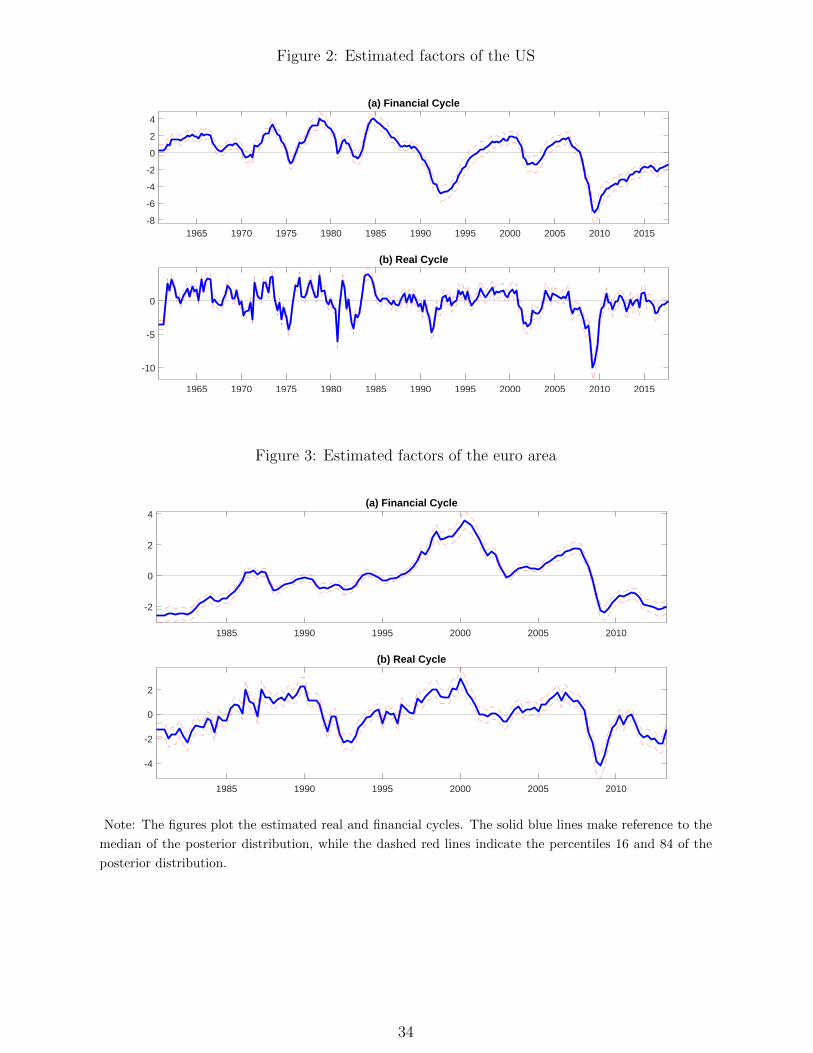
Figure 2: Estimated factors of the US

1965 1970 1975 1980 1985 1990 1995 2000 2005 2010 2015-8

-6

-4

-2

0

2

4

(a) Financial Cycle

1965 1970 1975 1980 1985 1990 1995 2000 2005 2010 2015

-10

-5

0

(b) Real Cycle

Figure 3: Estimated factors of the euro area

1985 1990 1995 2000 2005 2010

-2

0

2

4(a) Financial Cycle

1985 1990 1995 2000 2005 2010

-4

-2

0

2

(b) Real Cycle

Note: The figures plot the estimated real and financial cycles. The solid blue lines make reference to the

median of the posterior distribution, while the dashed red lines indicate the percentiles 16 and 84 of the

posterior distribution.

34

Figure 4: Business cycle with NBER recession dates for the US

Figure 5: Business cycle with CEPR recession dates for the euro area

Note: The figures show the business cycles in the US and euro area. The cycles have been extracted

using an HP filter with lambda = 1600 to extract the quarterly frequency. The recession dates are marked

in grey and come from the official sources: NBER for the US and CEPR for the euro area. To facilitate

comparison with the macroeconomic cycles estimated in our model, we use the same sample length.

35

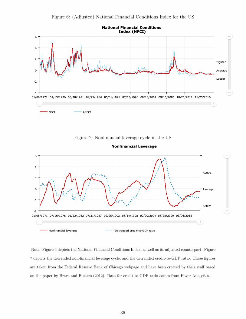
Figure 6: (Adjusted) National Financial Conditions Index for the US

Figure 7: Nonfinancial leverage cycle in the US

Note: Figure 6 depicts the National Financial Conditions Index, as well as its adjusted counterpart. Figure

7 depicts the detrended non-financial leverage cycle, and the detrended credit-to-GDP ratio. These figures

are taken from the Federal Reserve Bank of Chicago webpage and have been created by their staff based

on the paper by Brave and Butters (2012). Data for credit-to-GDP-ratio comes from Haver Analytics.

36

Figure 8: Estimated correlation between factors of the US

1970 1980 1990 2000 20100.2

0.3

0.4

0.5

0.6

0.7

0.8

Figure 9: Estimated correlation between factors of the euro area

1985 1990 1995 2000 2005 20100.3

0.4

0.5

0.6

0.7

0.8

0.9

Note: The figures plot the estimated time-varying correlation between the real and the financial cycle.

The solid blue line makes reference to the median of the posterior distribution, while the dashed red lines

indicate the percentiles 16 and 84 of the posterior distribution.

37

Figure 10: Impulse Responses Between Real and Financial Cycles for US

1

0

2 3 4

0.2

5 6 7 8

0.4

20109 10

Response of the Real Activity to a shock in Financial Conditions

11 200012

0.6

1314 1990151617 19801819 1970202122

1

0.1

2 3 4

0.2

5 6 7

0.3

8 20109 10

0.4

Response of the Financial Conditions to a shock in Real Activity

11 20001213

0.5

14 1990151617 19801819 1970202122

Note: The figure plots the estimated time-varying impulse responses for different horizons (h). The surface

makes reference to the median of the corresponding posterior distribution.

38

Figure 11: Impulse Responses Between Real and Financial Cycles for euro area

01 2

0.05

3 4 5

0.1

6 7 20108 9

0.15

10

Response of the Real Activity to a shock in Financial Conditions

20051112

0.2

2000131415 19951617 1990181920 19852122

0.05

1 2 3

0.1

4 5

0.15

6 7 20108

0.2

9 10

Response of the Financial Conditions to a shock in Real Activity

200511

0.25

12 20001314

0.3

15 19951617 1990181920 19852122

Note: The figure plots the estimated time-varying impulse responses for different horizons (h). The surface

makes reference to the median of the corresponding posterior distribution.

39

Figure 12: Financial (F) and real (R) factor loadings for the US

1970 1990 2010-0.5

0

0.5

1F1

1970 1990 2010-0.5

0

0.5

1F2

1970 1990 2010-0.5

0

0.5

1F3

1970 1990 2010-0.5

0

0.5

1F4

1970 1990 2010-0.5

0

0.5

1F5

1970 1990 2010-0.5

0

0.5

1F6

1970 1990 2010-0.5

0

0.5

1F7

1970 1990 2010-0.5

0

0.5

1F8

1970 1990 2010-0.5

0

0.5

1F9

1970 1990 2010-0.5

0

0.5

1F10

1970 1990 2010-0.5

0

0.5

1F11

1970 1990 2010-0.5

0

0.5

1F12

1970 1990 2010-0.5

0

0.5

1F13

1970 1990 2010-0.5

0

0.5

1F14

1970 1990 2010-0.5

0

0.5

1F15

1970 1990 2010-0.5

0

0.5

1F16

1970 1990 2010-0.5

0

0.5

1F17

1970 1990 2010-0.5

0

0.5

1F18

1970 1990 2010-0.5

0

0.5

1F19

1970 1990 2010-0.5

0

0.5

1F20

1970 1990 2010-0.5

0

0.5

1F21

1970 1990 2010-0.5

0

0.5

1F22

1970 1990 2010-0.5

0

0.5

1F23

1970 1990 2010-0.5

0

0.5

1R1

1970 1990 2010-0.5

0

0.5

1R2

1970 1990 2010-0.5

0

0.5

1R3

1970 1990 2010-0.5

0

0.5

1R4

1970 1990 2010-0.5

0

0.5

1R5

1970 1990 2010-0.5

0

0.5

1R6

1970 1990 2010-0.5

0

0.5

1R7

1970 1990 2010-0.5

0

0.5

1R8

1970 1990 2010-0.5

0

0.5

1R9

Note: These are the time-varying factor loadings in the financial cycle (above) and the real factor loadings

in the macroeconomic cycle (below). The solid blue lines make reference to the median of the posterior

distribution, while the dashed red lines indicate the percentiles 16 and 84 of the posterior distribution. For

the name of each of the loadings, we refer to Table 3.

40

Figure 13: Financial (F) and real (R) factor loadings for the euro area

1990 2000 2010-0.5

0

0.5

1F1

1990 2000 2010-0.5

0

0.5

1F2

1990 2000 2010-0.5

0

0.5

1F3

1990 2000 2010-0.5

0

0.5

1F4

1990 2000 2010-0.5

0

0.5

1F5

1990 2000 2010-0.5

0

0.5

1F6

1990 2000 2010-0.5

0

0.5

1F7

1990 2000 2010-0.5

0

0.5

1F8

1990 2000 2010-0.5

0

0.5

1F9

1990 2000 2010-0.5

0

0.5

1F10

1990 2000 2010-0.5

0

0.5

1F11

1990 2000 2010-0.5

0

0.5

1F12

1990 2000 2010-0.5

0

0.5

1F13

1990 2000 2010-0.5

0

0.5

1F14

1990 2000 2010-0.5

0

0.5

1F15

1990 2000 2010-0.5

0

0.5

1F16

1990 2000 2010-0.5

0

0.5

1F17

1990 2000 2010-0.5

0

0.5

1F18

1990 2000 2010-0.5

0

0.5

1F19

1990 2000 2010-0.5

0

0.5

1F20

1990 2000 2010-0.5

0

0.5

1F21

1990 2000 2010-0.5

0

0.5

1R1

1990 2000 2010-0.5

0

0.5

1R2

1990 2000 2010-0.5

0

0.5

1R3

1990 2000 2010-0.5

0

0.5

1R4

1990 2000 2010-0.5

0

0.5

1R5

1990 2000 2010-0.5

0

0.5

1R6

1990 2000 2010-0.5

0

0.5

1R7

1990 2000 2010-0.5

0

0.5

1R8

Note: These are the time-varying factor loadings in the financial cycle (above) and the real factor loadings

in the macroeconomic cycle (below). The solid blue lines make reference to the median of the posterior

distribution, while the dashed red lines indicate the percentiles 16 and 84 of the posterior distribution. For

the name of each of the loadings, we refer to Table 4.

41

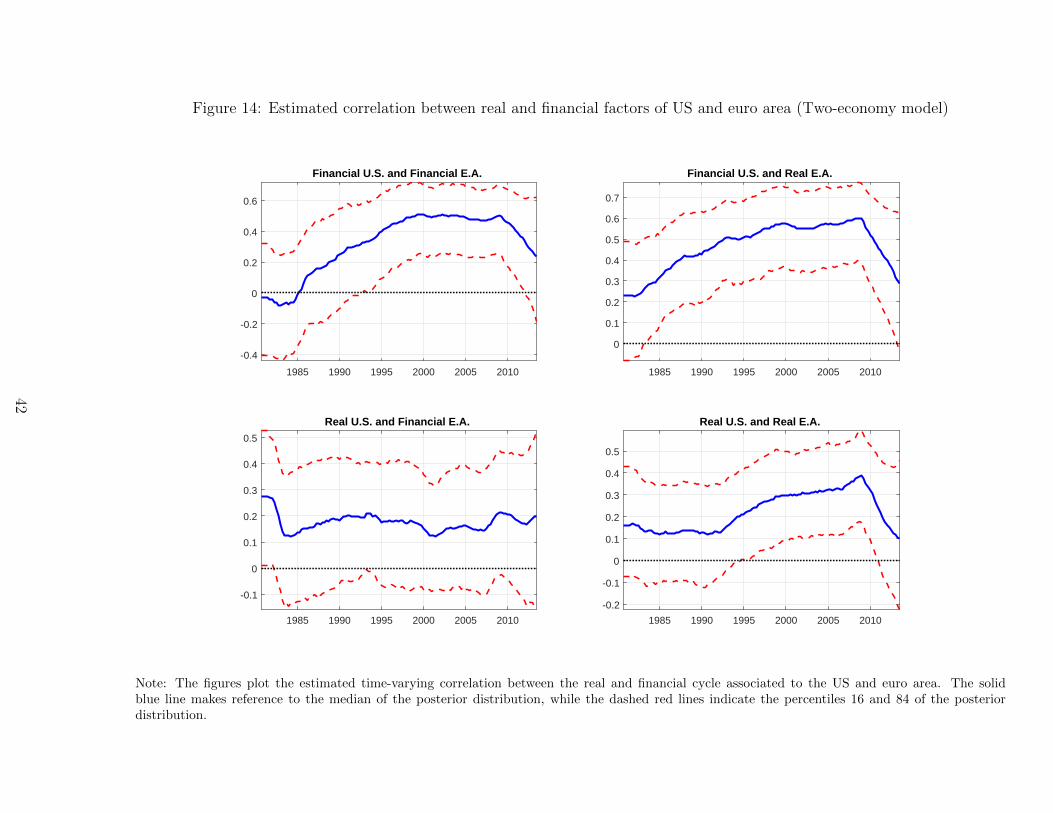
Figure 14: Estimated correlation between real and financial factors of US and euro area (Two-economy model)

1985 1990 1995 2000 2005 2010

-0.4

-0.2

0

0.2

0.4

0.6

Financial U.S. and Financial E.A.

1985 1990 1995 2000 2005 2010

0

0.1

0.2

0.3

0.4

0.5

0.6

0.7

Financial U.S. and Real E.A.

1985 1990 1995 2000 2005 2010

-0.1

0

0.1

0.2

0.3

0.4

0.5

Real U.S. and Financial E.A.

1985 1990 1995 2000 2005 2010

-0.2

-0.1

0

0.1

0.2

0.3

0.4

0.5

Real U.S. and Real E.A.

Note: The figures plot the estimated time-varying correlation between the real and financial cycle associated to the US and euro area. The solidblue line makes reference to the median of the posterior distribution, while the dashed red lines indicate the percentiles 16 and 84 of the posteriordistribution.

42

Figure 15: Macro-financial spillovers from the US to the euro area over time (Two-economy model)

0

1 2

0.1

3 4 5 6

0.2

7 8 20109

0.3

10

Response of the E.A. Real Activity to a shock in U.S. Real Activity

20051112

0.4

2000131415 19951617 1990181920 19852122

-0.11 2 3 4

0

5 6 7 8 20109

0.1

10

Response of the E.A. Real Activity to a shock in U.S. Financial Conditions

20051112 2000131415 19951617 1990181920 19852122

1

0.05

2 3 4 5

0.1

6 7 8 2010

0.15

9 10

Response of the E.A. Financial Conditions to a shock in U.S. Real Activity

200511

0.2

12 2000131415 19951617 1990181920 19852122

1 2 3

0.05

4 5 6 7 8 2010

0.1

9 10

Response of the E.A. Financial Conditions to a shock in U.S. Financial Conditions

20051112 200013

0.15

1415 19951617 1990181920 19852122

Note: The figure plots the estimated time-varying impulse responses for different horizons (h). The surface makes reference to the median of thecorresponding posterior distribution. The estimates are obtained by using sign and exclusion restrictions in the impact multiplier matrix to identifythe structural shocks.

43

Figure 16: Macro-financial spillovers from the euro area to the US over time (Two-economy model)

-0.05

1 2 3

0

4 5 6

0.05

7 8 20109

0.1

10

Response of the U.S. Real Activity to a shock in E.A. Real Activity

20051112

0.15

2000131415 19951617 1990181920 19852122

-0.05

1 2 3

0

4 5 6 7

0.05

8 20109 10

Response of the U.S. Real Activity to a shock in E.A. Financial Conditions

200511

0.1

12 2000131415 19951617 1990181920 19852122

1

-0.06

2 3 4 5

-0.04

6 7 8 2010

-0.02

9 10

Response of the U.S. Financial Conditions to a shock in E.A. Real Activity

20051112

0

2000131415 19951617 1990181920 19852122

-0.08

1 2 3

-0.06

4 5 6 7

-0.04

8 20109 10

Response of the U.S. Financial Conditions to a shock in E.A. Financial Conditions

2005

-0.02

1112 2000131415 19951617 1990181920 19852122

Note: The figure plots the estimated time-varying impulse responses for different horizons (h). The surface makes reference to the median of thecorresponding posterior distribution. The estimates are obtained by using sign and exclusion restrictions in the impact multiplier matrix to identifythe structural shocks.

44

A Online appendix

A.1 Implications for monetary and financial policy

In light of the tight interaction between the financial sector and the macroeconomy, the

feedback loops between the two and the intense cross-border spillovers from the US financial

sector to the euro area macroeconomy, the question is how should monetary and financial

policies adapt or evolve in order to tackle these challenges. Notably, financial policy has

gained a lot of importance since the Great Recession and has captured some of the territory

previously entrusted to monetary policy (financial stability). Moreover, it is not clear

whether the monetary and financial responses to shocks and frictions should be equivalent

in the US and in the euro area, given their asymmetric and distinct nature of spillovers.

While we are not attempting to provide a framework for (re)defining policy objectives,

targets and instruments, we wish to explore the implications of our findings for monetary

and macroprudential stance and provide some groundwork for further investigation.

The current high degree of synchronicity between macroeconomic and financial cycles

implies two things. First, disturbances in either sector will be transmitted almost com-

pletely to the other sector. Second, it is hard to disentangle the sphere of influence of

monetary and macroprudential policy, since their transmissions will be heavily aligned and

exert strong spillover effects/externality on the other. Moreover, taking into account that

the financial cycle is comparatively longer, it also means that the timing of their phases

might have important implications for both policies. While monetary policy impact on

shorter frequency, macroprudential policy does so on longer frequency. This means that,

it is possible for the economy to experience twin crises resulting in double-dip recessions

over a short period of time. Under this scenario, while the economy recovers from the first

recession, the financial cycle may start to contract, exerting downward pressures on the

macroeconomic cycle and resulting in another recession. And albeit both policies react op-

timally and according to their individual targets, the total impact might still be inadequate

and undesirable since the large overlapping set (or intersection) is overlooked.

Another equally important finding is the potential for financial shock spillover from the

US to the real and financial sectors of the euro area. Considering that the transmission

1

is mainly in one direction, the ECB should be very concerned about the developments

and fluctuations in the US financial sector. Bearing in mind that the transmission of US

financial shocks to euro area real activity is stronger than any other combination of cross-

border spillovers, this implies that the monetary policy should be concerned and respond

to US financial sector fluctuations to a higher extent than (traditional) financial policy.

The implications for monetary policy from these developments are of significant impor-

tance. First, monetary policy will and is forced to respond to developments in the financial

sector. Conversely, monetary policy must have a more prominent role to play in financial

sector activity compared to the pre-Great Recession optimum. Thus, despite all the effort

to insulate monetary policy from financial stability concerns and the realm of financial

policy, their influence is stronger than ever before in post-war history. Monetary policy

must devote much more efforts to understand, in real time, the particular point that the

financial cycle is on, and the potential risks to the monetary system and the macroeconomy.

This is particularly relevant to the ECB which must monitor, respond, and target both

internal and US financial disturbances. Financial policy, on the other hand, must price in

the reaction and targets of monetary policy. There are two ways of achieving this. Either

a leader-follower arrangement where monetary policy is the leader, and financial policy

the follower. Alternatively, a close interaction between the policies will be necessary at all

points in the business cycle, perhaps even explicitly. Also, the monetary stance needs to

adjust and incorporate a much broader and deeper map of financial exposures and risks

into its map. Lastly, it may well be necessary to expand the monetary policy toolkit to

include multiple instruments and (clearly defined) targets. In this new environment, it is

hard to conceive how price stability will achieve the broader objective of macroeconomic

growth and stability. Only in cooperation with other instruments, possibly those employed

during the unconventional monetary policy phase, will that objective be achieved.

A.2 Estimation algorithm

The proposed algorithm relies on Bayesian methods and uses the Gibss sampler to

simulate the posterior distribution of parameters and latent variables involved in the time-

varying parameter factor model. Define the following vectors containing information on the

2

nfand nrfinancial and real activity variables, respectively, YT = F1f ,t, ..., Fnf ,t, R1r,t, ..., Rnr,tTt=1,

real activity index, fT = ftTt=1, financial conditions index, rT = rtTt=1, factor loadings,

Λx,T = Λx,tTt=1, where Λx,t = (λ1x,t, ..., λnx,t)′, for x = f, r, and autoregressive coeffi-

cients, ΦT = vec(Φ1,t), ..., vec(Φk,t)Tt=1. The algorithm consists of the following steps:

• Step 1 : Sample fT , and rT from P (fT , rT |Λx,T , ΦT ,Σ,Ω,Ψω,Ψw, YT )

The model in equations (1)-(2), with k = 2, can be cast in a state-space representation

with measurement equation given by,

F1f ,t

...

Fnf ,t

R1r,t

...

Rnr,t

=

λ1f ,t 0 0 0...

......

...

λnf ,t 0 0 0

0 λ1r,t 0 0...

......

...

0 λnr,t 0 0

ft

rt

ft−1

rt−1

+

v1f ,t...

vnf ,t

v1r,t...

vnr,t

, (7)

and transition equation defined as,ft

rt

ft−1

rt−1

=

φ(1)ff,t φ

(1)fr,t φ

(2)ff,t φ

(2)fr,t

φ(1)rf,t φ

(1)rr,t φ

(2)rf,t φ

(2)rr,t

1 0 0 0

0 1 0 0

ft−1

rt−1

ft−2

rt−2

+

uf,t

ur,t

0

0

. (8)

Conditional on Λx,T and ΦT , equations (7)-(8) constitute a linear and Gaussian state-space

model, and the Carter and Kohn simulation smoother is applied to generate inferences of

the factors.

• Step 2 : Sample Ψw from P (Ψw|ΦT , YT )

To sample the variance of the time-varying autoregressive coefficient innovations, we use

an inverse Wishart prior distribution, IW (η, v), with η = τ and v = κ2 × τ × ΨOLSw ,

where τ = 80 is the size of the training sample, ΨOLSw is the variance of the autoregressive

coefficient matrix estimated by OLS based on the training sample, and κ = 0.2 is a scaling

3

factor. Hence, draws of Ψw are generated from the posterior distribution,

Ψw ∼ IW (η, v),

where

η = η + T

v = v + (φt − φt−1)′(φt − φt−1).

• Step 3 : Sample ΦT from P (ΦT |fT , rT ,Ψw,Σ, YT )

Conditional on the factors, the time-varying coefficient VAR model that drives the dynamics

of the factors can be compactly expressed in the following state-space form,

yt = X ′tφt + vt, vt ∼ N(0,Σ)

φt = φt−1 +wt, wt ∼ N(0,Ψw)

where yt = (ft, rt)′, X t = Im ⊗ [1,y′t−1, ...,y

′t−k] are observed, with m = 2 being the

number of factors, and φt is the latent vector. Therefore, as in Step 1, the Carter and

Kohn algorithm is applied to generate draws of ΦT . To achieve stability in the system, this

step is repeated until it generates a draw of φt that fulfills the stationarity conditions for

all time periods in the sample.

• Step 4 : Sample Σ from P (Σ|fT , rT , ΦT ,Ψw, YT )

To sample the variance of reduced form innovations, we use an inverse Wishart prior dis-

tribution, IW (m, ν), with m = m + 1 and ν = Im. Hence, draws of Σ are generated from

the posterior distribution,

Σ ∼ IW (m, ν),

where

m = m+ T

ν = ν + (yt −X ′tφt)′(yt −X ′tφt).

4

• Step 5 : Sample Λx,T from P (Λx,T |fT , rT ,Ω,Ψω, YT )

Given that Ω is assumed to be a diagonal matrix, each time-varying loading can be sampled

independently. Accordingly, we use the following state-space representation,

Xix,t = λix,txt + vix,t, vix,t ∼ N(0,Ω[ix,ix])

λix,t = λix,t−1 + ωix,t, ωix,t ∼ N(0,Ψω,[ix,ix])

for observed variables X = F,R, latent factors x = f, r, and i = 1, ..., n. Next, the Carter

and Kohn algorithm is applied to generate draws of the elements in Λx,T .

• Step 6 : Sample Ψω from P (Ψω|Λx,T , YT )

To sample, independently, the variance of the time-varying loading innovations, we use an

inverse Gamma prior distribution, IG(u, z), with u = 0.1× T and z = 0.12. Hence, draws

of Ψw are generated from the posterior distribution,

Ψw ∼ IG(u, z),

where

u = u+ T

z = z + (λix,t − λix,t−1)′(λix,t − λix,t−1).

• Step 7 : Sample Ω from P (Ω|fT , rT , Λx,T , YT )

To sample, independently, the variance of the idiosyncratic terms, we use an inverse Gamma

prior distribution, IG(l, o), with l = 0 and o = 0. Accordingly, draws of the entries in the

diagonal of Ω are generated from the posterior distribution,

Ωix ∼ IG(l, o),

5

for i = 1, ..., n, X = F,R, and x = f, r, where

l = l + T

o = o+ (Xix,t − λix,txt)′(Xix,t − λix,txt).

To approximate the posterior distribution of both the parameters and latent variables

involved in the model, each step of the algorithm is recursively repeated M = 22, 000 times,

discarding the first m = 20, 000 iterations to ensure convergence.

6

A.3 Alternative Identification Schemes

Table 5: Recursive Identification for the Two-economy model

Fin. Shock E.A. Real Shock E.A. Fin. Shock US Real Shock US

Financial Cycle E.A. ∗ ∗ ∗ ∗Real Cycle E.A. 0 ∗ ∗ ∗Financial Cycle US 0 0 ∗ ∗Real Cycle US 0 0 0 ∗Note: The symbol ∗ indicates that no restriction is imposed in the corresponding relationship.

Table 6: Alternative Sign and Exclusion Restrictions for the Two-economy model

Fin. Shock E.A. Real Shock E.A. Fin. Shock US Real Shock US

Financial Cycle E.A. + + ∗ ∗Real Cycle E.A. 0 + ∗ ∗Financial Cycle US 0 0 + +Real Cycle US 0 0 0 +

Note: The symbol ∗ indicates that no restriction is imposed in the corresponding relationship.

7

A.4 Additional Figures

Figure 17: Estimated factors of the US - Principal Component

1965 1970 1975 1980 1985 1990 1995 2000 2005 2010 2015

-5

0

5

-1.5

-1

-0.5

0

0.5

1

(a) Financial Cycle

1965 1970 1975 1980 1985 1990 1995 2000 2005 2010 2015

-10

-5

0

5

-2

-1

0

1

(b) Real Cycle

Figure 18: Estimated factors of the euro area - Principal Component

1985 1990 1995 2000 2005 2010

-2

0

2

4

-1

-0.5

0

0.5

1

1.5(a) Financial Cycle

1985 1990 1995 2000 2005 2010-6

-4

-2

0

2

4

-1.5

-1

-0.5

0

0.5

1

(b) Real Cycle

Note: The figures plot the estimated real and financial cycles. The solid blue lines make reference to

the median of the posterior distribution, while the dashed red lines indicate the percentiles 5 and 95 of

the posterior distribution, and the solid green line plots the corresponding factor estimated with principal

components, and aligned with the right axis.

8

Figure 19: Estimated correlation between factors of the US - Orthogonal Innovations

1970 1980 1990 2000 2010-0.2

0

0.2

0.4

0.6

0.8

1

Figure 20: Estimated correlation between factors of the euro area - Orthogonal Innovations

1985 1990 1995 2000 2005 2010-0.1

0

0.1

0.2

0.3

0.4

0.5

0.6

0.7

0.8

0.9

Note: The figures plot the estimated time-varying correlation between the real and financial cycle. The

solid blue line makes reference to the median of the posterior distribution, while the dashed red lines

indicate the percentiles 16 and 84 of the posterior distribution. The estimates are obtained by assuming

orthogonality in the innovations of the factors.

9

Figure 21: Estimated correlation between factors of the US - Break in Volatility

1970 1980 1990 2000 20100.2

0.3

0.4

0.5

0.6

0.7

0.8

Note: The figure plots the estimated time-varying correlation between the real and financial cycles. The

solid blue line makes reference to the median of the posterior distribution, while the dashed red lines

indicate the percentiles 16 and 84 of the posterior distribution. The estimates are obtained by assuming a

break in the volatility of the factors occurred in 1985.

10

Figure 22: Cumulated Impulse Response Patterns for US

(a) Response of financial conditions to a financial shock

1970 1990 20100

0.5

1

1.5h=1

1970 1990 20100

2

4

6h=10

1970 1990 20100

2

4

6

8

10h=20

(b) Response of real activity to a financial shock

1970 1990 20100

0.5

1

1.5h=1

1970 1990 2010-2

0

2

4h=10

1970 1990 2010-2

0

2

4

6h=20

(c) Response of financial conditions to a real shock

1970 1990 20100

0.5

1

1.5h=1

1970 1990 20100

2

4

6

8h=10

1970 1990 20100

5

10

15h=20

(d) Response of real activity to a real shock

1970 1990 20100

1

2

3

4h=1

1970 1990 20100

2

4

6

8

10h=10

1970 1990 20100

2

4

6

8

10h=20

Note: The figure plots the estimated time-varying cumulated impulse responses for different horizons (h).

The solid blue lines make reference to the median of the posterior distribution, while the dashed red lines

indicate the percentiles 16 and 84 of the posterior distribution.

11

Figure 23: Cumulated Impulse Response Patterns for euro area

(a) Response of financial conditions to a financial shock

1990 2000 20100

0.2

0.4

0.6

0.8h=1

1990 2000 20100

1

2

3

4h=10

1990 2000 20100

2

4

6h=20

(b) Response of real activity to a financial shock

1990 2000 20100

0.1

0.2

0.3

0.4h=1

1990 2000 2010-0.5

0

0.5

1

1.5

2h=10

1990 2000 2010-1

0

1

2

3

4h=20

(c) Response of financial conditions to a real shock

1990 2000 20100

0.2

0.4

0.6h=1

1990 2000 20100

1

2

3

4h=10

1990 2000 20100

2

4

6

8h=20

(d) Response of real activity to a real shock

1990 2000 20100

0.5

1

1.5

2h=1

1990 2000 20100

2

4

6h=10

1990 2000 20100

2

4

6

8h=20

Note: The figure plots the estimated time-varying cumulated impulse responses for different horizons (h).

The solid blue lines make reference to the median of the posterior distribution, while the dashed red lines

indicate the percentiles 16 and 84 of the posterior distribution.

12

Figure 24: Impulse Responses Between Real and Financial Cycles for US - OrthogonalInnovations

0

1 2

0.2

3 4

0.4

5 6

0.6

7 8 2010

0.8

9 10

Response of the Real Activity to a shock in Financial Conditions

1

11 200012

1.2

1314 1990151617 19801819 1970202122

-0.02

1 2

0

3 4 5

0.02

6 7 8

0.04

20109 10

Response of the Financial Conditions to a shock in Real Activity

0.06

11 20001213

0.08

14 1990151617 19801819 1970202122

Note: The figure plots the estimated time-varying impulse responses for different horizons (h). The surface

makes reference to the median of the corresponding posterior distribution. The estimates are obtained by

assuming orthogonality in the innovations of the factors.

13

Figure 25: Impulse Responses Between Real and Financial Cycles for euro area - OrthogonalInnovations

01 2 3

0.1

4 5 6 7

0.2

20108 9 10

Response of the Real Activity to a shock in Financial Conditions

200511

0.3

12 2000131415 19951617 1990181920 19852122

01 2 3

0.05

4 5 6 7

0.1

20108 9 10

Response of the Financial Conditions to a shock in Real Activity

200511

0.15

12 2000131415 19951617 1990181920 19852122

Note: The figure plots the estimated time-varying impulse responses for different horizons (h). The surface

makes reference to the median of the corresponding posterior distribution. The estimates are obtained by

assuming orthogonality in the innovations of the factors.

14

Figure 26: Impulse Responses Between Real and Financial Cycles for US - Break in Volatil-ity

-0.21

0

2 3 4

0.2

5 6

0.4

7 8 20109

0.6

10

Response of the Real Activity to a shock in Financial Conditions

11 2000

0.8

121314

1

1990151617 19801819 1970202122

1 2 3 4

0.1

5 6 7

0.2

1970 8

Response of the Financial Conditions to a shock in Real Activity

9

0.3

101980 11

0.4

12131990

0.5

141516

0.6

2000 1718192010 202122

Note: The figure plots the estimated time-varying impulse responses for different horizons (h). The surface

makes reference to the median of the corresponding posterior distribution. The estimates are obtained by

assuming a break in the volatility of the factors occurred in 1985.

15

Figure 27: Forecast Error Variance Decomposition for US

(a) Contribution of financial shocks to financial conditions

1970 1990 20100

0.2

0.4

0.6

0.8

1h=1

1970 1990 20100

0.2

0.4

0.6

0.8

1h=10

1970 1990 20100

0.2

0.4

0.6

0.8

1h=20

(b) Contribution of financial shocks to real activity

1970 1990 20100

0.2

0.4

0.6

0.8

1h=1

1970 1990 20100

0.2

0.4

0.6

0.8

1h=10

1970 1990 20100

0.2

0.4

0.6

0.8

1h=20

(c) Contribution of real shocks to financial conditions

1970 1990 20100

0.2

0.4

0.6

0.8

1h=1

1970 1990 20100

0.2

0.4

0.6

0.8

1h=10

1970 1990 20100

0.2

0.4

0.6

0.8

1h=20

(d) Contribution of real shocks to real activity

1970 1990 20100

0.2

0.4

0.6

0.8

1h=1

1970 1990 20100

0.2

0.4

0.6

0.8

1h=10

1970 1990 20100

0.2

0.4

0.6

0.8

1h=20

Note: The figure plots the estimated time-varying forecast error variance decomposition for different

horizons (h). The solid blue lines make reference to the median of the posterior distribution, while the

dashed red lines indicate the percentiles 16 and 84 of the posterior distribution.

16

Figure 28: Forecast Error Variance Decomposition for euro area

(a) Contribution of financial shocks to financial conditions

1990 2000 20100

0.2

0.4

0.6

0.8

1h=1

1990 2000 20100

0.2

0.4

0.6

0.8

1h=10

1990 2000 20100

0.2

0.4

0.6

0.8

1h=20

(b) Contribution of financial shocks to real activity

1990 2000 20100

0.2

0.4

0.6

0.8

1h=1

1990 2000 20100

0.2

0.4

0.6

0.8

1h=10

1990 2000 20100

0.2

0.4

0.6

0.8

1h=20

(c) Contribution of real shocks to financial conditions

1990 2000 20100

0.2

0.4

0.6

0.8

1h=1

1990 2000 20100

0.2

0.4

0.6

0.8

1h=10

1990 2000 20100

0.2

0.4

0.6

0.8

1h=20

(d) Contribution real shocks to real activity

1990 2000 20100

0.2

0.4

0.6

0.8

1h=1

1990 2000 20100

0.2

0.4

0.6

0.8

1h=10

1990 2000 20100

0.2

0.4

0.6

0.8

1h=20

Note: The figure plots the estimated time-varying forecast error variance decomposition for different

horizons (h). The solid blue lines make reference to the median of the posterior distribution, while the

dashed red lines indicate the percentiles 16 and 84 of the posterior distribution.

17

Figure 29: Estimated factors of the US and euro area (Two-economy model)

1985 1990 1995 2000 2005 2010

-2

0

2

4(a) Euro Area Financial Cycle

1985 1990 1995 2000 2005 2010

-6

-4

-2

0

2

4

(b) Euro Area Real Cycle

1985 1990 1995 2000 2005 2010

-4

-3

-2

-1

0

1

2

(c) U.S. Financial Cycle

1985 1990 1995 2000 2005 2010

-6

-4

-2

0

2

(d) U.S. Real Cycle

Note: The figures plot the estimated real and financial cycles for the US and euro area obtained with the (joint) two-economy model. The solidblue lines make reference to the median of the posterior distribution, while the dashed red lines indicate the percentiles 16 and 84 of the posteriordistribution.

18

Figure 30: Estimated correlation between factors associated to a given economy (Two-economy model)

1985 1990 1995 2000 2005 2010

0.1

0.2

0.3

0.4

0.5

0.6

0.7

(a) Real and Financial of U.S.

1985 1990 1995 2000 2005 2010

0.2

0.3

0.4

0.5

0.6

0.7

0.8

(b) Real and Financial of E.A.

Note: The figure plots the estimated time-varying correlation between the business and financial cycles as-

sociated to a given economy. The solid blue line makes reference to the median of the posterior distribution,

while the dashed red lines indicate the percentiles 16 and 84 of the posterior distribution.

19

Figure 31: Cumulated Impulse Response Patterns: Effect of US on E.A.

(a) Response of the E.A. Real Activity to a shock in US Real Activity

1990 2000 20100

0.5

1

1.5h=1

1990 2000 20100

1

2

3

4

5h=10

1990 2000 20100

2

4

6h=20

(b) Response of the E.A. Real Activity to a shock in US FinancialConditions

1990 2000 2010-0.4

-0.2

0

0.2

0.4h=1

1990 2000 2010-1

0

1

2

3h=10

1990 2000 2010-2

0

2

4

6h=20

(c) Response of the E.A. Financial Conditions to a shock in US RealActivity

1990 2000 20100

0.2

0.4

0.6h=1

1990 2000 20100

1

2

3

4h=10

1990 2000 2010-2

0

2

4

6

8h=20

(d) Response of the E.A. Financial Conditions to a shock in USFinancial Conditions

1990 2000 2010-0.4

-0.2

0

0.2

0.4h=1

1990 2000 2010-2

-1

0

1

2

3h=10

1990 2000 2010-2

0

2

4

6h=20

Note: The figure plots the estimated time-varying cumulated impulse responses for different horizons (h).

The solid blue lines make reference to the median of the posterior distribution, while the dashed red lines

indicate the percentiles 16 and 84 of the posterior distribution.

20

Figure 32: Cumulated Impulse Response Patterns: Effect of E.A. on US

(a) Response of the US Real Activity to a shock in E.A. Real Activity

1990 2000 2010-0.1

0

0.1

0.2

0.3

0.4h=1

1990 2000 2010-2

-1

0

1

2h=10

1990 2000 2010-2

-1

0

1

2h=20

(b) Response of the US Real Activity to a shock in E.A. FinancialConditions

1990 2000 2010-0.2

0

0.2

0.4

0.6h=1

1990 2000 2010-2

-1

0

1

2h=10

1990 2000 2010-2

-1

0

1

2h=20

(c) Response of the US Financial Conditions to a shock in E.A. RealActivity

1990 2000 2010-0.1

-0.05

0

0.05

0.1h=1

1990 2000 2010-1.5

-1

-0.5

0

0.5

1h=10

1990 2000 2010-3

-2

-1

0

1h=20

(d) Response of the US Financial Conditions to a shock in E.A.Financial Conditions

1990 2000 2010-1

-0.5

0

0.5

1h=1

1990 2000 2010-3

-2

-1

0

1

2h=10

1990 2000 2010-4

-2

0

2h=20

Note: The figure plots the estimated time-varying cumulated impulse responses for different horizons (h).

The solid blue lines make reference to the median of the posterior distribution, while the dashed red lines

indicate the percentiles 16 and 84 of the posterior distribution.

21

Figure 33: Macro-financial spillovers from the US to the euro area over time - Cholesky

-0.1

1 2 3

0

4 5 6 7

0.1

8 20109 10

Response of the E.A. Real Activity to a shock in U.S. Real Activity

200511

0.2

12 2000131415 19951617 1990181920 19852122

0

1 2 3 4

0.1

5 6 7 8 20109

0.2

10

Response of the E.A. Real Activity to a shock in U.S. Financial Conditions

20051112 2000131415 19951617 1990181920 19852122

1

0.05

2 3 4 5

0.1

6 7 8 2010

0.15

9 10

Response of the E.A. Financial Conditions to a shock in U.S. Real Activity

20051112

0.2

2000131415 19951617 1990181920 19852122

1 2

0.05

3 4 5 6

0.1

7 8 20109 10

0.15

Response of the E.A. Financial Conditions to a shock in U.S. Financial Conditions

20051112 200013

0.2

1415 19951617 1990181920 19852122

Note: The figure plots the estimated time-varying impulse responses for different horizons (h). The surface makes reference to the median of thecorresponding posterior distribution. The estimates are obtained by using Cholesky factorization to identify the structural shocks.

22

Figure 34: Macro-financial spillovers from the euro area to the US over time - Cholesky

1 2

0

3 4 5 6

0.1

7 8 20109 10

Response of the U.S. Real Activity to a shock in E.A. Real Activity

200511

0.2

12 2000131415 19951617 1990181920 19852122

1 2

-0.05

3 4 5 6

0

7 8 20109 10

Response of the U.S. Real Activity to a shock in E.A. Financial Conditions

0.05

20051112 2000131415 19951617 1990181920 19852122

-0.11 2 3 4

-0.05

5 6 7 8 20109

0

10

Response of the U.S. Financial Conditions to a shock in E.A. Real Activity

20051112 2000131415 19951617 1990181920 19852122

1 2

-0.06

3 4 5 6

-0.04

7 8 20109 10

-0.02

Response of the U.S. Financial Conditions to a shock in E.A. Financial Conditions

20051112 20001314

0

15 19951617 1990181920 19852122

Note: The figure plots the estimated time-varying impulse responses for different horizons (h). The surface makes reference to the median of thecorresponding posterior distribution. The estimates are obtained by using Cholesky factorization to identify the structural shocks.

23

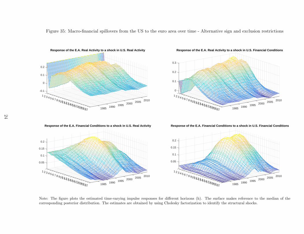
Figure 35: Macro-financial spillovers from the US to the euro area over time - Alternative sign and exclusion restrictions

-0.1

1 2 3

0

4 5 6 7 8

0.1

20109 10

Response of the E.A. Real Activity to a shock in U.S. Real Activity

20051112

0.2

2000131415 19951617 1990181920 19852122

0

1 2 3 4

0.1

5 6 7 8 20109

0.2

10

Response of the E.A. Real Activity to a shock in U.S. Financial Conditions

20051112 20001314

0.3

15 19951617 1990181920 19852122

1 2

0.05

3 4 5

0.1

6 7 8 20109

0.15

10

Response of the E.A. Financial Conditions to a shock in U.S. Real Activity

20051112

0.2

2000131415 19951617 1990181920 19852122

1 2

0.05

3 4 5 6

0.1

7 8 20109

0.15

10

Response of the E.A. Financial Conditions to a shock in U.S. Financial Conditions

20051112 200013

0.2

1415 19951617 1990181920 19852122

Note: The figure plots the estimated time-varying impulse responses for different horizons (h). The surface makes reference to the median of thecorresponding posterior distribution. The estimates are obtained by using Cholesky factorization to identify the structural shocks.

24

Figure 36: Macro-financial spillovers from the euro area to the US over time - Alternative sign and exclusion restrictions

1 2

0

3 4 5 6

0.1

7 8 20109 10

Response of the U.S. Real Activity to a shock in E.A. Real Activity

200511

0.2

12 2000131415 19951617 1990181920 19852122

1

-0.05

2 3 4 5 6

0

7 8 20109 10

0.05

Response of the U.S. Real Activity to a shock in E.A. Financial Conditions

20051112 20001314

0.1

15 19951617 1990181920 19852122

-0.11 2 3 4

-0.05

5 6 7 8 20109

0

10

Response of the U.S. Financial Conditions to a shock in E.A. Real Activity

20051112 20001314

0.05

15 19951617 1990181920 19852122

-0.081 2 3

-0.06

4 5 6

-0.04

7 8 20109 10

Response of the U.S. Financial Conditions to a shock in E.A. Financial Conditions

2005

-0.02

1112 20001314

0

15 19951617 1990181920 19852122

Note: The figure plots the estimated time-varying impulse responses for different horizons (h). The surface makes reference to the median of thecorresponding posterior distribution. The estimates are obtained by using Cholesky factorization to identify the structural shocks.

25

W O R K I N G P A P E R — D A N M AR K S N A T IO N A L B A N K

1 0 M AR C H 2 0 2 0 — N O . 15 3

As a rule, Working Papers are not translated, but are available in the original language used by the contributor.

Danmarks Nationalbank's Working Paper are published in PDF format at www.nationalbanken.dk. A free electronic subscription is also available at the website. The subscriber receives an e-mail notification whenever a new Working Paper is published.

Text may be copied from this publication provided that the source is specifically stated. Changes to or misrepresentation of the content are not permitted.

Please direct any enquiries directly to the contributors or to Danmarks Nationalbank, Communications, Kommunikation@nationalbanken.dk.