macroeconomic theory i - rutgers...
TRANSCRIPT

Macroeconomic Theory I
Cesar E. TamayoDepartment of Economics, Rutgers University
Class Notes: Fall 2010

Contents
I Deterministic models 4
1 The Solow Model 51.1 Dynamics . . . . . . . . . . . . . . . . . . . . . . . . . . . . . . . . . . . . . . . . 61.2 Balanced growth . . . . . . . . . . . . . . . . . . . . . . . . . . . . . . . . . . . . 61.3 The golden rule . . . . . . . . . . . . . . . . . . . . . . . . . . . . . . . . . . . . . 61.4 Quantitative implications . . . . . . . . . . . . . . . . . . . . . . . . . . . . . . . 71.5 Solow growth accounting . . . . . . . . . . . . . . . . . . . . . . . . . . . . . . . . 8
2 Optimal growth 92.1 Optimal growth in discrete time . . . . . . . . . . . . . . . . . . . . . . . . . . . 92.2 Assumptions . . . . . . . . . . . . . . . . . . . . . . . . . . . . . . . . . . . . . . 92.3 The sequential method: Lagrange . . . . . . . . . . . . . . . . . . . . . . . . . . . 102.4 The recursive method: dynamic programming . . . . . . . . . . . . . . . . . . . . 10
2.4.1 The Envelope Theorem approach . . . . . . . . . . . . . . . . . . . . . . . 132.5 Balanced growth and steady state . . . . . . . . . . . . . . . . . . . . . . . . . . 142.6 Linearization . . . . . . . . . . . . . . . . . . . . . . . . . . . . . . . . . . . . . . 152.7 Equilibrium growth and welfare theorems . . . . . . . . . . . . . . . . . . . . . . 162.8 Extensions to the optimal growth model . . . . . . . . . . . . . . . . . . . . . . . 18
2.8.1 Assets in the OGM . . . . . . . . . . . . . . . . . . . . . . . . . . . . . . . 182.8.2 The role of government in OGM . . . . . . . . . . . . . . . . . . . . . . . 19
2.9 Optimal Growth in continuous time . . . . . . . . . . . . . . . . . . . . . . . . . 212.9.1 Steady State . . . . . . . . . . . . . . . . . . . . . . . . . . . . . . . . . . 222.9.2 Tobin�s q . . . . . . . . . . . . . . . . . . . . . . . . . . . . . . . . . . . . 23
3 Overlapping generations (OLG) 253.1 OLG in economies with production (Diamond�s) . . . . . . . . . . . . . . . . . . 25
3.1.1 Log-utility and Cobb-Douglas technology . . . . . . . . . . . . . . . . . . 273.1.2 Steady state . . . . . . . . . . . . . . . . . . . . . . . . . . . . . . . . . . . 283.1.3 Golden rule and dynamic ine¢ ciency . . . . . . . . . . . . . . . . . . . . . 293.1.4 The role of Government. . . . . . . . . . . . . . . . . . . . . . . . . . . . . 293.1.5 Social security . . . . . . . . . . . . . . . . . . . . . . . . . . . . . . . . . 303.1.6 Restoring Ricardian equivalence . . . . . . . . . . . . . . . . . . . . . . . 31
3.2 OLG in pure exchange economies (Samuelson�s) . . . . . . . . . . . . . . . . . . . 323.2.1 Homogeneity within generation . . . . . . . . . . . . . . . . . . . . . . . . 323.2.2 The role of money . . . . . . . . . . . . . . . . . . . . . . . . . . . . . . . 343.2.3 Fiscal policy and the La¤er curve . . . . . . . . . . . . . . . . . . . . . . . 363.2.4 Monetary equilibria with money growth . . . . . . . . . . . . . . . . . . . 373.2.5 Within generation heterogeneity . . . . . . . . . . . . . . . . . . . . . . . 373.2.6 The real bills doctrine . . . . . . . . . . . . . . . . . . . . . . . . . . . . . 39
1
II Stochastic models 41
4 Stochastic Optimal growth 424.1 Uncertainty in the neoclassical OGM . . . . . . . . . . . . . . . . . . . . . . . . . 42
4.1.1 Non-stochastic steady state . . . . . . . . . . . . . . . . . . . . . . . . . . 434.1.2 Stationary distribution . . . . . . . . . . . . . . . . . . . . . . . . . . . . . 434.1.3 Log-linear approximation . . . . . . . . . . . . . . . . . . . . . . . . . . . 44
4.2 Solution method 1: Blanchard-Khan . . . . . . . . . . . . . . . . . . . . . . . . . 444.3 Impulse response functions (IRF) . . . . . . . . . . . . . . . . . . . . . . . . . . . 45
5 RBC models 465.1 The baseline RBC model . . . . . . . . . . . . . . . . . . . . . . . . . . . . . . . . 46
5.1.1 The general case . . . . . . . . . . . . . . . . . . . . . . . . . . . . . . . . 465.1.2 CRRA utility and Cobb-Douglas production . . . . . . . . . . . . . . . . 475.1.3 The log-linear system . . . . . . . . . . . . . . . . . . . . . . . . . . . . . 47
5.2 Labor productivity (King, Plosser & Rebelo, 1988) . . . . . . . . . . . . . . . . . 485.3 Solution method 2: Sim�s GENSYS . . . . . . . . . . . . . . . . . . . . . . . . . . 505.4 Varieties of RBC models . . . . . . . . . . . . . . . . . . . . . . . . . . . . . . . . 51
5.4.1 Asset pricing models (Lucas, Shiller) . . . . . . . . . . . . . . . . . . . . . 515.5 Calibration . . . . . . . . . . . . . . . . . . . . . . . . . . . . . . . . . . . . . . . 525.6 Estimation methods . . . . . . . . . . . . . . . . . . . . . . . . . . . . . . . . . . 52
5.6.1 Generalized method of moments (GMM) . . . . . . . . . . . . . . . . . . . 52
III Appendixes 56
A The dynamic programming method 57A.1 Guess and verify . . . . . . . . . . . . . . . . . . . . . . . . . . . . . . . . . . . . 58A.2 Value function iteration . . . . . . . . . . . . . . . . . . . . . . . . . . . . . . . . 59A.3 Solving for the policy functions . . . . . . . . . . . . . . . . . . . . . . . . . . . . 60A.4 Properties of the BFE . . . . . . . . . . . . . . . . . . . . . . . . . . . . . . . . . 61A.5 The Envelope Theorem: an application . . . . . . . . . . . . . . . . . . . . . . . . 62
B The Maximum Principle 66B.1 Discrete time . . . . . . . . . . . . . . . . . . . . . . . . . . . . . . . . . . . . . . 66B.2 Continuous time . . . . . . . . . . . . . . . . . . . . . . . . . . . . . . . . . . . . 68
B.2.1 Current value vs. present value Hamiltonian . . . . . . . . . . . . . . . . 68
C First-Order Di¤erence Equations and AR(1) 70C.1 The AR(1) process . . . . . . . . . . . . . . . . . . . . . . . . . . . . . . . . . . . 70
C.1.1 Representation and properties . . . . . . . . . . . . . . . . . . . . . . . . . 70C.1.2 Conditional Distribution . . . . . . . . . . . . . . . . . . . . . . . . . . . . 71C.1.3 Unconditional Distribution . . . . . . . . . . . . . . . . . . . . . . . . . . 71
C.2 Linear First-Order Di¤erence Equations (FODE) . . . . . . . . . . . . . . . . . . 72C.2.1 Induction & Geometric Series . . . . . . . . . . . . . . . . . . . . . . . . . 72C.2.2 Homogeneous part and General solution . . . . . . . . . . . . . . . . . . . 73C.2.3 Asymptotic Stability . . . . . . . . . . . . . . . . . . . . . . . . . . . . . . 74
C.3 Systems of linear FODE (or VDE) . . . . . . . . . . . . . . . . . . . . . . . . . . 75C.3.1 Asymptotic stability . . . . . . . . . . . . . . . . . . . . . . . . . . . . . . 76
2

Summary
These notes summarize the material of a �rst semester graduate course in Macroeconomictheory. The �rst sections focus on deterministic growth models and models of overlappinggenerations (OLG). Later sections are dedicated to stochastic models, including neoclassicalgrowth and real business cycles models. The appendixes cover some mathematical materialrequired for solving simple macro models. The notes are freely based on: Acemoglu (2008),Romer (2001), Stokey and Lucas (1989), Ljungqvist and Sargent (2004), Dave and De Jong(2011), Dixit (1990), Levy (1992) and lecture notes from Professor Roberto Chang from RutgersUniversity. Naturally, all errors and omissions are my own.A word on notation: Throughout these notes, x� will be used to denote a speci�c solution
(optima), �x will be used for steady states in di¤erence (di¤erential) equations and x will beused for ln (x=�x). When applicable, upper cases will stand for economy-wide values of variables,while lower cases will stand for per-capita (per-e¤ective labor) variables. Finally, in stochasticmodels E0 or simply E will denote unconditional expectations while Et will stand for expectationsconditional on information available at t:
3

Part I
Deterministic models
4

Chapter 1
The Solow Model
In the original Solow model, time is continuous and the horizon is in�nite. Without loss ofgenerality (WLOG) assume that time is indexed t 2 (0;1). At each point in time, there is onlyone fnal good Y (t).
Assumption 1 The �nal good is produced with Harrod-neutral or labour augmenting technology:
Y (t) = F (K(t); A(t)L(t))
Assumption 2 F (�) is twice di¤erentiable and F (�K; �AL) = �F (K;AL). This implies con-stant returns to scale or no gains from specialization and that one can write the productionfunction in intensive form:
y = f(k) = F
�K
AL; 1
�Assumption 3 f(0) = 0; f 0(k) > 0; f 00(k) < 0, lim
k!1f 0(k) = 0 and lim
k!0f 0(k) =1
Assumption 4 Savings are a constant fraction of income.
Assumption 5 Existence of a representative household
To ilustrate the assumptions about the production technology:
Example 1 The Cobb-Douglas production function satis�es assumptions 1-3. To see this con-sider:
F (K(t); A(t)L(t)) = K�(AL)1��
F
�K
AL; 1
�=
K�(AL)1��
AL
=
�K
AL
��f(k) = k�
and note that f(�k) = �k� = �f(k). Also note that f 0(k) = �k��1 > 0 since � > 0 and k��1 >0: Likewise, f 00(k) = � (�� 1) k��2 < 0 Furthermore lim
k!0�k��1 =1 and lim
k!1�k��1 = 0 since
�� 1 < 0:
Remark 1 Notice that: FK (K;AL) = �K��1(AL)1�� = ��KAL
���1= �k��1 = fk (k)
5

1.1 Dynamics
Suppose that inputs grow as follows:
� Labor: _L(t) = nL(t) so that elnL(t) = L(t) = L(0)ent
� Technology: _A(t) = gA(t) so that elnA(t) = A(t) = A(0)egt
� Capital law of motion: _K(t) = sY (t)� �K(t)
To derive the last expression in intensive form apply the quotient rule and the product ruleto the expression:
d (K=AL)
dt=
_K(t)
A(t)L(t)� K(t)
[A(t)L(t)]2
hA(t) _L(t) + _A(t)L(t)
i=
sY (t)� �K(t)A(t)L(t)
� k(t)n� k(t)g
_k(t) = sf(k(t))� k(t) [n+ g + �]
the key equation of the Solow model.
1.2 Balanced growth
Suppose that the economy �nds itself in a path in which K(t) and A(t)L(t) are growing at thesame rate. This is a special case of balanced growth which itself induces a so-called steady state1
for k since _k(t) = 0: Thussf(�k(t)) = �k(t) [n+ g + �] (1.1)
and one can see that starting from any level of capital per e¤ective worker, k ! �k: Furthermore,at the level k� one can see that:
_k(t) = 0)_K(t)
K(t)= n+ g
and given the assumption of homogeneity (CRTS):
_k(t) = 0) _y(t) = 0)_Y (t)
Y (t)= n+ g
�nally, note that_K(t)L(t) = g =
_Y (t)L(t) . That is, the economy reaches a Balanced Growth Path (BGP),
where each variable fY;K;A;Lg is growing at a constant rate.
1.3 The golden rule
Suppose starting from the BGP, there�s a shift in s. Then _k jumps since sf(k(t)) > k(t) [n+ g + �]
and then falls gradually until k ! �knew: In turnY (t)L(t) grows by g and
_k > 0 so that Y (t)L(t) jumps
but falls gradually too. Consumption CAL , falls by de�nition since s jumps:
c (t) = (1� s) f(k(t))1The generic notion of balanced growth path is a situation in which all variables growth at a constant rate
over time (though this rate need not be the same across variables). A special case of a balanced growth path isa steady state, in which the growth rate of all variables is equal to zero.
6
To see what happens when the economy reaches the new BGP:
�c = (1� s) f(�k(t))= f(�k(t))� sf(�k(t))= f(�k(t))� �k(t) [n+ g + �] by de�nition of BGP
and di¤erentiate w.r.t. s
@�c
@s(s; n; g; �) =
�f 0(�k(s; n; g; �)� (n+ g + �)
�� @�k(s; n; g; �)
@s(1.2)
since the last term is unambiguously positive, the sign of @�c@s depends on whether f0(�k(s; n; g; �) ?
(n+ g + �). In fact, the BGP level of capital (per AL) that brings:
f 0(�k(s; n; g; �)) = (n+ g + �)
so that @�c@s = 0 (BGP-consumption is at its maximum) is called the golden rule level of capital,
�kGold: Therefore, if �k > �kGold one has that f 0(�k) < f 0(�kGold) = (n+ g + �) and therefore theeconomy can increase �c by dis-saving.
Exercise 2 Suppose that f(k(t)) = k(t)�. Show that for some �, the Solow model can predictoveraccumulation of capital in the sense that �k > �kGold:
Solution. Simply note that (1.2) is now:
@�c
@s(s; n; g; �) =
h���k���1 � (n+ g + �)i � @�k(s; n; g; �)
@s(1.3)
so one needs to show that ���k���1 � (n+ g + �) < 0 (and therefore @�c=@s < 0). Using (1.1)
one has
�k =
�s
n+ g + �
� 11��
and replacing �k in the golden rule condition, it can be seen that � < s ) �k > �kGold and theSolow model predicts overaccumulation of capital.
1.4 Quantitative implications
In order to quantify the e¤ect of savings on long-run growth (i.e., BGP �y):
@�y
@s= f 0(�k)
�@�k(s; n; g; �)
@s
�to "quantify" @�k(s;n;g;�)
@s it su¢ ces to di¤erentiate implicitly the (BGP) equation of _k = 0:
ds
dsf(�k) + s
df(�k)
ds=
d (n+ g + �)
ds�k(s; n; g; �) +
d�k(s; n; g; �)
ds(n+ g + �)
s@�k
@sf 0(�k) + f(�k) =
d�k(s; n; g; �)
ds(n+ g + �)
@�k
@s=
f(�k)
(n+ g + �)� sf 0(�k)
substituting:@�y
@s=
f 0(�k)f(�k)
(n+ g + �)� sf 0(�k)
7
simplify multiplying by s�y and using �y = f(�k) and s =
�k[n+g+�]
f(�k)from the equation _k = 0 to
obtain:
s
�y
@�y
@s=
�kf 0(�k)=f(�k)
1� �kf 0(�k)=f(�k)s
�y
@�y
@s=
�k1� �k
1.5 Solow growth accounting
To obtain equation (1) in growth form di¤erentiate w.r.t. time (recall dYdt =_Y ), using the chain
rule and omitting the (t):
_Y = Fk _K + Fk _L+ FA _A_Y
Y=
Fk _K
Y+Fk _L
Y+FA _A
Y_Y
Y=
KFkY
_K
K+LFkY
_L
L+AFAY
_A
A_Y
Y= "k
_K
K+ "L
_L
L+ "A
_A
A| {z }_Y
Y�_L
L= "k
_K
K+ ( "L � 1)
_L
L+X
Note that this equation cannot be estimated with data for _KK and obtaining the residual as X
since the residual is correlated (by construction) with capital per worker. Instead, rearrange:
X =_y
y� "k
_K
K�_L
L
!
and now one has everything measurable in the RHS. This is the key equation of growth account-ing used to measure Solow�s residual. Usually "k is the share of capital on the economy and ina Cobb-Douglas like the example above, "k = �:
8

Chapter 2
Optimal growth
2.1 Optimal growth in discrete time
Suppose that, savings are not a �xed share of income but rather that households decide howmuch to consume and how much to save on each period. For now, assume that there is neithertechnical change nor poppulation growth (g = n = 0) so that aggregate production takes theform F (Kt; Lt): As before, suppose that F (�) is homogeneous of degree one so that productioncan be written in per labor units: y = f(k) = F
�KAL ; 1
�:
Next, suppose there exists a representative household (RH) or, equivalently, that preferencescan be aggregated economy-side. Then the RH solves the (discrete-time) problem:
maxct;kt+1
1Xt=0
�tu(ct)
s:t: (2.1)
ct + kt+1 � f(kt) + (1� �)ktk0 given
so that the RH chooses a consumption-saving plan fct; kt+1g1t=0 under the condition that theresource constraint holds at every t = 0; 1; :::
2.2 Assumptions
Assumption 6 Assumptions 1-3 about f(�) from section 1.1 hold.
Assumption 7 The objective function u(�) is continuous, twice di¤erentiable and satis�es theInada conditions: u(0) = 0; u0(k) > 0; u00(k) < 0; lim
k!1u0(k) = 0 and lim
k!0u0(k) =1
Assumption 8 The constraint set fkt+1 j kt+1 � f(kt) + (1� �)kt � ctg is compact, convex.
Assumption 9 Preferences are additive. This ensures dynamic consistency.
Under these assumptions any organization of markets and production will yield the samecompetitive equilibrium allocation. Hence the competitive equilibrium is unique and the �rstand second welfare theorems hold. That is, the competitive equilibrium will be Pareto e¢ cientand the planner�s problem can be descentralized as the outcome of a competitive equilibrium aswill be shown below.
9
2.3 The sequential method: Lagrange
The problem above can be approached by the in�nite-horizon Lagrange method:
L =1Xt=0
�t fu(ct) + �t [f(kt) + (1� �)kt � ct + kt+1]g
with F.O.C.:
@L@ct
= 0 =) �tu0(ct) = �t (2.2a)
@L@kt+1
= 0 =) �t = �t+1 (f0(kt) + 1� �) (2.2b)
@L@�t+1
= 0 =) ct + kt+1 = f(kt) + (1� �)kt (2.2c)
replacing �t and using the fact that �t+1 = �t+1u0(ct+1) one obtains the Euler Equation:
u0(ct) = �u0(ct+1) (f0(kt) + 1� �) (2.3)
Along with the resource constraint (F.O.C. (2.2c)) these two di¤erence equations fully charac-terize the solution to the optimal plan. The boundary condition required for the solution to(2.2c)-(2.3) to exist is the transversality condition:
limt!1
�tkt+1 = limt!1
�tu0(ct)kt+1 = 0
2.4 The recursive method: dynamic programming
This problem can also be solved as a discrete time, deterministic, stationary, dynamic program-ming one. In fact, when the problem is stationary (i.e. the problem faced at every period isidentical), the sequential and recursive methods are equivalent. If one separates the problem intoperiods, each problem depending on the state kt and consisting on choosing controls ct; kt+1; theBellman functional equation (BFE) for the iterated (recursive) one-period optimization problemis:
V (kt) = maxct[u(ct) + �V (kt+1)]
s:t: (2.4)
yt = ct + it = f(kt)
kt+1 = (1� �)kt + itk0 given
In fact, this problem can be seen to have only one control variable since choosing ct isequivalent to choosing kt+1 given the combination of the resource constraint and the capitalaccumulation equation. To be more precise notice that the problem is (2.4) is equivalent to:
V (kt) = maxkt+1
[u(f(kt)� kt+1 � (1� �)kt) + �V (kt+1)] (2.5)
V (kt) = maxct[u(ct) + �V ((1� �)kt + f(kt)� ct)] (2.6)
and associated transversality condition:
limt!1
�t+1V 0(kt+1)kt+1 (2.7)
10
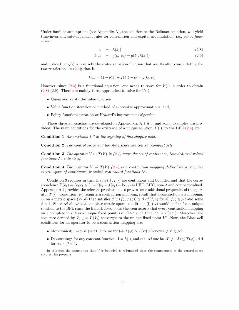
Under familiar assumptions (see Appendix A), the solution to the Bellman equation, will yieldtime-invariant, sate-dependent rules for consumtion and capital accumulation, i.e., policy func-tions:
ct = h(kt) (2.8)
kt+1 = g(kt; ct) = g(kt; h(kt)) (2.9)
and notice that g(�) is precisely the state-transition function that results after consolidating thetwo restrictions in (2.4); that is:
kt+t = (1� �)kt + f(kt)� ct = g(kt; ct)
However, since (2.4) is a functional equation, one needs to solve for V (�) in order to obtain(2.8)-(2.9). There are mainly three approaches to solve for V (�):
� Guess and verify the value function
� Value function iteration or method of successive approximations, and,
� Policy functions iteration or Howard�s improvement algorthm.
These three approaches are developed in Appendixes A.1-A.3, and some examples are pro-vided. The main conditions for the existence of a unique solution, V (�); to the BFE (2.4) are:
Condition 1 Assumptions 1-3 at the begining of this chapter hold.
Condition 2 The control space and the state space are convex, compact sets,
Condition 3 The operator V 7! T (V ) in (2.4) maps the set of continuous, bounded, real-valuedfunctionsM into itself.1
Condition 4 The operator V 7! T (V ) (2.4) is a contraction mapping de�ned on a completemetric space of continuous, bounded, real-valued functionsM.
Condition 3 requires in turn that u (�) ; f (�) are continuous and bounded and that the corre-spondence � (kt) = fctjct � (1� �)kt + f(kt)� kt+1g is UHC, LHC, non-? and compact-valued.Appendix A.4 provides the relevant proofs and also proves some additional properties of the oper-ator T (�) : Condition (iv) requires a contraction mapping; recall that a contraction is a mapping,'; on a metric space (W; d) that satis�es d (' (f) ; ' (g)) � � � d (f; g) for all f; g 2M and some� < 1: SinceM above is a complete metric space, conditions (i)-(iv) would su¢ ce for a uniquesolution to the BFE since the Banach �xed point theorem asserts that every contraction mappingon a complete m.s. has a unique �xed point, i.e., 9 V � such that V � = T (V � ). Moreover, thesequence de�ned by Vi+1 = T (Vi) converges to the unique �xed point V �: Now, the Blackwellconditions for an operator to be a contraction mapping are:
� Monotonicity: ' > (w.r.t. box metric)) T (') > T ( ) whenever '; 2M.
� Discounting: for any constant function A = h(�), and ' 2M one has T ('+A) � T (')+�Afor some � < 1:
1 In this case the assumption that V is bounded is redundand since the compactness of the control spaceensures this property.
11
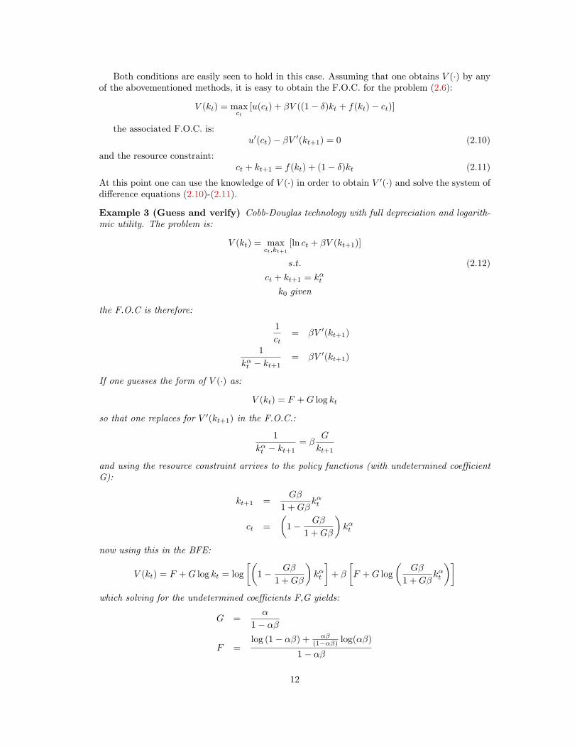
Both conditions are easily seen to hold in this case: Assuming that one obtains V (�) by anyof the abovementioned methods, it is easy to obtain the F.O.C. for the problem (2.6):
V (kt) = maxct[u(ct) + �V ((1� �)kt + f(kt)� ct)]
the associated F.O.C. is:u0(ct)� �V 0(kt+1) = 0 (2.10)
and the resource constraint:ct + kt+1 = f(kt) + (1� �)kt (2.11)
At this point one can use the knowledge of V (�) in order to obtain V 0(�) and solve the system ofdi¤erence equations (2.10)-(2.11).
Example 3 (Guess and verify) Cobb-Douglas technology with full depreciation and logarith-mic utility. The problem is:
V (kt) = maxct;kt+1
[ln ct + �V (kt+1)]
s:t: (2.12)
ct + kt+1 = k�t
k0 given
the F.O.C is therefore:
1
ct= �V 0(kt+1)
1
k�t � kt+1= �V 0(kt+1)
If one guesses the form of V (�) as:
V (kt) = F +G log kt
so that one replaces for V 0(kt+1) in the F.O.C.:
1
k�t � kt+1= �
G
kt+1
and using the resource constraint arrives to the policy functions (with undetermined coe¢ cientG):
kt+1 =G�
1 +G�k�t
ct =
�1� G�
1 +G�
�k�t
now using this in the BFE:
V (kt) = F +G log kt = log
��1� G�
1 +G�
�k�t
�+ �
�F +G log
�G�
1 +G�k�t
��which solving for the undetermined coe¢ cients F,G yields:
G =�
1� ��
F =log (1� ��) + ��
(1���) log(��)
1� ��
12

so that �nally one can generate optimal plans fct; kt+1g1t=1 from the fully speci�ed policy func-tions:
ct = (1� ��) k�tkt+1 = (��) k�t
Finally, note that the transversality condition is satis�ed:
limt!1
�t+1V 0(kt+1)kt+1 = limt!1
�t+1�
�
1� ��
�= 0
2.4.1 The Envelope Theorem approach
A di¤erent avenue that avoids dealing with the value function explicitely is as follows. If con-ditions 1-4 above regarding the objects in the problem are satis�ed (i.e., concavity, convexity,continuity, compactness, monotonicity, discounting), then the unique solution to the BFE V (�),would be continuous, concave, increasing and importantly, di¤erentiable. Hence, the Envelopetheorem applies and one can use the envelope condition for the value function (see the AppendixA for a more elaborate example). To see how the Envelope theorem works in this particularcase, recall the policy functions:
c�t = h (kt)
k�t+1 = g(kt; c�t )
= (1� �)kt + f(kt)� h (kt)
then the value function becomes:
V (kt) = u(h (kt)) + �V ((1� �)kt + f(kt)� h (kt))
di¤erentiating w.r.t. kt :
V 0(kt) =@u(h (kt))
@h (kt)
@h (kt)
@kt+ �V 0 (kt+1)
�(1� � + @f(kt)
@kt� @h (kt)
@kt
�=
@u(h (kt))
@h (kt)
@h (kt)
@kt+ �V 0 (kt+1)
�(1� � + @f(kt)
@kt
�� �V 0 (kt+1)
@h (kt)
@kt
= �V 0 (kt+1)
�(1� � + @f(kt)
@kt
�+@h (kt)
@kt
�@u(h (kt))
@h (kt)� �V 0 (kt+1)
�but the F.O.C. (2.10) implies:
@u(h (kt))
@h (kt)= u0 (ct) = �V 0 (kt+1)
and therefore:
V 0(kt) = �V 0 (kt+1)
�(1� � + @f(kt)
@kt
�= �u0 (ct)
�(1� � + @f(kt)
@kt
�and since this holds for every period:
V 0(kt+1) = u0(ct+1) [f0(kt+1) + (1� �)]
13
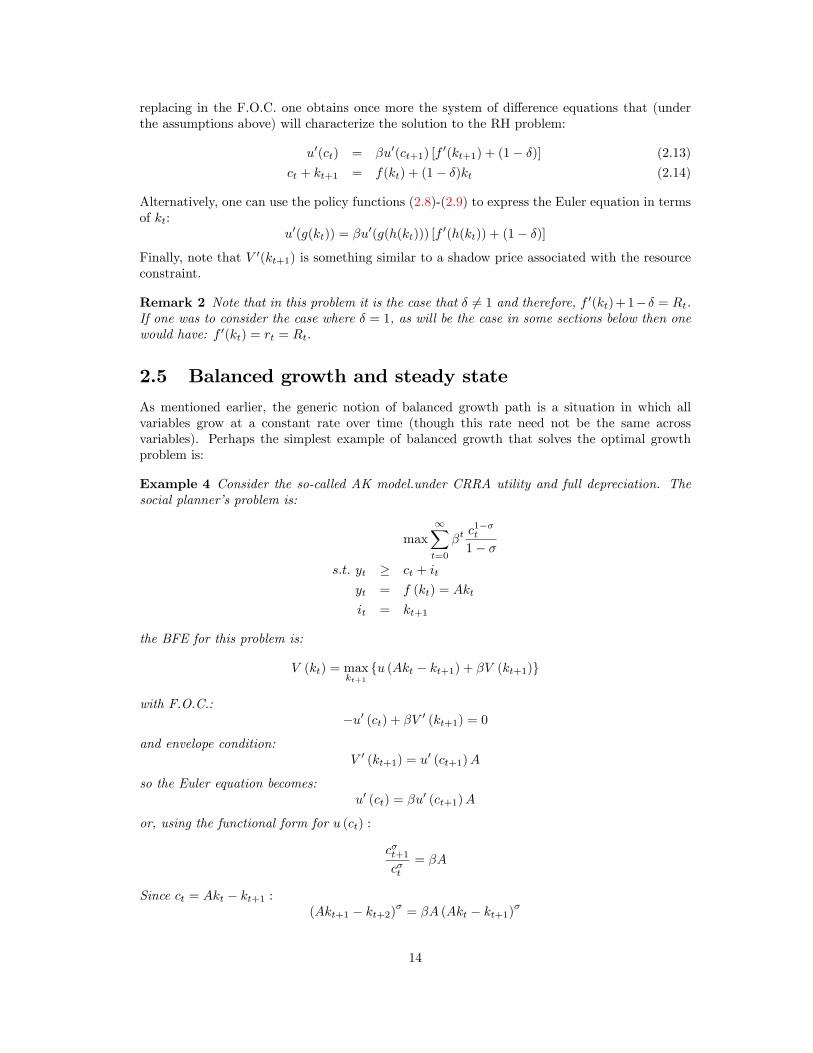
replacing in the F.O.C. one obtains once more the system of di¤erence equations that (underthe assumptions above) will characterize the solution to the RH problem:
u0(ct) = �u0(ct+1) [f0(kt+1) + (1� �)] (2.13)
ct + kt+1 = f(kt) + (1� �)kt (2.14)
Alternatively, one can use the policy functions (2.8)-(2.9) to express the Euler equation in termsof kt:
u0(g(kt)) = �u0(g(h(kt))) [f0(h(kt)) + (1� �)]
Finally, note that V 0(kt+1) is something similar to a shadow price associated with the resourceconstraint.
Remark 2 Note that in this problem it is the case that � 6= 1 and therefore, f 0(kt)+1� � = Rt.If one was to consider the case where � = 1, as will be the case in some sections below then onewould have: f 0(kt) = rt = Rt:
2.5 Balanced growth and steady state
As mentioned earlier, the generic notion of balanced growth path is a situation in which allvariables grow at a constant rate over time (though this rate need not be the same acrossvariables). Perhaps the simplest example of balanced growth that solves the optimal growthproblem is:
Example 4 Consider the so-called AK model.under CRRA utility and full depreciation. Thesocial planner�s problem is:
max1Xt=0
�tc1��t
1� �s:t: yt � ct + it
yt = f (kt) = Akt
it = kt+1
the BFE for this problem is:
V (kt) = maxkt+1
fu (Akt � kt+1) + �V (kt+1)g
with F.O.C.:�u0 (ct) + �V 0 (kt+1) = 0
and envelope condition:V 0 (kt+1) = u0 (ct+1)A
so the Euler equation becomes:u0 (ct) = �u0 (ct+1)A
or, using the functional form for u (ct) :
c�t+1c�t
= �A
Since ct = Akt � kt+1 :(Akt+1 � kt+2)� = �A (Akt � kt+1)�
14

A second order di¤erence equation that, without a (on k) that, without a terminal condition hasmultiple solutions for any given k0: The interest is in that which satis�es the TVC (2.7) whichin this case becomes (using the EC):
limt!1
�t+1V 0 (kt+t) kt+1 = limt!1
�t+1u0 (ct+1)Akt+1
Now to �nd conditions that ensure holding of the TVC note that in a BGP capital and consump-tion grow at the same constant rate so kt+1 = kt and ct+1 = ct for some : Thus:
( ct)�
c�t= �A) = (�A)
1=�
which brings positive growth iif � > 1=A. Next, rewrite u0 (ct+1) = c��t =�A and kt+1 = t+1k0in the TVC:
limt!1
�t+1u0 (ct+1)Akt+1 = limt!1
�t+1c��t�A
A t+1k0
= limt!1
�t+1c��t� t+1k0
= limt!1
(� )tc��t k0
then the TVC holds iif � < 1 )if � (�A)1=� < 1: Hence by assuming that � < A�1
1+� one canensure that there is balanced growth and the TVC holds.
A special case of a balanced growth path is a steady state, in which the growth rate of allvariables is equal to zero. From (2.13)-(2.14) one can compute the steady state by noting thatin the SS, xt = xt+1 = x� for x = fc; k; yg. Hence:
u0(�c) = �u0(�c)�f 0(�k) + (1� �)
�1
�= f 0(�k) + (1� �)
de�ning a modi�ed golden rule for capital accumulation, and
�c� ��k = f(�k) = �y
2.6 Linearization
Next it is possible to study the behavior of the model around the steady state (SS). Recall thatin the SS, xt = xt+1 = �x for x = [c; k]0 and xt = (xt � �x)=�x . So, linearize the system aroundthe SS. Recall that to linearize G(x; y) = 0 around the SS (�x; �y):�
@G
@xt(�x; �y)�x
�xt +
�@G
@yt(�x; �y)�y
�yt = 0
Linearizing (2.13):�ct = �ct+1 + kt+1 (2.15)
where division by u0(�c) on both sides has been used and the fact that 1=� = f 0(�k)+ (1� �) fromthe SS and �; are the elasticities of u0(�) and f 0(�), respectively. Finally, the linear constraintis linearized as:
�cct + �kkt+1 =�f(�k) + (1� �)
��kkt
!ct + �kt+1 = [� + ! + � � 1] kt (2.16)
15

where ! = �c�y , � =
�k�y and � is the elasticity of f(�):Now one can suppose that the linearized policy
functions are of the form:
ct = �1kt
kt+1 = �2kt
so that replacing in (2.15)-(2.16) one obtains:
��1 = ��1�2 + �2
!�1 + ��2 = [� + ! + � � 1]
and one can solve for the undetermined coe¢ cients �1; �2 as functions of parameters ofthe model (�; !; �). Note that the �rst of these equations will be a cuadratic one so one hastwo solutions, from which one selects �2 < 1 since this is the only solution that satis�es thetransversality condition. With this log-linear policy functions and the "true" coe¢ cients asfunctions of the parameters of the model, one can generate optimal sequences fct; kt+1g1t=0, thatis sequences of the variables in deviation from SS form.
2.7 Equilibrium growth and welfare theorems
The solution to the optimal growth model can in fact be deduced as the outcome of a competitiveequilbrium. To see this, state the problem of the RH and the �rm separately.
Households
The representative household maximizes lifetime discounted utility subject to its resource con-straint. Households own the factors of production k; l and own the �rms. For simplicity, supposethere is full depreciation (� = 1). At each period, the RH receives income from renting all of itsavailable capital, working all its endowed labor and earning pro�ts from the �rms.2 With thisincome, the RH and decides how much to consume and how much to invest (save):
maxct
1Xt=0
�tu(ct)
s:t:
ct + kht+1 � rtk
ht + wtl
ht + �t = yht
Firms
Firms produce a single good by renting production factors from the RH and maximize pro�tssubject to their production technology:
max1Xt=0
�t = max1Xt=0
�pty
ft � wtl
ft � rtk
ft
�s:t:
yft � F (kft ; lft )
where F (�) is continuous, di¤erentiable, strictly increasing and homogeneous of degree one. Sincethere is only one good in the economy, there are no relative prices and one can set pt = 1. Also,
2The assumption that households work their entire endowment of labor re�ects the fact that there is nodisutility of labor in this model. The RBC models surveyed in the sections below relax this assumption so thatlabor becomes in fact a choice variable.
16

since there is no discounting, lifetime pro�ts are maximized , pro�ts are maximized at everyperiod t:3
Equilibrium
For simplicity suppose that lht = 1: Then a competitive equilibrium consists of a set of pricesfpt = 1; wt; rtg1t=0 and allocations fk�t ; l�t = 1; y�t ; c�t g
1t=0 such that 8 t :
1. The �rm maximizes pro�ts. To do so, note that since F (�) is strictly increasing, thetechnology constraint will hold with equality
�yft = F (kft ; l
ft )�. Thus, the F.O.C.s of the
�rm are:
@�(kft ; lft )
@lft= 0 =) wt = Fl(k
ft ; l
ft )
@�(kft ; lft )
@kft= 0 =) rt = Fk(k
ft ; l
ft )
2. The RH maximizes utility. The F.O.C.s for the RH are, as before:
u0(ct) = �u0(ct+1)rt+1
ct + kht+1 = rtk
ht + wtl
ht + �t
3. Markets clear in all periods (t = 1; 2:::):
yht = yft = F (kft ; lft )
lht = lft = 1
kht = kft
Next, replace the F.O.C.s for the �rm in the pro�t function at t and recalling that lt = 1:
�t = F (k�t ; l�t )� Fl(k�t ; l�t )� Fk(k�t ; l�t )k�t
and because F (�) is homogeneous of degree one, Euler�s theorem (x �rf(x) = f(x)) impliesthat �t = 0 so that:
wt = F (k�t ; l�t )� Fk(k�t ; l�t )k�t
andP1
t=0 �t = 0 . Replacing in the F.O.C.s for the RH yields:
u0(ct) = �u0(ct+1)Fk(k�t ; l
�t )
and
ct + k�t+1 = Fk(k
�t ; l
�t )k
�t + F (k
�t ; l
�t )� Fk(k�t ; l�t )k�t
= F (k�t ; l�t )
which are of course, the same optimality conditions derived under the centralized approach inthe section above. Hence one has found a vector of prices that delivers the (planned) Paretooptimal allocation which results as a solution to (2.13)-(2.14). That is, the optimal allocationhas been �descentralized�as a competitive equilibrium of the economy This is an ilustration ofthe second fundamental theorem of welfare economics. 4
.3 It is straightforward to extend this model to the case where �rms discount future pro�ts. A natural candidate
for discounting would be 1Rwhere R is the gross interest rate (in this economy all assets would earn R).
4Recall that the �rst welfare theorem states that whenever households are non-satiated, a competitive equi-librium allocation is Pareto optimal.
17

2.8 Extensions to the optimal growth model
2.8.1 Assets in the OGM
Recall the budget constraint for the RH is, in general:
kt+1 = (1 + rt � �)kt + wtlt + �t � ct
and if one assumes lt = 1 8 t:
kt+1 = (1 + rt � �)| {z } kt + wt � ct + �t (2.17)
Rt = gross return
Now, allow for assest at that HH carry from previous periods. Note that in aggregate at = kt+btwhere we may have bt < 0 at some t. So we can re-write the �ow budget constraint as:
ct + at+1 = Rtat + wt + �tctRt+at+1Rt
= at + wt + �t
At this point one carries out forward substitution of at+1 from the equation for at+2, then sub-stitute the latter from the equation for at+3 and so on. For some �nite T � 1; the intertemporalbudget constraint (IBC) is given by:
TXt=0
1
Rtct +
aT+1RT
= (1 + r0 � �)a0 +TXt=0
1
Rt(wt + �t) (2.18)
where:
Rt =tY
j=1
Rj =tY
j=1
(1 + rj � �)
But since we�re assuming an in�nite horizon, we must prevent aT+1RT ! �1 as T !1 (builddebt forever) which would result in
P1t=0
1Rt ct ! 1: So we impose the additional no Ponzi
games condition:limT!1
aT+1RT
= 0
so that when the horizon is in�nite, taking limits on both sides of (2.18) and using the no-Ponzicondition, the IBC can be expressed as:
1Xt=0
1
Rtct| {z } = (1 + r0 � �)a0| {z } +
1Xt=0
1
Rt(wt + �t)| {z } (2.19)
PV consumption = initial asset income + PV non-asset income
Note that a stream of consumption that satis�es the (IBC) also satis�es the �ow constraint ateach t. To see this, consider a consumption plan fctg1t=0 that satis�es the IBC. At some � , by(2.18) the household will have accumulated assets:
a�+1R�
= (1 + r0 � �)a0 +�Xt=0
1
Rt(wt + �t � ct)
= (1 + r0 � �)a0 +��1Xt=0
1
Rt(wt + �t � ct) +
1
R�(w� + �� � c� ) (2.20)
18
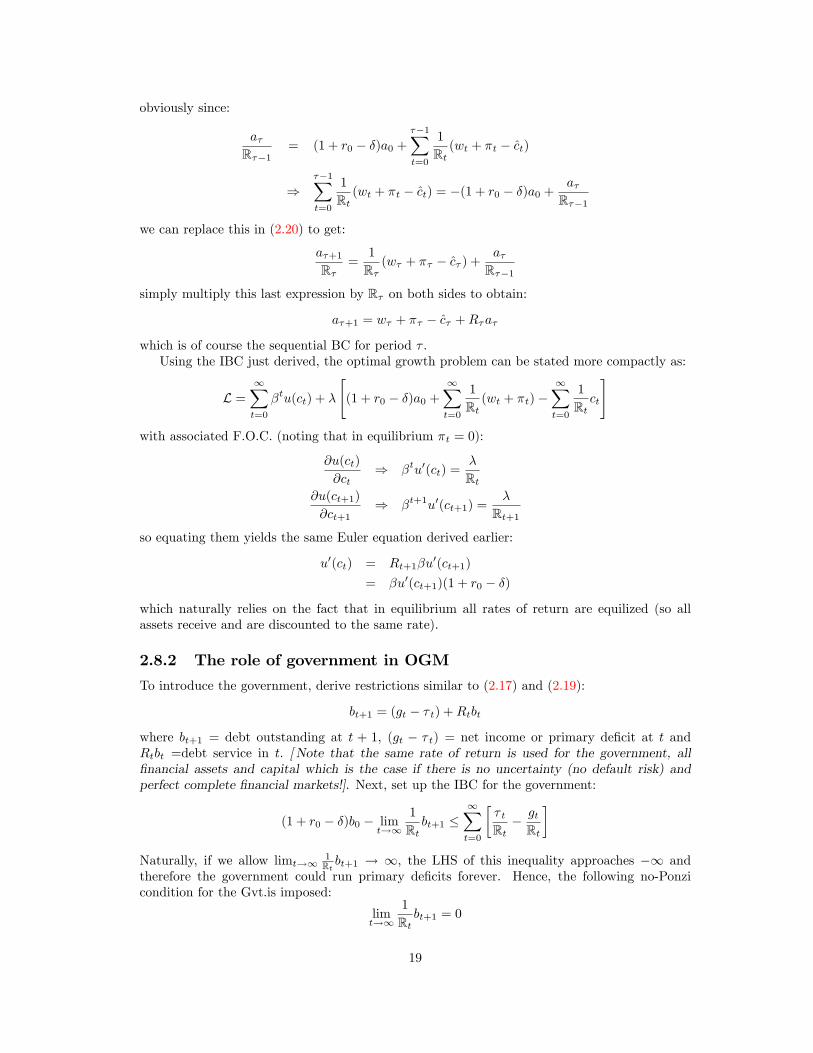
obviously since:
a�R��1
= (1 + r0 � �)a0 +��1Xt=0
1
Rt(wt + �t � ct)
)��1Xt=0
1
Rt(wt + �t � ct) = �(1 + r0 � �)a0 +
a�R��1
we can replace this in (2.20) to get:
a�+1R�
=1
R�(w� + �� � c� ) +
a�R��1
simply multiply this last expression by R� on both sides to obtain:
a�+1 = w� + �� � c� +R�a�
which is of course the sequential BC for period � .Using the IBC just derived, the optimal growth problem can be stated more compactly as:
L =1Xt=0
�tu(ct) + �
"(1 + r0 � �)a0 +
1Xt=0
1
Rt(wt + �t)�
1Xt=0
1
Rtct
#with associated F.O.C. (noting that in equilibrium �t = 0):
@u(ct)
@ct) �tu0(ct) =
�
Rt@u(ct+1)
@ct+1) �t+1u0(ct+1) =
�
Rt+1so equating them yields the same Euler equation derived earlier:
u0(ct) = Rt+1�u0(ct+1)
= �u0(ct+1)(1 + r0 � �)
which naturally relies on the fact that in equilibrium all rates of return are equilized (so allassets receive and are discounted to the same rate).
2.8.2 The role of government in OGM
To introduce the government, derive restrictions similar to (2.17) and (2.19):
bt+1 = (gt � � t) +Rtbt
where bt+1 = debt outstanding at t + 1, (gt � � t) = net income or primary de�cit at t andRtbt =debt service in t: [Note that the same rate of return is used for the government, all�nancial assets and capital which is the case if there is no uncertainty (no default risk) andperfect complete �nancial markets!]. Next, set up the IBC for the government:
(1 + r0 � �)b0 � limt!1
1
Rtbt+1 �
1Xt=0
�� tRt� gtRt
�Naturally, if we allow limt!1
1Rt bt+1 ! 1, the LHS of this inequality approaches �1 and
therefore the government could run primary de�cits forever. Hence, the following no-Ponzicondition for the Gvt.is imposed:
limt!1
1
Rtbt+1 = 0
19
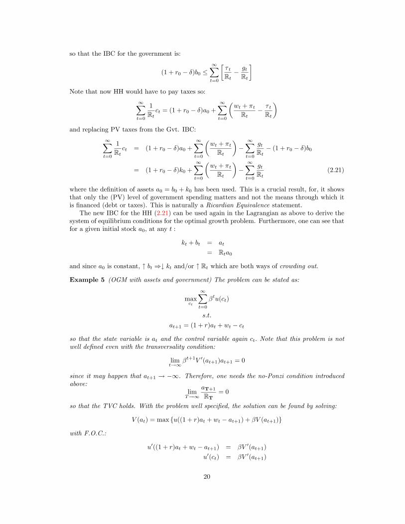
so that the IBC for the government is:
(1 + r0 � �)b0 �1Xt=0
�� tRt� gtRt
�Note that now HH would have to pay taxes so:
1Xt=0
1
Rtct = (1 + r0 � �)a0 +
1Xt=0
�wt + �tRt
� � tRt
�and replacing PV taxes from the Gvt. IBC:
1Xt=0
1
Rtct = (1 + r0 � �)a0 +
1Xt=0
�wt + �tRt
��
1Xt=0
gtRt� (1 + r0 � �)b0
= (1 + r0 � �)k0 +1Xt=0
�wt + �tRt
��
1Xt=0
gtRt
(2.21)
where the de�nition of assets a0 = b0 + k0 has been used. This is a crucial result, for, it showsthat only the (PV) level of government spending matters and not the means through which itis �nanced (debt or taxes). This is naturally a Ricardian Equivalence statement.The new IBC for the HH (2.21) can be used again in the Lagrangian as above to derive the
system of equilibrium conditions for the optimal growth problem. Furthermore, one can see thatfor a given initial stock a0, at any t :
kt + bt = at
= Rta0
and since a0 is constant, " bt )# kt and/or " Rt which are both ways of crowding out.
Example 5 (OGM with assets and government) The problem can be stated as:
maxct
1Xt=0
�tu(ct)
s:t:
at+1 = (1 + r)at + wt � ct
so that the state variable is at and the control variable again ct: Note that this problem is notwell de�ned even with the transversality condition:
limt!1
�t+1V 0(at+1)at+1 = 0
since it may happen that at+1 ! �1. Therefore, one needs the no-Ponzi condition introducedabove:
limT!1
aT+1RT
= 0
so that the TVC holds. With the problem well speci�ed, the solution can be found by solving:
V (at) = max fu((1 + r)at + wt � at+1) + �V (at+1)g
with F.O.C.:
u0((1 + r)at + wt � at+1) = �V 0(at+1)
u0(ct) = �V 0(at+1)
20

and envelope condition:
V 0(at+1) = u0((1 + r)at+1 + wt � at+2)(1 + r)= u0(ct+1)(1 + r)
and the usual Euler equation:u0(ct) = �u0(ct+1)(1 + r)
2.9 Optimal Growth in continuous time
State the problem (2.1) in continuous time:
maxc(t);I(t)
1Z0
u(c(t))e��tdt
s:t: (2.22)
c(t) + i (t) � f(k(t))
_k(t) = i (t)� �k(t) (2.23)
k(0) given
The continuous time problem is actually easier to solve using the tools of optimal control; areview of The Maximum Principle and the Hamiltonian approach is presented in Appendix B.Set up the (present-value) Hamiltonian:
H = u(c(t))e��t + �(t) [f(k(t))� �k(t)� c(t)] (2.24)
where �(t) is the co-state variable. The condition for c(t) to maximize the Hamiltonian is:
i)@H
@c(t)= 0 =) u0(c(t))e��t = �(t) (2.25)
solving this yelds c�(t) as a function of the co-state and parameters. Next, we can replace c�(t)in (2.24) to obtain the maximum value function of the Hamiltonian, H�, di¤erentiate w.r.t. stateand co-state variables. Alternatively, simply state the Pontryagin conditions similar to thosederived in the Appendix B (B.8)-(B.9):
ii) _�(t) = � @H
@k(t)= ��(t) [f 0(k(t))� �] (2.26)
iii) _k(t) =@H
@�(t)= f(k(t))� �k(t)� c(t) (2.27)
Conditions (2.25)-(2.26)-(2.27) along with the TCV:
limt!1
�(t)k(t) = 0
are the three di¤erential equations (and terminal condition) that characterize the solution tothe HH problem.
Example 6 Suppose that u (c (t)) = ln (c (t)). Then from (2.25):
c(t) =e��t
�(t)
21

so that replacing in (2.27) we get the two di¤erential equations on k and � that characterize thesolution:
_k(t) = f(k(t))� �k(t)� e��t
�(t)
_�(t) = ��(t) [f 0(k(t))� �]
Alternatively, one can solve the system in terms of di¤erential equations in c and k, which ismore consistent with the idea of policy rules described in previous sections. To do so, di¤erentiate(2.25) w.r.t. time:
u00(c(t))e��t _c(t)� �e��tu0(c(t)) = _�(t) (2.28)
and replace in (2.26) to obtain:
u00(c(t))e��t _c(t)� �e��tu0(c(t)) = ��(t) [f 0(k(t))� �]u00(c(t))e��t _c(t)� �e��tu0(c(t)) = �e��tu0(c(t)) [f 0(k(t))� �]
which upon rearranging:_c(t)
c(t)=
f 0(k(t))� � � �� [c(t)u00(c(t))=u0(c(t))] (2.29)
where the denominator is naturally, the Arrow-Pratt CRRA coe¢ cient: This condition tells usthat whenever f 0(k(t)) is "large", which happens when k(t) is "low", we have _c=c > 0 so thatthe HH consumes less today and more in the future. Likewise, _c=c < 0 if � is large enough whichsuggests that the HH is more "patient".Finally, the TVC is:
limt!1
�(t)k(t) = 0
limt!1
e��tu0(c(t))k(t) = 0
2.9.1 Steady State
Recall, in SS _c(t) = 0 and _k(t) = 0. Therefore:
_c(t)
c(t)= 0 =) f 0(�k)� � = � (2.30)
which is, again, a modi�ed Golden Rule for capital accumulation and, once more, independentfrom the shape of u(�): Next:
_k(t) = 0 =) f(�k)� �c = ��k
so that SS-investment just breaks-even (making _k(t) = 0).
Remark 3 Note that �(t) is the shadow price of capital, i.e., it measures the impact of a smallincrease in kt on the optimal value of the program. By comparison, V (kt) is the value of of theoptimal program from t given the level of capital kt: Therefore, we have that:
�(t) = V 0(kt)
and note that _�(t) represents the appreciation of capital since its the change in the value of aunit of the state variable.
Exercise 7 In order to make meaningful comparisons with the Solow model, reintroduce techni-cal change and poppulation growth. (i) Write the equilibrium conditions of the OGM considerngthese features and (ii) Show that along the balanced growth path, �k < �kGold where �kGold is theGolden Rule level of (per-e¤ective-labor) capital in the Solow model.
22
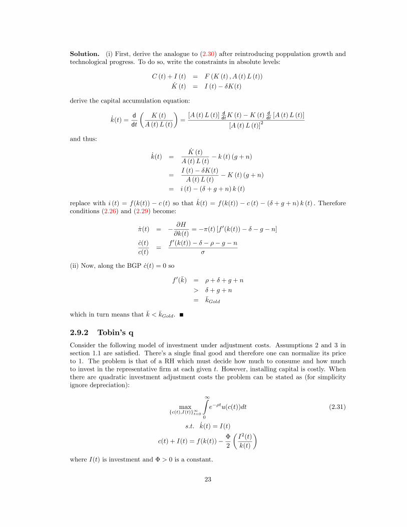
Solution. (i) First, derive the analogue to (2.30) after reintroducing poppulation growth andtechnological progress. To do so, write the constraints in absolute levels:
C (t) + I (t) = F (K (t) ; A (t)L (t))_K (t) = I (t)� �K(t)
derive the capital accumulation equation:
_k(t) =d
dt
�K (t)
A (t)L (t)
�=[A (t)L (t)] ddtK (t)�K (t)
ddt [A (t)L (t)]
[A (t)L (t)]2
and thus:
_k(t) =_K (t)
A (t)L (t)� k (t) (g + n)
=I (t)� �K(t)A (t)L (t)
�K (t) (g + n)
= i (t)� (� + g + n) k (t)
replace with i (t) = f(k(t)) � c (t) so that _k(t) = f(k(t)) � c (t) � (� + g + n) k (t) : Thereforeconditions (2.26) and (2.29) become:
_�(t) = � @H
@k(t)= ��(t) [f 0(k(t))� � � g � n]
_c(t)
c(t)=
f 0(k(t))� � � �� g � n�
(ii) Now, along the BGP _c(t) = 0 so
f 0(�k) = �+ � + g + n
> � + g + n
= �kGold
which in turn means that �k < �kGold:
2.9.2 Tobin�s q
Consider the following model of investment under adjustment costs. Assumptions 2 and 3 insection 1.1 are satis�ed. There�s a single �nal good and therefore one can normalize its priceto 1. The problem is that of a RH which must decide how much to consume and how muchto invest in the representative �rm at each given t. However, installing capital is costly. Whenthere are quadratic investment adjustment costs the problem can be stated as (for simplicityignore depreciation):
maxfc(t);I(t)g1t=0
1Z0
e��tu(c(t))dt (2.31)
s:t. _k(t) = I(t)
c(t) + I(t) = f(k(t))� �2
�I2(t)
k(t)
�where I(t) is investment and � > 0 is a constant:
23

Note that in this problem, the control variables are c(t) and I(t) (or kt+1 in the OGM), whilethe state variable is k(t). On what follows, the present-value optimization problem is solvedand then it is expressed in current value terms since the latter form lends itself to intuitiveinterpretation. First, we get rid of c(t) by using the second constraint. Notice that we can dothis only because the constraint is speci�ed with equality. Notice also that after eliminating thisconstraint, the Lagrangian and the Hamiltonian are obviously the same so that in the languageof Appendix B, G (�) dissapears and LI = HI : Thus, set up the present-value Hamiltonian:
Hpv = e��tu
�f(k(t))� I(t)� �
2
�I2(t)
k(t)
��+ �(t)I(t)
The F.O.C. w.r.t. the control is simply obtained:
�(t) = e��tu0 (c (t))
�1 + �
�I(t)
k(t)
��(2.32)
Next, using the Pontryagin conditions corresponding to the present-value problem (B.8)-(B.9):
_�(t) = �e��tu0 (c (t))"f 0(k(t)) +
�
2
�I(t)
k(t)
�2#(2.33)
_k(t) = I(t) (2.34)
Or, using the F.O.C. to solve for I (t) we can rewrite (2.34) as:
_k(t) =k (t)
�
�e�t�(t)
u0 (c� (t))� 1�
And just as in the discrete time problem, the TVC is given by: limt!1 �(t)k(t): Naturally,with an explicit functional form for u, we could solve for c� (t) ; I� (t) using the F.O.C. (2.32)and the constraint, replace this in (2.33)-(2.34) to obtain a pair of di¤erential equations on �(t)and k(t) that would characterize the solution to the problem.An interesting avenue to take in this problem is to express the equilibrium conditions in
current-value terms. To do so, multiply (2.33) by e�t on both sides (the other conditions donot involve �(t)) and de�ne q(t) = e�t�(t). Then, since _q(t) = _�(t)e�t + ��(t)e�t, one has that_�(t)e�t = _q(t)� �q(t) and therefore the Pontryagin conditions can be written:
_q(t)� �q(t) = �u0 (c (t))"f 0(k(t)) +
�
2
�I(t)
k(t)
�2#(2.35)
_k(t) =k (t)
�
�q(t)
u0 (c� (t))� 1�
(2.36)
Finally, using (2.35) we can arrive at:
_q(t)� �q(t) = �u0 (c (t))"f 0(k(t)) +
�
2
�I(t)
k(t)
�2#
q(t) =
Z 1
t
e��(s�t)u0(c(s))| {z }24f 0(k(t)) + �
2
�I(t)
k(t)
�2| {z }
35 dsdisc. marg. util of output � marg. prod. of k - marg. adj cost (2.37)
that is, Tobin�s q summarizes the informarion of the discounted social bene�t of installing anadditional unit of capital.
24
Chapter 3
Overlapping generations (OLG)
3.1 OLG in economies with production (Diamond�s)
Assume that a generation is born in every period of time. Time is discrete indexed t = 1; 2:::Each generation lives two periods. Therefore, at each t, there are two generations alive; "younghouseholds" and "old households", call them HH types 1 and 2. For completeness, suppose thatat period t = 1 a generation is already alive (agent type 0). Therefore generation t is that bornin period t: Each new generation is larger than the previous one by a factor of (1+n), n 2 (0; 1).Therefore:
Lt = (1 + n)Lt�1
In its �rst year of life, each HH works, saves and consumes. In its second year of life each HHonly consumes. Therefore:
c1;t ! period t consumption of a typical HH from generation t ("youngs")
c2;t+1 ! period t+ 1 consumption of a typical HH from generation t ("olds")
Production is carried out by the use of capital, technology and "young" agents as the labor forcewith Harrod-neutral production function:
F (Kt; AtLt)
Moreover, production technology satis�es assumptions 1)-3) in section 1.1 and utility satis�esassumptions 2)-4) in section 2.2. Technology follows an exogenous growth process:
At = (1 + g)At�1
Hence, there are three markets; �nal goods, capital goods and labor. Markets are competitiveand for simplicity, there is full depreciation (� = 1). Acordingly, �t = 0, FK = 1 + rt = Rt andFL = wt: In period t, each HH from generation t works, receives (technology-enhanced) laborincome, consumes and saves1 :
Atwt = c1;t + st
Generation t�s savings are rented in the form of capital for production at t + 1 so that capitalavailable is:
Kt+1 = Ltst = St (3.1)
1Since only "youngs" save on each period, there is no s2;t ("olds" don�t save), to simplify notation st =s1;t =total savings of the economy at t:
25

and are returned with the corresponding rental income. Generation t (i.e. agent type 2 in periodt+ 1) then consumes the proceedings:
c2;t+1 = Rt+1st
= (1 + rt+1)st
= (1 + rt+1) (Atwt � c1;t)
Generation t then maximizes its (discounted) lifetime utility from consumption:
maxc1;t;c2;t+1
U(c) = u(c1;t) + �u(c2;t+1) (3.2)
s:t:
Atwt = c1;t +c2;t+1Rt+1
(3.3)
alternatively, one the RH solves the unconstrained optimization problem:
maxc1;t
U(c) = u(c1;t) + �u(Rt+1(Atwt � c1;t))
both yielding the same F.O.C. and Euler equation:
u0(c1;t) = �u0(c2;t+1)Rt+1 (3.4)
which is analogous to the one found in the OGM. Equations (3.3)-(3.4) are the pair of di¤erenceequations describing the solution to the typical generation t HH problem. Next, note that theEuler equation can be expressed as:
u0(c1;t) = �(�; u0(c2;t+1); Rt+1)
and that u00 < 0) u0�1(c1;t) = c1;t. Therefore:
u0�1(c1;t) = u0�1(c2;t+1) ���1(�; u0(c2;t+1); Rt+1)c1;t = u0�1(c2;t+1) ���1(�; u0(c2;t+1); Rt+1)
hence, if one replaces in:
Atwt = c1;t + st
st = Atwt � u0�1(c2;t+1) ���1(�; u0(c2;t+1); Rt+1)st = (Atwt; Rt+1)
(+) (?)
where is called the savings function. Consider a rise in labor income Atwt, then, everythingelse constant, the properties of u (�) imply that consumption in both periods would rise, whichimplies that st increases; thus the sign of @st=@Atwt is unambiguous. However, consider a risein Rt+1. There are two e¤ects to consider. First, since the opportunity cost of consumptionin t rises, the HH may want to substitute current for future consumption (substitution e¤ect).Second, a rise in Rt+1 has an income e¤ect since each unit saved yields higher return so theHH will want to consume more on both periods. The total e¤ect is ambiguous as is the sign of@st=@Rt+1:Next, to derive the law of motion of capital come back to (3.1):
Kt+1 = Ltst = St
Kt+1 = Lt(Atwt; Rt+1)
= Lt(Atwt; FK)
26
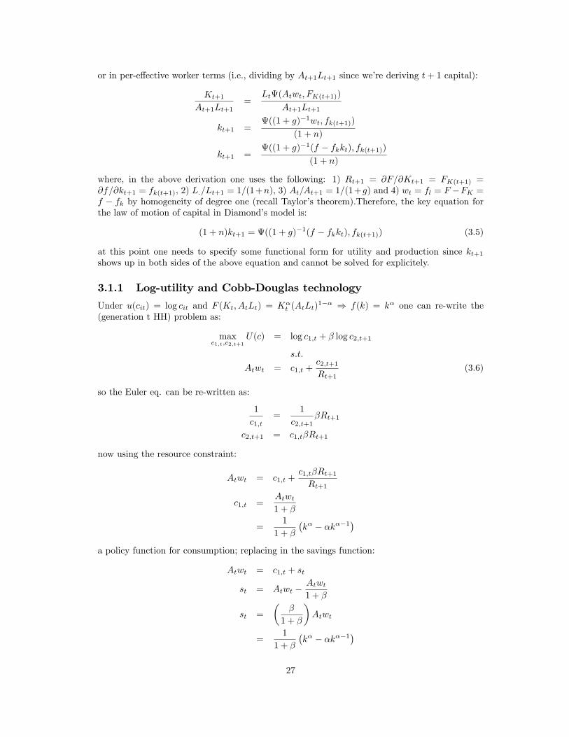
or in per-e¤ective worker terms (i.e., dividing by At+1Lt+1 since we�re deriving t+ 1 capital):
Kt+1
At+1Lt+1=
Lt(Atwt; FK(t+1))
At+1Lt+1
kt+1 =((1 + g)�1wt; fk(t+1))
(1 + n)
kt+1 =((1 + g)�1(f � fkkt); fk(t+1))
(1 + n)
where, in the above derivation one uses the following: 1) Rt+1 = @F=@Kt+1 = FK(t+1) =@f=@kt+1 = fk(t+1), 2) L:=Lt+1 = 1=(1+n), 3) At=At+1 = 1=(1+g) and 4) wt = fl = F �FK =f � fk by homogeneity of degree one (recall Taylor�s theorem):Therefore, the key equation forthe law of motion of capital in Diamond�s model is:
(1 + n)kt+1 = ((1 + g)�1(f � fkkt); fk(t+1)) (3.5)
at this point one needs to specify some functional form for utility and production since kt+1shows up in both sides of the above equation and cannot be solved for explicitely.
3.1.1 Log-utility and Cobb-Douglas technology
Under u(cit) = log cit and F (Kt; AtLt) = K�t (AtLt)
1�� ) f(k) = k� one can re-write the(generation t HH) problem as:
maxc1;t;c2;t+1
U(c) = log c1;t + � log c2;t+1
s:t:
Atwt = c1;t +c2;t+1Rt+1
(3.6)
so the Euler eq. can be re-written as:
1
c1;t=
1
c2;t+1�Rt+1
c2;t+1 = c1;t�Rt+1
now using the resource constraint:
Atwt = c1;t +c1;t�Rt+1Rt+1
c1;t =Atwt1 + �
=1
1 + �
�k� � �k��1
�a policy function for consumption; replacing in the savings function:
Atwt = c1;t + st
st = Atwt �Atwt1 + �
st =
��
1 + �
�Atwt
=1
1 + �
�k� � �k��1
�27
that is, as in the growth models of the sections above, savings are a constant fraction of HHincome. Next, using the equation for capital:
(1 + n)kt+1 =stAt+1
=1
At+1
��
1 + �
�Atwt
=
��
(1 + �) (1 + g)
�wt
=
��
(1 + �) (1 + g)
�(k�t � �k�t )
kt+1 =
��(1� �)
(1 + �) (1 + g)(1 + n)
�k�t (3.7)
a policy function for capital accumulation. Equation (3.7) is the key equation of Diamond�smodel unde log-utility and Cobb-Douglas production.
3.1.2 Steady state
The steady state value for capital can be computed as:
�k =
��(1� �)
(1 + �) (1 + g)(1 + n)
��k�
�k =
��(1� �)
(1 + �) (1 + g)(1 + n)
� 11��
(3.8)
steady state output, is:
�y = �k�
=
��(1� �)
(1 + �) (1 + g)(1 + n)
� �1��
To obtain SS consumption �rst note that cit is the amount consumed by one typical householdof generation i in its �rst year of life. Since now the poppulation size is not normalized to 1 asin the growth models of previous sections, in order to �nd economy-wide consumption at t onemust compute:
Ct = Ltc1t + Lt�1c2t
so that total consumption per (e¤ective) worker in period t:
ct = c1t +c2t
(1 + n)
now, using:
Ct = Yt � Stct = yt � st�c = �k� � (1 + n)�k
so that:
�c =
��(1� �)
(1 + �) (1 + g)(1 + n)
� �1��
� (1 + n)�
�(1� �)(1 + �) (1 + g)(1 + n)
� 11��
28
3.1.3 Golden rule and dynamic ine¢ ciency
As before, the golden rule for capital accumulation will follow:
�kGold = argmax�k
��k� � (1 + n)�k| {z }
�=�c
with F.O.C. as:
��k��1 = 1 + n
�kGold =
�1 + n
�
� 1��1
(3.9)
or, in the general case:
f 0(�kGold) = 1 + n
R = 1 + n
r = n
that is, only when the interest rate equals the rate of poppulation growth, capital is at its goldenrule level.2
The possibility of dynamic ine¢ ciency arises by comparing (3.8) with (3.9):
�k?= �kGold�
�(1� �)(1 + �) (1 + g)(1 + n)
� 11��
?=
�1 + n
�
� 1��1
therefore, if �k 6= �kGold the current allocation of resources would be Pareto ine¢ cient and theplanner could make every one else by rising/lowering investment (savings)
3.1.4 The role of Government.
Suppose that for some reason the economy �nds itself under dynamic ine¢ ciency, i.e., �k > �kGold.Then the Government could reallocate resources as follows: spend Gt and fund it entirely with(lump-sum) taxes in that same period. Then key equation (3.7) becomes:
kt+1 =
��(1� �)
(1 + �) (1 + g)(1 + n)
�[k�t �Gt]
which unambiguously leads to a lower �k: The intuition is as follows: since the taxes are only on t,then generation t is taxed only on its �rst year of life. The HH would have to reduce consumptionin its �rst period but since it wants to smooth consumption (under CRRA) it would have toreduce its savings too, so that consumption in period t falls less than the full amount of taxes.Consequently, savings fall and the economy moves towards �kGold (which maximizes the SS levelof consumption). The Government in turn can reallocate the taxes as Gt to increase consumptionof those hurt and therefore increase economy-wide consumption.
Claim 8 In the OLG presented above, the Ricardian equivalence result does not hold in general.2Note that if � 6= 1 then this condition becomes (1 + r � �) = 1 + n or r � � = n:
29
To se why, suppose that in period t; Government purchases Gt are introduced and funded byissuing one-period bonds bt = Gt. In turn, in period t+1 the government levies a tax in order torepay for the bonds, so � t+1 = (1 + rt+1)bt: In the OGM the RH would then save whatever thegovernment spends Gt, so that it yields reutrn (1+ rt+1)Gt = � t+1. Therefore, the consumptionplan operates as if the government was funding its purchases via taxes in period t: Hence, theirrelevance of distinguishing between taxes and bonds. On the other hand, in the OLG model,at period t only the young agents care about future taxes; therefore, introducing Gt has reale¤ects on the consumption plan of generation t� 1:
3.1.5 Social security
Consider the problem of social security in the OLG model. "Old" HH receive bene�ts bt thatare funded by some sort of contriubution d: There are two systems; fully funded social securityand pay-as-you-go (PAYGO).Fully funded social security. A HH of generation t contributes d in its �rst period of
life, this contribution is invested at market rates and then in its second period of life the HHreceives (1 +Rt)d: The HH therefore faces the problem3 :
maxc1t;c2t+1
u(c1t) + �u(c2t+1) (3.10)
s:t:
c1;t + st + d � Atwt (3.11)
c2;t+1 � Rt+1(d+ st) (3.12)
Claim 9 Under the above assumptions and de�nitions, the HH problem with fully funded socialsecurity is equivalent to the simple HH problem (3.2)-(3.3) of section 3.1
Proof. To see why, �rst solve for st in the constraint (3.12):
c2;t+1 = Rt+1(dt + st)
st =c2;t+1Rt+1
� d
and next replace in constraint (3.11):
c1;t + st + d = Atwt
c1;t +
�c2;t+1Rt+1
� d�+ d = Atwt
c1;t +c2;t+1Rt+1
= Atwt
which is exactly the resource constraint (3.3). Hence, the problem is identical to that presentedin section 3.1The intuition for this result is simple: if contributions are invested at market rates, then
they are simply a di¤erent way of saving. Therefore, the HH only needs to choose how muchit wants to save at t, then pay d as contributions and invest the remaining as st: Note that,depending on the size of d; it may be optimal for the HH to set st = 0: Also notice that now theamount invested (which matches exactly the amounf of capital available at t+ 1 since � = 1) isst + d = (1 + n)kt+1
3 In this set up it is assumed that each HH of all generations make the same contribution, i.e., the case wheredt 6= dt+1 is ruled out. This possibility is explored in Acemoglu (2008) and in fact the case where dt is a choicevariable is discussed.
30

Pay-as-you-go social security. In this case, a HH from generation t contributes d in its�rst period of life. This amount is transfered in the same period to generation t � 1 (the oldsat t) in the form of bene�ts bt. In its second period of life, each HH of generation t receives thecontributions of generation t+1 HH: bt+1 = (1+n)d: Therefore, the (generation t) HH problemis:
maxc1t;c2t+1
u(c1t) + �u(c2t+1) (3.13)
s:t:
c1;t + st + d � Atwt (3.14)
c2;t+1 � Rt+1st + (1 + n)d (3.15)
so that the consolidated (�ow) resource constraint becomes:
c1;t +
�c2;t+1Rt+1
� (1 + n)Rt+1
d
�+ d � Atwt
therefore, since the return on contributions is now (1 + n) rather than Rt+1 the problem isequivalent to the simple model of 3.1 only if Rt+1 = (1 + n). Also notice that only st goesinto capital accumulation, rather than st + d as before. However, if the economy faces dynamicine¢ ciency and overaccumulation of capital (i.e., Rt+1 < 1 + n) then PAYGO social securityresults in capital accumulation that is lower by d, hence steering the economy again towardsthe golden rule level of capital. Likewise, if d was not �xed but a choice of the HH (or at leasta fraction of it), HH would prefer d to st as long as Rt+1 < 1 + n. This in turn would reducecapital until rates of return again equalize.
3.1.6 Restoring Ricardian equivalence
Suppose the following set up. Instead of new families arriving, assume that each HH beguets(1 + n) o¤springs which count as HH in their second period of life. Therefore, the demographicstructure of the models above remain unchanged. However, suppose now that each HH onlyworks in its second period of life. Moreover, HH consumption on its �rst period of life is incor-porated in its "parent" HH. Finally, the "parent" HH cares about its o¤spring�s consumptionct+1; and therefore considers a bequest bt+1. The problem of generation t� 1 at t is therefore:
maxct;bt+1
u(ct) + �u(ct+1)
s:t: (3.16)
ct + bt+1 � yt � Atwt +Rtbt
where, as before:wt = f(kt)� f 0(kt)kt
and:Rt = f 0(kt)
moreover, assuming � = 1, capital available for production in period t+ 1 equals generation t�swealth in that period, which was bequested to him by its parent HH bt :
Kt+1 = Lt+1bt+1
kt+1 =1
At+1bt+1
At+1kt+1 = bt+1
31

where, Kt+1=Lt+1 is the capital per-worker. Note that the constraint in (3.16) could be re-written as:
ct + bt+1 � At (wt +Rtkt)
Therefore, a HH from generation t� 2 loosens its o¤spring�s resource constraint by bequestingbt. Under this set-up, in each time period, only one type of HH decides how much to consumeand how much to save as bequest for its o¤spring. In turn, what the parent HH leaves as bequestis used for production in t + 1 which constraints consumption of its o¤spring in that period.Therefore, the model is akin that of the OGM of chapter 2, more speci�cally, to that presentedin example 3. The generation t HH�s problem can be summarized by the following BFE:
V (bt) = maxct;bt+1
fu(ct) + �V (bt+1)g
or:V (bt) = max
bt+1fu(At (wt +Rtkt)� bt+1) + �V (bt+1)g
with F.O.C.:
u0(ct) = �V 0(bt+1)
u0(ct) = �u0(ct+1)Rt+1
Therefore, all the results form chapter 2 apply, and, in particular, since the parent HH caresabout the o¤spring�s consumption, Ricardian equivalence is restored.
3.2 OLG in pure exchange economies (Samuelson�s)
3.2.1 Homogeneity within generation
Assume again that there are agents from two generations alive at each period t. Mass for eachgeneration is normalized to 1, so poppulation size at each t is:
Lt + Lt�1 = 1 + 1 = 2
Furthermormore, assume for now that there is no poppulation growth nor there is any produc-tion. Instead, each agent is endowed with !1 when young and !2 when old. At the begining oftime (t = 0) generation 0 is already alive; it only lives one period and only consumes its endow-ment. Assumptions 1)-4) in section 2.2 are satis�ed. In an economy with borrowing/lending orwhere endowments are either storable or denominated in money, agents could consume and saveat each period, thus facing the problem:
maxc1t;c2t+1;st
u(c1;t) + �u(c2;t+1)
s:t:
c1;t + st � !1
c2;t+1 � !2 +Rt+1st
or consolidating a (PV) lifetime budget constraint as in the previous section:
maxc1t;c2t+1
u(c1;t) + �u(c2;t+1)
s:t:
c1;t +c2;t+1Rt+1
� !1 +!2Rt+1
32
the Lagrangean for this problem would be:
L = u(c1;t) + �u(c2;t+1)� ��c1;t +
c2;t+1Rt+1
� !1 �!2Rt+1
�with associated familiar Euler equation:
u0(c1;t)
�u0(c2;t+1)= Rt+1
Now, suppose that endowments are not storable and there exists no storable asset such as moneyand just for simplicity let � = 1. Under this set-up there would be no trade, borrowing/lendingor savings. To see why, �rst notice that there would be no trade between generations. At anygiven t, "olds" will never want to consume less but more so they would only be interested inborrowing; on the other hand they would not be around in the next period to honor their debtsso "youngs" will not engage in any lending or temporary exchange in endowments with oldagents. Finally, there could not exist trade or borrowing/lending within generations since allagents belonging to the same generation are identical. Therefore, an autarky equilibrium mustarise:
c1;t = !1
c2;t+1 = !2
that is, each agent must consume its entire endowment at every period. This is a trivial exampleof a stationary equilibrium, i.e., that in which young agents from every generation have thesame level of consumption and old agents from every generation aslo have a constant level ofconsumption. Naturally it is not necessarily the case that c1;t = c2;t+1. Now, to support thisequilibrium, the autarky interest rate must satisfy:
RA =u0(c1;t)
u0(c2;t+1)=u0(!1)
u0(!2)
therefore by the concavity of u(�):
RA � 1) u0(!1) > u0(!2)) !2 > !1 (Classical case)
RA < 1) u0(!1) < u0(!2)) !2 < !1 (Samuelson�s case)
so that if !2 6= !1 marginal utility across consumption in di¤erent periods is not equalized.That is, if RA > 1 ) !2 > !1, agents would want to consume more in their �rst period andless in their second period i.e., borrow in t and repay in t + 1 (give up some !2 in exchangefor !1). In turn, if RA < 1 ) !2 < !1 agents would want to save (lend) in their �rst periodand consume more in ther last period of life. Notice that only in the latter case there is roomfor Pareto-improving reallocation (no "old" agent is willing to lend to "youngs"). In particular,whenever RA < Rt+1 (equilibrium return under autarky is less than the free-trade equilibriumreturn), there would be room for intervention.Notice also that, under perfect consumption smoothing in u(�) (e.g. log-utility, CRRA) and
autarky, one has that:RGold = �1
so that:s1t = s2t = S(Rt+1) = 0
33

3.2.2 The role of money
Suppose now that the economy �nds itself in a place where RA < Rt+1. An agent in generationf0g has endowment (!2;M) where M is the total supply of money, which is constant. In turn,agent from generation t � 1 faces the (free-trade) problem (with � = 1):
maxc1t;c2t+1;st
u(c1;t) + u(c2;t+1)
s:t:
c1;t + st � !1
c2;t+1 � !2 +Rt+1st
Now, the unit price of a �nal good is Pt and the price of money in terms of goods (i.e. therelative price of money) is qt = 1=Pt: Notice that as Pt ! 1, the value of money qt ! 0: Realmoney balances are denoted mt = qtM = M=Pt: As usual, the return on money is the inverseof in�ation, and since interest rates equalize:
Rt+1 =qt+1qt
=PtPt+1
and therefore:Rt+1 =
mt+1
mt
Under this set up, in period 1 agents from generation f0g can exchange their endowment ofmoney for goods and generation f1g can save part of its endowment in the form of money. Inperiod 2 agents form generation f1g again exchange their saved money for goods with agentsfrom generation f2g and so on. The resource constraints are now:
c1;t +M
Pt� !1
c2;t+1 � !2 +Rt+1M
Pt) c2;t+1 � !2 +
M
Pt+1
Therefore, savings function at any period is given by (assuming perfect foresight):
St(Rt+1) = St
�mt+1
mt
�=M
Pt= qtM
or, using the fact that Rt+1 = qt+1=qt one has:
St
�qt+1qt
�= qtM
which is a FODE that can be expressed as:
qt+1 = � (qt)
whose unique non-trivial steady-state (assuming � (�) is monotonic) would be given by:
qt = � (qt) = qt+1 = q� ) qt+1qt
= 1 = Rt+1
that is, when savings satisfy the golden rule. Local stability for the SS is guaranteed only if�0 (q�) < 1: In turn, if �0 (q�) > 1; then whenever qt < q� then qt ! 0 so that the value of moneywould collapse and the economy would experience hyperin�ation. Notice that this possibilitymay arise even as M is �xed, so it�s a "bubble" of sorts.
34
Example 10 Consider the problem for generation t agent:
maxc1t;c2t+1;st
log(c1;t) + log(c2;t+1)
s:t:
c1;t +M
Pt� !1
c2;t+1 � !2 +M
Pt+1PtPt+1
= Rt+1
the Euler equation being:
1
c1;t=
Rt+1c2;t+1
c2;t+1 = c1;tRt+1
using the resource constraints:
c1;t = !1 �M
Pt
c2;t+1 = !2 +M
Pt+1
replace in the Euler eq.:
!2 +M
Pt+1=
�!1 �
M
Pt
�Rt+1
and using Rt+1 = Pt=Pt+1 and M=Pt+1 = (M=Pt) (Pt=Pt+1), solve for M=Pt which is thesavings function (recall agents save only on their �rst period, in this case, t):
St (Rt+1) =M
Pt=1
2
�!1 �
!2Rt+1
�Next, solve the di¤erence equation:
M
Pt=
1
2
�!1 �
!2Pt+1Pt
�Pt =
!2!1Pt+1 +
2M
!1
notice that for this FODE to have a unique bounded solution (i.e., non-explosive/hyperin�ation)it is required that !2!1 < 1: To solve forward �rst:
Pt+1 =!2!1Pt+2 +
2M
!1
replace in the equation for Pt :
Pt =!2!1
�!2!1Pt+2 +
2M
!1
�+2M
!1
=
�!2!1
�2Pt+1 +
!2!1
2M
!1+2M
!1
35

so the solution to the di¤erence equation that determines the price level is:
Pt = limT!1
�!2!1
�TPt+T +
1Xk=0
�!2!1
�k2M
!1
Pt =1Xk=0
�!2!1
�k2M
!1(assuming
���� !2!1���� < 1)
Pt =2M
!1
�1� !2
!1
� = 2M!2!1!2 � !21
3.2.3 Fiscal policy and the La¤er curve
Suppose now that the Government introduces purchases and fuds them either entirely by printingmoney. Thus, money stock is not constant anymore:
G =Mt �Mt�1
Pt= qt (Mt �Mt�1)
or:
G = mt �mt�1Pt�1Pt
= mt �mt�1Rt �mt�1 +mt�1
= mt � mt�1| {z } +mt�1 (1 +Rt)| {z }segnioreage inflation tax
solving for the (gross) rate of return:
Rt =mt �Gmt�1
Now the savings function becomes:
S (Rt+1) = S
�mt �Gmt�1
�= mt
so that G simply shifts the savings function. However, this may induce more than one non-trivialSS (if, e.g., the savings function intersects the ordinate above 0). Now, in any steady state wheremt = mt�1 = m:
S (R) = S
�1� G
m
�= m and R =
m�Gm
so that:
G = m (1�R)
G = S
�1� G
m
�(1�R)
This is a classical La¤er curve equation. Since G is in both sides of this equation, and S0 (�) > 0,G will have opposite e¤ects, hence the bell shape of the La¤er curve.
36

3.2.4 Monetary equilibria with money growth
Recall the equilibrium in an economy without �at money was:
St (Rt+1) = 0 and RA =u1 (!1; !2)
u2 (!1; !2)
introducing a �xed stock of �at money gives rise to:
St (Rt+1) =M
Pt= mt and Rt+1 =
PtPt+1
=qt+1qt
=mt+1
mt
so that together these two conditions imply:
St
�mt+1
mt
�= mt ) mt+1 = � (mt)
with steady state:
m� = S
�m�
m�
�= S (R�) = S (1)) m� = � (m�)
so it is required that S (1) > 0 for agents to be willing to hold money when R� = 1. Naturally,if mt = 0 there is no savings and the economy is back to autarky so (0; 0) is the trivial steadystate. Note, in the classical case, where RA � 1 the slope of �0 (�) > 1 and the only steadystate is the trivial one. Intuitively, in this case agents want to consume more than their currentendowment and in the future consume less than their endowment. Therefore, under this casethere is no room for intervention, and, not surprisingly, there is no monetary equilibria. InSamuelson�s case, RA < 1 and there exists at least one non-trivial steady state (i.e., in whichmoney is valued).
De�nition 1 (Monetary equilibrium) Suppose an OLG economy in which the government�nances its de�cit by printing money as above. A monetary equilibrium consists of sequencesfM�
t ; P�t g with P �t <1 and M�
t > 0 8t such that:
M�t = argmax
M�0
�u
�!1 �
M
Pt
�+ u
�!2 +
M
Pt+1
��(HH optimize)
and:Mt �Mt�1 = PtGt (Gvt�s constraint is satis�ed)
An alternative representation of this economy is to replace money with government bonds.In this case, bonds will yield interest rate Rt+1 in period t + 1 which the government shouldpay and hence will enter the gvt�s constraint. In the same spirit, a straightforward extension isthe case when there is poppulation growth. If each (generation zero) agent is endowed with Mt
units of monet, the government�s budget constraint (second condition of equilibrium) is replacedby:
LtMt � Lt�1Mt�1 = LtPtGt
and a similar aproach can be taken for the government bond�s case.
3.2.5 Within generation heterogeneity
Suppose now that within each generation, there are Lj of type j agents, with j = 1; :::; N:Suppose for simplicity that utility is logarithmic. Now type j of generation t will face the
37

problem:
max log(cj1;t) + log(cj2;t+1)
s:t:
cj1;t + sjt (Rt+1) � !j1 (3.17)
cj2;t+1 � !j2 + sjt (Rt+1)Rt+1
PtPt+1
= Rt+1
where sjt (Rt+1) is the savings function for any type j agent from generation t. Thus, totalsavings from type j agents would be Ljs
jt (Rt+1) = Sjt (Rt+1).
De�nition 2 An equilibrium without valued currency (or non-monetary equilibrium) for the
economy summarized in (3.17) consists of sequencesnRt; s
jt
osuch that every agent optimizes
and markets clear, i.e.:
sjt (Rt+1) =1
2
!j1 +
!j2Rt+1
!and:
NXj=1
Ljsjt (Rt+1) = 0
Example 11 Suppose log-utility and two types of generation t agents j = 1; 2.with mass Ljeach. Endowments
�!1t ; !
1t+1
�= (�; 0) and
�!2t ; !
2t+1
�= (0; �) with �; � positive constants.
Then in period t; type 1 agents will be lenders and type 2 agents will be borrowers. In period 1savings functions are:
S2t (Rt+1) = L2s2t (Rt+1) = �
�
2Rt+1L2
S1t (Rt+1) = L1s1t (Rt+1) =
�
2L1
so that the interest rate is uniquely determined by Rt+1 = �L2=�L1. Thus there exists a uniqueequilibrium without valued money. Naturally, for this exchange to take place, agent type 2 mustissue IOUs for exactly (�=2Rt+1)L2 which are repaid with interest in period t + 1: Note thatwhen �L2 < �L1 ) R < 1; Samuelson�s case, which opens the door for �at money.
Next, introduce money through generation zero old agents (as before). For simplicity assumethat, unlike generations t � 1; these agents are identical and each of them is endowed with Munits of �at currency. Then:
De�nition 3 A monetary equilibrium for the economy summarized in (3.17) consists of se-
quencesnPt; Rt; s
jt
osuch that 8t:
0 < Pt <1
Rt =PtPt+1
sjt (Rt+1) =1
2
!j1 +
!j2Rt+1
!
38
and:NXj=1
Ljsjt (Rt+1) =
M
Pt
In this economy, a monetary steady state implies P � = Pt = Pt+1 which in turn impliesRt+1 = 1. Thus a monetary equilibrium requires (as was seen before) positive savings at aninterest rate of 1.
Example 12 Continuiung with the previous example, allow for money. Then savings functionsremain:
s2t (Rt+1) = � �
2Rt+1
s1t (Rt+1) =�
2
but the equilibrium (market clearing) condition is now:
�
2|{z}demand for assets
=M
Pt|{z}money supply
+�
2Rt+1| {z }IOUs supply
Naturally, it is required that agents are indiferent between holding money and holding IOUs (i.e.,lending) which implies that:
Rt+1| {z }return on IOUs
=Pt
Pt+ 1| {z }return on money
:
3.2.6 The real bills doctrine
Consider the following setup. In addition to issuing money, the government purchases privateIOUs in the amount Dt. Current purchases of IOUs are �nanced by the repayment of previousperiod IOUs and by issuing money:
Dt = Dt�1Rt +Mt �Mt�1
Pt
so that the loan market clearing condition is now:
NXj=1
Ljsjt (Rt+1) +Dt| {z }
private +public savings
=Mt
Pt+Mt �Mt�1
Pt| {z }dissaving of "olds"+new money
(3.18)
however, this can be re-written as:
NXj=1
Ljsjt (Rt+1) +Dt =
Mt
Pt
next, lagging the government budget constraint:
Dt�1 = Dt�2Rt�1 +Mt�1 �Mt�2
Pt�1
39
and using Rt = Pt�1=Pt;replacing in constraint for Dt:
Dt = Dt�2Rt�1Rt +Mt �Mt�2
Pt
iterating back this procedure and assuming L0 = 0 one arrives at:
Dt =Mt � �M
Pt
where �M is the initial stock of money that would have prevailed if no OMO had been carriedout. Thus. (3.18) becomes:
NXj=1
Ljsjt (Rt+1) =
�M
Pt
which is the same expression found when there wese no IOUs purchases. Thus, the irrelevanceof open market operations.
40
Part II
Stochastic models
41

Chapter 4
Stochastic Optimal growth
4.1 Uncertainty in the neoclassical OGM
Consider the OGM of Chapter 2 (including all of its assumptions) under uncertainty stemingfrom the evolution of e.g. technology shocks. Let st denote the state at t as before. Suppose thatthe state space is �nite, i.e., s (t) 2 fs1; s2; :::; sNg, and that Pr (s (t) = si) is the unconditionalprobability that the state is si in period t: Let st = (s (1) ; s (2) ; :::; s (t)) be the history of statesup to and including t: Then the problem faced by the planner can be represented as:
maxct;kt+1
(E0
1Xt=0
�tu(ct) =
1Xt=0
Xst
�tu(ct�st�) Pr(st)
)(4.1)
s:t:
ct + kt+1 � yt + (1� �)kt (4.2)
yt = Atf(kt) (4.3)
At = A�t�1e"t "t � iid(0; 1) (4.4)
k0 given
with:
state at t : st = (kt; At)
control at t : (ct; kt+1)
and:
history of realizations at t : st = (s0; s1; :::st)
uncond. prob of observing st as of 0 : Pr(st) = Pr(s0; s1; :::st)
then the BFE for this problem is now:
V (kt; At) = maxctfu(ct) + �EtV (kt+1; At+1)g
s:t:
ct + kt+1 � Atf(kt) + (1� �)kt
where:EtV (kt+1; At+1) =
Xst+1jst
V (kt+1; At+1) Pr(st+1jst)
42
and Pr(st+1jst) is the probability of st+1 conditional on having observed st: Assuming At hasthe Markov property:
V (kt; At) = maxctfu(ct) + �E [V (kt+1; At+1)jAt]g
since the only source of uncertainty stems from At: The solution to this problem will yield againtime-invariant (i.e. stationary) state-dependent policy functions:
ct = h(At; kt)
kt+1 = (At; kt)
As before, the F.O.C:u0(ct) = �EtV 0(kt+1; At+1)
and the associated envelope condition:
Vk(kt; At) = � [Atf0(kt) + (1� �)] =
@L@kt
= u0(ct) [Atf0(kt) + (1� �)]
or:EtVk(kt+1; At+1) = Et fu0(ct+1) [f 0(kt+1) + (1� �)]g
thus, the Euler equation and accumulation constraint:
u0(ct) = �Et fu0(ct+1) [f 0(kt+1) + (1� �)]g (4.5)
ct + kt+1 = Atf(kt) + (1� �)kt (4.6)
are the pair of �rst order stochastic di¤erence equation that characterize the solution to thesocial planner�s problem. That is, a sequence fct; kt+1g1t=0 that satis�es equations (4.5)-(4.6)and the transversality condition:
limt!1
E0��tu0(ct)kt+1
�= 0
will solve the social planner�s problem.
4.1.1 Non-stochastic steady state
The non-stochastic SS for the OGM is found by setting "t = 0 8 t and At = At�1 = �A = 1which results in precisely the system derived in section (2.5).
4.1.2 Stationary distribution
First note that under the appropriate conditions, At will inherit some well-behaved stationarydistribution.from "t: In fact, if "t iid N(0; 1) and � < 1 then:
logAt = at � N(0; �2)
Moreover, if At 2�A; �A
�, then one can obtain a limiting distribution for kt in which:
(kt; A) � kt+1 � �kt; �A
�That is, if the non-stochastic steady state level for capital is locally asymptotically stable, therewill exist such starionary limiting distribution under the presence of small shocks.
43
4.1.3 Log-linear approximation
Approximating the dynamic system (4.5)-(4.6) along with the low of motion of technology yields:
�ct = Et [�ct+1 � at+1 � kt+1] (4.7)
�c
�yct +
�k
�ykt+1 = at + �kt (4.8)
at+1 = �at + "t+1 (4.9)
where:
� =�cu00(�c)
u0(�c) =
�kf 00(�k)
f 0(�k)and � =
�kf 0(�k)
f(�k)
Remark 4 Notice that because �A = 1) log �A = 0 then at = at
4.2 Solution method 1: Blanchard-Khan
An "old-school" avenue for studying and solving the system (4.7)-(4.9) is to follow Blanchardand Khan (1980): �
� � 0
�k�y
� �Etct+1kt+1
�=
�� 0� �c�y �
� �ctkt
�+
��1
�at
or: �Etct+1kt+1
�=
� �� 1�
��c�y
�y��k
� �c�k
� �ctkt
�+
��+ ��y�k
�at
Xt+1 = MXt +Nat (4.10)
in this case there are two endogenous variables (c; k) and one exogenous a. Of the two endogenousvariables, one is pre-determined (k) and one is forward-looking (c) : Following Blanchard-Khan,the existence of a unique bounded solution fct; ktg1t=0 to the system above requires that thenumber of eigenvalues ofM outside the unit circle equal the number of forward-looking variables.In this case one requires j�1j < 1 and j�2j > 1 where �1; �2 are the eigenvalues of M:
Remark 5 If the number of eigenvalues lying outside the unit circle is greater than the numberof forward-looking variables, then the system has no bounded solution. On the other hand, if thenumber of eigenvalues lying outside the unit circle is less than the number of forward-lookingvariables the system may have many bounded solutions.
Remark 6 In larger systems the B-K cannonical representation can be expressed as:
Xt =
�YtZt
�=
�forward-looking endogenous variablespredetermined edendogenous variables
�The solution to the system (4.10) above again yields:
ct = st =
�ktat
�=� 1 2
� �ktat
�(4.11)
kt+1 = �st = �
�ktat
�=��1 �2
� �ktat
�(4.12)
44

for some matrices and �. Furthermore note that:
st =
�ktat
�=
��1 �20 �
� �kt�1at�1
�+
�01
�"t
st = Pst�1 +Q"t
so one could compute:
�0 = Ests0t= E
�(P st�1 +Q"t) (P st�1 +Q"t)
0��0 = P�0P
0 +Q�2Q0
where �2 = V ["t] = E ["t"0t]. That is, one can solve this discrete Lyapunov equation to obtainthe contemporaneous variance-covariance matrix of the state vector. From here it is possible toobtain any two-period var-cov matrix:
�j = Ests0t+j = P j�0
likewise, one can obtain:Ects0t = �0
and:Ectc0t = �00
4.3 Impulse response functions (IRF)
As an alternative way to investigate how the system adjusts to distrubances, one can generate aonce-and-for-all unit-shock to technology at perior t and study how it reverberates in the systemthereafter:
st =
�ktat
�=
�01
�and compute:
Etst+1 = Ps0
Etst+2 = P 2s0... =
...
Etst+1 = P js0
From here it is straightforward to generate sequences for fct; kt+1gTt=0 by the use of the policyfunctions. Moreover, one could generate a series of histories of the variables in the system andcompute "empirical" variances and covariances that can be compared to those found analiticallyin the previous section.
45
Chapter 5
RBC models
5.1 The baseline RBC model
5.1.1 The general case
To begin, simply extend the stochastic OGM (with all the assumptions made earlier) from theprevious chapter and relax the assumption that households inelastically supply all the labor theyare endowed with. Instead, explicitely introduce the disutility of labor in the objective functiontherefore making labor a choice variable. For simplicity ignore state-dependency notation.
maxCt;Kt+1;Nt
E01Xt=0
�tU(Ct; 1�Nt) (5.1)
s:t:
Ct +Kt+1 � Yt + (1� �)Kt (5.2)
Yt = AtF (Kt; Nt) (5.3)
At = A�t�1e"t "t � iid(0; 1) (5.4)
K0 given
the F.O.C. for this problem now include the optimal intra-temporal allocation of labor-consumptionas well as the inter-temporal allocation of consumption-investment. The Lagrangian for thisproblem is
L = E01Xt=0
�t fU(Ct; 1�Nt)� �t [Ct +Kt+1 �AtF (Kt; Nt)� (1� �)Kt]g
so that:
Et�
UC(Ct; 1�Nt)UC(Ct+1; 1�Nt+1)
�= �Et fAt+1FK(Kt+1; Nt+1)g (Euler equation)
UC(Ct; 1�Nt)UN (Ct; 1�Nt)
= AtFN (Kt; Nt) (Labor supply)
Ct +Kt+1 = AtF (Kt; Nt) + (1� �)Kt (Constraint)
along with the TVC:limt!1
�tE0 [UC(Ct; 1�Nt)Kt+1] = 0 (TVC)
is the dynamical system that characterizes the solution to the social planner�s problem.
46

5.1.2 CRRA utility and Cobb-Douglas production
Consider the following explicit choice of functional forms:
maxct;kt+1
E01Xt=0
�t�C1��t
1� � �N1+'
1 + '
�(5.5)
s:t:
Ct +Kt+1 � Yt + (1� �)Kt (5.6)
Yt = AtK�t N
1��t (5.7)
At = A�t�1e"t ; "t � iid(0; �2") (5.8)
k0 given
then the equilibrium conditions for this problem are:
Et
(C��tC��t+1
)= ��Et
(At+1
�Kt+1
Nt+1
���1)(EE)
C��tN't
= (1� �)At�Kt
Nt
��(LS)
Ct +Kt+1 = AtK�t N
1��t + (1� �)Kt (RC)
the non-stochastic SS for this system is:
�A = 1
�K�N
= � =
�1
��
� 1��1
�Y�N
= �� =
� �K�N
���C�N
= �� � ��
5.1.3 The log-linear system
Next, log-linearize the system around the non-stochastic SS:
1. Euler equation:
��ct+�ct+1 = Et
((�� 1)��
� �K�N
���1kt+1 � (�� 1)��
� �K�N
���1nt+1 + ��
� �K�N
���1at+1
)but since:
�K�N=
�1
��
� 1��1
) �� =
� �K�N
�1��replace in the log-linear Euler:
� �ct + �Etct+1 = Etn(�� 1) kt+1 + (1� �) nt+1 + at+1
o(5.9)
2. To log-linearize the labor supply one can proceed in two ways. The approach that is mostuseful for solving the model computationally would yield:�
�� �C���ct =
�('� �) (�� 1) �N'�� �A �K�
�nt +
�� (�� 1) �N'�� �A �K�
�kt
47

but note, in steady state:
�C�� = (1� �) �A� �K�N
���N' � �W
where �W is the SS real wage. Thus, the log-linear equation for labor supply becomes:
��ct = ('� �) nt + �kt
An alternative derivation is:��� �C�� �N�'� ct + ��' �C�� �N�'� nt = wt
� �Wc+ ' �Wnt = �wt
which lends itself to a nice interpretation of the cyclical character of the real wage.
3. Resource constraint:
�Cct + �Kkt+1 = �Y at +�� �K� �N1�� + (1� �) �K
�kt +
�(1� �) �K� �N1��� nt
�C�Yct +
�K�Ykt+1 =
��+ (1� �)
�K�Y
�kt + (1� �) nt + at (5.10)
or, equivalently:
(1� �#) ct + #kt+1 = (�+ (1� �)#) kt + (1� �) nt + at
where:
# = �1�� =
� �K�N
�1��4. Technology process:
at+1 = �at + "t+1
5.2 Labor productivity (King, Plosser & Rebelo, 1988)
Suppose that labor productivity is trended. There are two cases to consider. In the �rst case,labor productivity follows a deterministic trend and technology shocks a¤ect overall production.A typical household then faces the problem:
max~Ct;Nt
E0
1Xt=0
�thlog ~Ct + � log (1�Nt)
is:t:
~Ct + ~It = ~Yt
~Yt = At ~K�t (NtXt)
1��
~It = ~Kt+1 � (1� �) ~Kt
At = A�t�1e"t ; "t � iid(0; 1)
where all variables are de�ned as before, and labor productivity Xt follows:
Xt
Xt�1= 1 +
48
The �rst thing to note from the above formulation, is that in any balanced growth path ~C; ~K; ~Y ; ~Iwill be trended (and as will be the real wage). Therefore, we �rst proceed to de-trend thesevariables, by:
Zt =~ZtXt
for Z = ~C; ~K; ~Y ; ~I
The only visible changes are in the production function equation:
Yt = AtK�t Nt
1��
and in the capital accumulation equation; since Kt+1 = ~Kt+1=Xt+1 we require:
~ItXt
=~Kt+1
Xt� (1� �)
~Kt
Xt
It = Kt+1
�Xt+1
Xt
�� (1� �)Kt
= Kt+1(1 + )� (1� �)Kt
From this point the analysis is just as before. The social planner�s problem is to chooseCt; Nt;Kt+1 taken as given the state of capital (Kt) and the technology (At): The equilibriumconditions can be found to be:
�Et
"�At+1K
��1t+1 Nt+1
1��
Ct+1
#=
1 +
Ct(5.11)
(1� �)AtK��1t Nt
�� =CtNt
(5.12)
AtK�t Nt
1�� + (1� �)Kt = Ct + (1 + )Kt+1 (5.13)
as required, there are three equilibrium conditions and three variables whose path are endoge-nously determined.Suppose instead that the level of technology is static (A is a constant), but labor productivity
is subject to shocks:Xt
Xt�1= (1 + ) (1 + �t)
where �t is an iid productivity shock with zero mean stationary process. One can �rst derivethe equilibrium conditions for the original system:
�Et
24�A ~Kt+1
Nt+1
!��1X
1��
t+1
35 =Et ~Ct+1~Ct
(1� �)A ~Kt
Nt
!�X1��t =
�t ~CtNt
A ~K�t Nt
1�� + (1� �) ~Kt = ~Ct + ~Kt+1
and de-trend these conditions. First, multimply both sides of Euler equation by Xt=Xt+1:
�Et
24 Xt
Xt+1�A
~Kt+1
Xt+1Nt+1
!��1 35 = Et ~Ct+1~Ct
Xt
EtXt+1
49
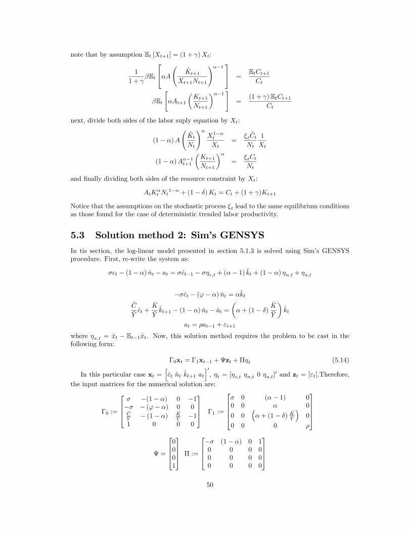
note that by assumption Et [Xt+1] = (1 + )Xt:
1
1 + �Et
24�A ~Kt+1
Xt+1Nt+1
!��1 35 =EtCt+1Ct
�Et
"�At+1
�Kt+1
Nt+1
���1 #=
(1 + )EtCt+1Ct
next, divide both sides of the labor suply equation by Xt:
(1� �)A ~Kt
Nt
!�X1��t
Xt=
�t ~CtNt
1
Xt
(1� �)A��1t+1
�Kt+1
Nt+1
��=
�tCtNt
and �nally dividing both sides of the resource constraint by Xt:
AtK�t Nt
1�� + (1� �)Kt = Ct + (1 + )Kt+1
Notice that the assumptions on the stochastic process �t lead to the same equilibrium conditionsas those found for the case of deterministic trended labor productivity.
5.3 Solution method 2: Sim�s GENSYS
In tis section, the log-linear model presented in section 5.1.3 is solved using Sim�s GENSYSprocedure. First, re-write the system as:
�ct � (1� �) nt � at = �ct�1 � ��c;t + (�� 1) kt + (1� �) �n;t + �a;t
��ct � ('� �) nt = �kt
�C�Yct +
�K�Ykt+1 � (1� �) nt � at =
��+ (1� �)
�K�Y
�kt
at = �at�1 + "t+1
where �x;t = xt � Et�1xt. Now, this solution method requires the problem to be cast in thefollowing form:
�0xt = �1xt�1 +zt +��t (5.14)
In this particular case xt =hct nt kt+1 at
i0, �t = [�c;t �n;t 0 �a;t]
0 and zt = ["t]:Therefore,
the input matrices for the numerical solution are:
�0 :=
2664� �(1� �) 0 �1�� � ('� �) 0 0�C�Y
� (1� �) �K�Y
�11 0 0 0
3775 �1 :=
26664� 0 (�� 1) 00 0 � 0
0 0��+ (1� �) �K
�Y
�0
0 0 0 �
37775
=
26640001
3775 � :=
2664�� (1� �) 0 10 0 0 00 0 0 00 0 0 0
377550

with this system at hand, one can proceed to implement Sim�s routine GENSYS (in Matlab)as described in Sims (2002), and then obtain a solution for the model in the form:
xt = �xt�1 +zt +1Xs�0
AMsBEtzt+s+1 (5.15)
which gives, as usual, a system of policy rules forhct nt kt+1 at
ias functions of the states.
Again, one can proceed to either obtain moments analytically using the output matrices orgenerate series to compute "empirical" moments.
5.4 Varieties of RBC models
� Habbit formation
� Capital adjustment costs
� Variable K utilization
� Campbell�s mechanism
� Hansen�s indivisible labor
5.4.1 Asset pricing models (Lucas, Shiller)
Single asset enviroment
A simpli�ed version of Lucas (1978) tree. Suppose that there is no production and agents �nanceconsumption with an exogenous stochastic endowment !t, capital gains from selling shares ofa single traded asset carried from previous period Pt (�t � �t�1) and exogenous stochasticdividends from ownership of shares dt�t�1. The planner�s problem is therefore:
maxE01Xt=0
�tU (Ct)
s:t:
Ct + Pt (�t � �t�1) � dt�t�1 + !t
The household choice variables at t are fCt; �tg while the states are f�t�1; dt; !tg : The F.O.Cfor this problem are:
Pt = �Et�U 0 (Ct+1)
U 0 (Ct)(dt+1 + Pt+1)
�Ct + Pt (�t � �t�1) = dt�t�1 + !t
so that for given sequences of f�t�1; dt; !tg ; a feasible allocation fCt; �tg and price system fPtgthat satis�es the FOC and TVC for the HH and clear markets will solve the planners problem.
51

Multi-asset enviroment.
Consider a simple extension of the above model in which households can hold shares from kdi¤erent risky assets and a riskless asset, B. The planners problem now becomes:
maxE01Xt=0
�tU (Ct)
s:t:
Ct +kXj=1
Pjt (�jt � �jt�1) +Bt �kXj=1
djt�jt�1 + (1 + rt)Bt�1 + !t
now the FOC for this problem are:
[Ct] : �tU 0 (Ct) = �t
[Bt] : �t = Et�t+1 (1 + rt+1)
and k (one for each jth asset) FOC of the form:
�tPjt = Et [�t+1 (Pjt+1 � djt+1)]
hence the k + 1 Euler equations are:
U 0 (Ct) = �Et [U 0 (Ct+1)] (1 + rt+1)
Pjt = �Et�U 0 (Ct+1) (Pjt+1 � djt+1)
U 0 (Ct)
�for j = 1; :::k
5.5 Calibration
A calibration exercise is best understood in an example. Consider the RBC model of section5.1.2. The parameters to be calibrated in this model are:
� : = capital�s share of output
� : = subjective discount factor
� : = RRA coe¢ cient
� : = technology serial correlation
�2" : = variance of "t
5.6 Estimation methods
5.6.1 Generalized method of moments (GMM)
The theory of RCB gives rise to equations like (5.11)-(5.13) with stochastic content, which canbe expressed as:
E [f (Zt; �0)] = 0 (5.16)
where Zt = [Ct Kt Nt At] and �0 = [�o o �o �] is a vector of true parameters. For instance,if the true parameters were known, the Euler equation in (5.11):
�Et
"�At+1K
��1t+1 Nt+1
1��
Ct+1
#=1 +
Ct
52
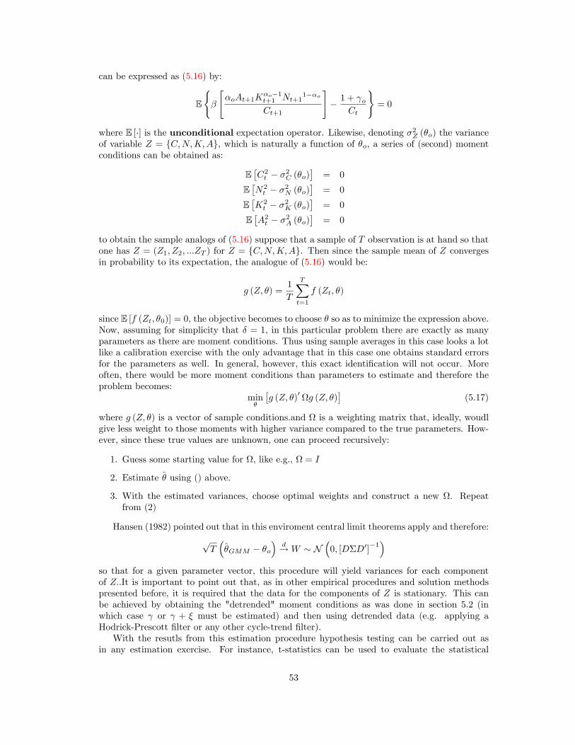
can be expressed as (5.16) by:
E
(�
"�oAt+1K
�o�1t+1 Nt+1
1��o
Ct+1
#� 1 + o
Ct
)= 0
where E [�] is the unconditional expectation operator. Likewise, denoting �2Z (�o) the varianceof variable Z = fC;N;K;Ag, which is naturally a function of �o, a series of (second) momentconditions can be obtained as:
E�C2t � �2C (�o)
�= 0
E�N2t � �2N (�o)
�= 0
E�K2t � �2K (�o)
�= 0
E�A2t � �2A (�o)
�= 0
to obtain the sample analogs of (5.16) suppose that a sample of T observation is at hand so thatone has Z = (Z1; Z2; :::ZT ) for Z = fC;N;K;Ag. Then since the sample mean of Z convergesin probability to its expectation, the analogue of (5.16) would be:
g (Z; �) =1
T
TXt=1
f (Zt; �)
since E [f (Zt; �0)] = 0, the objective becomes to choose � so as to minimize the expression above.Now, assuming for simplicity that � = 1, in this particular problem there are exactly as manyparameters as there are moment conditions. Thus using sample averages in this case looks a lotlike a calibration exercise with the only advantage that in this case one obtains standard errorsfor the parameters as well. In general, however, this exact identi�cation will not occur. Moreoften, there would be more moment conditions than parameters to estimate and therefore theproblem becomes:
min�
�g (Z; �)
0g (Z; �)
�(5.17)
where g (Z; �) is a vector of sample conditions.and is a weighting matrix that, ideally, woudlgive less weight to those moments with higher variance compared to the true parameters. How-ever, since these true values are unknown, one can proceed recursively:
1. Guess some starting value for , like e.g., = I
2. Estimate � using () above.
3. With the estimated variances, choose optimal weights and construct a new . Repeatfrom (2)
Hansen (1982) pointed out that in this enviroment central limit theorems apply and therefore:
pT��GMM � �o
�d!W � N
�0; [D�D0]
�1�
so that for a given parameter vector, this procedure will yield variances for each componentof Z:.It is important to point out that, as in other empirical procedures and solution methodspresented before, it is required that the data for the components of Z is stationary. This canbe achieved by obtaining the "detrended" moment conditions as was done in section 5.2 (inwhich case or + � must be estimated) and then using detrended data (e.g. applying aHodrick-Prescott �lter or any other cycle-trend �lter).With the resutls from this estimation procedure hypothesis testing can be carried out as
in any estimation exercise. For instance, t-statistics can be used to evaluate the statistical
53
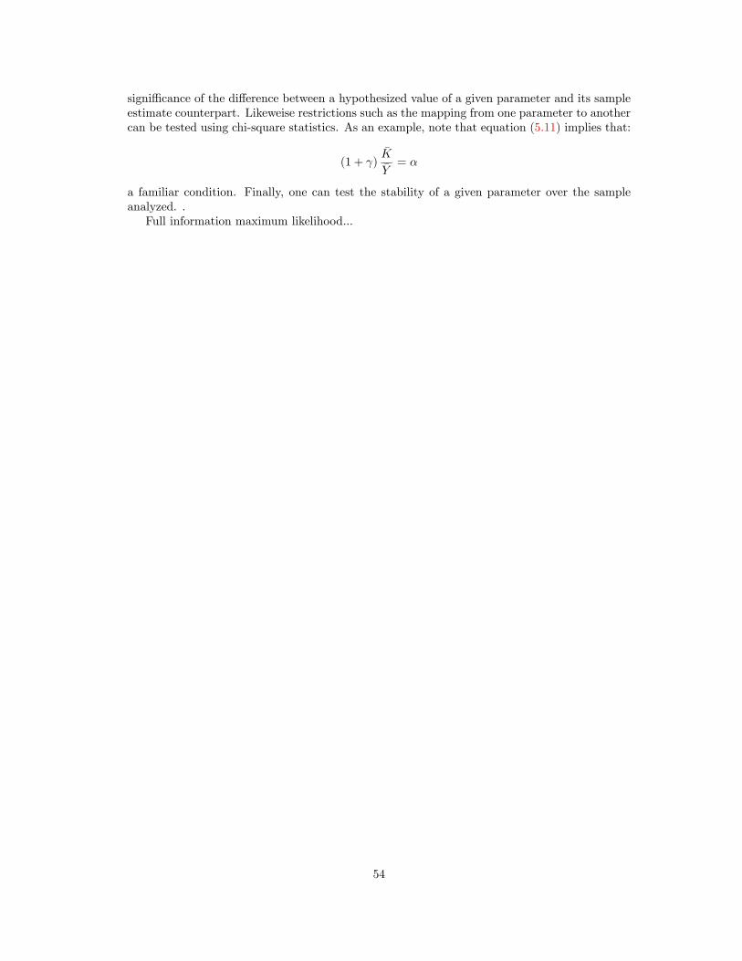
signi¢ cance of the di¤erence between a hypothesized value of a given parameter and its sampleestimate counterpart. Likeweise restrictions such as the mapping from one parameter to anothercan be tested using chi-square statistics. As an example, note that equation (5.11) implies that:
(1 + )�K�Y= �
a familiar condition. Finally, one can test the stability of a given parameter over the sampleanalyzed. .Full information maximum likelihood...
54

Bibliography
D. Acemoglu. Introduction to Modern Economic Growth. Princeton University Press, 2008.
C. Dave and D. De Jong. Structural Macroeconometrics. Princeton University Press, 2011.
A. Dixit. Optimization in Economic Theory. Oxford University Press, 1990.
A. Levy. Economic Dynamics: Applications of Di¤erence Equations, Di¤erential Equations andOptimal Control. Ashgate Publishing, 1992.
L. Ljungqvist and T. Sargent. Recursive Macroeconomic Theory. MIT Press, 2004.
D. Romer. Advanced Macroeconomics. McGraw-Hill, 2001.
N. Stokey and R. Lucas. Recursive Methods in Economic Dynamics. Harvard University Press,1989.
55

Part III
Appendixes
56

Appendix A
The dynamic programmingmethod
This appendix presents the various approaches to solving for the value function in a stationarydynamic programming problem along with an explicit derivation of the envelope condition.A typical dynamic programming problem includes:
� A state space S � Rm
� A control space A � Rn
� Instantaneous objective function: u : A� S ! R
� State transition function: g : A� S ! S
� Feasible control correspondence: � : S � A
� Discount factor: �
� Initial state: K0 2 S
Example 13 Suppose that S = A = R: Then the simplest "Cake-Eating" version of the Ramseyproblem is therefore:
max1Xt=0
�tpCt (A.1)
s:t:
g(Kt; Ct) = Kt � CtCt 2 [0;Kt]
K0 = �
so the Bellman Functional Equation for this problem is:
V (�) = maxC2[0;�]
hpC + �V (K � C)
i
57

A.1 Guess and verify
One method to solve the BFE is to try to guess the value function V (�). In order to come upwith a guess, solve the problem �rst as if it was a sigle-period maximization one:
maxpC
s:t: C 2 [0; �]
whose solution is:V0(�) =
p�
Next, guess that, for the multi-period problem, the solution to the BFE looks something like:
V (�) = ap� + b
where a; b are undetermined coe¢ cients. Now solve for a; b using the BFE:
V (� � C) =pC + �
hap� � C + b
iso that:
V (�) = ap� + b = max
C2[0;�]
npC + �
hap� � C + b
io(A.2)
at this point one can actually maximize the RHS since under the assumed value function. Todo so, di¤erentiate w.r.t. C and set equal to zero. Since the term inside the braces is a concavefunction, this would be in fact a maximizer. The result of this maximization is:
C =�
1 + (a�)2
replacing this maximizer in (A.2) one obtains:
ap� + b =
q1 + (a�)
2p� + �b
so that the undetermined coe¢ cients are:
a =
q1 + (a�)
2
a =1p1� �2
and:
�b = b
b = 0
so that �nally one is ready to verify the initial guess. To do so, one must show that:
1p1� �2
p� = max
C2[0;�]
hpC + �V (� � C)
i= V (�)
= maxC2[0;�]
"pC + �
p� � Cp1� �2
!#= V (�)
58
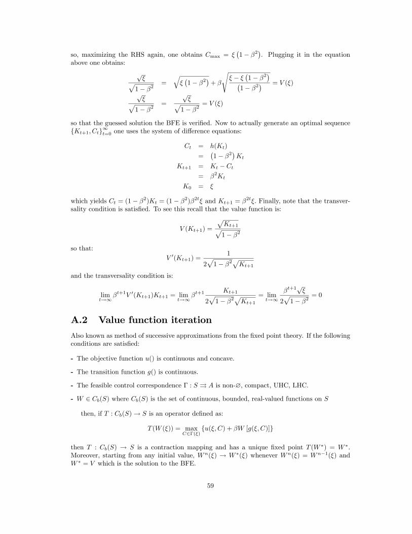
so, maximizing the RHS again, one obtains Cmax = ��1� �2
�. Plugging it in the equation
above one obtains:
p�p
1� �2=
q��1� �2
�+ �
s� � �
�1� �2
��1� �2
� = V (�)
p�p
1� �2=
p�p
1� �2= V (�)
so that the guessed solution the BFE is veri�ed. Now to actually generate an optimal sequencefKt+1; Ctg1t=0 one uses the system of di¤erence equations:
Ct = h(Kt)
=�1� �2
�Kt
Kt+1 = Kt � Ct= �2Kt
K0 = �
which yields Ct = (1� �2)Kt = (1� �2)�2t� and Kt+1 = �2t�: Finally, note that the transver-sality condition is satis�ed. To see this recall that the value function is:
V (Kt+1) =
pKt+1p1� �2
so that:V 0(Kt+1) =
1
2p1� �2
pKt+1
and the transversality condition is:
limt!1
�t+1V 0(Kt+1)Kt+1 = limt!1
�t+1Kt+1
2p1� �2
pKt+1
= limt!1
�t+1p�
2p1� �2
= 0
A.2 Value function iteration
Also known as method of successive approximations from the �xed point theory. If the followingconditions are satis�ed:
- The objective function u() is continuous and concave.
- The transition function g() is continuous.
- The feasible control correspondence � : S � A is non-?, compact, UHC, LHC.
- W 2 Cb(S) where Cb(S) is the set of continuous, bounded, real-valued functions on S
then, if T : Cb(S)! S is an operator de�ned as:
T (W (�)) = maxC2�(�)
fu(�; C) + �W [g(�; C)]g
then T : Cb(S) ! S is a contraction mapping and has a unique �xed point T (W �) = W �.Moreover, starting from any initial value, Wn(�) ! W �(�) whenever Wn(�) = Wn�1(�) andW � = V which is the solution to the BFE.
59
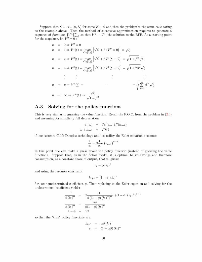
Suppose that S = A = [0;K] for some K > 0 and that the problem is the same cake-eatingas the example above. Then the method of successive approximation requires to generate asequence of functions fV ng1n=0 so that V n ! V �, the solution to the BFE. As a starting pointfor the sequence, let V 0 = 0 :
n = 0) V 0 = 0
n = 1) V 1(�) = maxC2[0;�]
hpC + �
�V 0 = 0
�i=p�
n = 2) V 2(�) = maxC2[0;�]
hpC + �V 1(� � C)
i=
q1 + �2
p�
n = 3) V 3(�) = maxC2[0;�]
hpC + �V 2(� � C)
i=
q1 + 2�2
p�
......
......
n = n) V n(�) = � � � =
s1Pn=1
�2tp�
n ! 1) V n(�)!p�p
1� �2
A.3 Solving for the policy functions
This is very similar to guessing the value function. Recall the F.O.C. from the problem in (2.4)and assuming for simplicity full depreciation:
u0(ct) = �u0(ct+1)f0(kt+1)
ct + kt+1 = f(kt)
if one assumes Cobb-Douglas technology and log-utility the Euler equation becomes:
1
ct= �
1
ct��kt+1
���1at this point one can make a guess about the policy function (instead of guessing the valuefunction). Suppose that, as in the Solow model, it is optimal to set savings and thereforeconsumption, as a constant share of output, that is, guess:
ct = � (kt)�
and using the resource constraint:
kt+1 = (1� �) (kt)�
for some undetermined coe¢ cient �: Then replacing in the Euler equation and solving for theundetermined coe¢ cient yields:
1
� (kt)� = �
1
� ((1� �) (kt)�)�� ((1� �) (kt)�)
��1
1
� (kt)� =
��
�(1� �) (kt)�
1� � = ��
so that the "true" policy functions are:
kt+1 = �� (kt)�
ct = (1� ��) (kt)�
60

which are of course, the same policy functions found in Example 2 of section 2.3 in the maintext.
A.4 Properties of the BFE
1. Claim 14 The mapping:
(T�) (x) = maxa2�(x)
fu (x; a) + �E� [f (x; a; ")]g (A.3)
is a contraction.
Proof (Blackwell conditions). First, to prove monotonicity: Let � (x) � ' (x) forevery x, then for every f(�) is continuous and � (x) closed-graph:
� [f (x; a; ")] � ' [f (x; �; ")]
maxa2�(x)
fu (x; a) + �� [f (x; a; ")]g � maxa2�(x)
fu (x; a) + �' [f (x; a; ")]g
moreover, since the operator E (�) preserves inequalities:
maxa2�(x)
fu (x; a) + �E� [f (x; a; ")]g � maxa2�(x)
fu (x; a) + �E' [f (x; a; ")]g
(T�) (x) � (T') (x)
so that T is a monotone operator. Next, to prove discounting: Let c 2 R, and note:
[T (�+ c)] (x) = maxa2�(x)
fu (x; a) + �E [� (f (x; a; ")) + c]g
= maxa2�(x)
fu (x; a) + �E�f (x; a; ") + �Ecg
= maxa2�(x)
fu (x; a) + �E�f (x; a; ")g+ �c
= (T�) (x) + �c
� (T�) (x) + c whenever � 2 [0; 1]
so that T (�) satis�es discounting. Therefore, T (�) satis�es both of Blackwell conditionsand thus is a contraction.
Claim 15 The operator T : D ! D in (A.3) maps the space of continuous, bounded,real-valued, increasing and concave functions into itself.
Proof. (step 0) Assumptions:
- For x 2 X, X is a convex subset of Rn
- � (�) is non-?-valued; convex-valued, compact-valued, U.H.C. and L.H.C.- For x0 > x00 ) � (x)
00 � � (x0)- u (�) is continuous, bounded, real-valued, increasing and concave on both arguments- f (�) is continuous, bounded in all its arguments- � (�) is bounded and continuous.- f (:; :; ") is an increasing mapping in x and concave in x; a.
- � 2 (0; 1)
61
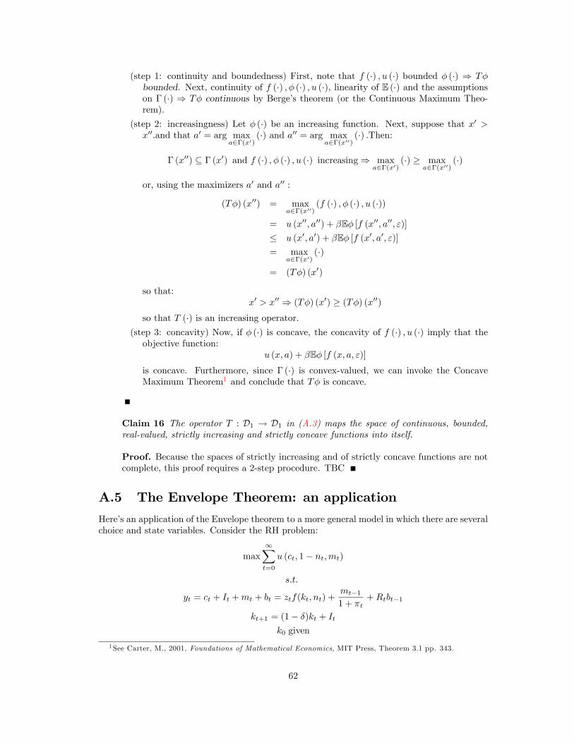
(step 1: continuity and boundedness) First, note that f (�) ; u (�) bounded � (�) ) T�bounded. Next, continuity of f (�) ; � (�) ; u (�), linearity of E (�) and the assumptionson � (�) ) T� continuous by Berge�s theorem (or the Continuous Maximum Theo-rem).
(step 2: increasingness) Let � (�) be an increasing function. Next, suppose that x0 >x00.and that a0 = arg max
a2�(x0)(�) and a00 = arg max
a2�(x00)(�) :Then:
� (x00) � � (x0) and f (�) ; � (�) ; u (�) increasing) maxa2�(x0)
(�) � maxa2�(x00)
(�)
or, using the maximizers a0 and a00 :
(T�) (x00) = maxa2�(x00)
(f (�) ; � (�) ; u (�))
= u (x00; a00) + �E� [f (x00; a00; ")]� u (x0; a0) + �E� [f (x0; a0; ")]= max
a2�(x0)(�)
= (T�) (x0)
so that:x0 > x00 ) (T�) (x0) � (T�) (x00)
so that T (�) is an increasing operator.(step 3: concavity) Now, if � (�) is concave, the concavity of f (�) ; u (�) imply that theobjective function:
u (x; a) + �E� [f (x; a; ")]
is concave. Furthermore, since � (�) is convex-valued, we can invoke the ConcaveMaximum Theorem1 and conclude that T� is concave.
Claim 16 The operator T : D1 ! D1 in (A.3) maps the space of continuous, bounded,real-valued, strictly increasing and strictly concave functions into itself.
Proof. Because the spaces of strictly increasing and of strictly concave functions are notcomplete, this proof requires a 2-step procedure. TBC
A.5 The Envelope Theorem: an application
Here�s an application of the Envelope theorem to a more general model in which there are severalchoice and state variables. Consider the RH problem:
max1Xt=0
u (ct; 1� nt;mt)
s:t:
yt = ct + It +mt + bt = ztf(kt; nt) +mt�11 + �t
+Rtbt�1
kt+1 = (1� �)kt + Itk0 given
1See Carter, M., 2001, Foundations of Mathematical Economics, MIT Press, Theorem 3.1 pp. 343.
62

where, as in a shopping time or MIU model, only cash provides direct utility. In this case, zt isa technology process with (for simplicity) deterministic constant growth:
zt = (1 + �) zt�1
and let at be the stock of �nancial assets at time t:
at =mt�11 + �t
+Rtbt�1
The state variables for this problem are fkt; bt�1;mt�1; ztg or simply fkt; at; ztg while the choicevariables are fct; nt; bt;mt; kt+1g. As usual, the BFE can be written as:
V (kt; at; zt) = maxct;nt;bt;mt
fu (ct; 1� nt;mt) + �V (kt+1; at+1; zt+1)g
s:t:
ct + kt+1 � (1� �)kt +mt + bt = ztf(kt; nt) +mt�11 + �t
+Rtbt�1
but bear in mind that:
V (kt+1; at+1; zt+1) = V
�ztf(kt; nt) +
mt�11 + �t
+Rtbt�1 + (1� �)kt �mt � bt � ct;mt
1 + �t+1+Rt+1bt; zt+1
�The F.O.C.s are:
[ct] : uc (ct; 1� nt;mt)� �Vk (kt+1; at+1; zt+1) = 0[nt] : un (ct; 1� nt;mt) + �Vk (kt+1; at+1; zt+1) ztfn(kt; nt) = 0
[mt] : um (ct; 1� nt;mt)� �Vk (kt+1; at+1; zt+1) + �Va (kt+1; at+1; zt+1)1
1 + �t+1= 0
[bt] : ��Vk (kt+1; at+1; zt+1) + �Va (kt+1; at+1; zt+1)Rt+1 = 0
Now, recall that, at the optimum (�) one will have policy functions for all the choice variables,so fc�t ; n�t ;m�
t ; b�t g are all functions of the state variables fkt; at; ztg : To save on notation, let
uj (ct; 1� nt;mt) = uj (t) and Va (kt+1; at+1; zt+1) = Va (t+ 1) : To derive explicitely the enve-lope condition totally di¤erentiate the value function:
Vk (kt; at; zt) =
�uc (t)
@c�
@kt+ un (t)
@n�
@kt+ um (t)
@m�
@kt
�+�
�Vk (t+ 1)
@k�t+1@kt
+ Va (t+ 1)@a�t+1@kt
�(A.4)
and note that a� depends on kt through m�t and b
�t , but the exogenous technology process zt
does not (i.e. @z@kt
= 0). Next, note:
k�t+1 = ztf(kt; n�t ) + (1� �)kt +
mt�11 + �t
+Rtbt�1 �m�t � b�t � c�t
so:@k�t+1@kt
= ztfk(kt; n�t ) + ztfn(kt; n
�t )@n�
@kt+ (1� �)� @c�
@kt� @m�
@kt� @b�
@kt(A.5)
while:
a�t+1 =m�t
1 + �t+1+Rt+1b
�t
so:@a�t+1@kt
=1
1 + �
@m�
@kt+Rt+1
@b�
@kt(A.6)
63

combining (A.6)-(A.5) into (A.4):
Vk (kt; at; zt) =
264 uc (t)@c�
@kt
+un (t)@n�
@kt
+um (t)@m�
@kt
375+�Vk (t+ 1)24 ztfk(kt; nt) + (1� �)ztfn(k
�t ; n
�t )@n�
@kt� @c�
@kt� @m�
@kt
�@b�
@kt
35+�Va (t+ 1)" 11+�t+1
@m�
@kt
+Rt+1@b�
@kt
#
rearranging:
Vk (kt; at; zt) = �Vk (t+ 1) (ztfk(kt; nt) + (1� �))+
8>>>><>>>>:@c�
@kt[uc (t)� �Vk (t+ 1)]+
+@n�
@kt[un (t)� �Vk (t+ 1) ztfn(k�t ; n�t ]
+@m�
@kt
hum (t)� �Vk (t+ 1) + �Va(t+1)
1+�t+1
i+@b�
@kt[�Va (t+ 1)Rt+1 � �Vk (t+ 1)]
9>>>>=>>>>;now, the F.O.C.s tell that each one of the terms in brackets is zero, so that the whole term inbraces vanishes:
Vk (kt; at; zt) = �Vk (t+ 1) [ztfk(kt; nt) + (1� �)]
but at the optimum (using the F.O.C.s again) uc (t) = �Vk (t+ 1) so replacing one �nally arrivesat the �rst envelope condition:
Vk (kt; at; zt) = uc (t) [ztfk(kt; nt) + (1� �)]
updating it one period and replacing in the F.O.C. for consumption, one arrives at the Eulerequation:
uc (ct; 1� nt;mt)
�uc (ct+1; 1� nt+1;mt+1)= [zt+1fk(kt+1; nt+1) + (1� �)] (A.7)
next, replacing on the F.O.C. for labor:
� un (ct; 1� nt;mt)
�uc (ct+1; 1� nt+1;mt+1)= [zt+1fk(kt+1; nt+1) + (1� �)] ztfn(kt; nt) (A.8)
but note that from the consumption Euler equation (A.7):
�uc (ct+1; 1� nt+1;mt+1) =uc (ct; 1� nt;mt)
[zt+1fk(kt+1; nt+1) + (1� �)]
so replacing in (A.8) one arrives at the intra-temporal Euler equation:
�un (ct; 1� nt;mt)
uc (ct; 1� nt;mt)= ztfn(kt; nt)
which, if one regards ztfn(kt; nt) as the real wage is a labor supply equation. Next, as a shortcutto the the second envelope condition, use the F.O.C. w.r.t bonds to obtain:
Va (kt+1; at+1; zt+1) =Vk (kt+1; at+1; zt+1)
Rt+1
so that using the �rst envelope condition:
Va (kt+1; at+1; zt+1) =uc (t+ 1) [zt+1fk(t+ 1) + (1� �)]
Rt+1
64
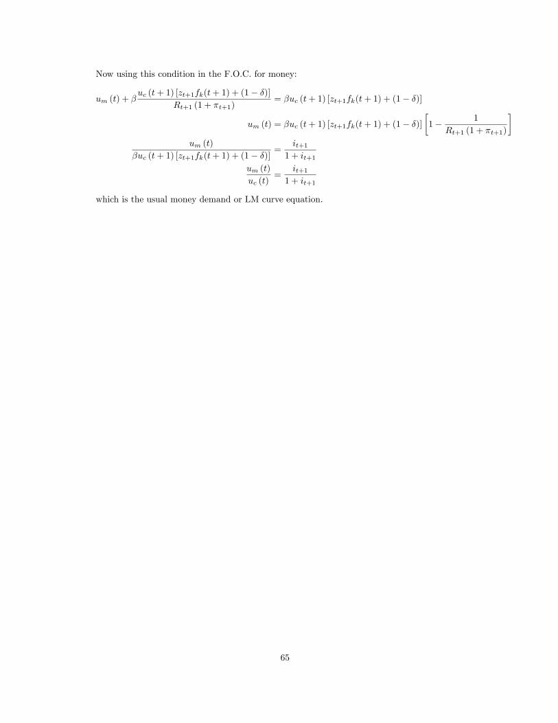
Now using this condition in the F.O.C. for money:
um (t) + �uc (t+ 1) [zt+1fk(t+ 1) + (1� �)]
Rt+1 (1 + �t+1)= �uc (t+ 1) [zt+1fk(t+ 1) + (1� �)]
um (t) = �uc (t+ 1) [zt+1fk(t+ 1) + (1� �)]�1� 1
Rt+1 (1 + �t+1)
�um (t)
�uc (t+ 1) [zt+1fk(t+ 1) + (1� �)]=
it+11 + it+1
um (t)
uc (t)=
it+11 + it+1
which is the usual money demand or LM curve equation.
65
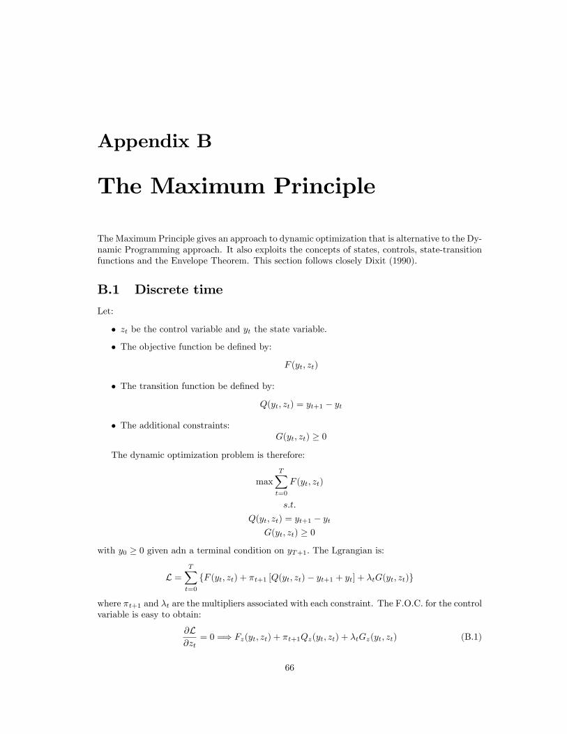
Appendix B
The Maximum Principle
The Maximum Principle gives an approach to dynamic optimization that is alternative to the Dy-namic Programming approach. It also exploits the concepts of states, controls, state-transitionfunctions and the Envelope Theorem. This section follows closely Dixit (1990).
B.1 Discrete time
Let:
� zt be the control variable and yt the state variable.
� The objective function be de�ned by:
F (yt; zt)
� The transition function be de�ned by:
Q(yt; zt) = yt+1 � yt
� The additional constraints:G(yt; zt) � 0
The dynamic optimization problem is therefore:
maxTXt=0
F (yt; zt)
s:t:
Q(yt; zt) = yt+1 � ytG(yt; zt) � 0
with y0 � 0 given adn a terminal condition on yT+1: The Lgrangian is:
L =TXt=0
fF (yt; zt) + �t+1 [Q(yt; zt)� yt+1 + yt] + �tG(yt; zt)g
where �t+1 and �t are the multipliers associated with each constraint. The F.O.C. for the controlvariable is easy to obtain:
@L@zt
= 0 =) Fz(yt; zt) + �t+1Qz(yt; zt) + �tGz(yt; zt) (B.1)
66
but the condition for the state variable is not so straightforward since each yt appears in twoterms of the in�nite sum. To circumvent this issue, re-write the relevant part of the Lagrangeanas:
TXt=0
�t+1 [yt � yt+1] = �1 [y0 � y1] + �2 [y1 � y2] + :::+ �T+1 [yT � yT+1]
= �1y0 � �1y1 + �2y1 � �2y2:::�T+1yT � �T+1yT+1
=TXt=1
yt (�t+1 � �t) + y0�1 � yT+1�T+1
so that the problem becomes:
L =TXt=1
[F (yt; zt) + �t+1Q(yt; zt) + yt(�t+1 � �t) + �tG(yt; zt)]
+ F (y0; z0) + �1Q(y0; z0) + y0�1 � yT+1�T+1)| {z }and note that the terms in braces pertain to t = 0; T + 1 whose values are given by initial andterminal conditions so no need to worry about them. From this formulation, it is clear why �t+1is given the name "co-state". Now, the F.O.C. for the state variable can be derived more easily:
@L@yt
= 0 =) �t+1 � �t + [Fy(yt; zt) + �t+1Qy(yt; zt) + �tGy(yt; zt)] = 0 8 t 6= 0; T + 1 (B.2)
This optimality condition states that, at the optimum, the overall marginal return from increas-ing yt is zero; that is, the shadow prices prevent pure or excess return from holding yt: Now,rearranging:
�t+1 � �t = � [Fy(yt; zt) + �t+1Qy(yt; zt) + �tGy(yt; zt)] (B.3)
next de�ne the Hamiltonian:
H(yt; zt; �t) = F (yt; z)t + �t+1Q(yt; zt) (B.4)
and note that the optimization problem does not consist simply in maximizing the instantaneousreward function F (�) since future reward depends upon future values of the state variable, whichin tunr is related to its current value and the choice variable via the state-transition functionQ(�): Next, de�ne the Lagrangian, L; for the single-period problem:
L = H(yt; zt; �t+1) + �tG(yt; zt) (B.5)
and here, H(yt; zt; �t) is the objective function of this single-period problem. Following F.O.C.(B.1), it is clear that zt is chosen so as to maximize (B.4), so let H(yt; z�t ; �t+1) = H�(yt; �t+1):Next, notice that:
@L
@yt= Fy(yt; zt) + �t+1Qy(yt; zt) + �tGy(yt; zt)
so we can replace this in (B.3):
�t+1 � �t = �@L
@yt= �Ly
But notice, in the static problem (B.5) the Envelope Theorem applies and thus Ly = H�y so:
�t+1 � �t = �H�y (yt; �t) (B.6)
67
and a similar envelope condition for the co-state variable gives L� = H��(yt; �t) = Q(yt; zt)
which replaced in the de�nition of the state-transition equation yields:
yt+1 � yt = H��(yt; �t) (B.7)
so the Maximum Principle states that �rst order necessary and su¢ cient conditions for theoptimization problem above are:
1. For each t, zt maximizes the Hamiltonian H(yt; zt; �t) subject to the single preiod con-straint(s) G(yt; zt):
2. The changes in yt; �t over time are governed by the pair of di¤erence equations (B.6)-(B.7).
B.2 Continuous time
State the problem above in continuous time:
max
TZ0
F (y(t); z(t))dt
s:t:
Q(y(t); z(t)) = _y(t)
G(y(t); z(t)) � 0
so that the (rearranged) Lagrangean is:
L =
TZ0
[F (y(t); z(t)) + �(t)Q(y(t); z(t)) + y(t)( _�(t)) + �(t)G(y(t); z(t))]
+ F (y(0); z(0)) + �1Q(y(0); z(0)) + y(0)�(0)� y(T )�(T )
The condition for zt to maximize the Hamiltonian is (assuming it is legitimate to di¤erentiateunder the integral sign):
@L@z(t)
= 0 =) Fz(y(t); z(t)) + �(t)Qz(y(t); z(t)) + �(t)Gz(y(t); z(t)) = 0
while the Hamiltonian itself is de�ned as:
H(y(t); z(t); �(t)) = F (y(t); z(t)) + �(t)Q(y(t); z(t))
and the pair of di¤erential equations (Pontryagin conditions) governing the behavior of the stateand co-state variables:
_y(t) = H��(y(t); �(t)) (B.8)
_�(t) = �H�y (y(t); �(t)) (B.9)
B.2.1 Current value vs. present value Hamiltonian
Using the notation above, suppose that:
F (y(t); z(t)) = e��tf(y(t); z(t))
68

so that the underlying objective function is the present-discounted value of the stream of instan-taneous utility functions f(y(t); z(t)): Then the present value hamiltonian above can be writtenas:
Hpv(y; z; �) = e��tf(y(t); z(t)) + �(t)Q(y(t); z(t))
Now suppose that it is desirable to state the problem in current value terms; the Hamiltonianwould be:
Hcv(y; z; �) = f(y(t); z(t)) + q(t)Q(y(t); z(t))
where:q(t) = �(t)e�t (B.10)
is the current-value shadow multiplier. Now revisit the Pontryagin conditions for the presentvalue problem:
@Hpv
@z(t)= 0 =) e��tfz(y(t); z(t)) + �(t)Qz(y(t); z(t)) = 0
_y(t) = Hpv� (y; z; �) = Q(y(t); z(t))
_�(t) = �Hpvy (y; z; �) = e��tfy(y(t); z(t)) + �(t)Qy(y(t); z(t))
Only the �rst and last of these conditions involve discounting so, rewrite the �rst in current-valueterms:
fz(y(t); z(t)) + �(t)e�tQz(y(t); z(t)) = 0
fz(y(t); z(t)) + q(t)Qz(y(t); z(t)) = 0 (B.11)
and rewrite the last condition, still in present-value terms as:
_�(t)e�t = fy(y(t); z(t)) + �(t)e�tQy(y(t); z(t)) (B.12)
now, since from (B.10):
_q(t) = _�(t)e�t + ��(t)e�t
= _�(t)e�t + �q(t)
_�(t)e�t = _q(t)� �q(t)
one can replace in (B.12) and:
_q(t)� �q(t) = fy(y(t); z(t)) + �(t)e�tQy(y(t); z(t))
_q(t)� �q(t) = fy(y(t); z(t)) + q(t)Qy(y(t); z(t)) (B.13)
is the Pontryagin condition for the costate variable corresponding to the current-value optimiza-tion problem.
69

Appendix C
First-Order Di¤erence Equationsand AR(1)
C.1 The AR(1) process
C.1.1 Representation and properties
Let "t � N(0; 1) iid shock. Then zt follows an AR(1) process if we can write it as:
zt = (1� ')� + 'zt�1 + �"tthis is the recursive formulation of the AR(1) process because it recurs in the same form at eacht. To go from the recursive formulation, to the in�nite order MA formulation, �rst replace zt�1in the expression for zt :
zt = (1� ')� + ' [(1� ')� + 'zt�2 + �"t�1] + �"tnext, repeat this recursive replacing and after k + 1 times one obtains:
zt = (1� ')�k�1Xj=0
'j + 'kzt�k + �
k�1Xj=0
'j"t�j
which can be rearranged as follows:
zt = �k�1Xj=0
'j � '�k�1Xj=0
'j + 'kzt�k + �k�1Xj=0
'j"t�j
= �
24'0 + k�1Xj=0
'j+1
35� '� k�1Xj=0
'j + 'kzt�k + �k�1Xj=0
'j"t�j
= � + �k�1Xj=0
'j+1 � �k�1Xj=0
'j+1 + 'kzt�k + �k�1Xj=0
'j"t�j
= � + 'kzt�k + �k�1Xj=0
'j"t�j
and if we let k !1 one gets:
zt = � + �1Xj=0
'j"t�j
70

that is, the in�nite-order MA representation of the AR(1) process, saying that the AR(1) processcan be written as an in�nite sum of past shocks. If j'j = 1 we have a unit root or say that zthas in�nite memory.
C.1.2 Conditional Distribution
The distribution of zt conditional on knowing zt�1: Recall that a linear function of a normal RVis itself a normal RV. Since at t the quantity zt�1 is known, it can be treated as a constant andtherefore zt, conditional on zt�1 is just a normal RV with its mean shifted by (1�')�+'zt�1:Toobtain the conditional mean and variance of zt �rst note that the variance remains unchangedas �2 while the mean:
Et�1 [zt] = Et�1 [(1� ')� + 'zt�1 + �"t]= Et�1 [(1� ')� + 'zt�1] + Et�1 [�"t]= (1� ')� + 'zt�1
so the conditional (on t� 1) distribution of zt :
zt �t�1 N((1� ')� + 'zt�1; �2)
C.1.3 Unconditional Distribution
The distribution of zt presuming no knowledge of zt�1; zt�2:::This is equivalent to the distrib-ution of zt conditional on knowing zt�k for a very large k, or, equivalently, the distribution ofzt+k for a very large k with information on t: This is why the unconditional distribution is alsocalled the long-run distribution. To obtain this, use the in�nite order MA representation:
Ezt = E
24� + � 1Xj=0
'j"t�j
35= � + E
24� 1Xj=0
'j"t�j
35= �
since j'j < 1 and each "t�j � N(0; 1). Likewise we could compute the unconditional mean as:
E [zt] = E [(1� ')� + 'zt�1 + �"t]= (1� ')� + 'E [zt�1]= (1� ')� + 'E [zt] (* E [zt] = E [zt�1])
so that solving:
(1� ')E [zt] = (1� ')�E [zt] = �
71

The unconditional variance is:
V ar [zt] = V ar
24� + � 1Xj=0
'j"t�j
35= V ar
24� 1Xj=0
'j"t�j
35=
0@�2 1Xj=0
'2j
1AV ar ["t�j ]
=�2
1� '2
note that in the last step the following expansion is used:
1Xj=0
'2j =
� 1'2�1 ('
1 � 1) if :' 2 f�1; 1g1 if ' 2 f�1; 1g
so that the unconditional distribution of zt is:
zt � N
��;
�2
1� '2
�Ntaurally, as long as 0 < j'j < 1 the unconditional variance is greater than the conditionalvariance.
C.2 Linear First-Order Di¤erence Equations (FODE)
Consider the linear FODE:xt � �xt�1 = b
can be solved using various techniques.
C.2.1 Induction & Geometric Series
Given an initian value x0:
x1 = �x0 + b
x2 = �x1 + b = �(�x0 + b) + b = �2x0 + �b+ b
x3 = �x2 + b = �(�(�x0 + b) + b) + b = �3x0 + �2b+ �b+ b
... =...
......
xt = �tx0 + �t�1b+ �t�2b+ :::+ �2b+ �b+ b
= �tx0 + bt�1Xk=0
�k
which using the geometric series arithmetic:
t�1Xk=0
�k =1� �t
1� �
72

we obtain:
xt = �tx0 + b
�1� �t
1� �
�so the solution to the LFODE takes the form:
xt = �t�x0 +
b
1� �
�+
b
1� �
C.2.2 Homogeneous part and General solution
An alternative 5-step approach is as follows:
1. Find the steady state of x (i.e., xt = xt�1 = �x):
�x =b
1� �
2. Find the solution to the homogeneous part :
xh;t � �xh;t�1 = 0 (C.1)
and let:xh;t = �t
be a solution to the homogeneous part for each t, so that:
xh;t�1 = �t�1
and (C.1) becomes:
�t � ��t�1 = 0
�t�1 (� � �) = 0
this equation has two solutions, the trivial solution where �t�1 = 0 and the non-trivialsolution (� � �) = 0 so using the latter:
� = �
and replacing in the hypothesized solution:
xh;t = �t
is the solution to the homogeneous part.
3. Find the General Solution: The general solution is a linear combination of the homogeneoussolution and the steady state:
xt =b
1� � + a�t
where a is the lin-comb undetermined coe¢ cient.
4. Find a for some initial x0 :
x0 =b
1� � + a�0 =) a = x0 �
b
1� �
5. Replacing in the general solution:
xt = �t�x0 �
b
1� �
�+
b
1� �which is, of course, the same result obtained by use of the induction technique.
73

C.2.3 Asymptotic Stability
The above solution can be expressed as:
f(x0) = �t�x0 �
b
1� �
�+
b
1� �
which has, as �xed point, x0 = b1�� , i.e.:
f
�b
1� �
�=
b
1� �
so b1�� can be interpreted as a stationary point ("steady-state"). We say that the above FODE
is asymptotically stable if:limt!1
(xt � �x) = 0
which will be the case only if:j�j < 1
and note that if 0 < � < 1 we observe a monotonic convergence towards �x while if �1 < � < 0the convergence is via oscilations around �x:
Example 17 A version of the Cagan (1956) model. Suppose that supply is based on expectedprices while demand is based on actual prices:
ydt+1 = �+ �pt+1
yst+1 = + �Etpt+1
and equilibrium is therefore given by:
�+ �pt+1 = + �Etpt+1
expectations are formed according to the adaptive behavior:
Etpt+1 � Et�1pt = �(pt � Et�1pt)
which can be written using the Lag operator as:
Etpt+1 = �pt + (1� �)LEtpt+1[1� (1� �)L]Etpt+1 = �pt
Etpt+1 =�pt
[1� (1� �)L]
nd replacing in the equilibrium condition:
�+ �pt+1 = + �
��pt
[1� (1� �)L]
���+ �pt+1 � �(1� �)pt = � + ��pt
pt+1 =�( � �)
�+
�1� �
�1� ��
��pt
74
and now we have a FODE without expectation terms which we can solve using the abovementioned
techniques. Using the 5 step method. Let �( ��)� = andh1� �
�1���
�i= then:
1) : Sty � Sate =) p� =
1�2) : Ph;t+1 = �t =) �t�1(� �) = 0
: =) ph;t+1 = t
3) : Gral:Sol: =) pt+1 =
1� + at
4) : Find coef =) p0 =
1� + a0
: =) a =
�p0 �
1�
�5) : Replace =) pt+1 =
1� +�p0 �
1�
�t
so that the solution to the price equation is:
pt+1 = � �1� � +
�p0 �
� �1� �
��1� �
�1� ��
��twith stationary price level equal to p� = ��
1�� and asymptotic stability condition:�����1� ��1� �������� < 1
C.3 Systems of linear FODE (or VDE)
Suppose that Xt is a 2-dimensional vector and:
Xt �MXt�1 = B
where M is a 2� 2 matrix known as the state-transition matrix and B is 2� 1:This system canbe solved in a similar fashion as single equations:
1. Solve for the steady state:�X = (I �M)�1B
2. Find the solution to the homogeneous part:
Xh;t �MXh;t�1 = 0 (C.2)
and again, suppose it has the shape:
Xh;t = A�t
so that:Xh;t = A�t�1
where A is a column vector of unknown parameters and � is some scalar. Replacing in(C.2) implies:
A�t �MA�t�1 = 0
�t�1A(�I �M) = 0
A(M � �I) = 0 (C.3)
75

Again, this equaton will have two solutions. However, we are only interested in the non-trivial solution so A 6= 0 which in turn implies that (M � �I) must be singular, i.e.:
det(M � �I) = 0
det
�m11 � � m12
m21 m22 � �
�= 0
which yields a quadratic equation in �:
�2 � (m11 +m22| {z })�+ (m11m22 �m12m21| {z }) = 0
�2 � tr(M) + det(M) = 0
the roots of this equation are called characteristic roots or eigenvalues. The two solutionsto this equation are:
�1; �2 =1
2
htr(M)�
ptr(M)2 � 4 det(M)
iand substituting �1; �2 in (C.3) results in the two eigenvectors of A :
A1 =
�1
m11��1m12
�and:
A2 =
�1
m11��2m12
�and the solution to the homogeneous system is given by the linear combination:
Xh;t = c1A1�t1 + c2A
2�t2
where c1; c2 are undetermined coe¢ cients.
3. Obtain the General Solution as in the previous section:
Xt = �X +Xh;t
Xt = (I �M)�1B + c1A1�t1 + c2A2�t2 (C.4)
4. As before, solve for the undetermined coe¢ cients using some initial value vector X0 :
X0 = (I �M)�1B + c1A1�01 + c2A2�02
this is a system of linear equations from which the coe¢ cients c1; c2 can be determined.Then substituting into (C.4) gives the solution to the VDE.
C.3.1 Asymptotic stability
It is easily seen that the asymptotic stability of the stationary point �X will depend upon theeigenvalues �1; �2 of the stae-transition matrix, A:Consider only the real-valued ones. If theyboth lie within the unit circle:
j�ij < 1 for i = 1; 2
the critical (stationary) point is asymptotically stable. If only one of them is inside the unitcircle, this implies that there are only two possible converging trajectories (i.e., a saddle-point).
76