Macroeconomics In The Macroeconomics In The Global EconomyGlobal Economy

Wei wei

Shool of Economics and Finance

Jiaotong University

Chapter 1 IntroductionChapter 1 Introduction

The approach of MacroeconomicsSome of the key questions addressed

by macroeconomicsMacroeconomics in historical

perspectiveProviding a broader framework for

macroeconomic analysis

The approach of The approach of MacroeconomicsMacroeconomics

What is macroeconomics ?

Macroeconomics is the study of aggregate behavior in an economy. While the economic life of a country depends on millions of individual actions taken by business firms, consumers, workers, and government officials, macroeconomics focuses on the overall consequences of these individual actions. For example, prices---- price index.

The approach of MacroeconomicsThe basic approach of Macroeconomics is

to look at the overall trends in the economy. Special summary measures of economic

activity ---GNP, the saving rate, or the consumer price index--- give the “big picture” of changes and trends.

These overall macroeconomic measures provide the basic equipment that allows macroeconomists to focus on the dominant changes in the economy.

How do economists do their job? First, try to understand on a theoretical

level the decision processes of individual firms and households.

Second, try to explain the overall behavior of the economy by aggregating, or adding up, all the decisions of the individual households and firms in the economy.

Third, giving empirical content to theory by collecting and analyzing actual macroeconomic data.

Some of the key questions Some of the key questions addressed by macroeconomicsaddressed by macroeconomics

The most important single measure of production in the economy is the GNP.

Economic growth and business cycles Unemployment is a second key variable that

macroeconomics investigates. A third key variable that interests

macroeconomists is the inflation rate. The fourth major variable that macroeconomists

look at is the trade balance.

Macroeconomics in historical Macroeconomics in historical perspectiveperspective

The creation of macroeconomics Economic statisticians began to collect and

systematize aggregate data which provided the scientific basis for macroeconomic investigations.

The careful identification of business cycle as a recurrent economic phenomenon.

The Great Depression A new theoretical framework to explain the

Great Depression proposed by Keynes.

The development of macroeconomics Keynesian and neo-Keynesian Main idea Keynes’s policy recommendation is the major t

ool of promoting economic growth. Non- Keynesian In fact, to many economists, it began to appear

that stabilization policies were actually a major source of renewed instability.

A “counterrevolution” began. Monetarism and it’s central idea. New classical macroeconomics: Lucas and Bar

ro. Advocates of the real business-cycle theory.

Providing a broader framework Providing a broader framework for macroeconomic analysisfor macroeconomic analysis

The general theory is limited to short-term economic fluctuations and stabilization policies.

Our analysis is pushed further by providing an especially broad view of macroeconomics.

Beside the attention on short-term economic fluctuations and stabilization policies, we focus more attention on other central concerns of macroeconomics,such as the determination of economic growth rate, or balance of payment, etc.

Considerable attention has been given to the differences in economic institutions in different countries in order that we discover a more general macroeconomic theory.

Chapter 2 Basic Concepts in Chapter 2 Basic Concepts in MacroeconomicsMacroeconomics

Looking at different measures of aggregate income and outcome and their interrelationship.

The process of aggregating across many different goods and services requires some common unit of measure: the role of price and price indexes.

A subject that permeates much of discussion in macroeconomics:Flows and Stocks

Two factors that influence the Intertemporal decisions of economic agents:Interest Rates and Present Value.

Another factor that is vital in understanding decision making across time periods: expectations

GDP and GNPGDP and GNP

What are GDP and GNP?How to calculate them? interrelationship of them GNP = GDP ＋ NFPGNP per capita and economic well-being

Real Versus Nominal VariablesReal Versus Nominal VariablesThe construction of price indexes Consumer price index or consumer price defl

ator

Pct = w1(P1t ／ P10) + w2(P2t ／ P20) + …+ WN(PNt ／ PN0)

Ct = nominal consumption expenditure ／ Pct

= Pct Ct ／ Pct

Deflator for investment spending (PI), government spending (PG), exports (PX), and imports (Pm)

Real GDP To calculate real production, we think of the GDP of the

economy as equal to the product of “average” price level in the economy, multiplied by the level of real production in the economy.

GDP = PQ

How to calculate Q ? We start with the definition of Nominal GDP as the sum

of final expenditures throughout the economy. Then, we use the price indexes for consumption,

investment, government spending, exports and imports to calculate a time series of real expenditures for each of these categories.

Finally, we can get Q by adding up the sum of final expenditures of these categories.

How can we get P ? Once getting real GDP, Q, then we can compute

the GDP price deflator P using the formula as follow:

P = GDP ／ Q

Generally, we get Real GDP by using the formula as follow:

Q = GDP ／ P

Flows and Stocks in MacroeconomyFlows and Stocks in Macroeconomy A flow is an economic magnitude measured as a

rate per unit of time. A stock is an economic magnitude measured at a

point of time. Investment and the capital stock Saving and wealth The current account and net international

investment position Deficit and the stock of public debt

Some Intertemporal Aspects of MacroecoSome Intertemporal Aspects of Macroeconomics: Interest Rates and Present Valuenomics: Interest Rates and Present Value

ss Many key macroeconomics issues involve choices

that not only take place in time but that involve decisions about timing. We call the choices involve later as intertemporal choice.

Two crucial elements in the analysis of intertemporal decisions

Interest rates and net present values Using interest rates, we can translate a given time

path of money in the future into a present value today. an economic magnitude measured

The Role of ExpectationThe Role of Expectation At the time that economic agents make intertemporal choices,

they are generally uncertain about the future, so they have to formulate some expectations about the future.

How do economic agents actually formulate their expectations ?

Static expectations Next year is going to be like this year. Adaptive expectations Individuals update their expectations about future dependin

g on the extent to which their expectations about present period turned out to be wrong.

Rational expectation Individuals make efficient use of all available information. What economic model the individuals is using and just wha

t economic information he or she has at hand.

Chapter 3 Output Determination: Chapter 3 Output Determination: Introducing Aggregate Supply and Introducing Aggregate Supply and

Aggregate DemandAggregate Demand

Macroeconomics as the study of economic fluctuations

The Determination of aggregate supply The classical approach to aggregate supply The Keynesian approach to aggregate supply The determination of aggregate demand Equilibrium of aggregate supply and aggregate

demand Aggregate supply and demand in the short run and

the long run

Macroeconomics as the study Macroeconomics as the study of economic fluctuationsof economic fluctuations

Economic fluctuations have been a central concern of macroeconomics

Economic fluctuations: output and employment fluctuations

Unemployment rate Potential output, current output and output gap When employment fluctuates, so does output, since output is

produced using labor inputs. Just as we measure the extent to which employment falls short of the full-employment level, we also can measure the extent to which output falls short of the level that would be produced if all labor were fully employed.

Economic performance is not only measured in terms of the general trend of output, but also in terms of whether the output gap is increasing or decreasing.

Okun’s law There is a great regularity that a reduction of unemploy

ment of 1 percent of labor force in the US was associated with a rise in GNP and fall in the output gap of 3 percent.

Business cycle Unlike periods of sustained unemployment, business cy

cles represent shorter-term fluctuations of output and employment, typically lasting 3-4 years.

A key feature of business cycles is that important macroeconomic variables-output, prices, investment, business profits, and various monetary variables-tend to move together in a systematic fashion.

The Determination of aggregate The Determination of aggregate supplysupply

Aggregate supply Definition Aggregate supply is the total amount of output

that firms and households choose to provide, given the pattern of wages and prices in the economy.

Optimal supply decision In fact, supply decision bases not only on

current wages and prices, but also on expectations about future wages and prices.

Formulation of aggregate supply The Formulation of aggregate supply is

complicated by the fact that there are many kinds of goods in the economy, produced by a very large number of firms and households.

Our theoretical framework ignores these complications and assumes that the economy produces a single output.

The production Function Q ＝ Q (K, L, τ) In the equation, output is a function of the capital

and labor used in production and of the state of technology.

The production function has two characteristics: An increase in the amount of any input will

make output go up. We assume that the marginal productivity of

each factor declines as more of that factor is used with a fixed amount of the other factor.

BQ=(K0,L)

Q

L

Q

Q(K1 ＞ K0)

Q(K1)

L

MPL

LMPL(K0)

MPL(K1 ＞ K0)

(a) Production function (b) Marginal productivity of labor

The demand for labor and the output supply function

The firm should hire labor until the marginal product of labor input equals the real wage.

w/p, MPL

(w/p)a

(w/p)b

La Lb

L

We can summarize these findings by writing the demand for labor as a function of real wage and the levels of capital and technology:

LD = LD(w/P, K, τ ) Using the labor-demand schedule. We can

now derive an output supply schedule which shows the amount of output the profit-maximizing firm will supply at each level of w/p, K, and τ.

QS = QS ［ LD(w/P, K, τ ) ， K, τ ］ Note that QS is a negative function of w/p for

an “indirect” reason.

Note also that QS is a positive function of K and τ,for direct and indirect reasons.

More simply, output supply is a negative function of w/p and a positive function of K and τ:

QS = QS (w/P, K, τ )The Supply of Labor The supply schedule for labor, LS

Labor-supply decision: Household must choose between supplying labor and enjoying leisure, the so-called Labor-leisure decision.

Assumptions A worker must choose only between lab

or and leisure and in which he consumes all his wage earnings,which are his only source of income.

The worker can choose to work any number of hours per day.

UL = UL(C, L)

C

L

UL2 UL1

UL0

△L

△C0

△L

△C1 > △C0

A

B

How much labor and consumption workers actually choose depends both on the utility function and on the real wage level.

C0 = (w/p) 0

C1 =3 (w/p) 0

C

L

Z1[(w/p) 1> (w/p) 0 ]

Z0[ (w/p) 0 ]

1 2 3

C

L

UL2

UL1

Z1[(w/p) 1 ]

Z2[(w/p) 2 ]

C2

C1

(w/p)

L

(w/p) 1

(w/p) 2

L 1 L 2

Substitution effect and Income effect Substitution effect means that each hour of leisure

represents a greater amount of forgone consumption of goods when the real wage goes up. With leisure more expensive, households “substitute” away from it and choose longer working hours.

Income effect works to reduce labor supply when wages increase.

The effect of a rise in wages on the supply of labor is theoretically ambiguous: the substitution effect tends to increase L, the income effect tends to decrease L. The relative influence of these two effects depends on household preferences.

The Classical Approach to The Classical Approach to Aggregate SupplyAggregate Supply

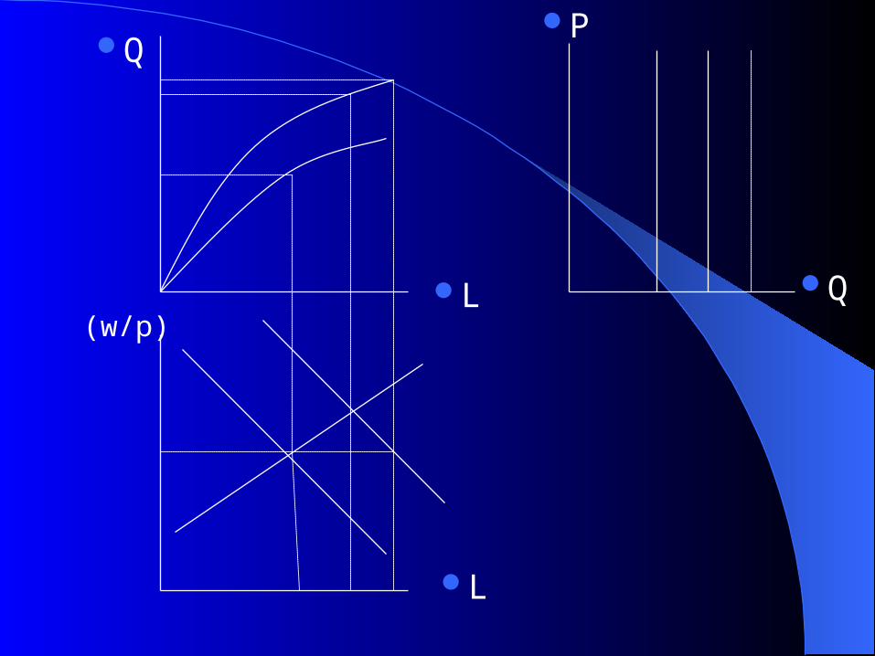
We already derived the Aggregate supply function, the demand for labor, and the supply of labor. Now we combine these and summarize the results in an aggregate supply curve.

The Main idea of classical approach For any price level, the nominal wage is fully

flexible and adjusts to keep the supply of labor and the demand for labor equilibrated. Thus, the real wage is determined so as to clear the labor market.

Q

L

Qf

Q(K0, L)

(w/p)

LLf

LD

LS

P

Q

QS

Deriving the aggregate supply curve How does the supply of aggregate output

respond when the price level increase?

Q

L(w/p)

L

P

Q

Unemployment in the classical approach Amendments to the basic model One amendment allows for the fact that

some people may choose voluntarily to be unemployed, at least for short periods of time.

A second amendment emphasizes that various forces in the labor market-- laws, institutions, traditions-- may prevent the real wage from moving to its full-employment level. If the real wage is stuck above the full-employment level, the unemployment results.

The Keynesian approach to aggregate supply Assumption: Nominal wages and prices do n

ot adjust quickly to maintain labor-market equilibrium.

Sticky wages Long-term labor contracts As the price level(P) rises, the real wage fal

ls, the desired level of labor input goes up, the desired level of output supply also rises. As a result, the aggregate supply curve is upward sloping.

Involuntary unemployment Involuntary unemployment is that some people

who are willing to work at the wage received by other workers of comparable ability cannot do so.

Why does involuntary unemployment arise? Nominal wage rigidity(Keynesian) Real wage rigidity(classical theory)Aggregate Supply: a summary classical aggregate supply Keynesian aggregate supply extreme Keynesian aggregate supply

Qs Qs

Qs

P

Q Q Q

The determination of aggregate demand The equilibrium level of output and the price level

over an entire economy is determined by the interaction of aggregate supply and aggregate demand.

The structure of aggregate demand with a closed economy

QD = C + I + G Aggregate demand curve Real Balance Effect One immediate effect of a price increase is to

reduce the real value of money held by the public.

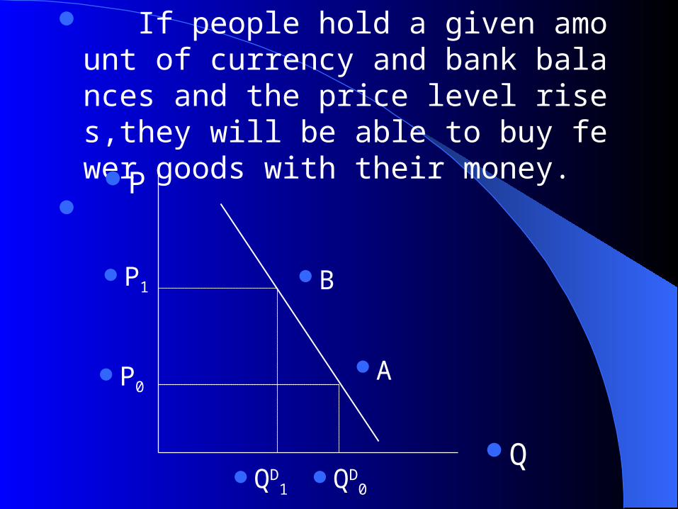
If people hold a given amount of currency and bank balances and the price level rises,they will be able to buy fewer goods with their money.

P

Q

B

A

P1

P0

QD1

QD0

In an open economy, aggregate demand is the total amount of domestic goods demanded at the given level of prices by both domestic and foreign purchasers.

The aggregate demand schedule in the open economy is still down-word-slope.

In the open economy, as in the closed economy, a rise in the price level tends to cause a fall in aggregate demand.

A rise in domestic prices compared with foreign prices makes it more expensive to buy domestic goods and relatively less expensive to buy foreign goods.

The Equilibrium of Aggregate Supply And Aggregate Demand

The aggregate supply-aggregate demand framework is useful apparatus for determining the equilibrium of output and the price level. We can use this framework to study the effects of specific economic policies as well as of external shocks on the equilibrium levels of Q and P.

Output market equilibrium is given by the intersection of the aggregate demand curve and aggregate supply schedule. This equilibrium will also determine the level of employment in the economy.

Equilibrated level of output does not signify the optimal level of output. There might by output gap.

Change on equilibrium: Demand side Aggregate demand expansion Changes in monetary, fiscal, and exchange-rate

policies shift the position of aggregate demand schedule.

Expansionary monetary, and fiscal policies and devaluated exchange-rate policy can result in aggregate demand expansion

P

A demand expansion in the classical case

Q

QS

QD’

QD

P1

P

0

Qo

A demand expansion in the Keynesian case

P

Q

QD’

QD

P

1P

0

QS

Q

o

Q1

A demand expansion in the Keynesian extremeA demand expansion in the Keynesian extreme case case

P

Q

QD’

QD

P QS

Q

o

Q1

-

Under classical conditions, a rise in aggregate demand leads only to a rise in prices, with no effect on output.

In the keynesian case, an aggregate demand expansion raises output (and employment) as well as the price level. It leads to the important conclusion that policy changes can, in the keynesian case, affect output.

Change on equilibrium: supply side A supply shock: once-and-for-all technol

ogical improvement

A technological improvement in the Classical case

P

Q

QD

P

0

QS0

Q

o

Q1

QS1

P

1

A technological improvement in the basic Classical case

P

Q

QD

P

0

QS0

Q

o

Q1

QS1

P

1

A technological improvement in the extreme Classical case

P

Q

QD

P0=w/a0QS

0

Q

o

Q1

QS1

P1=w/a1

Source of economic fluctuation Macroeconomists differ about the shape of the aggr

egate supply schedule. Macroeconomists differ about the relative importanc

e of the different kinds of shocks that hit an economy.

Aggregate Supply And Demand In The Short Run And The Long Run

Keynes stressed nominal wages do not necessarily adjust instantly to maintain full employment. But Keynes himself, and later economists working in his tradition, recognized nominal wages are not truly fixed; they simply adjust slowly to imbalances of aggregate demand.

Dynamic equation for wages ^ W+1

= (W+1

– W)/ W

^

W+1 = a(Q – Q

f )

Short- and long-term Effects of an aggregate dem

and Contraction

P

Q

QD

QD’

P

0P

1

QS

QS’E

A

E’P2

Q1Q

f

Short-term Effects of an aggregate demand Contraction

Aggregate demand declines, the immediat

e result is to shift output from Qf at point E

down to Q1 at point A.

long-term Effects of an aggregate demand

ContractionWith the reduction of output, nominal wage

s tend to fall. And as nominal wages fall, the aggregate supply curve shift to the right

After the full adjustment of nominal wages,output is back to the full-employment level, and the full effect of the shock to aggregate demand appears as lower prices rather than lower output.

Economy shows Keynesian properties in the short run and classical properties in the long run. In this sense, the debate between modern Keynesian and modern classical economists is mainly about timing.

Chapter 4 Consumption and Chapter 4 Consumption and SavingSaving

Central issue: How households divide their income between consumption and saving.

Major topics: National Consumption and Saving The Basic Unit: The Household The Intertemporal Budget Constrain Household Decision Making The permanent-Income Theory of Consumption

The Life-Cycle Model of Consumption and Saving

Household Liquidity Constrains and Consumption Theory

Aggregate Consumption and National Saving Rates

Consumption, Saving and the Interest Rate Business Saving and Household Saving:

Theory and Evidence

The Framework of analysis: The Cumulative effect of the consumption and sa

ving decisions of households helps to determine the rate of growth of the economy, the trade balance, and the level of output and employment.

The analysis of consumption and saving decision relies heavily on a life-cycle theory of consumption and saving

Keynes’ consumption theory Our strategy in understanding total saving in the ec

onomy is to start with the household, then add firm behavior, and finally add government saving behavior

National Consumption and SavingNational Consumption and SavingAs we construct the theory of household

saving and consumption, we focus on the choice of consuming or saving out of disposable personal income.

How to calculate the disposable personal income?

Personal saving, gross business saving, and government saving

The compare of gross saving rate among different countries

The Basic Unit: The householdThe Basic Unit: The householdMuch data are collected on level of househo

ld, rather than on the level of the individuals that compose the family.

Assumption: Nonmonetary economy and numeraire g

oods A given household produces a stream of

output Q1, Q2, ...Qt over T periods and consumes an amount C1, C2, …Ct .

If the household lives in isolation, and if the output is not storable, then the household has to consume each period exactly what it produces or let some of its output go to waste.

if the output is storable, the household might be able to store some of the output in some periods and the consume out of this accumulated savings in other periods.

Even if the output is not storable, the household still can save if the household is linked to other households through a market for financial assets.

The existence of financial assets greatly enhances the possibilities open to households to adjust their profiles of consumption over time for any given time path of output.

Income and output Y = Q + r B-1

Stock of bonds B = B-1 + ( Y - C) = B-1 + (Q + r B-1 - C)

Saving in the period B - B-1 = S

The Intertemporal Budget ConstraintThe Intertemporal Budget ConstraintThe budget constraint in the two-period model Assumptions Households inherit no assets from the past

and finish their life with no assets ether. B0 = 0 B2 = 0

B1 - B0 = B1 = S1

B2 - B1 = S2

- B1 = S2

Conclusion The decision for households is not

whether to save or whether to borrow, but rather when to save and when to borrow.

S1 = Y1 - C1 = Q1 - C1 = B1

S2 = Y2 - C2 = Q2 + r B1 - C1

C1 + C2/(1 + r) = Q1 + Q2 /(1 + r) = W1

Receive an inheritance C1 + C2/(1 + r) = (1+ r) B0 + Q1 + Q2 /(1 + r)

Period 2

Period 1

A

B

QQ2

Q1

Household Decision MakingHousehold Decision MakingThe intertemporal utility function UL(C1, C2)

The budget constraint of household

A

Period 2

Period 1

For a given level of current income, consumption depends not only on current income but also on future income. It also depends on interest rate and tastes of households

The Permanent-Income Theory of The Permanent-Income Theory of ConsumptionConsumption

Friedman: This year's consumption should depend on an average level of income expected this year and in future years.

Households tend to smooth consumption over time. Because income is bound to fluctuate year to year, households use capital markets to maintain fairly steady consumption against a backdrop of fluctuating income.

Permanent-income is defined as a kind of average of present and future incomes.

YP + YP/(1 + r) = Q1 + Q2 /(1 + r)

YP = (1 + r)/(2 + r)[Q1 + Q2 /(1 + r)]

S1 = Q1 - C1 = Q1 - YP

The special case of equal consumption each period holds only for particular kinds utility functions, but nonetheless, the ideas behind this case have more general validity. Households decide their consumption levels on the basis of their permanent income.

Three prototypical kinds of shocks to income Temporal current shocks Permanent shocks Anticipated future shocks The estimation of future income Adapted expectations

YP = aYP-1 + (1 - a)Y

Rational expectationEmpirical evidence on the permanent-inco

me modelDurables and nondurables The permanent-income hypothesis applies to co

nsumption, and consumption is not exactly the same thing as the expenditure on consumer goods.

Consumption is properly measured as the sum of expenditures on nondurables plus the flow of services rendered by the existing stock of consumer durables.

Consumption and taxes

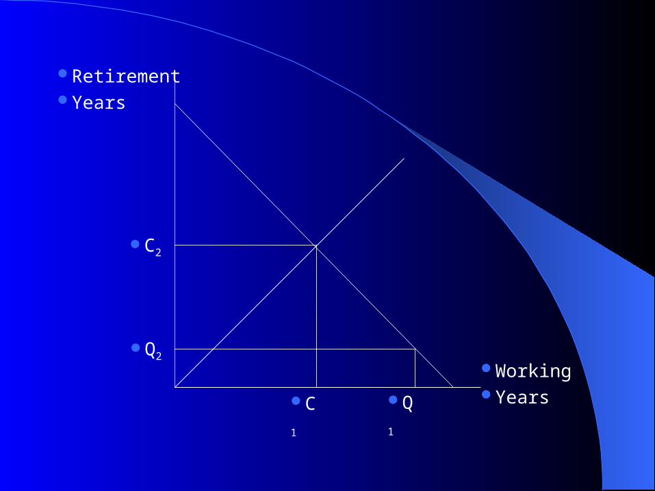
The Life-Cycle Model of The Life-Cycle Model of Consumption AND SavingConsumption AND Saving

The life-cycle model builds on the theory that consumption in a particular period depends on expectations about life-time income and not on the income of current period.

The distinctive contribution of the life-cycle hypothesis is its observation that income tends to fluctuate systematically over the course of person’s life and that personal saving behavior is therefore crucially determined by one’s stage in the life cycle.

Y,C

Time

+S

-S

Retirement Years

Working YearsC

1

C2

Q

1

Q2

Consumption during retirement is financed both from savings accumulated during the working years and from transfers that old people receive from the government and from their children.

Social security taxes and social security system. Some other implications of the life-cycle theory YP = (1 + r)/(2 + r)[Q1 + Q2 /(1 + r)] = k(r)W1

Consumption is a fraction of wealth, with the factor of proportionality (k), or the marginal propensity to consume out of wealth,depending on the interest rate, time preference and the ages of individuals in the household.

Evidence on the life-cycle model The role of bequests: What motivates bequests?

Household Liquidity Constraints and Household Liquidity Constraints and Consumption theoryConsumption theory

Households that cannot borrow and that lack a stock of financial wealth are said to be “liquidity constrained”, in that the most they can spend is the income that they earn in the current period.

Intertemporal theories of consumption are explicitly based on the assumption that agents can freely borrow and lend within the limits of their lifetime budget constraint.

Financial markets normally lend against collateral, not just the promise of future earnings from labor.

The proportion of liquidity constrained households is higher among young households than old ones.

Aggregate Consumption and National Aggregate Consumption and National Saving RatesSaving Rates

Macroeconomics foundations for macroeconomic variables.

Aggregating from the individual household to the whole economy

Simple case Complicated case: The aggregate saving in the economy is determined

by the balance of saving and dissaving, averaged over the entire population.

Model with “overlapping generations”

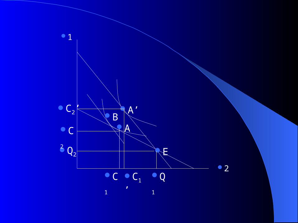
Consumption, Saving and Interest RateConsumption, Saving and Interest Rate

It is often supposed, somewhat naively, that as interest rates rise, and thus, as the rate of return to saving increases, it must be the case that saving will also increase.

It is useful to divide the effect of the interest-rate increase into two parts: a “substitution effect,” which always tends to raise saving, and an “income effect,” which may raise or lower saving.

2

1

BA’

EA

C1C1’

C2

C2’

Q1

Q2

1

2

E

A’BA

Q

1

C1

’

C

1

Q2

C

2

C2’

Business Saving and Household Saving: Business Saving and Household Saving: Theory and EvidenceTheory and Evidence

Business firms are ultimately owned by households, and therefore the overall level of private saving is still basically determined by household behavior, and the division of saving between households and firms is somewhat arbitrary.