International Journal of Fracture 69: 201-228, 199411995. © 1995 Kluwer Academic Publishers. Printed in the Netherlands.

Macroscopic fracture characteristics of random particle systems

MILAN JIRASEK and ZDENEK P. BAZANT* Northwestern University, Evanston, Illinois 60208, USA

Received 3 January 1994; accepted in revised form 3 August 1994

201

Abstract This paper deals with detennination of macroscopic fracture characteristics of random panicle systems. which represents a fundamental but little explored problem of micromechanics of quasibrittle materials. The panicle locations are randomly generated and the mechanical properties are characterized by a triangular softening force­displacement diagram for the interparticle links. An efficient algorithm. which is used to repetitively solve large systems, is developed. This algorithm is based on the replacement of stiffness changes by inelastic forces applied as extemalloads. It makes it possible to calculate the exact displacement increments in each step without iterations and using only the elastic stiffness matrix. The size effect method is used to detennine the dependence of the mean macroscopic fracture energy and the mean effective process zone size of two-dimensional panicle systems on the basic microscopic characteristics such as the microscopic fracture energy, the dominant inhomogeneity spacing (particle size) and the coefficients of variation of the microstrength and the microductility. Some general trends are revealed and discussed.

1. Introduction

Fracture of quasi brittle materials, which is characterized by large zones of distributed cracking, can be effectively modeled by a particle system equivalent to a lattice with breaking links. Mechanical analysis of large systems of particles was initiated by Cundall [1], Serrano and Rodriguez-Ortiz [2], Rodriguez-Ortiz [3] and Kawai [4] who dealt with rigid particles that interact by friction and simulate the behavior of granular solids such as sand. This approach was developed and extensively applied by Cundall [5] and Cundall and Stack [6], who called it the distinct element method. An extension of Cundall's method to the study of microstructure and crack growth in geomaterials with finite interfacial tensile strength was introduced by Zubelewicz [7,8], Zubelewicz and Mr6z [9], and Plesha and Aifantis [10]. As demonstrated by Zubelewicz and BaZant [11], a particle model simulating the microstructure of an aggregate composite such as concrete can describe progressive distributed microcracking with gradual softening and with a large cracking zone. This model was modified and refined by BaZant et al. [12], who used it to study the size effect on the nominal strength and on the post-peak slope of load-deflection diagrams. They showed that the spread of cracking and its localization can be simulated realistically. Observing that it would hardly be possible to determine the macro-fracture energy by summing up the energies dissipated by fractured interparticle links, they showed that this is possible by using the size effect method. The particles were assumed to be elastic and have only axial interactions as in a truss. The interparticle contact layers of the matrix were described by a softening stress-strain relation.

• Walter P. Murphy Professor of Civil Engineering and Materials Science.

202 M. lirtisek and ZP. Bazant

The particle models are closely related to lattice methods, developed by theoretical physi­cists for the simulation of fracture processes in disordered materials (Charmet, Roux and Guyon [13], Herrmann [14], Herrmann and Roux [15]).

Van Mier and Schlangen recently developed a lattice model for fracture of concrete. They used regular (Schlangen and van Mier [16], van Mier and Schlangen [17)) as well as randomized (Schlangen [18], Schlangen and van Mier [19)) frameworks and a linear stress-strain law with a sudden stress drop and random strength to simulate a number of experiments.

The objective of this paper is to study the relationship of macroscopic fracture properties to microscopic characteristics of interparticle links and formulate an efficient numerical method for this purpose. Our approach will be based on the size effect method (BaZant [20], BaZant and Pfeiffer [21)), which has already been used for determining the macroscopic fracture energy of particle systems by BaZant et al. [12]. We will extend the size effect method to the determination of the effective fracture process zone size of particle systems and will study the effect of link characteristics and microstrength randomness on the macrofracture properties. We will also formulate a more efficient numerical method than that used before, permitting repeated analysis of large particle systems. This is especially important for the size effect method, for which very large particle systems must be solved.

Because of computer power limitations, the numerical simulation will be limited to two­dimensional particle systems. This is no doubt adequate for the simulation of fracture of sea ice plate on the scale of over 100 m or other problems of thin plates, but might not be very realistic for thick bodies.

2. Basic characteristics of particle systems

The relationship between the microscopic link properties, which enter the simulation as chosen parameters, and the macroscopic properties, which are observable on the scale of the structure, must be well understood before one can try to effectively control the behavior of the model and tune it up so that practical problems can be solved. The basic two macroscopic material characteristics governing the behavior of quasibrittle structures are the fracture energy and the effective length ofthe fracture process zone. One aim of this paper is to study their relationship to microstructure.

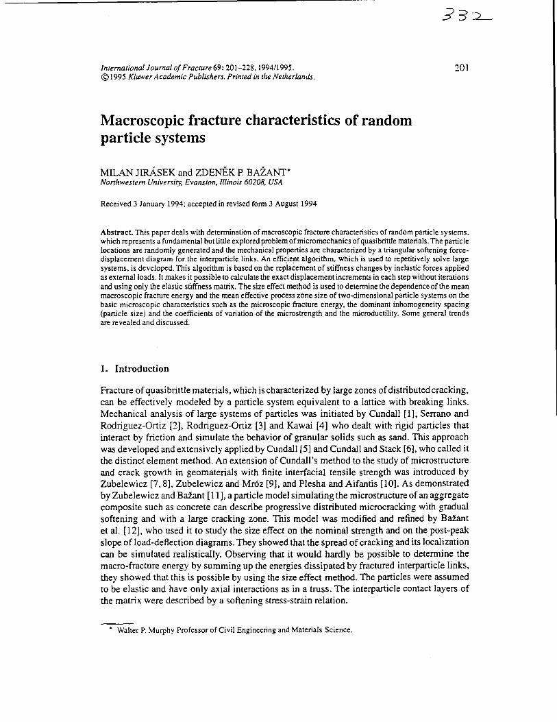
On the microscopic level, the" parameter having the strongest influence on the overall ductility is no doubt the fracture energy of the particle links. It is determined bithe strength it of the links, called the microstrength, and their microductility characterized by the ratio II = EIIEp, where Ep is the microstrain at peak microstress and EI is the microstrain at complete fracture (see Fig. la). A perfectly microbrittle model with a sudden drop of stress after the peak is characterized by I I = 1; a larger value of I I indicates an increase of microductility. The limit I I = 00 corresponds to ideal elastoplasticity.

Instead of the microductility one could use as the basic parameter the microfracture energy Gj, which represents the area under the interparticle stress-displacement curve. The assump­tion of constant Gj rather than constant I I is appropriate if there is one and only one crack within the length of each link, while the assumption of constant I I is appropriate if the number of cracks within the length of the link is proportional to L. If Gj were given, E I = 2Gj I it L, which means the microductility would depend on the length of the links, L. This would be less convenient for numerical solution because, for very large L, the stress-displacement relation could exhibit snapback, which is difficult to handle computationally. Since we do not know

(a)

(c)

5

4

3

2

,

MacroscopicJracture characteristics 203

(b)

L

L

mean value = 0.4 for alilhe distributions

coefficient of variation = 20% -40% -60% ... __ .

Ol-.:...L-'--'--_~~=~=~ ____ ......J

o 0.2 0.4 0.6 0.8 1.2 1.4

Fig. 1. (a) Bilinear stress-strain diagram with softening, (b) regular square lattice with straight cuts, (c) log-normal probability density.

which assumption is more realistic, we choose the more convenient one, that is, constant f f (or constant ,f).

The problem to be addressed can now be stated as follows: How does the fracture energy G f observed on the macroscale vary with the microductility? What other parameters does the macroscopic fracture energy depend on? What determines the fracture process zone size?

It is important to realize that the macroscopic fracture energy G f can by no means be evaluated by simply cutting the specimen by a straight line, counting the total energy needed to break all the links intersected by the cut and dividing it by the length of th~ cut. A real quasibrittle specimen never breaks along a sharp straight cut. Rather, it develops a certain fracture process zone which propagates across the ligament. Some but not all of the microcracks on the side of the final fracture are necessary for fracture propagation. Thus, some microcracks contribute to the macroscopic fracture energy even though they close, while other microcracks father away do not contribute. It is impossible to decide in a particle system which breakages of interparticle links should be counted and which should not. This means that the work-of-fracture method (Tattersall [22], Nakayama [23]), introduced for concrete by Hillerborg et al. [24], cannot be implemented in the particle system. This method determines the fracture energy as the energy dissipated by fracture per unit area of the ligament. Another problem with this definition of fracture energy is that it is not independent of the size of the specimen, its geometry and crack length (see [25] reprinted in [26]). An objective definition of the fracture energy can be given only in the limit for an infinitely large body (Baiant [20]). As proposed in [12], the fracture energy of a random particle system can be determined by

204 M. lirdsek and z.P. Bazant

the size effect method (B~ant [20], B~ant and Kazemi [27]). This method is adopted for the present study.

3. Review of size etTect method

As is well known (e.g. Batant and Cedolin [28]), the energy release rate according to linear elastic fracture mechanics can be expressed as G = p 2g(0:)/(E'b2D) where P is the applied load, £' = E = Young's modulus (assuming plane stress), b = thickness of the specimen (constant in 2-D similarity), D = its size, and g( 0:) = a nondimensional function of the relative crack length a = a/D. The size-independent and shape-independent fracture energy G I and the effective length C I of the fracture process zone (both defined for extrapolation to an infinitely large specimen) can be calculated from the fonnulae (BaZant [30], B~ant, Kim and Pfeiffer [29], B~ant and Kazemi [27]).

2DO g(o:o) G1=(Biu) E,g(o:o), C1=Do g'(ao)' (1)

where 0:0 = relative length of stress-free crack or notch, B iu and Do are parameters of the size effect law aN = Biu[1 + (D/Do)]-1/2, and aN = Pmax/bD = nominal strength (P max = peak load). The size effect law can be transfonned into a linear relation between l/aJy and D

1 1 ( D) aJy = (Biu)2 1+ Do . (2)

If the peak loads are known for several different sizes, the size effect parameters B iu and Do can easily be evaluated from (2) by a weighted linear regression (B~ant and Pfeiffer [21], B~ant [31]) (note that the weights Wi ex: aJy; should be applied to the data points). Then, G I and C I can be evaluated from (1).

It is convenient to minimize the number of parameters by introducing the following nondimensional quantities

_ aN Pmax aN = Tt = itbD ' (3)

representing the nonnalized nominal strength, nonnalized fracture energy, and the nonnalized effective process zone size, respectively; it = microstrength Lo = intrinsic length of the model defined, e.g. as the distance between two neighboring particles in an equivalent regular square lattice with the same particle density (Fig. Ib). The micro-level constitutive law has already been characterized by the nondimensional microductility parameter I I = E 1/ Ep •

It follows from the analysis of an approximately isotropic regular square particle system (Jirasek and B~ant [32]) that the value of G I for a sharp cut along a line parallel to a row of

particles (as shown in Fig. Ib) is G? = 3(1 + V2)/811 = 0.911' Values of G I larger than II therefore indicate that the process zone is wider than the average interparticle distance Lo.

If we calculate the size effect parameters using the nondimensional size lJ = D / Lo and the nondimensional strength aN as the input, we get instead of the parameters Do and B iu their nondimensional counterparts

- Do Do=-,

Lo - Biu B=-.

it (4)

MacroscopicJracture characteristics 205

Substituting (l) into (3) and expressing the result in terms of the nondimensional parameters Do and fJ, we get

- - -2 Gj = g(no)DoB ,

_ g(no)-Cj =,-( )Do.

g nO

4. Effective strategy for static analysis of particle systems

4.1. STEP SIZE CONTROL

(5)

The parameters of the size effect law can be evaluated if the peak loads are known for sufficiently different sizes of geometrically similar specimens. However, the peak load for a particle system with a random particle arrangement and a random microstrength is itself a random variable. Reliable results can be obtained only if the distribution of this variable is lcnown with sufficient accuracy. The size-effect based analysis of random particle systems is therefore feasible only if an effective static.solver is available. It might seem that any existing program for an incremental nonlinear structural analysis might be used for this purpose. However, the widely used Newton-Raphson or modified Newton-Raphson methods require assembling and decomposing the tangential stiffness matrix after every iteration, which becomes prohibitively expensive for large systems. On the other hand, strategies using the initial elastic stiffness matrix usually converge very slowly around and after the peak of the load-displacement curve. If the size of the increments is prescribed in advance (regardless of the kind of loading control), more than one link may start softening or break during one increment, which may cause significant deviation from the exact solution. This can be avoided by taking smaller loading steps, but that again becomes too expensive. A new approach specifically designed for the analysis of particle systems with a piecewise linear micro-level constitutive law will now be proposed and its superiority over a straightforward application of an existing computer code will be demonstrated.

The starting point is the assumption that the constitutive law governing the behavior of individual links is piecewise linear. The status of the deformation process in a link falls at any time into one of the following categories (which will be referred to as status I, status 2, etc.):

1. virgin loading or unloading (initial stiffness); 2. softening (negative stiffness); 3. unloading or reloading after previous damage (reduced stiffness); and 4. broken (zero stiffness).

The calculated global load-displacement diagram is necessarily also piecewise linear. Its slope changes only at points where one or more links change their status. Between such points, the behavior of the particle system is linear with a constant tangential stiffness matrix K t . The exact solution can be constructed by proceeding from one point where the stiffness changes to the next one in a single incremental step. Let us denote the displacements after step n by dn and the corresponding load parameter by Pn . The total load vector fex! is given by the product Pf ref , where P is a varying load parameter and f ref is a prescribed reference load vector. To initialize, it is necessary to set do = 0 and Po = 0 at the beginning of the first step. The tangential stiffness matrix Ktl for the first step is identical to the initial elastic stiffness matrix 1<0.

206 M. lirdsek and ZP. Bazant

In a generic step number n, the tangential stiffness matrix is denoted by K tn . The dis­placement increments 8dn corresponding to a unit increment of the load parameter can be computed by solving a system of linear equations

(6)

During the increment, the load parameter P, displacement vector d and strain Ej in a typical link number i vary as

(7)

(8)

where Ej,n-l is the strain at the end of the step number n - 1 (due to the displacements dn - 1 )

and 8Ej,n is the strain increment per unit increment of the load parameter (corresponding to the displacement increments 8dn ). Every unbroken link changes its status at some critical strain Ej,cr, the value of which depends on the cUrrent,status:

1. For links in a virgin state, Ei,cr = Ep.

2. For softening links, Ei,cr = E f. 3. For unloading or reloading links, Ei,cr = Ei.max, where Ei,max is the maximum previously

reached strain. 4. For broken links, no critical strain needs to be introduced, i.e. these links will not change

their status anymore (actually, the cracks they represent could close and regain under compression their virgin stiffness, but for monotonic loading this is very unlikely).

For every unbroken link, we can define a quantity !:l.Pj,n representing the load parameter increment for which the link would change its status. It foHows from (8) that

D-.P,- _ Ei,cr - Ei.n-l l,n - ~ ,

uEi,n (9)

except when 8Ej,n = O. In this rare situation, the strain in the link remains constant and therefore the link cannot change its status.

In step number n, the increment of the load parameter !:l.Pn is determined such that at D-.P = D-.Pn, the first link changes its status. Postponing considerations of the g~neral case, let us, for the sake of clarity, first describe a simple situation when no softening link starts unloading and !::.P > 0 (this is the case, e.g. in the first step). Looking for the smallest positive value of D-.P for which a change of status occurs in some link, we get

(10)

The minimum is taken only over the links for which D-.Pj,n is positive, excluding broken links, those for which 8Ej,n = 0, as well as those for which D-.Pj,n is negative. After D-.Pn is determined, the load parameter, displacements and strains are updated according to the following formulae:

(11)

(12)

Macroscopic fracture characteristics 207

The algorithm then proceeds to the next incremental step with a new stiffness matrix K t•n+ 1.

This simple procedure of controlling the incrementation process would, however, not work in the decaying portion of the load-displacement diagram, nor would it detect possible unloading in some of the damaged links. We will now generalize it to make it more versatile and robust. First, note that the tangential stiffness matrix depends not only on the current state of strain but also on the direction of strain evolution. More specifically, a link in a state of stress and strain lying on the softening branch of the micro-level constitutive law can either soften (if the strain increases) or unload (if the strain decreases). The link stiffness, and therefore also the tangential stiffness of the system, is for softening different from the stiffness for unloading. This means that before we can construct the tangential stiffness matrix, we have to know the status of every link. But it may happen that the signs of the subsequently computed strain increments do not agree with the initially made assumption, i.e. some of the links that were assumed to be softening might experience a negative strain increment or some of the links that were assumed unloading might experience a positive strain increment. In such a situation, the computed solution is inadmissible and the assumption about the link status must be modified.

The algorithm can be described as follows: Initially, all the links are in a virgin state (have status 1). The tangential stiffness matrix for the first increment is equal to the elastic stiffness matrix and is uniquely defined. After each step, one link changes its status from 1 to 2 (from virgin loading to softening), from 3 to 2 (from reloading to softening), or from 2 to 4 (from softening to complete failure). Note that no link can start unloading (change its status from 2 to 3) at the end of an incremental step. The reason is that, during the entire step, the strain in each link either decreases or not decreases, and thus the sign of the strain increment remains fixed. The transition from softening to unloading requires the sign to change from positive to negative, which cannot happen during the increment but only after the status of another link changes. The start of unloading can therefore be detected only at the beginning of the next incremental step. The initial assumption is that only the link minimizing (10) changes its status and all the other links keep the same status as before. After solving (6), the signs of the computed strain increments in the links assumed to be softening have to be checked and if some of them are found to be negative, their status must be changed and the procedure must be repeated with a modified stiffness matrix. However, after checking the signs of the newly computed strain increments, it may be necessary to adjust the status of some links again and to keep repeating the described procedure until the resulting strain increments are consistent with the assumptions about the status of the links.

During this 'iteration of status', a difference must be made between those links that had status 3 (were unloading or reloading) already in the previous step and therefore will certainly keep it, and those that were softening and are only candidates for unloading. A temporary status, say 5, must be introduced for the latter category of links. Regarding stiffness, the links with this status are treated in the same way as the links with status 3, but the difference is that the links with status 5 must be checked for the proper (negative) sign of the strain increment while the links with status 3 need not. When the signs are correct and the solution is found to be admissible, all the links with status 5 are transferred to status 3.

This modified algorithm can work only as long as the load parameter increases. To cover also the post-peak branch of the load-displacement curve, it is necessary to allow the load parameter increment D.P to be negative. In that case,

(13)

208 M. lirdsek and ZP. Balant

where the maximum is taken only over the negative values of f).Pi,n' The question is, of course, how to detect that a negative increment of the load parameter according to (13) should be used instead of a positive increment according to (10). One could, for example, always assume an increase of P, and switch to the assumption of a decreasing P only if no admissible solution with a positive f).P can be found. However, this would dramatically increase the time consumption in the first step after the peak, because all possible combinations of softening and unloading would have to be checked and rejected. Better performance can be achieved by checking the number of links inconsistent with the assumption about their status for both positive and negative changes of the load parameter and selecting the sign of f).P for which this number is smaller. The program first evaluates f).P+ as the minimum positive value of f).Pi,n and 6..P- as the maximum negative value of f).Pi,n' Of course, if there is no link for which 6..Pi,n < 0, only f:::.P+ is evaluated and the algorithm described before is allowed. Otherwise, the links with status 3 and 5 are classified as 'positive' or 'negative' depending on whether the sign of the strain increment is consistent with the assumed status for f:::.P = f:::.P+ > 0 or for t::.P = t::.P- < O. If there are more positive links than negative ones, the status of the negative links is changed, otherwise, the status of the positive links is changed. After that, the procedure continues in the usual way. A simple example is given in the Appendix.

4.2. METHOD OF INELASTIC FORCES

So far, the only feature of the proposed algorithm that differs from standard techniques has been the control of the step size, designed such that the tangential stiffness matrix does not change during the step and no equilibrium iteration is, therefore, necessary. But a more important modification is still needed. It will be shown that the solution of the incremental equations of equilibrium (6) can be found without assembling and decomposing the tangential stiffness matrix in each step, and that the knowledge of the initial elastic stiffness matrix, assembled and decomposed only once and used throughout the entire analysis, is sufficient. It should be emphasized that the exact solution of (6) will be found and no iterations will be involved.

The method of inelastic forces will now be introduced in a matrix format for a general problem, although the physical idea behind it can best be explained by a simple example given in the Appendix.

Suppose that we know the elastic stiffness matrix of the structure. So the displacements, strains and axial forces in the elastic structure can be found for any external loading. The elastic stiffness matrix Ko can formally be written as

(14)

where B is the geometric matrix appearing in the link extension-displacement equations e = Bd and Do is the matrix of elastic constants, in our case a diagonal matrix with elastic stiffnesses ki of the individual links on the diagonal. Similarly, the tangential stiffness matrix Kt. valid for a generic step, can be written as

(15)

where D t contains current stiffnesses instead of elastic ones. Note that no geometrically nonlinear effects are taken into account and the geometric stiffness matrix B therefore does not change.

Macroscopic fracture characteristics 209

The purpose of the method is to solve a system of linear equations

Ktd = PC ref (16)

without assembling the tangential stiffness matrix K t • As we want to transform (16) to a problem with Ko as the coefficient matrix, let us write the system of equations as

Kod = PC ref - (Kt - Ko)d,

or, substituting (l4)and (15) to the right hand side, as

Kod = PC ref - BT(Dt - Do)Bd.

(17)

(18)

An important observation is that the matrix Dt - Do is diagonal, having nonzero elements only at the positions corresponding to the damaged links (by damaged links we mean all the links having a smaller stiffness than in the initial state, including softening links, broken links and links unloading after previous partial softening). If we construct a new matrix 0 by leaving out all the zero rows and zero columns in Dt '- Do, and another matrix B by leaving out the rows in B corresponding to zero columns in Dt - Do, the matrices 0 and B are obviously much smaller than Dt - Do and B, but

T • T· • B (Dt - Do)B = B DB. (19)

Equation (18) can now be written as

(20)

Let us look at the physical meaning of the terms on the right hand side. The vector e = Bd contains the extensions of all the links and the vector Bd the extensions of the damaged links only. The vector (Dt - Do)Bd contains the differences between the actual axial forces Dte and the axial forces Doe that would exist at the same extensions if all the links remained elastic. These differences are of course nonzero only for the damaged links and so the vector

s = OBd, (21)

containing only the nonzero differences, has much fewer elements. The difference between the actual and elastic axial forces can be called the inelastic force, and so s is the vector of the inelastic forces. Equation (20), written as

Kod = PC ref _ BTs, (22)

can be combined with (21) to solve for the inelastic forces s and for the displacements d. To this end, the displacements are first expressed in terms of the loading parameter P and the inelastic forces S. If dref satisfies

(23)

and R satisfies

• • T KoR = -B , (24)

210M. lirasek and z.P. Bazant

then the expression for d derived from (22) is

d = Pdref + Rs. (25)

When (25) is substituted into (21), the fundamental equation of the present method is obtained:

(I - DBR)s = DBdref P. (26)

The inelastic forces s can be solved from (26) and substituted into (25) to get the displacements d. Of course, when the step control approach already described is applied, P is omitted from all equations and the computed displacements d represent the displacement increments per unit increment of the loading parameter 8d.

The algorithm of the method of inelastic forces can be summarized as follows:

'1. Before the first step: (a) assemble and decompose the elastic stiffness matrix, Ka, (b) solve (23) and get dref•

2. In each step: (a) construct the matrix B and solve (24) to get R, (b) construct the coefficient matrix 1 - DBR and the right hand side DBdref from (26)

and solve for s, (c) evaluate d from (25).

4.3. COMPUTATIONAL CONSIDERATIONS

The power of the method of inelastic forces can be fully exploited only for large systems. For the present very simple example, this method is much more complicated than an explicit assembly of the tangential stiffness matrix. However, as the number of degrees of freedom increases, the amount of work involved in the assembly and especially decomposition of the tangential stiffness matrix grows very fast and the method of inelastic forces becomes superior.

The fundamental system of equations (26) has in general a fully populated and nonsymmet­ric coefficient matrix, which mighrseem to be a disadvantage as compared to the symmetric banded tangential stiffness matrix, but the number of equations in (26) is equal to the num­ber of damaged links and therefore is, especially during the early stages of the incremental procedure, very small compared to the total number of degrees of freedom. For example, the system (26) consists only of a single equation during the second step, and the number of equations always remains smallerthan the number of the incremental steps. Hence, if the peak of the load-displacement curve is reached in 50 steps, the maximum size of (26) is less than 50 equations with 50 unknowns, no matter how large the structure.

Of course, it may be expected that the larger the particle system, the more links will be damaged at the peak point. But if the number of damaged links becomes so large that it is faster to assemble and decompose the tangential stiffness matrix than to apply the method of inelastic forces, it is possible to cut the number of equations in (26) to zero again. The trick is simple - in one of the incremental steps, the tangential stiffness matrix can be assembled and decomposed and from now on play the same role as the elastic stiffness matrix played before. Note that, in the derivation of the method of inelastic forces, it was not essential that Ka be

Macroscopic fracture characteristics 211

the elastic stiffness matrix; the only important property was that Kt - Ko = BT (Ot - Oo)B, where Ot - 0 0 had many zero rows and columns. If Ko is replaced by Kt,m and 0 0 by Ot,m in a certain step number m, then in the next step number m + 1, Ot,m+l - Ot,m will have only one nonzero element and only one inelastic force will have to be computed, in step number m + 2, there will be at most two inelastic forces to be computed, etc. The method has therefore virtually no limitation regarding the total number of damaged links that can be processed, and is for sufficiently large particle systems always faster than the approach using an explicitly assembled tangential stiffness matrix.

Another problem might be seen in the fact that, to get the matrix R, which is necessary to construct the coefficient matrix for the basic system of equations (26), the system of equations (24) must be solved with as many columns on the right hand side as there are inelastic forces. Although the coefficient matrix Ko is assembled and decomposed once and for all (or at least for a large number of steps), the solution is limited to manipulations on the right-hand side. This could really be quite expensive. Fortunately though, it is not necessary to solve (24)

- -T -for all the right-hand, sides at every step. Each row of B (column of B ) corresponds to one damaged link, and once it becomes a part of B,it remains unchanged in all subsequent steps. The same is true for the corresponding column of R. Therefore, only at most one new column of R must be computed in every step, which means that (24) is in fact solved with only one right-hand side per step. Rather than consuming too much computer time, the matrix R can demand a large portion of memory for its storage, because the number of elements in each column of R equals the total number of degrees of freedom. But it is not necessary to store all the elements. If the size of the model should exceed available memory resources, memory can be conserved by defining a certain set of links that are likely to be damaged and then keep in storage only the elements of R corresponding to the particles that are connected to at least one of these links.

It may be concluded that, from the computational point of view, the method of inelastic forces has important advantages.

5. Calculation of fracture characteristics and discussion

The solution strategy just described can be used to simulate fracture of large particle systems with a bilinear micro-level constitutive law. One of the standard mode I fracture tests is the three-point bending of a notched beam. This geometry was chosen for a study of the macro­level fracture energy of random particle systems based on the size effect method. In all the calculations. the specimen had a span-to-depth ratio 2.5: 1 and the total length of the specimen was 2.8 times its depth. so that the supports did not have to be placed right at the comers. A notch was created at midspan by deleting all the links intersected by a line from the beam bottom up to 0.4 of the depth. This technique necessarily introduces an additional uncertainty because the 'actual' notch length (defined by the position of the first non intersected link) can vary. but in a real fracture specimen there is a similar physical uncertainty in the local conditions around the notch tip. In concrete, for example, the precise position of the aggregate closest to the notch tip no doubt strongly affects the length of the equivalent notch tip in a homogeneous specimen but it usually cannot be controlled.

In generation of the random particle s\IUcture of the specimen, three particles were placed in advance at specified positions: one at each support and one at the load point. This was done in order to facilitate the definition of supports and the application of the load. The remaining particles were randomly generated in the same way as described in Jinisek and BaZant [32]

212 M. Jirdsek and 2.p. Baf.ant

(a)

(b)

(e)

(d)

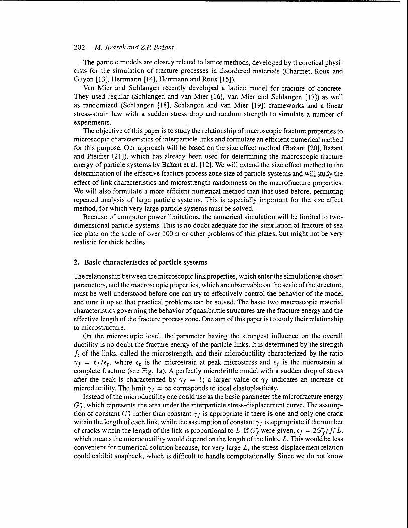
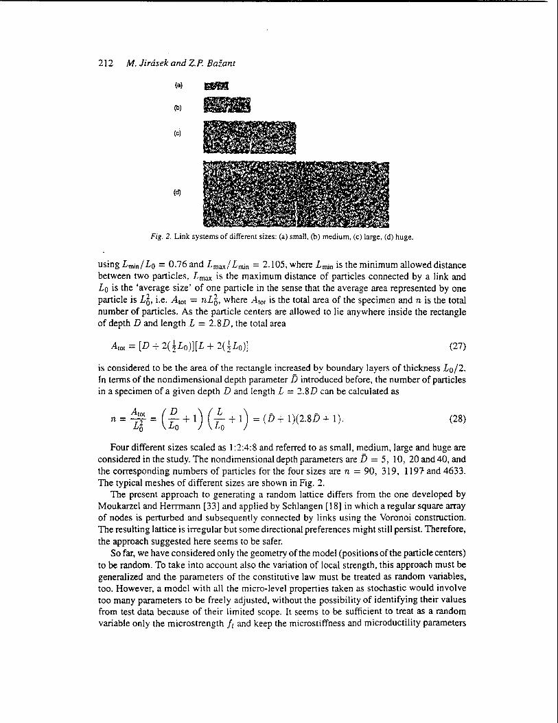
Fig. 2. Link systems of different sizes: (a) small, (b) medium, (c) large. (d) huge.

using Lmin/ La = 0.76 and Lmax/ Lmin = 2.105, where Lmin is the minimum allowed distance between two particles, Lmax is the maximum distance of particles connected by a link and La is the 'average size' of one particle in the sense that the average area represented by one particle is L6, i.e. Atol = nL6, where Atol is the total area of the specimen and n is the total number of particles. As the particle centers are allowed to lie anywhere inside the rectangle of depth D and length L = 2.8D, the total area

A lol = [D + 2(~Lo)][L + 2nLo)] - - (27)

is considered to be the area of the rectangle increased by boundary layers of thickness Lo/2. In terms of the nondimensional depth parameter jj introduced before, the number of particles in a specimen of a given depth D and length L = 2.8D can be calculated as

Alol ( D ) ( L ) -, -n= L6 = La +1 La +1 =(DT1)(2.8D+l). (28)

Four different sizes scaled as 1 :2:4:8 and referred to as small, medium, large and huge are considered in the study. The nondimensional depth parameters are jj = 5, 10, 20 and 40, and the corresponding numbers of particles for the four sizes are n = 90, 319, 1191 and 4633. The typical meshes of different sizes are shown in Fig. 2.

The present approach to generating a random lattice differs from the one developed by Moukarzel and Herrmann [33] and applied by Schlangen [18] in which a regular square array of nodes is perturbed and subsequently connected by links using the Voronoi construction. The resulting lattice is irregular but some directional preferences might still persist. Therefore, the approach suggested here seems to be safer.

So far, we have considered only the geometry of the model (positions of the particle centers) to be random. To take into account also the variation of local strength, this approach must be generalized and the parameters of the constitutive law must be treated as random variables, too. However, a model with all the micro-level properties taken as stochastic would involve too many parameters to be freely adjusted, without the possibility of identifying their values from test data because of their limited scope. It seems to be sufficient to treat as a random variable only the microstrength it and keep the microstiffness and microductility parameters

Macroscopic fracture characteristics 213

fixed. The distribution of microstrength should clearly be asymmetric because only positive values can be allowed. As no detailed information about the distribution can be deduced from tests, a simple log-normal law with only two parameters is the most convenient choice. This means that the logarithm of microstrength has a normal distribution and the values of microstrength for individual links can be obtained by exponentiating a generated sequence of random numbers with a normal distribution. The resulting distribution of microstrength can be characterized by its mean value it and coefficient of variation w 1. In the definition of the normalized nominal strength and of the normalized fracture energy (3), as well as in (4), the deterministic strength it will be replaced by the mean value it.

Figure 1 c shows the probability density for distributions with it = 0.4 MPa and w 1 = 20%, 40% and 60%, respectively. In general, a spatial correlation function for microstrength could be introduced to model stronger and weaker regions larger than the size of one particle. To keep things simple, no spatial correlation is taken into account in this study.

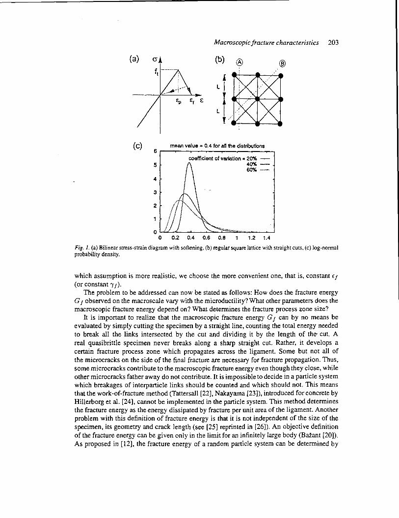
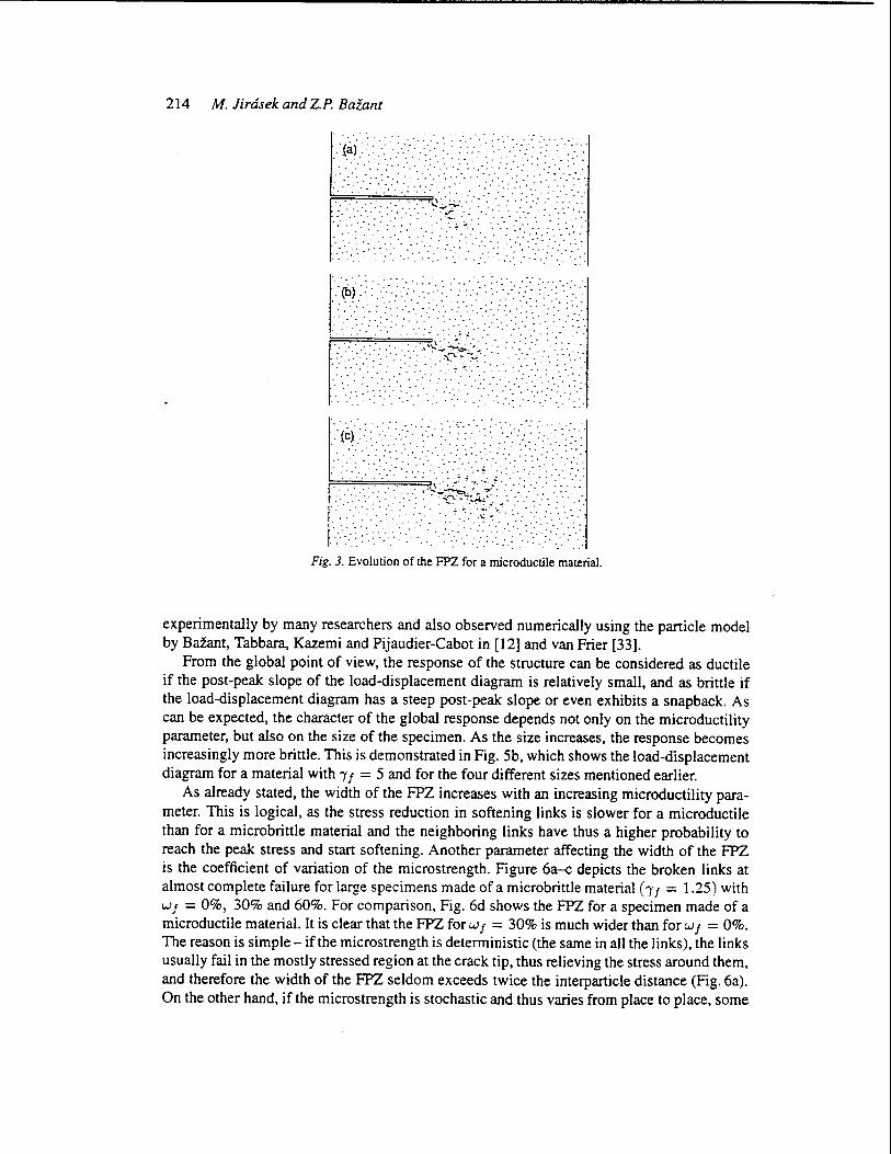
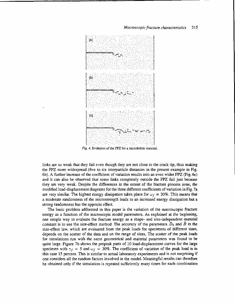
Typical results are illustrated by the load-displacement diagrams and by the plots of the (racture process zone (FPZ) at different stages of damage evolution in Fig. 3 and 4. Both examples have been constructed for a model with deterministic microstrength (1...,'1 = 0), Figure Sa shows the load-displacement diagram for a huge specimen with a highly ductile constitutive law (;1 = IS). Note that the solution procedure outlined in the previous section handles snapback without any need for introducing special measures and the load-displacement diagram can be followed far beyond its peak. The extent of the FPZ at peak load is shown in Fig. 3a and the evolution after peak in Fig. 3b,c. The dots mark the particle centers, and the lines are perpendicular to the damaged links. At the peak, all the damaged links are still softening (no links are broken yet), while at later stages, both softening and broken links exist. The full depth of the specimen is covered by the plot, but the regions around the supports have been cut off. Figure Sc indicates that the character of the load-displacement diagram for a microbrittle material (;1 = 1.2S) is grossly different from the diagram for a microductile material (Fig. Sa). Every link that starts softening breaks very soon (usually right in the next step) and so there are hardly any softening links in the FPZ at any stage of its development. At the point at which a link starts softening, the load-displacement diagram snaps back very sharply and both the load and the displacement decrease considerably, but when the softening link breaks, the load can increase again until another link starts softening. The global stiffness represented by the slope of the load-displacement diagram gradually decreases, and so do the local peak values of the load. Of course, this type of the diagram can never be observed in an experiment, because the branch snapping back is unstable and cannot be followed by the real system. The loss of stability at the peak leads to a dynamic process because static equilibrium cannot be maintained anymore under displacement control. However, if the damping is sufficient and the drop to the next branch is not very deep, static equilibrium might be restored again and the process might continue in a stable way until the next local peak is reached. Figure Sd shows a modified load-displacement diagram constructed from the diagram in Fig. Sc by replacing the unstable branches snapping back by vertical drops to the next stable branch. This type of visual representation makes it easier to compare the response for different combinations of parameters.

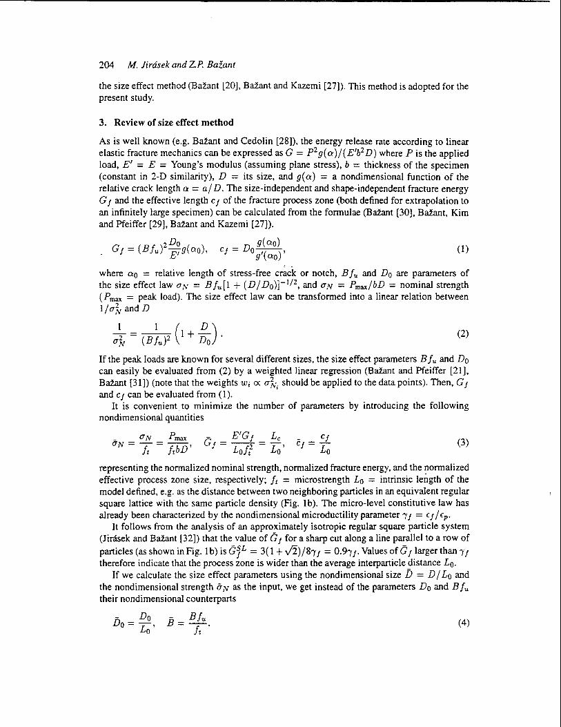
Figure 4 shows the FPZ for a microbrittle material at different stages of evolution. Com­pared to Fig. 3, it is clear that a microbrittle material produces a narrower FPZ than a micro­ductile one. It is also interesting to observe that a continuous 'crack' is not formed right away and that several small isolated groups of links in the FPZ can still carry some forces across the crack. This is a manifestation of the well-known phenomenon of crack bridging observed

214 M. lirasek and 2.p. Bazan!

.' ·.(iti. : :'.:: .. :-:': . . ', ' ..... ,', .. "'.,' ... , ,' .

. '. ,' ... ?=='=,====';i:::' . =,:;' •• ~: ..... : '. • '.: :.:.-.... • • • • • '.' •

':.":'.':'.::": : .. : ........ ~:.t::··:.·:· >.'.:.'.:. :::.;' :': ........ : '. '... . ~ ~".'-: . ~ ..... ~. :,~, :'. ". :'" , ...... .' .. : .'., .... ".

. . '. .: .... , . . '., .

, . . . . . . . " . '.' .. ' .. , .. ', .

. . .. !c) ~ --. : .' : .:. ' ....

.... : ...... .

. .- .'. : : ... ' .. . . ..

. .. . . '

. . "

.. , ...

, .'. '.' '. '" ' .. ~. '.: . . ,,' .

':::.>.:. ~'. :'.:':' ... : ~. ~~#Z~~C :.':/::'<::'" .:::. '~-::'. . '\;-..... . '.

", ..... . , ... '.

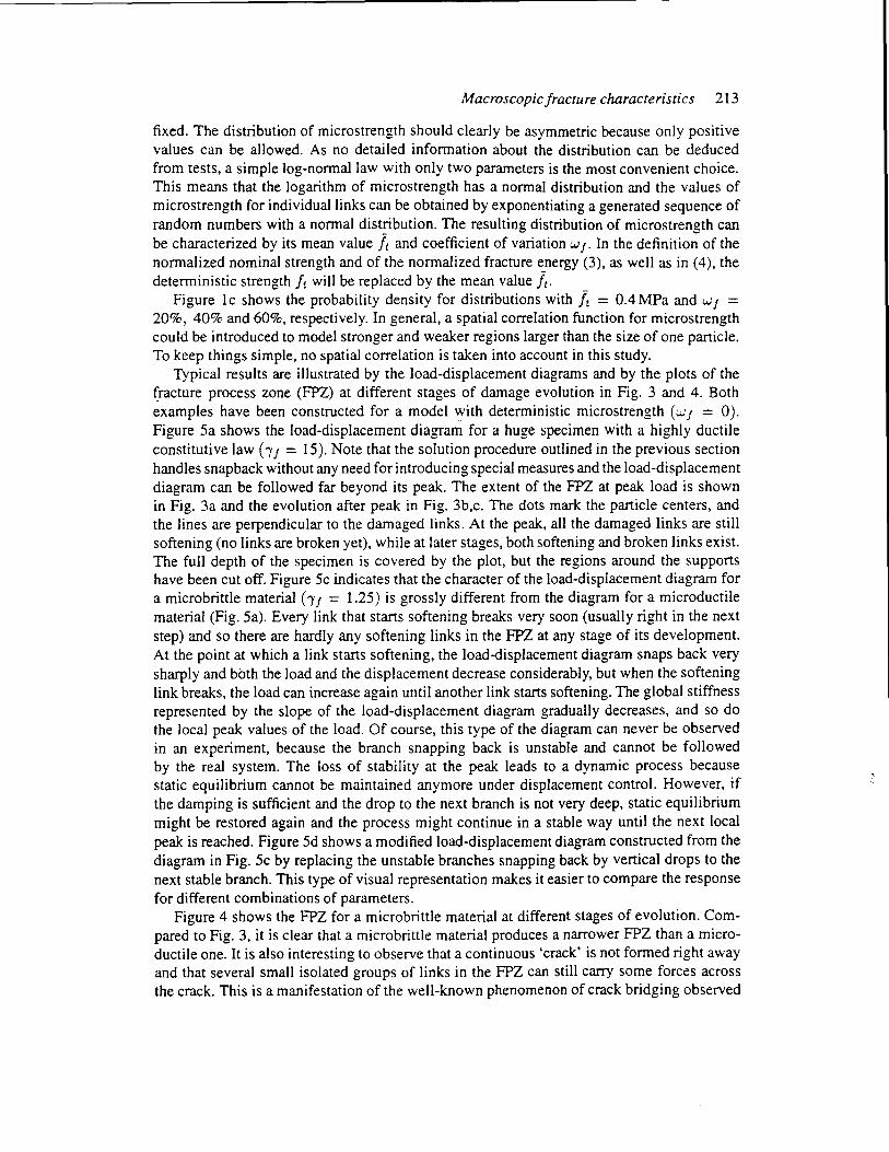
Fig. 3. Evolution of the FPZ for a microductile material.

experimentally by many researchers and also observed numerically using the particle model by Bafant, Tabbara, Kazemi and Pijaudier-Cabot in [12] and van Frier [33].

From the global point of view, the response of the structure can be considered as ductile if the post-peak slope of the load-displacement diagram is relatively small, and as brittle if the load-displacement diagram has a steep post-peak slope or even exhibits a snapback. As can be expected, the character of the global response depends not only on the microductility parameter, but also on the size of the specimen. As the size increases, the response becomes increasingly more brittle. This is demonstrated in Fig. 5b, which shows the load-displacement diagram for a material with 'Y J = 5 and for the four different sizes mentioned earlier.

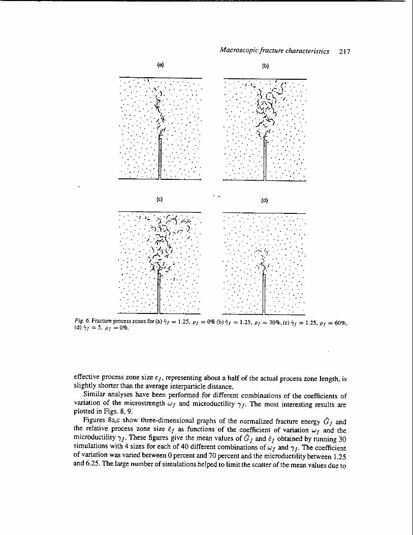
As already stated, the width of the FPZ increases with an increasing microductility para­meter. This is logical, as the stress reduction in softening links is slower for a microductile than for a microbrittle material and the neighboring links have thus a higher probability to reach the peak stress and start softening. Another parameter affecting the width of the FPZ is the coefficient of variation of the microstrength. Figure 6a~ depicts the broken links at almost complete failure for large specimens made of a microbrittle material ('Y f = 1.25) with wf = 0%, 30% and 60%. For comparison, Fig. 6d shows the FPZ for a specimen made of a microductile material. It is clear that the FPZ for W J = 30% is much wider than for W f = 0%. The reason is simple - if the microstrength is deterministic (the same in all the links), the links usually fail in the mostly stressed region at the crack tip, thus relieving the stress around them, and therefore the width of the FPZ seldom exceeds twice the interparticle distance (Fig. 6a). On the other hand, if the microstrength is stochastic and thus varies from place to place, some

Macroscopic fracture characteristics 215

" .' ... ' .' : ..... ,"", . ..... ,', . . . ....

. ,"' '.

': ':.'.',: .. ':-:'" . .':" ~0j": : .. ~ :,':'~.: ' .. ' .. " , .' . '. ' .. . " .:' : .' . ' ..... ,' ... :., .

. . :. . . .' . '., . . .. . .' :.: ...... : .. . . . " , ..

.... . •...•.•... •.....• ... ..... ... •... ••. '''--'~>-<\i . " ,- .. :...... . ....... .

...... ', '" . . " '"

. .' . ', ... ',. """',,: .', .. .. (~) :,'>., .' ...... ' ...... '.' :.: .. :: ,:.,:' .

. . . ' .: '. .' ' .. . . " . : : .' .. . '"

.:-.':'.: ::, :<":'."':~~'~~~:>~~:>:~"~~~: :' . . ',' ':' ': .' .... '. .' . . . ' .. - .. . . . . .... ', .. " "

", . . .. ' .. , .. . '. . . "': "

Fig. 4. Evolution of the FPZ for a microbrittle material.

links are so weak that they fail even though they are not close to the crack tip, thus making the FPZ more widespread (five to six interparticle distances in the present example in Fig. 6b). A further increase of the coefficient of variation results into an even wider FPZ (Fig. 6c) and it can also be observed that some links completely outside the FPZ fail just because they are very weak. Despite the differences in the extent of the fracture process zone, the modified load-displacement diagrams for the three different coefficients of variation in Fig. 7a are very similar. The highest energy dissipation takes place for W f = 30%. This means that a moderate randomness of the microstrength leads to an increased energy dissipation but a strong randomness has the opposite effect.

The basic problem addressed in this paper is the variation of the macroscopic fracture energy as a function of the microscopic model parameters. As explained at the beginning, one simple way to evaluate the fracture energy as a shape- and size-independent material constant is to use the size-effect method. The accuracy of the parameters Do and iJ in the size-effect law, which are evaluated from the peak loads for specimens of different sizes, depends on the scatter of the data and on the range of sizes. The scatter of the peak loads for simulations run with the same geometrical and material parameters was found to be quite large. Figure 7b shows the prepeak parts of 10 load-displacement curves for the large specimen with If = 5 and wf = 30%. The coefficient of variation of the peak load is in this case 15 percent. This is similar to actual laboratory experiments and is not surprising if one considers all the random factors involved in the model. Meaningful results can therefore be obtained only if the simulation is repeated sufficiently many times for each combination

216 M. lirasek and z.P. Bazant

(a) 10

9

8 7

6

'" III 5 .2 4

3

2 1

0 0 0.01 0.02 0.03 0.04

displacement

ic) 5,---.---.--.----.---..:-.----.---.---,.---,

4.5

4

3.5

3

] 2.5

2 1.5

5

4

3

2

huge -large -

medium '-' small-

o~-~---==~-----'--~ o 0.005 0.01 0.015 0.02 0.025 0.03

displacement

5 (d)

4.5

4

3.5 . 3

2.5

2

1.5

Q5 Q5 o 0 L--,---,-_,---,---,-~,---,----,-_o....-.-J

o 0.020.040.060.080.1 0.120.140.160.180.2 0 0.020.040.060.08 0.1 0.120.140.160.180.2 displacement displacement

Fig. 5. Load-displacement diagram (a) for a microductile model, (b) for different sizes, (c-<J) for a microbrittle model.

of parameters considered, so that the mean value of the peak load can be computed with a reasonable accuracy. The advantage of the numerical simulation as compared to the laboratory experiment is that the number of tests is limited only by the available computer time. Another factor significantly contributing to the reliability of the results is the range of sizes used for the size-effect evaluation. The largest specimen used in this study is eight times larger than the smallest one so that a sufficiently wide range of sizes be covered.

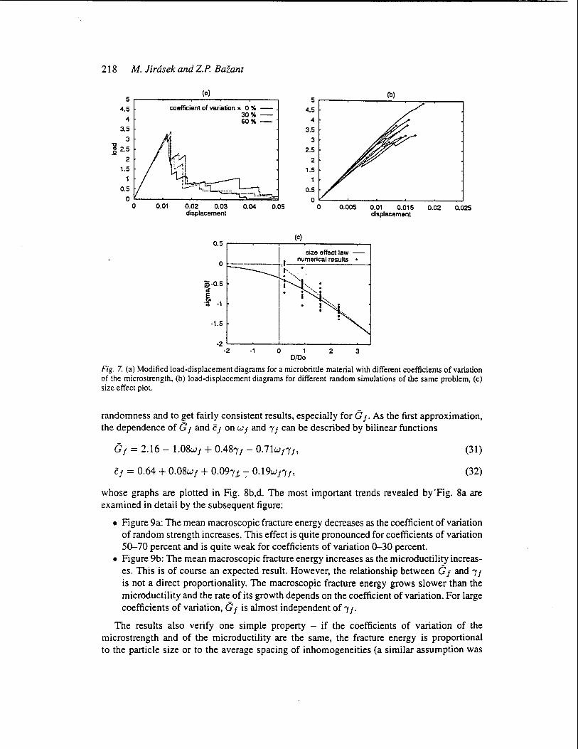
Figure 7c shows the size-effect plot of all the (IN values for 'f = 2.5 and wf = 10%. The simulated normalized nominal strengths aN for 20 specimens of each size are plotted, along with the theoretical curve corresponding to the size-effect law proposed by BaZant [30]. As expected, the scatter of the individual results is quite large but the mean (IN values follow the theoretical curve very closely. Based on the nondimensional size-effect parameters Do = Dol Lo = 4.071 and fJ = Bful It = 0.1846, the fracture energy and the relative process zone size are evaluated according to (5)

- - -2 2 Gj = g(o:o)DoB = 20.27 x 4.071 x 0.1846 = 2.81, (29)

_ g(ao) - 20.27 cf = gl(o:o)Do = 113.1 x 4.071 = 0.73. (30)

These results mean that the macroscopic fracture energy is slightly larger than the energy corresponding to a straight cut in a square lattice, for which GJL = 0.9, j = 2.25 and the

(a)

. . .

(e)

..... /: \~ .. " . r.:..<. .....

. . . '. . ';I. ,7" . } . /-:1--. . . .. \- ) ' ... : .' : .' ''':~~~''\ ~/~ .' : : .. . ' . . . . /. ';.,.-J . .. / . . ' ..... .... '1~ . " .. : . .. '. \ "'}'~; i' . . · '. . .... i~': '''f . . .

· :. .: .. , .... :.--: I· ':.' . . . . · . '. ' . . )t. '/.{.' . . . . ) . '. . .... ,,- ',':' . .... ..... . ,. ' ..

. . ' . . · ... , .

Macroscopic fracture characteristics 217

, ,

(b)

.. ' .

Cd)

. ...

.. ' .. ' ..

. . ' .

Fig. 6. Fracture process zones for (a) 7, = 1.25, p, = 0% (b) 7, = 1.25, P, = 30%. (c) 7, = 1.25, p, = 60%, (d) 7, = 5, P, = 0%.

effecti ve process zone size C J' representing about a half of the actual process zone length, is slightly shorter than the average interparticle distance.

Similar analyses have been performed for different combinations of the coefficients of variation of the microstrength W J and microductility J J. The most interesting results are plotted in Figs. 8, 9.

Figures 8a,c show three-dimensional graphs of the normalized fracture energy (; J and the relative process zone size C J as functions of the coefficient of variation W J and the microductility 'Y J. These figures give the mean values of (; J and C J obtained by running 30 simulations with 4 sizes for each of 40 different combinations of W J and J J. The coefficient of variation was varied between 0 percent and 70 percent and the microductility between 1.25 and 6.25. The large number of simulations helped to limit the scatter of the mean values due to

218 M. lirasek and Zp. Bazant

(a) 5 .---~----~----~----~--~

4.5

4

3.5

3

~ 2.5 2

1.5

1

0.5

coefficient of variation - 0 % -30%-60% --

o ~--~----~----~--~----~

5r---~----~~~)~--~~---, 4.5

4

3.5

3

2.5

2 1.5

1

0.5

O~--~----~--~----~--~ o 0.01 0.02 0.03 displacement

0.04 0.05 o 0.005 0.01 0.Q15 0.02 0.025 displacement

(c) 0.5 r---~----"------'-----'----~--'

o

~.0.5

.~ ·1

·1.5

I size effect law -. ___ -;. .. r~_merical results •

I", • 1 !"'< .

'.

·2~--~--~----~--~----~ ·2 ·1 o 1 2 3

DIDo

Fig. 7. (a) Modified load·displacement diagrams for a microbrittle material with different coefficients of variation of the microstrength, (b) load-displacement diagrams for different random simulations of the same problem, (c) size effect plot.

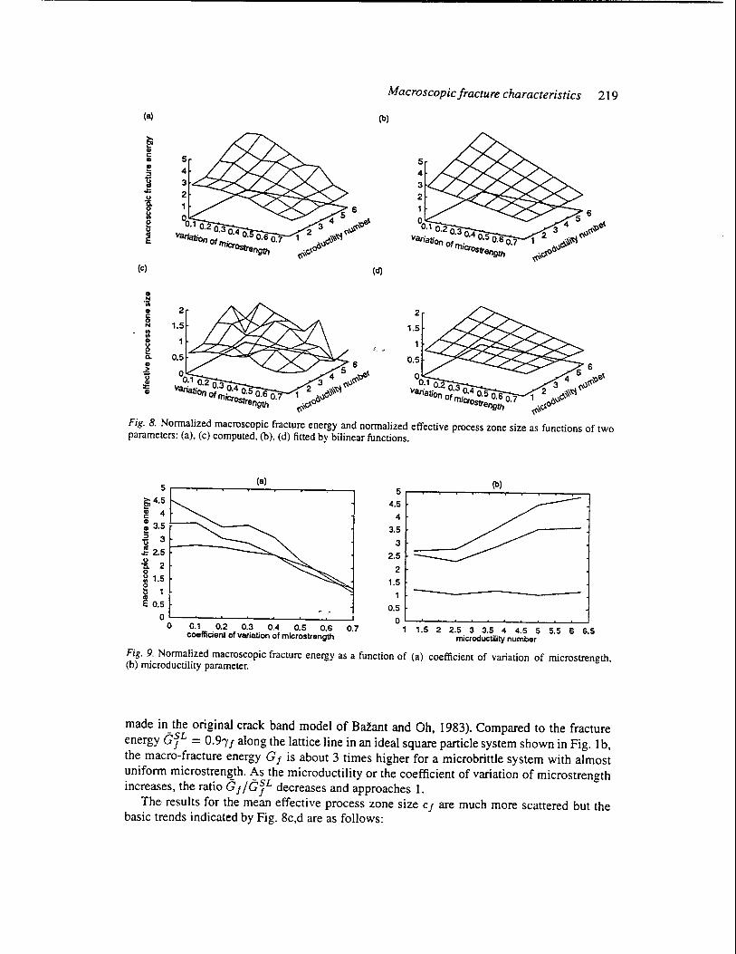
randomness and to get fairly consistent results, especially for G f. As the first approximation, the dependence of G f and c 1 on W 1 and "11 can be described by bilinear functions

G f = 2.16 - 1.0Swf + 0.48"11 - 0.71wj"/1,

cf = 0.64 + O.OSwf + 0.09"1£ -; 0.19wj"/h

(31)

(32)

whose graphs are plotted in Fig. 8b,d. The most important trends revealed by·Fig. 8a are examined in detail by the subsequent figure:

• Figure 9a: The mean macroscopic fracture energy decreases as the coefficient of variation of random strength increases. This effect is quite pronounced for coefficients of variation 50-70 percent and is quite weak for coefficients of variation 0-30 percent.

• Figure 9b: The mean macroscopic fracture energy increases as the microductility increas­es. This is of course an expected result. However, the relationship between G 1 and "11 is not a direct proportionality. The macroscopic fracture energy grows slower than the microductility and the rate of its growth depends on the coefficient of variation. For large coefficients of variation, (; f is almost independent of "If.

The results also verify one simple property - if the coefficients of variation of the microstrength and of the microductility are the same, the fracture energy is proportional to the particle size or to the average spacing of inhomogeneities (a similar assumption was

Macroscopic fracture characteristics 219

(a) (b)

6 1 5 6 4 5 :r:P 0

3 4 ~'Oe( 2 3 , ~ .. .>~ 0.10.203 1 6'1.'~ 'Variati . 0.4 0.5 0.6 0 7 1 2 .~~~,)

'r:,(cP" on of rn' . .~,)~ ~~

IcrOStrength ~~

(e) (d)

2 2

1.5 1.5

- ,

6 5 6 0 4 5 :r:P 0 4 ~e( 0.10.203 3 , ~,)~ 0.10.203 3 . ~,)~ Varia . 0.4 1 2 ,)6'1.~ van· . 04 05 1 2 6~~ tion of rn' 0.5 0.6 0.7 atlon of rn;' . 0.607

1CT000rength 'r:,(cIS crostrength . 06" ~~ i-'o

Fig. 8. Normalized macroscopic fracture energy and normalized effective process zone size as functions of two parameters: (a), (c) computed. (b). (d) fitted by bilinear functions.

(a) 5r---~--T---T---~--~--~ __ ,

En 4.5

~ 4 : 3.5 :; 3 u jg 2.5 I----_~.

-[ 2 o ~ 1.5 o t 1

E 0.5

O~~---'--"""""_"'----_.L...-----'_.....J

o 0.1 0.2 0.3 0.4 0.5 0.6 0.7 coeffic:ient of variation of microstrength

(b) 5 ~~-r~--r-~~~--r-~-r~

4.5

4

3.5

3

2.5

2 1.5

0.5 o ~~~--~~~~--~~~ __ ~~

1 1.5 2 2.5 3 3.5 4 4.5 5 5.5 I) 6.5 mieroduc:tility number

Fig. 9. Normalized macroscopic fracture energy as a function of (a) coefficient of variation of microstrength, (b) microductility parameter.

made in the original crack band model of BaZant and Oh, 1983). Compared to the fracture energy G? = 0.9, f along the lattice line in an ideal square particle system shown in Fig. 1 b, the macro-fracture energy G f is about 3 times higher for a microbrittle system with almost unifonn microstrength. As the microductility or the coefficient of variation of microstrength increases, the ratio G f / G? decreases and approaches 1.

The results for the mean effective process zone size C f are much more scattered but the basic trends indicated by Fig. 8c,d are as follows:

220 M. lirasek and ZP. Baiant

• For microbrittle materials, the effective process zone size is independent of micro strength variation. For microductile materials, this size decreases as the coefficient of variation of microstrength increases .

• The effective process zone size increases as the microductility increases. However, this increase is less than proportional, and is very slow for materials with a large variation of microstrength.

6. Conclusions

1. Random particle systems characterized by a particle interaction law with softening char­acteristics realistically simulate fracture of quasibrittle materials. They exhibit large zones of distributed cracking and the particle structure acts as a localization limiter. The parti­cle system reflects the microstructure of aggregate materials such as concrete. However, because of the nature of their fracture behavior, particle systems can also be used for con­venient simulation of fracture of quasi brittle materials that do not consist of well-defined particles, in which case the particle size reflects the spacing of dominant inhomogeneities of the quasibrittle material.

2. Calculation of macroscopic fracture parameters from given microstructural properties represents a fundamental problem of micromechanics of brittle and quasibrittle materials. As proposed before, the macroscopic fracture energy can be obtained according to the size effect method. The method can also be used to determine the dependence of the mean macro-fracture energy on the statistics of the microscopic properties, such as the coeffi­cients of variation of the microstrength of the interparticle links, and on the microductility of these links.

3. The size effect method can further be used to determine the effective process zone size of a particle system and its dependence on the aforementioned microscopic properties.

4. For two-dimensional particle systems, the ratio of macro-fracture energy to the fracture energy of idealized square lattice of particles for straight-line fracture parallel to a lattice line varies approximately from 1 to 3. The effective process zone size varies approximately from 0.5 to 2 times the average interparticle distance.

5. At constant average microstrength and microductility, the macro-fracture energy is propor­tional to the average particle spacing. It decreases with increasing coefficient of variation of microstrength (or micro-fracture energy) and increases with increasing microductil­ity. The latter increase, however, weakens with increasing coefficient of variation of microstrength. It follows that in order to manufacture a quasibrittle material of high fracture energy, the properties of the individual inhomogeneities should be as uniform as possible and the size of inhomogeneities as large as possible while at the same time the microductility should be maximized (e.g. by inhibiting sudden formation of large microcracks ).

6. An efficient solution algorithm for the response of the particle system is required. Using a bilinear force-displacement diagram for each link, such an algorithm is obtained by (1) using a variable loading step from one change of status of interparticle link to another, and (2) replacing changes of the stiffness matrix due to particle link breaks by inelastic forces, which makes it possible to use the initial elastic stiffness matrix.

7. The particle simulation should be helpful especially for materials such as sea ice plates in which the dominant inhomogeneity spacing (spacing of thermal cracks, spacing of

Macroscopic fracture characteristics 221

2.5

0.5

(a)

234 567 8 displacement

2.5

T 2 !. ~ 1.5

.;aE.

0.5

p

Ilnk1 -link 2 -link 3 .-. link 4 -

2345678 extension (straln)

Fig. 10. (a) Example of a simple one-dimensional problem, (b) load-displacement diagram, (c) evolution of axial forces in individual links.

wanner zones under snowdrifts, etc.) is so large that it would require specimens larger than feasible for laboratory tests.

Appendix - Example of numerical solution

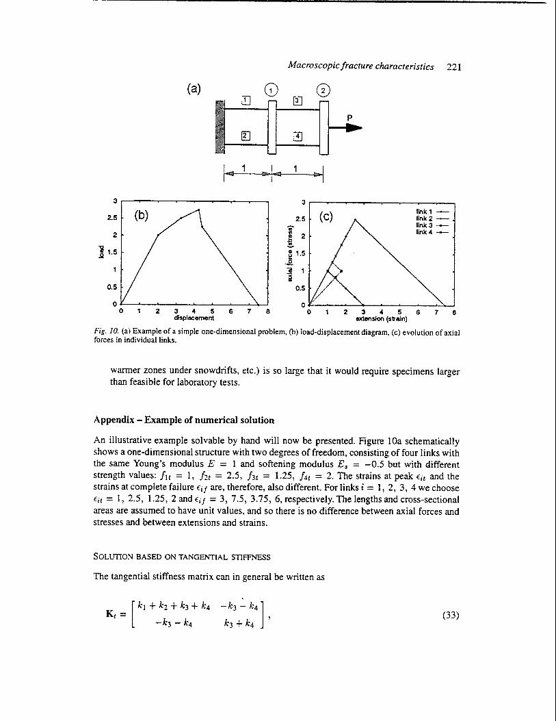
An illustrative example solvable by hand will now be presented. Figure lOa schematically shows a one-dimensional structure with two degrees of freedom, consisting of four links with the same Young's modulus E = 1 and softening modulus Es = -0.5 but with different strength values: fit = 1, ht = 2.5, ht = 1.25, f4t = 2. The strains at peak Eit and the strains at complete failure EiJ are, therefore, also different. For links i = 1, 2, 3, 4 we choose Eit = 1, 2.5, 1.25, 2 and EiJ = 3, 7.5, 3.75, 6, respectively. The lengths and cross-sectional areas are assumed to have unit values, and so there is no difference between axial forces and stresses and between extensions and strains.

SOLUTION BASED ON TANGENTIAL STIFFNESS

The tangential stiffness matrix can in general be written as

(33)

222 M. lirdsek and z.P. Bazant

where ki is the current stiffness of link i. The'reference load vector is given by

(34)

and the load parameter P is equal to the force applied at note 2.

STEP 1:

Status = (1,1,1, 1);

EI,O = 0, 8EI,1 = 0.5, fl,er =flt == 'I, 1-0

flPl 1 = -- = 2 , 0.5 '

f2,0 = 0, 8f2,1 = 0.5, f2,er = f2t = 2.5, flP2,1 = 2.5 - 0 = 5,

0.5

f3,0 = 0, 8f3,1 = 0.5, f3,er = E3t = 1.25, flP3,1 = 1.25 - 0 = 2.5,

0.5

8f4,1 = 0.5, 2-0

f4,0 = 0, f4,er = f4t = 2, flP41 = -- = 4 , 0.5 '

Link 1 changes status from 1 to 2 (starts softening).

STEP 2:

Status = (2, 1, 1, 1); kl = -0.5, k2 ~ k3 = k4 = 1,

[ 2.5 -2] { 2 } Kt2 = ====> 8d l = ,

-2 2 2.5

fl,1 = 1, 8fl,2 = 2, EI,er = flf = 3, flPI,2 = 1,

f2,1 = 1, 8f2,2 = 2, f2,cr = f2t = 2.5, !l.P2,2 = 0.75,

E3,1 = 1, 8f3,2 = 0.5, f3,er = f3t = 1.25, flP3,2 = 0.5,

£4,1 = 1, 8f4,2 = 0.5, E4,er = f4t = 2, flP4,2 = 2,

MacroscopicJracture characteristics 223

tlP2 = 0.5, P2 = 2.5, d2 = { 2 }. 3.25

Link 3 changes status from 1 to 2 (starts softening).

STEP 3:

Status = (2, 1, 2, 1);

Kt3 = [ 1 -0.5

==> bd3 = , -0.5] { 2 } 0.5 4

EI,2 = 2, bEI,3 = 2, EI,cr = Ell = 3,

E2,2 = 2, bE2,3 = 2, E2,cr = E2t = 2.5,

E3,2 = 1.25, 15103,3 = 2, E3,cr = E31,=: 3.75,

104,2 = 1.25, 15104,3 = 2, f4,cr = E4t = 2,

.6.yi = tlP2,3 = 0.25; tlP3- not defined,

.6.P3 = 0.25, P3 = 2.75, {

2.5 } d3 = . 4.25

Link 2 changes status from 1 to 2 (starts softening).

STEP 4:

Status = (2, 2, 2, 1);

K = [-0.5 -0.5] t4 -0.5 0.5

101,3 = 2.5, 15101,4 = -1,

102,3 = 2.5, bE2,4 = -1,

E3,3 = 1.75, 15103,4 = 2,

104,3 = 1.75, 15104,4 = 2,

EI,cr = flf = 3,

E2,cr = E21 = 7.5,

E3,cr = f3f = 3.75,

f4,cr = f4t = 2,

tlPI,3 = 0.5,

tlP2,3 = 0.25,

tlP3,3 = 1.25,

tlP4,3 = 0.375,

tlPI,4 = -0.5,

6.P2,4 = -5,

6.P3,4 = 1,

6.P4,4 = 0.125,

Links 1 and 2 are negative, link 3 is positive. As there exist more negative links than positive ones, it is expected that 6.P4 will have a negative sign. In that case, strain in link 3 would decrease, which is not consistent with the assumption that this link is softening. Its status must be changed to 5 and the increment must be recalculated:

Status = (2, 2, 5, 1); kl = k2 = -0.5, OJ 1

k3 = - = - = 0.571 k4 = 1, 103 1.75

224 M. Jirtisek and 2.p. Bazant

[ 0.571 K -t4 - -1.571

-1.571 1 1.571

~ 6~ = { =~.364 } ,

fl,3 = 2.5, 6fl,4 = -1, fl,cr = fll = 3, LlPI ,4 = -0.5,

f2,3 = 2.5, 6f2,4 = -1, f2,cr = f21 = 7.5, LlP2,4 = -5,

f3,3 = 1.75, 6'€3,4 = 0.636, €3,cr = f3,3 = 1.75, LlP3,4 = +0,

f4,3 = 1.75, 6'f4,4 = 0.636, f4,cr = €4t = 2, LlP4,4 = 0.393,

Now, all three links 1, 2, 3 are negative, because a negative increment of LlP gives strain increments consistent with the assumptions (positive in softening links 1, 2, negative in the ~nloading link 3). An admissible solution is found for LlP = LlP4- = -0.5:

!>P, = -0.5, P, = 2.25, <4 = { 4.:3~ }.

Link 1 changes status from 2 to 4 (breaks completely). Link 3 is transferred from status 5 to status 3.

STEP 5:

Status = (4, 2, 3, 1); kl = 0, k2 = -0.5, k3 = 0.571, k4 = 1,

[ 1.071

Kts = -1.571

fl,4 = 3,

f2,4 = 3,

f3,4 = 1.432,

f4,4 = 1.432,

LlPs = -2.25,

-1.571] 1.571

6'fl,S = -2,

6'f2,S = -2,

6'f3,S = 0.636,

6f4,S = 0.636,

Ods = { =~.364 },

fl,cr not defined

f2,cr = f21 = 7.5, LlP2,s = -2.25,

f3,cr = f3,max = 1.75, LlP3,s = 0.5,

f4,cr = f4t = 2, LlP4,s = 0.893,

Ps = 0, { 7.5} ds = . 7.5

Link 2 is negative and so only LlPs- leads to an admissible solution. Link 2 changes status from 2 to 4 (breaks completely).

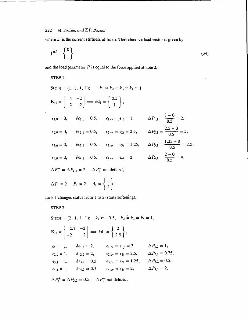
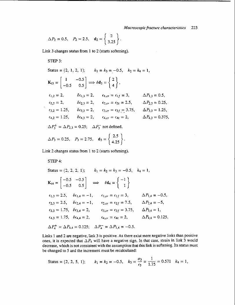
At the end of the fifth step, links 1 and 2 are broken, while links 3 and 4 are unloaded to zero stress and strain - link 3 after some damage, link 4 still in the virgin state. The global load-displacement diagram is plotted in Fig. lOb and diagrams showing the evolution of stress and strain (axial force and extension) in individual links are plotted in Fig. 10c.

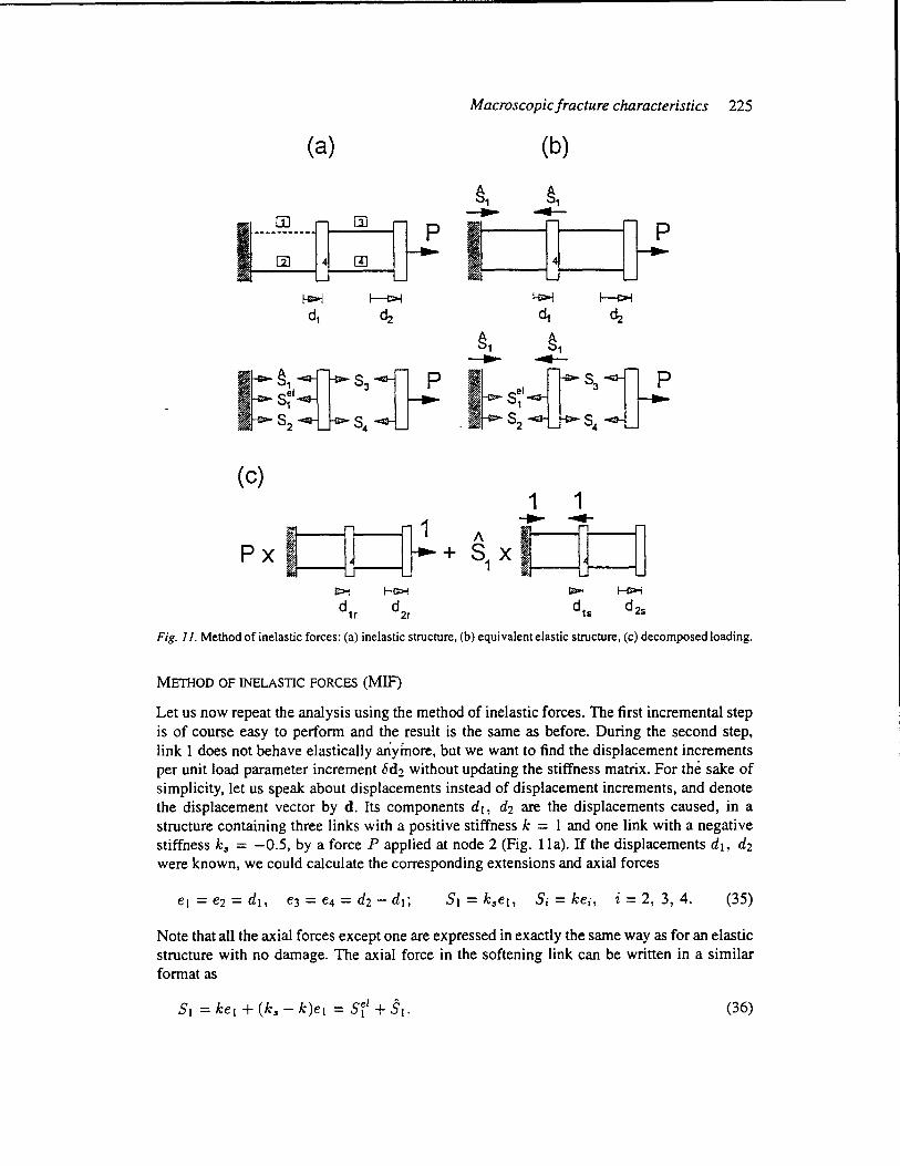
(a)

I----:---D rn

[}! rn

f-C>j r-t>! d, ~

(c)

Px I ~ f+ I>i I--!>l

d,r d 2r

Macroscopic fracture characteristics 225

~1 ~

I ~1 ~

(b)

~1 ~

~ [}! H>i f-i>i d, ~

1: ..... S~I:D:S3]! S .. .. S . '. 2 4

1 1

--- ~ A I ~ ~ S1 X

~ H>i

d,s d 2s

Fig. 11. Method of inelastic forces: (a) inelastic structure, (b) equivalent elastic structure, (c) decomposed loading.

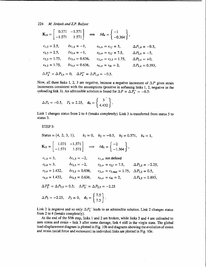
METHOD OF INELASTIC FORCES (MIF)

Let us now repeat the analysis using the method of inelastic forces. The first incremental step is of course easy to perfonn and the result is the same as before. During the second step, link 1 does not behave elastically anymore, but we want to find the displacement increments per unit load parameter increment bd2 without updating the stiffness matrix. For the sake of simplicity, let us speak about displacements instead of displacement increments, and denote the displacement vector by d. Its components d1, d2 are the displacements caused, in a structure containing three links with a positive stiffness k = 1 and one link with a negative stiffness ks = -0.5, by a force P applied at node 2 (Fig. lla). If the displacements dI, d2 were known, we could calculate the corresponding extensions and axial forces

(35)

Note that all the axial forces except one are expressed in exactly the same way as for an elastic structure with no damage. The axial force in the softening link can be written in a similar fonnat as

(36)

226 M. lirdsek and z.P. Bazant

The fictitious force

(37)

represents the difference between the real axial force SI and the axial force Sit that would exist under the same extension if the link remained elastic, and is therefore called the inelastic force. Combining the first strain-displacement equation from (35) with (37) derived from the constitutive law, we get a relationship between the inelastic force 51 and the displacements, similar to (21)

(38)

As neither the inelastic force nor the displacements are known, (38) cannot be sol ved separately and seems to be nothing more than a definition of 51. However, we can now look at the equilibrium of the structure and supplement (38) by another equation relating 51 to d 1.

The key idea is that we can replace the structure with one softening link, internal forces SI = Sit + 51, S2, S3, S4, and external force P (Fig. lla) by an elastic structure with internal forces Sit, S2, S3, S4 and external forces 51, P (Fig. 11 b). Clearly, the structure in Fig. 11 b satisfies all basic equations: equilibrium, because the free body diagrams in Figs. 11 a and 11 b are the same, strain-displacement equations and the constitutive law, because all the internal forces are computed from the displacement in the same way as for an elastic structure. Hence the displacements d l , d2 can be expressed in terms of 51 and P by solving the elastic structure in Fig. 11 b, which is easy, as the elastic stiffness matrix is known. For convenience, let us represent the loading in Fig. 11 b as a superposition of a P-multiple of the reference loading and a 51-multiple of a pair of unit forces (Fig. IIc). Mathematically, the problem is described by

Kod = Pf ref + 5tl, (39)

which is a special form of (20). The displacements caused by the reference loading f ref will be denoted by riff, dr.{f, and the displacements caused by the unit inelastic forces by d1, d2.

Similar to (25), the actual displacements d 1, d2 are linear combinations

(40)

The first of these equations relates d1 and 51 and, when substituted into (38), yields a single equation for the inelastic force:

- - f [1 - (k s - k)dtl Sl = (k s - k)cFr P. (41)

This is a special form of the fundamental equation (26). The value of 51 calculated from (41) can be substituted into (40) to yield the displacements, and the problem is solved.

For the specific example considered here, the elastic stiffness matrix, reference loading vector and the loading vector of unit inelastic forces were shown to be

[ 4 -2] Ko = -2 2'

- _ { -1 } f- . o

Macroscopic fracture characteristics 227

Solving two systems of linear equations with the same coefficient matrix Ko and right hand sides f ref and C, we get the corresponding displacements

ref _ { 0.5 } . _ { -0.5 } d - ,d - . 1 -0.5

Equation (41) can now be written as [1 - (-0.5 - 1)(-0.5)]51 = (-0.5 - 1 )0.5P, or 0.2551 = -0.75P, from which 51 = -3P. Substituting into (40), the displacements can be computed: d l = (-0.5)( -3P) + 0.5P = 2P, d2 = (-0.5)( -3P) + LOP = 2.5P. The coefficients at P represent the displacement increments per unit increment of the loading parameter

8d2 = { 2 }. . 2.5

This result exactly agrees with the previous one, but now the tangential stiffness matrix is not used at all.

MIF IN MATRIX NOTATION

In matrix notation. the calculation can be described as follows:

[ 4 -2] Ko = , -2 2

ref _ { 0 } ref _ { 0.5 } f - ,d - . 1 1

In the first step. there are no damaged links and 8d l = dref• In the second step. link 1 is softening

B = [1 0],

0=[-1.5],

OBdref = {-0.75},

. - [-0.5] R- , -0.5

1- OBR = [0.25],

s = {-3}, 8d2 = { 2 }. 2.5

In the third step. links 1 and 3 are softening

. _ [ 1 0] B- , -1 1

. [ -0.5 0] R= -0.5 -0.5 '

0= [-1.5 0] o -1.5'

. . . [0.25 0] I - DBR = 0 0.25'

•• f {-0.75 } DBdre = -0.75 ' 5 ~ { = ~ }, Od, ~ { ~ } .

228 M. lirdsek and z.P. Bazan!

Acknowledgement

Partial financial support under AFOSR Grant 91-0140 to Northwestern University is grate­fully acknowledged. Applications to fracture analysis of sea ice plates were supported under ONR Grant N0014-91-2-11 09 to Northwestern University. Partial funding for applications to concrete has further been received from the Center for Advanced Cement-Based Materials at Northwestern University.

References

1. P.A. Cundall. in Proceedings, International Symposium on Rock Fracture, ISRM, Nancy (1971). 2. A.A. Serrano and J.M. Rodriquez-Ortiz, in Proceedings, Symposium on Plasticity and Soil Mechanics,

Cambridge. U.K. (1973). 3. J .M. Rodriguez-Ortiz, thesis, Universidad Politecnico de Madrid, Spain (1974) in Spanish. 4. T. Kawai, International Journalfor Numerical Methods in Engineering 16 (1980) 81-120. 5. P.A. Cundall. BALL-A program to model granular media using the distinct element method. Technical note,

Dames and Moore, London (1978). 6. P.A. Cundall and O.D.L. Strack, Geotechnique 29 (1979) 47-65. 7. A. Zubelewicz, thesis, Technical University of Warsaw, Poland (1990) in Polish. 8. A. Zubelewicz, Archiwum Inzynierii Ladowej 29 (1983) 417-429, in Polish. 9. A. Zubelewicz and Z. Mroz, Rock Mechanics and Engineering 16 (1983) 253-274.

10. M.E. Plesha and E.e. Aifantis, in Proceedings, 24th U.S. Symposium on Rock Mechanics, College Station, Texas (1983).

II. A. Zubelewicz and Z.P. BaZant, Journal of Engineering Mechanics ASCE 113 (1987) 1619-1630. 12. Z.P. Bazant, M.R. Tabbara, M.T. Kazemi and G. Pijaudier-Cabot, Journal of Engineering Mechanics ASCE

116(1990) 1686-1705. 13. J.e. Charmet, S. Roux and E. Guyon (eds.), Disorder and Fracture, Plenum Press, New York (1990). 14. H.J. Herrmann, Fracture Processes in Concrete, Rock and Ceramics, Chapman & Hall, New York (1991). 15. H.J. Herrman and S. Roux (eds.), Statistical Modelsfor the Fracture of Disordered Media, North-Holland.

New York (1990). 16. E. Schlangen and J.G.M. van Mier, Cement and Concrete Composites 14 (1992) 105-118. 17. J.G.M. van Mier and E. Schlangen, Journal of the Mechanical Behavior of Materials 4 (1993) 179-190. 18. E. Schlangen, PhD. thesis, Technical University of Delft, The Netherlands (1993). 19. E. Schlangen and J .G.M. van Mier, in Proceedings of Com pUla tiona I Methods in Materials Science, Materials

Research Society, Pittsburgh, Pennsylvania (1993) 153-158. 20. Z.P. BaZant. in SEM-RILEM International Conference on Fracture of Concrete and Rock, Houston, Texas,

S.P. Shah and S.E. Swartz (eds.), SEM (1987) 390-402. 21. Z.P. Bazam and P.A. Pfeiffer, ACI Materials Journal 84 (1987) 463-480. 22. H.G. Tattersall and G. Tappin, Journal of Materials Science 1:3 (1966) 296-301. 23. J. Nakayama. Journal of the American Ceramic Society 48: II (1965). 24. A. Hillerborg, M. Modeer and P.E. Peiersson, Cement and Concrete Research 6 (1976) 773-782. 25. Z.P. Bazant (ed.), Fracture Mechanics of Concrete Structures, Elsevier, London (1992). 26. Z.P. Bazant and V. Gopalaratnam, in Fracture Mechanics of Concrete Structures, Z.P. Bazant (ed.), Elsevier,

London (1992) 1-140. 27. Z.P. Bazant and M.T. Kazemi, in Conference on Advances in Cement Manufacturing and Use, E. Gartner

(ed.), (1988) Paper No.5. 28. Z.P. BaZant and L. Cedolin. Stability of Structures, Oxford University Press, New York (1991). 29. Z.P. BaZant. J.-K. Kim and P.A. Pfeiffer, Journal of Structural Engineering ASCE 112, ST2 (1986) 289-307. 30. Z.P. BaZant. Journal of Engineering and Meclzanics ASCE 110 (1984) 518-535. 31. Z.P. Bazant.MaterialsandStructures23 (1990)461-465. 32. M. Jirasek and Z.P. Bazant, Journal of Engineering Mechanics ASCE, in press. 33. C. Moukarzel and H.J. Herrmann. HLRZ 1192, HLRZ KFA Jillich, Germany (1992) preprint. 34. J.G.M. van Mier, Cement and Concrete Research 21 (1991) 1-15.