mae 5100 - continuum mechanics course notes · 2018-01-08 · lecture 1 introduction and index...
TRANSCRIPT
MAE 5100 - Continuum MechanicsCourse NotesBrandon Runnels
ContentsLECTURE 1 0 Introduction 1.1
0.1 Motivation . . . . . . . . . . . . . . . . . . . . . . . . . . . . . . . . . . . . . . . . 1.10.2 Notation . . . . . . . . . . . . . . . . . . . . . . . . . . . . . . . . . . . . . . . . . 1.2
0.2.1 Sets . . . . . . . . . . . . . . . . . . . . . . . . . . . . . . . . . . . . . . 1.20.2.2 Proof notation . . . . . . . . . . . . . . . . . . . . . . . . . . . . . . . . . 1.2
1 Tensor Analysis 1.21.1 Index notation and the Einstein summation convention . . . . . . . . . . . . . . 1.3
1.1.1 Vector equality . . . . . . . . . . . . . . . . . . . . . . . . . . . . . . . . 1.41.1.2 Inner product . . . . . . . . . . . . . . . . . . . . . . . . . . . . . . . . . 1.41.1.3 Kronecker delta . . . . . . . . . . . . . . . . . . . . . . . . . . . . . . . . 1.41.1.4 Components of a vector . . . . . . . . . . . . . . . . . . . . . . . . . . . 1.51.1.5 Norm of a vector . . . . . . . . . . . . . . . . . . . . . . . . . . . . . . . 1.51.1.6 Permutation tensor . . . . . . . . . . . . . . . . . . . . . . . . . . . . . . 1.51.1.7 Cross product . . . . . . . . . . . . . . . . . . . . . . . . . . . . . . . . . 1.51.1.8 Notation . . . . . . . . . . . . . . . . . . . . . . . . . . . . . . . . . . . . 1.6
LECTURE 2 1.2 Mappings and tensors . . . . . . . . . . . . . . . . . . . . . . . . . . . . . . . . . 2.11.2.1 Second order tensors . . . . . . . . . . . . . . . . . . . . . . . . . . . . . 2.11.2.2 Index notation . . . . . . . . . . . . . . . . . . . . . . . . . . . . . . . . . 2.11.2.3 Dyadic product . . . . . . . . . . . . . . . . . . . . . . . . . . . . . . . . 2.21.2.4 Tensor components . . . . . . . . . . . . . . . . . . . . . . . . . . . . . 2.21.2.5 Higher order tensors . . . . . . . . . . . . . . . . . . . . . . . . . . . . . 2.21.2.6 Transpose . . . . . . . . . . . . . . . . . . . . . . . . . . . . . . . . . . . 2.31.2.7 Trace (first invariant) . . . . . . . . . . . . . . . . . . . . . . . . . . . . . 2.31.2.8 Determinant (third invariant) . . . . . . . . . . . . . . . . . . . . . . . . . 2.31.2.9 Inverse . . . . . . . . . . . . . . . . . . . . . . . . . . . . . . . . . . . . . 2.41.2.10 The special orthogonal group . . . . . . . . . . . . . . . . . . . . . . . . 2.4
1.3 Tensor calculus . . . . . . . . . . . . . . . . . . . . . . . . . . . . . . . . . . . . . 2.41.3.1 Gradient . . . . . . . . . . . . . . . . . . . . . . . . . . . . . . . . . . . . 2.5
LECTURE 3 1.3.2 Divergence . . . . . . . . . . . . . . . . . . . . . . . . . . . . . . . . . . . 3.11.3.3 Laplacian . . . . . . . . . . . . . . . . . . . . . . . . . . . . . . . . . . . 3.11.3.4 Curl . . . . . . . . . . . . . . . . . . . . . . . . . . . . . . . . . . . . . . . 3.11.3.5 Gateaux derivatives . . . . . . . . . . . . . . . . . . . . . . . . . . . . . . 3.11.3.6 Notation . . . . . . . . . . . . . . . . . . . . . . . . . . . . . . . . . . . . 3.21.3.7 Evaluating derivatives . . . . . . . . . . . . . . . . . . . . . . . . . . . . 3.2
1.4 The divergence theorem . . . . . . . . . . . . . . . . . . . . . . . . . . . . . . . . 3.3LECTURE 4 1.5 Curvilinear coordinates . . . . . . . . . . . . . . . . . . . . . . . . . . . . . . . . 4.1
All content © 2016-2018, Brandon Runnels 1

MAE 5100 - Continuum MechanicsUniversity of Colorado Colorado Springs Course Notessolids.uccs.edu/teaching/mae5100
1.5.1 The metric tensor . . . . . . . . . . . . . . . . . . . . . . . . . . . . . . . 4.11.5.2 Orthonormalized basis . . . . . . . . . . . . . . . . . . . . . . . . . . . . 4.11.5.3 Change of basis . . . . . . . . . . . . . . . . . . . . . . . . . . . . . . . . 4.2
1.6 Calculus in curvilinear coordinates . . . . . . . . . . . . . . . . . . . . . . . . . . 4.21.6.1 Gradient . . . . . . . . . . . . . . . . . . . . . . . . . . . . . . . . . . . . 4.31.6.2 Divergence . . . . . . . . . . . . . . . . . . . . . . . . . . . . . . . . . . . 4.31.6.3 Curl . . . . . . . . . . . . . . . . . . . . . . . . . . . . . . . . . . . . . . . 4.4
1.7 Tensor transformation rules . . . . . . . . . . . . . . . . . . . . . . . . . . . . . . 4.5LECTURE 5 2 Kinematics of Deformation 5.1
2.1 Eulerian and Lagrangian frames . . . . . . . . . . . . . . . . . . . . . . . . . . . 5.32.2 Time-dependent deformation . . . . . . . . . . . . . . . . . . . . . . . . . . . . . 5.4
LECTURE 6 2.2.1 The material derivative . . . . . . . . . . . . . . . . . . . . . . . . . . . . 6.12.3 Kinematics of local deformation . . . . . . . . . . . . . . . . . . . . . . . . . . . 6.22.4 Metric changes . . . . . . . . . . . . . . . . . . . . . . . . . . . . . . . . . . . . . 6.3
2.4.1 Change of length . . . . . . . . . . . . . . . . . . . . . . . . . . . . . . . 6.42.4.2 Change of angle . . . . . . . . . . . . . . . . . . . . . . . . . . . . . . . . 6.4
LECTURE 7 2.4.3 Determinant identities . . . . . . . . . . . . . . . . . . . . . . . . . . . . 7.12.4.4 Change of volume . . . . . . . . . . . . . . . . . . . . . . . . . . . . . . 7.12.4.5 Change of area . . . . . . . . . . . . . . . . . . . . . . . . . . . . . . . . 7.22.4.6 Covariance and contravariance of vectors . . . . . . . . . . . . . . . . . 7.3
2.5 Tensor decomposition . . . . . . . . . . . . . . . . . . . . . . . . . . . . . . . . . 7.42.5.1 Eigenvalues . . . . . . . . . . . . . . . . . . . . . . . . . . . . . . . . . . 7.4
LECTURE 8 2.5.2 Symmetric and positive definite tensors . . . . . . . . . . . . . . . . . . 8.12.5.3 Spectral theorem (symmetric tensors) . . . . . . . . . . . . . . . . . . . 8.12.5.4 Spectral theorem (general case) . . . . . . . . . . . . . . . . . . . . . . 8.32.5.5 Functions of tensors . . . . . . . . . . . . . . . . . . . . . . . . . . . . . 8.32.5.6 Polar decomposition . . . . . . . . . . . . . . . . . . . . . . . . . . . . . 8.4
LECTURE 9 2.6 Principal deformations . . . . . . . . . . . . . . . . . . . . . . . . . . . . . . . . . 9.12.7 Compatibility . . . . . . . . . . . . . . . . . . . . . . . . . . . . . . . . . . . . . . 9.2
2.7.1 Continuous case . . . . . . . . . . . . . . . . . . . . . . . . . . . . . . . 9.2LECTURE 10 2.7.2 Discontinuous case (Hadamard) . . . . . . . . . . . . . . . . . . . . . . 10.1
2.8 Other deformation measures . . . . . . . . . . . . . . . . . . . . . . . . . . . . . 10.22.9 Linearized kinematics . . . . . . . . . . . . . . . . . . . . . . . . . . . . . . . . . 10.3
2.9.1 Linearized metric changes . . . . . . . . . . . . . . . . . . . . . . . . . . 10.4LECTURE 11 2.9.2 Small strain compatibility . . . . . . . . . . . . . . . . . . . . . . . . . . 11.3
2.10 The spatial/Eulerian picture . . . . . . . . . . . . . . . . . . . . . . . . . . . . . . 11.3LECTURE 12 3 Conservation Laws 12.1
3.1 Conservation of Mass . . . . . . . . . . . . . . . . . . . . . . . . . . . . . . . . . 12.23.1.1 Control volume . . . . . . . . . . . . . . . . . . . . . . . . . . . . . . . . 12.3
3.2 Conservation of linear momentum . . . . . . . . . . . . . . . . . . . . . . . . . . 12.43.2.1 Forces, tractions, and stress tensors . . . . . . . . . . . . . . . . . . . . 12.4
LECTURE 13 3.2.2 Balance laws . . . . . . . . . . . . . . . . . . . . . . . . . . . . . . . . . 13.2LECTURE 14 3.3 Conservation of angular momentum . . . . . . . . . . . . . . . . . . . . . . . . . 14.1LECTURE 15 3.4 Conservation of energy . . . . . . . . . . . . . . . . . . . . . . . . . . . . . . . . 15.1
3.4.1 Energetic quantities . . . . . . . . . . . . . . . . . . . . . . . . . . . . . 15.2
All content © 2016-2018, Brandon Runnels 2
MAE 5100 - Continuum MechanicsUniversity of Colorado Colorado Springs Course Notessolids.uccs.edu/teaching/mae5100
LECTURE 16 3.4.2 Balance laws . . . . . . . . . . . . . . . . . . . . . . . . . . . . . . . . . 16.13.4.3 Power-conjugate pairs . . . . . . . . . . . . . . . . . . . . . . . . . . . . 16.2
3.5 Second law of thermodynamics . . . . . . . . . . . . . . . . . . . . . . . . . . . 16.33.5.1 Introduction to statistical thermodynamics and entropy . . . . . . . . . 16.3
LECTURE 17 3.5.2 Internal entropy generation . . . . . . . . . . . . . . . . . . . . . . . . . 17.23.5.3 Continuum formulation . . . . . . . . . . . . . . . . . . . . . . . . . . . . 17.3
3.6 Review and summary . . . . . . . . . . . . . . . . . . . . . . . . . . . . . . . . . 17.4LECTURE 18 4 Constitutive Theory 18.1
4.1 Introduction to the calculus of variations . . . . . . . . . . . . . . . . . . . . . . 18.14.1.1 Stationarity condition . . . . . . . . . . . . . . . . . . . . . . . . . . . . . 18.4
LECTURE 19 4.2 Variational formulation of linear momentum balance . . . . . . . . . . . . . . . 19.14.3 Material frame indifference . . . . . . . . . . . . . . . . . . . . . . . . . . . . . . 19.24.4 Elastic modulus tensor . . . . . . . . . . . . . . . . . . . . . . . . . . . . . . . . . 19.24.5 Elastic material models . . . . . . . . . . . . . . . . . . . . . . . . . . . . . . . . 19.3
4.5.1 Useful identities . . . . . . . . . . . . . . . . . . . . . . . . . . . . . . . . 19.34.5.2 Pseudo-Linear . . . . . . . . . . . . . . . . . . . . . . . . . . . . . . . . . 19.34.5.3 Compressible neo-Hookean . . . . . . . . . . . . . . . . . . . . . . . . . 19.4
LECTURE 20 4.6 Internal constraints . . . . . . . . . . . . . . . . . . . . . . . . . . . . . . . . . . . 20.14.6.1 Review of Lagrange multipliers . . . . . . . . . . . . . . . . . . . . . . . 20.14.6.2 Examples of internal constraints . . . . . . . . . . . . . . . . . . . . . . 20.24.6.3 Lagrange multipliers in the variational formulation of balance laws . . . 20.2
LECTURE 21 4.7 Linearized constitutive theory . . . . . . . . . . . . . . . . . . . . . . . . . . . . . 21.14.7.1 Major & minor symmetry and Voigt notation . . . . . . . . . . . . . . . . 21.14.7.2 Material symmetry . . . . . . . . . . . . . . . . . . . . . . . . . . . . . . 21.24.7.3 The Cauchy-Navier equation and linear elastodynamics . . . . . . . . . 21.3
4.8 Thermodynamics of solids and the Coleman-Noll framework . . . . . . . . . . . 21.4LECTURE 22 5 Computational mechanics 22.1
5.1 The finite element method . . . . . . . . . . . . . . . . . . . . . . . . . . . . . . . 22.15.1.1 Shape functions . . . . . . . . . . . . . . . . . . . . . . . . . . . . . . . . 22.15.1.2 Weak formulation . . . . . . . . . . . . . . . . . . . . . . . . . . . . . . . 22.35.1.3 Numerical quadrature . . . . . . . . . . . . . . . . . . . . . . . . . . . . 22.4
LECTURE 23 5.2 Linearized kinematics . . . . . . . . . . . . . . . . . . . . . . . . . . . . . . . . . 23.15.2.1 3D linearized elasticity . . . . . . . . . . . . . . . . . . . . . . . . . . . . 23.2
5.3 Newton’s method . . . . . . . . . . . . . . . . . . . . . . . . . . . . . . . . . . . . 23.25.4 Finite kinematics . . . . . . . . . . . . . . . . . . . . . . . . . . . . . . . . . . . . 23.35.5 Computational fluid dynamics . . . . . . . . . . . . . . . . . . . . . . . . . . . . 23.4
AboutThese notes are for the personal use of students who are enrolled in or have taken MAE5100 at the University ofColorado Colorado Springs in the Spring 2015 semester. Please do not share or redistribute these notes withoutpermission.
All content © 2016-2018, Brandon Runnels 3
MAE 5100 - Continuum MechanicsUniversity of Colorado Colorado Springs Course Notessolids.uccs.edu/teaching/mae5100
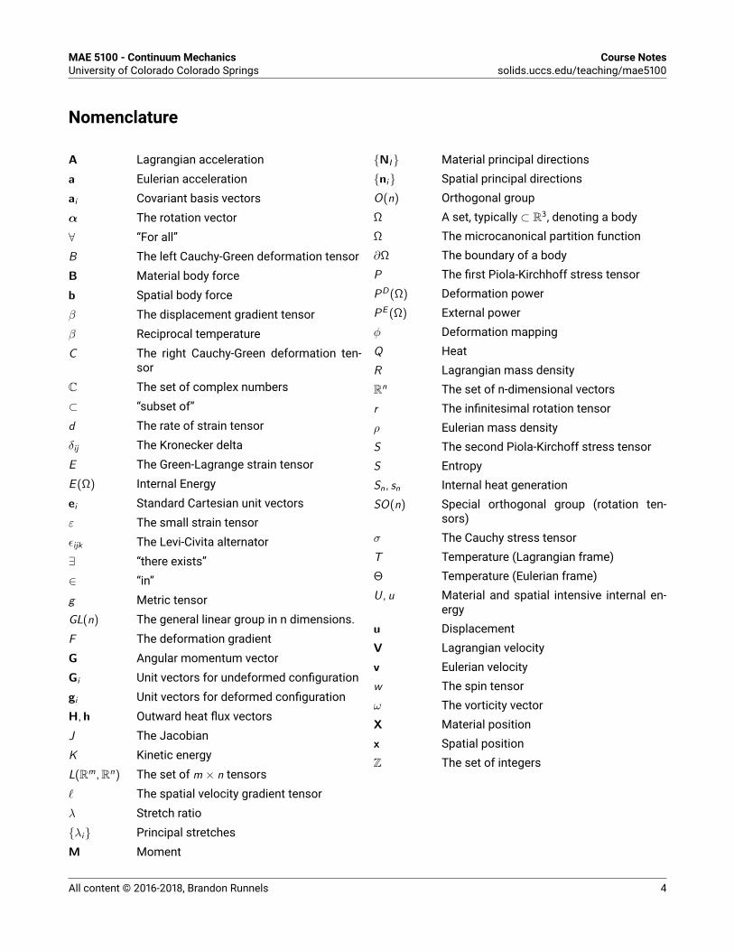
Nomenclature
A Lagrangian accelerationa Eulerian accelerationai Covariant basis vectorsα The rotation vector∀ “For all”B The left Cauchy-Green deformation tensorB Material body forceb Spatial body forceβ The displacement gradient tensorβ Reciprocal temperatureC The right Cauchy-Green deformation ten-sorC The set of complex numbers⊂ “subset of”d The rate of strain tensorδij The Kronecker deltaE The Green-Lagrange strain tensorE (Ω) Internal Energyei Standard Cartesian unit vectorsε The small strain tensorεijk The Levi-Civita alternator∃ “there exists”∈ “in”g Metric tensorGL(n) The general linear group in n dimensions.F The deformation gradientG Angular momentum vectorGi Unit vectors for undeformed configurationgi Unit vectors for deformed configurationH,h Outward heat flux vectorsJ The JacobianK Kinetic energyL(Rm,Rn) The set of m × n tensors` The spatial velocity gradient tensorλ Stretch ratioλi Principal stretchesM Moment
NI Material principal directionsni Spatial principal directionsO(n) Orthogonal groupΩ A set, typically ⊂ R3, denoting a bodyΩ The microcanonical partition function∂Ω The boundary of a bodyP The first Piola-Kirchhoff stress tensorPD(Ω) Deformation powerPE (Ω) External powerφ Deformation mappingQ HeatR Lagrangian mass densityRn The set of n-dimensional vectorsr The infinitesimal rotation tensorρ Eulerian mass densityS The second Piola-Kirchoff stress tensorS EntropySn, sn Internal heat generationSO(n) Special orthogonal group (rotation ten-sors)σ The Cauchy stress tensorT Temperature (Lagrangian frame)Θ Temperature (Eulerian frame)U, u Material and spatial intensive internal en-ergyu DisplacementV Lagrangian velocityv Eulerian velocityw The spin tensorω The vorticity vectorX Material positionx Spatial positionZ The set of integers
All content © 2016-2018, Brandon Runnels 4
Lecture 1 Introduction and index notation
0 IntroductionWelcome to continuum mechanics. In this course we will develop the mathematical framework for describingprecisely the deformation of solids, fluids, and gasses, and describing the physical laws that govern their motion.We will develop the mathematical formulation of the equations of motion, elasticity, viscoelasticity, plasticity, etc.The course will be organized in the following way:(1) Tensor analysis: index notation, tensor algebra and calculus, curvilinear coordinates and transformationrules.(2) Kinematics of deformation: deformation mappings, local deformation, metric changes, decompositions,compatibility, linearized kinematics.(3) Balance laws: conservation of mass, linear momentum, angular momentum, energy.(4) Constitutive modeling and the thermodynamics of solids: constitutive models, second law of thermodynam-ics and dissipative systems.(5) Computational mechanics: finite elements, Galerkin method, Ritz method.
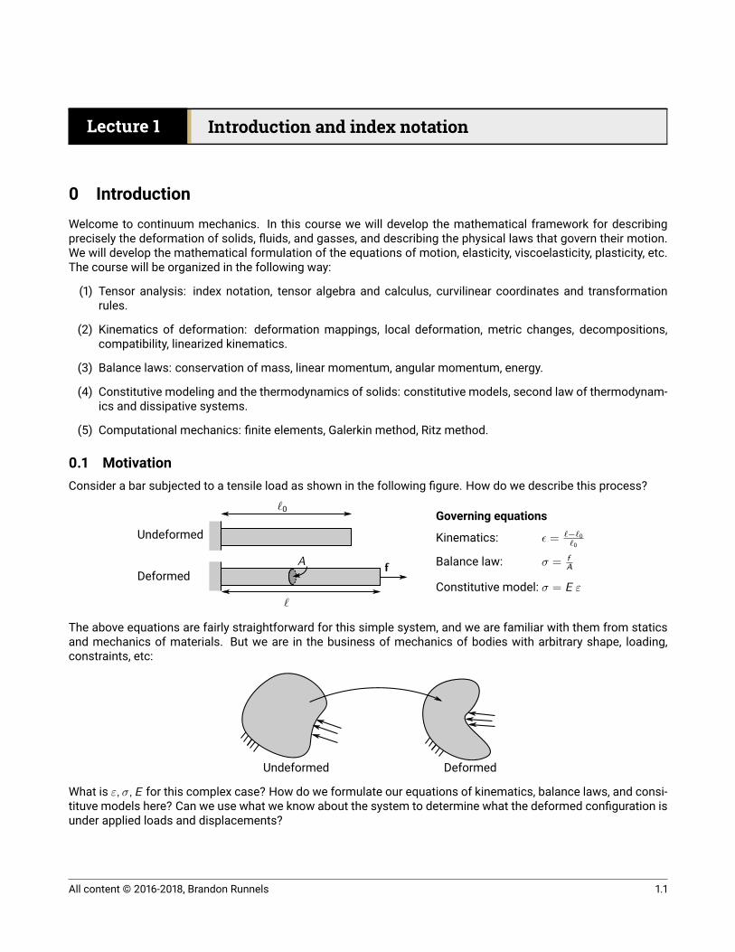
0.1 MotivationConsider a bar subjected to a tensile load as shown in the following figure. How do we describe this process?
f
`0
`
A
ε = `−`0
`0
σ = fA
σ = E ε
Kinematics:Balance law:Constitutive model:
Governing equationsUndeformed
Deformed
The above equations are fairly straightforward for this simple system, and we are familiar with them from staticsand mechanics of materials. But we are in the business of mechanics of bodies with arbitrary shape, loading,constraints, etc:
Undeformed DeformedWhat is ε,σ,E for this complex case? How do we formulate our equations of kinematics, balance laws, and consi-tituve models here? Can we use what we know about the system to determine what the deformed configuration isunder applied loads and displacements?
All content © 2016-2018, Brandon Runnels 1.1
MAE 5100 - Continuum MechanicsUniversity of Colorado Colorado Springs Course Notes - Lecture 1solids.uccs.edu/teaching/mae5100
0.2 NotationContinuummechanics is built on the mathematical framework of differential geometry. As a result, the conventionis to use standardmath notationwhen formulating continuummechanics. Additionally, aswewill see, it is generallynecessary to maintain a level of mathematical precision beyond that typically found in engineering disciplines.0.2.1 Sets
A set is a collection of objects. Examples:• The integers Z = ... ,−1, 0, 1, 2, 3, ...
• The real numbers R
• The complex numbers C
• n-dimensional vectors Rn
To indicate that an item is in a set, we use the ∈ symbol. For instance,x ∈ R3 (0.1)
indicates that x is a 3D vector. To indicate that a set is a subset, we use the ⊂ symbol. For instanceZ ⊂ R (0.2)
indicates that the integers are a subset of the real numbers. Another common use is to denote a 3D body:Ω ⊂ R3 (0.3)
is an arbitrary region in 3D space.0.2.2 Proof notation
We will not be doing any serious proofs in this course, but we frequently use some of the proof notation to simplifydefinitions and theorems.• ∃ is read “there exists.” For instance, ∃x ∈ R3 states that there is at least one item in the R3 set, or that the R3
set is not empty.• ∀ is read “for all.” For instance,
x− x = 0 ∀x ∈ Rn (0.4)tells us that the statement x− x = 0 is true for every possible vector.
Example:∀x ∈ R3 ∃a ∈ R3 s.t. x− a = 0 (0.5)
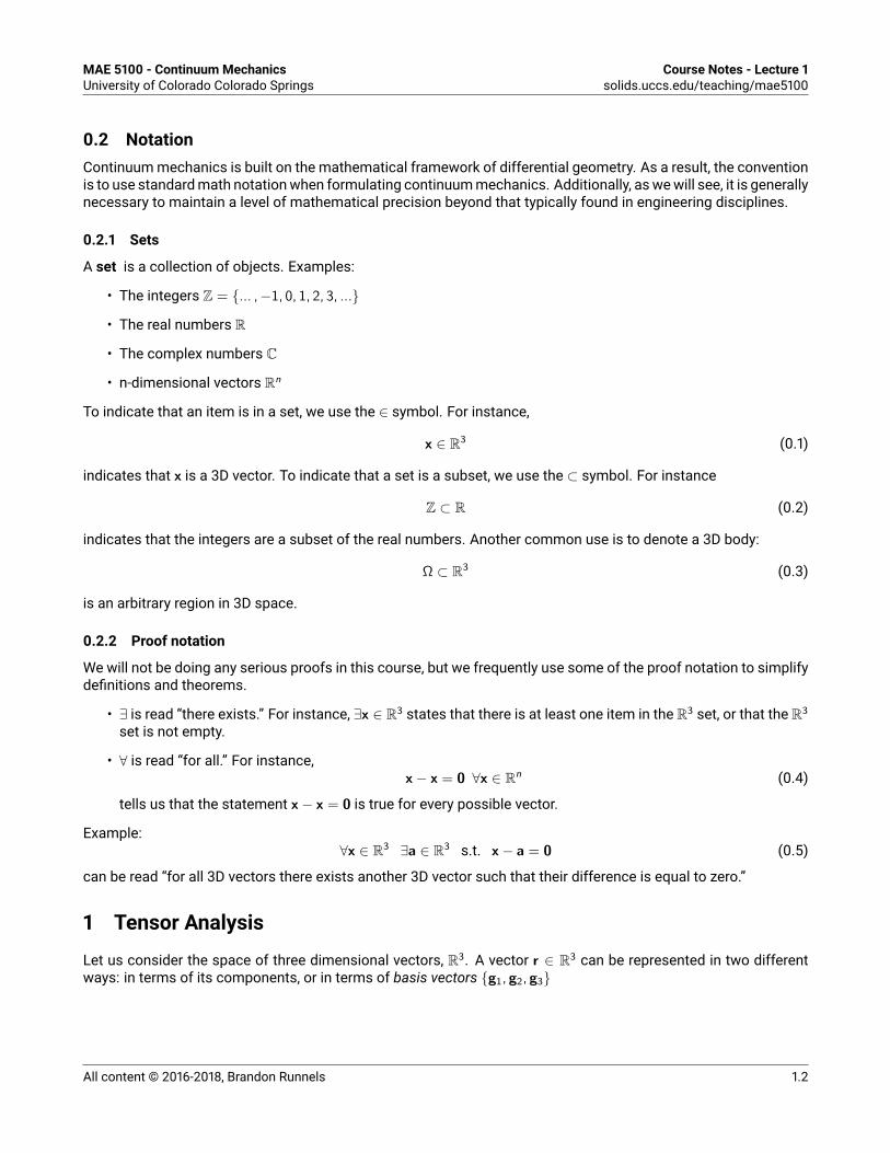
can be read “for all 3D vectors there exists another 3D vector such that their difference is equal to zero.”1 Tensor AnalysisLet us consider the space of three dimensional vectors, R3. A vector r ∈ R3 can be represented in two differentways: in terms of its components, or in terms of basis vectors g1, g2, g3
All content © 2016-2018, Brandon Runnels 1.2
MAE 5100 - Continuum MechanicsUniversity of Colorado Colorado Springs Course Notes - Lecture 1solids.uccs.edu/teaching/mae5100
g1x
y
z
a b
c
g2
g3
r =
[abc
]r = r1g1 + r2g2 + r3g3
For example, we may haveg1 =
[100
]g2 =
[010
]g3 =
[001
](1.1)
where we see that the basis vectors correspond to the familiar i, j, k notation. For maximum generality, however,we do not define the basis vectors explicitly. In subsequent sections will talk about changes of basis.Note also that we have dropped the familiar x , y , z notation in favor of 1, 2, 3. In general, we will stick with thisconvention exclusively; the reason for this will become apparent in the next section.1.1 Index notation and the Einstein summation conventionLet us consider r defined in the previous section as
r = r1 g1 + r2 g2 + r3 g3 (1.2)We can write this more simply using summation notation:
r =3∑
i=1
ri gi (1.3)It turns out that we write sums like this a lot, and it becomes cumbersome to write the summation symbol everytime. Thus, we introduce the Einstein summation convention, and we drop the explicit sum. This allows us to simplywrite
r = ri gi (1.4)This leads us to define the rules of the summation convention. For a vector equation in Rn , expressed using indexnotation:Rule 1: An index appearing once in a term must appear in every term in the equation, and is not summed. Itis referred to as a free index.Rule 2: An index appearing twice must be summed from 1 to n. It is referred to as a dummy index.(Dummy indices can be changed arbitrarily, that is, e.g. rigi = rjgj )Rule 3: No index may appear more than twice in any term.(If an index does appear more than twice, we go back to using a summation symbol. Alternatively, ifan index appears twice but is not a dummy index, we use parentheses to denote this, e.g. ui = λ(i) v(i).Fortunately, these cases are pretty rare. Usually, when a rule gets broken, it means that some algebragot messed up.)These rules may seem a bit strange, and they usually take a little bit of time to get used to. To help solidify them,let us look at a couple of algebraic examples.(Fun fact: the Einstein summation conventionwas introduced by Albert Einstein to simplify the equations of generalrelativity. In fact, the formulation of continuum mechanics has a number of similarities to general relativity.)All content © 2016-2018, Brandon Runnels 1.3
MAE 5100 - Continuum MechanicsUniversity of Colorado Colorado Springs Course Notes - Lecture 1solids.uccs.edu/teaching/mae5100
1.1.1 Vector equality
Consider two vectors u, v ∈ Rn with components u1, u2, ..., v1, v2, .... In invariant/symbolic notation, we say the twovectors are equal ifu = v or ui gi = vi gi (1.5)
This tells us that each component of the vector is equal; in other words,ui = vi (1.6)
Does this obey the summation convention? Yes it does: i is a free index that appears exactly once in every term ofthe equation.1.1.2 Inner product
Let us again consider u, v ∈ Rn. The inner product (or “dot product”) is defined asu · v = uTv = ||u|| ||v|| cos θ (1.7)
where || · || is the magnitude of · and θ is the angle between the two vectors. In matrix notation, we evaluate this asuTv = [u1 u2 ... un]
v1v2...vn
= u1v1 + u2v2 + ... + unvn =n∑
i=1
uivi = uivi (1.8)Note that there are no free indices, only dummy indices.1.1.3 Kronecker delta
The Kronecker Delta is defined in the following way:δij =
1 i = j
0 i 6= j(1.9)
Consider the basis vectors that we described above. We know that they are orthonormal, so gi · gj is 1 if i = j and0 otherwise; that is,
gi · gj = δij (1.10)Let us use this technology in the context of the dot product. Let u = ui gi , v = vi gi . Then we might write the dotproduct as
u · v = (ui gi ) · (vi gi ) (1.11)But wait: this breaks one of our rules, that an index cannot repeat more than twice. To fix this, we will replace theis in the second term with js:
u · v = (ui gi ) · (vj gj) (1.12)Now, let us distribute these terms:
u · v = ui vj (gi · gj) = ui vj δij (1.13)This term has two summed indices, so if we expand it out, we would have n2 terms. However, we know that onlythe terms where i = j survive. Thus, the effect of the Kronecker Delta is to turn one of the dummy indices into theother: in this case, if we “sum over j”
ui vj δij = ui vi (1.14)All content © 2016-2018, Brandon Runnels 1.4
MAE 5100 - Continuum MechanicsUniversity of Colorado Colorado Springs Course Notes - Lecture 1solids.uccs.edu/teaching/mae5100
1.1.4 Components of a vector
To extract a specific component of a vector, we can dot with the corresponding unit vector. That is:u · gi = (uj gj) · gi = uj (gi · gj) = uj δij = ui (1.15)
1.1.5 Norm of a vector
As you may recall, the norm of a vector is given by||u|| =
√u · u (1.16)
In index notation, this becomes||u|| =
√ui ui (1.17)
1.1.6 Permutation tensor
The next order of business is to introduce the cross product in tensor notation. To work with cross products, weneed to introduce a new bit of machinery, called the permutation tensor, also referred to as the Levi-Civita tensor.(Note: it’s not actually a tensor. However, it is frequently referred to as one, so we will stick with convention here.)Here it is:εijk =
1 ijk = 123, 231, 312 = "even permutation"−1 ijk = 321, 132, 213 = "odd permutation"0 otherwise
(1.18)
Let’s make a couple of notes here:• εijk is zero if any of the two indices take the same value.• Flipping two indices changes the sign of ε; that is, e.g.
εijk = −εjik = −εikj = −εkji (1.19)These identities will come in handy in the future.1.1.7 Cross product
Let us consider the cross product of unit vectors. We know thatg1 × g2 = g3 g2 × g1 = −g3 (1.20)g2 × g3 = g1 g3 × g2 = −g1 (1.21)g3 × g1 = g2 g1 × g3 = −g2 (1.22)
Let us attempt to express this using the permutation tensor. Try:gi × gj = εijkgk (1.23)
Does this work? Let’s plug in i = 1, j = 2. Then we haveg1 × g2 = ε12kgk =:
0ε121g1 +:0ε122g2 + ε123g3 = g3 (1.24)
as expected. Plugging in other values for i , j shows that we can recover all of the identities expressed above. Now,let us see what happens when we take the cross product between u, v:u× v = (ui gi )× (vj gj) = ui vj (gi × gj) = ui vi εijk gk (1.25)
Alternatively,(u× v)k = εijk ui vj (1.26)
All content © 2016-2018, Brandon Runnels 1.5
MAE 5100 - Continuum MechanicsUniversity of Colorado Colorado Springs Course Notes - Lecture 1solids.uccs.edu/teaching/mae5100
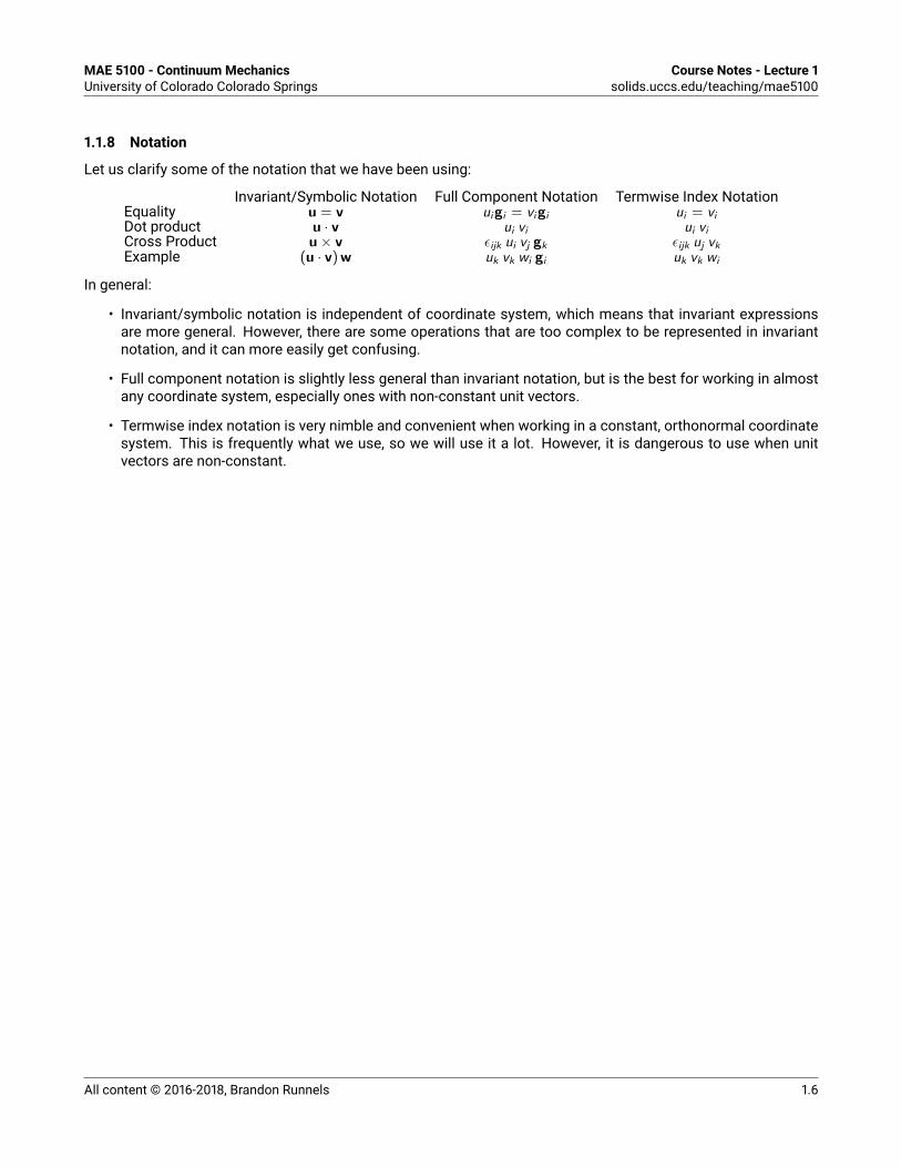
1.1.8 Notation
Let us clarify some of the notation that we have been using:Invariant/Symbolic Notation Full Component Notation Termwise Index NotationEquality u = v uigi = vigi ui = viDot product u · v ui vi ui viCross Product u× v εijk ui vj gk εijk uj vkExample (u · v)w uk vk wi gi uk vk wi
In general:• Invariant/symbolic notation is independent of coordinate system, which means that invariant expressionsare more general. However, there are some operations that are too complex to be represented in invariantnotation, and it can more easily get confusing.• Full component notation is slightly less general than invariant notation, but is the best for working in almostany coordinate system, especially ones with non-constant unit vectors.• Termwise index notation is very nimble and convenient when working in a constant, orthonormal coordinatesystem. This is frequently what we use, so we will use it a lot. However, it is dangerous to use when unitvectors are non-constant.
All content © 2016-2018, Brandon Runnels 1.6

Lecture 2 Mappings and tensors
1.2 Mappings and tensorsA mapping is a machine that takes a thing of one type and turns it into a thing of another type. For instance,f (x) = x2 takes a real number and turns it into a positive real number. We use the notation
f : U → V (1.27)to denote a mapping; in this case, if x ∈ U , then f (x) ∈ V .A linear mapping f : Rn → Rm is a mapping that satisfies
• f (α x) = α f (x) ∀ x ∈ Rn, α ∈ R
• f (x + y) = f (x) + f (y) ∀ x, y ∈ Rn
1.2.1 Second order tensors
A second order tensor (S.O.T.) is a linear mapping from vector spaces to vector spaces. The set of second ordertensors mapping n-dimensional vectors to m-dimensional vectors is referred to as L(Rn,Rn). We are familiar withthinking of them as n ×m matrices: For example, if A ∈ L(Rn,Rm) and u ∈ Rn, v ∈ Rm then we could write
v = Au
v1v2...vm
=
A11 A12 ... A1nA21 A22 ... A2n... ... . . . ...Am1 Am2 ... Amn
u1u2...un
(1.28)
We can write all possible linear mappings from Rn to Rm in matrix form. Therefore, in general, we can think ofsecond order tensors as being similar to matrices. Let us make a few notes:• If m = n the matrix is said to be square. For the most part, we will work with square matrices.• If u = Au then A = I is said to be the identity mapping.• The difference between tensors and matrices is subtle. A matrix is just a collection of numbers, but a ten-sor is something that must be transformed with a change of coordinates. Thus we say that tensors havetransformation properties but matrices do not.
1.2.2 Index notation
Index notationmakes it very convenient towrite second order tensors and tensor-vectormultiplication. In the aboveexample, we have v1v2...vm
=
A11u1 + A12u2 + ... + A1nunA21u1 + A22u2 + ... + A2nun...Am1u1 + Am2u2 + ... + Amnun
(1.29)
and so we can writevi = Aijuj (1.30)
All content © 2016-2018, Brandon Runnels 2.1
MAE 5100 - Continuum MechanicsUniversity of Colorado Colorado Springs Course Notes - Lecture 2solids.uccs.edu/teaching/mae5100
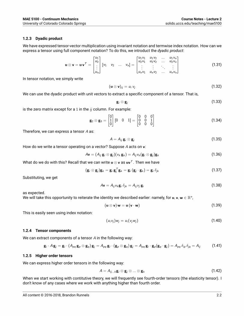
1.2.3 Dyadic product
We have expressed tensor-vector multiplication using invariant notation and termwise index notation. How can weexpress a tensor using full component notation? To do this, we introduct the dyadic product:
u⊗ v = u vT =
u1u2...un
[v1 v2 ... vn] =
u1v1 u1v2 ... u1vnu2v1 u2v2 ... u2vn... ... . . . ...unv1 unv2 ... unvn
(1.31)
In tensor notation, we simply write(u⊗ v)ij = ui vj (1.32)
We can use the dyadic product with unit vectors to extract a specific component of a tensor. That is,gi ⊗ gj (1.33)
is the zero matrix except for a 1 in the ij column. For example:g2 ⊗ g3 =
[010
][0 0 1] =
[0 0 00 0 10 0 0
](1.34)
Therefore, we can express a tensor A as:A = Aij gi ⊗ gj (1.35)
How do we write a tensor operating on a vector? Suppose A acts on v:Av = (Aij gi ⊗ gj)(vk gk) = Aijvk(gi ⊗ gj)gk (1.36)
What do we do with this? Recall that we can write u⊗ v as uvT . Then we have(gi ⊗ gj)gk = gi g
Tj gk = gi (gj · gk) = gi δjk (1.37)
Substituting, we getAv = Aijvkgi δjk = Aijvj gi (1.38)
as expected.We will take this opportunity to reiterate the identity we described earlier: namely, for u, v,w ∈ Rn ,(u⊗ v)w = u (v ·w) (1.39)
This is easily seen using index notation:(uivj)wj = ui (vjwj) (1.40)
1.2.4 Tensor components
We can extract components of a tensor A in the following way:gi · A gj = gi · (Apq gp ⊗ gq) gj = Apq gi · (gp ⊗ gq) gj = Apq gi · gp(gq · gj) = Apq δip δjq = Aij (1.41)
1.2.5 Higher order tensors
We can express higher order tensors in the following way:A = Aij ...kgi ⊗ gj ⊗ ...⊗ gk (1.42)
When we start working with contitutive theory, we will frequently see fourth-order tensors (the elasticity tensor). Idon’t know of any cases where we work with anything higher than fourth order.All content © 2016-2018, Brandon Runnels 2.2
MAE 5100 - Continuum MechanicsUniversity of Colorado Colorado Springs Course Notes - Lecture 2solids.uccs.edu/teaching/mae5100
1.2.6 Transpose
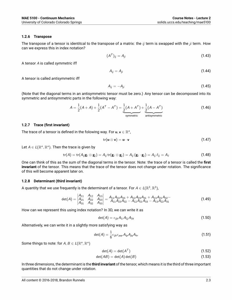
The transpose of a tensor is identitcal to the transpose of a matrix: the ij term is swapped with the ji term. Howcan we express this in index notation?(AT )ij = Aji (1.43)
A tensor A is called symmetric iffAij = Aji (1.44)
A tensor is called antisymmetric iffAij = −Aji (1.45)
(Note that the diagonal terms in an antisymmetric tensor must be zero.) Any tensor can be decomposed into itssymmetric and antisymmetric parts in the following way:A =
1
2(A + A) +
1
2(AT − AT ) =
1
2(A + AT )︸ ︷︷ ︸symmetric
+1
2(A− AT )︸ ︷︷ ︸
antisymmetric(1.46)
1.2.7 Trace (first invariant)
The trace of a tensor is defined in the folowing way. For u, v ∈ Rn ,tr(u⊗ v) = u · v (1.47)
Let A ∈ L(Rn,Rn). Then the trace is given bytr(A) = tr(Aijgi ⊗ gj) = Aij tr(gi ⊗ gj) = Aij (gi · gj) = Aij δij = Aii (1.48)
One can think of this as the sum of the diagonal terms in the tensor. Note: the trace of a tensor is called the firstinvariant of the tensor. This means that the trace of the tensor does not change under rotation. The significanceof this will become apparent later on.1.2.8 Determinant (third invariant)
A quantity that we use frequently is the determinant of a tensor. For A ∈ L(R3,R3),det(A) =
∣∣∣∣∣A11 A12 A13A21 A22 A23A31 A32 A33
∣∣∣∣∣ =A11A22A33 + A12A23A31 + A13A21A32−A11A23A32 − A12A21A33 − A13A22A31
(1.49)How can we represent this using index notation? In 3D, we can write it as
det(A) = εijkA1iA2jA3k (1.50)Alternatively, we can write it in a slightly more satisfying way as
det(A) =1
6εijkεpqrAipAjqAkr (1.51)
Some things to note: for A,B ∈ L(Rn,Rn)
det(A) = det(AT ) (1.52)det(AB) = det(A) det(B) (1.53)
In three dimensions, the determinant is the third invariantof the tensor, whichmeans it is the third of three importantquantities that do not change under rotation.All content © 2016-2018, Brandon Runnels 2.3
MAE 5100 - Continuum MechanicsUniversity of Colorado Colorado Springs Course Notes - Lecture 2solids.uccs.edu/teaching/mae5100
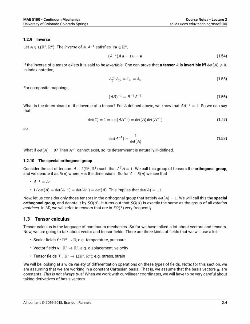
1.2.9 Inverse
Let A ∈ L(Rn,Rn). The inverse of A, A−1 satisfies, ∀u ∈ Rn ,(A−1)Au = Iu = u (1.54)
If the inverse of a tensor exists it is said to be invertible. One can prove that a tensor A is invertible iff det(A) 6= 0.In index notation,A−1ij Ajk = Iik = δik (1.55)
For composite mappings,(AB)−1 = B−1A−1 (1.56)
What is the determinant of the inverse of a tensor? For A defined above, we know that AA−1 = I. So we can saythatdet(I) = 1 = det(AA−1) = det(A) det(A−1) (1.57)
sodet(A−1) =
1
det(A)(1.58)
What if det(A) = 0? Then A−1 cannot exist, so its determinant is naturally ill-defined.1.2.10 The special orthogonal group
Consider the set of tensors A ∈ L(R3,R3) such that ATA = I. We call this group of tensors the orthogonal group,and we denote it as S(n) where n is the dimensions. So for A ∈ S(n) we see that• A−1 = AT
• 1/ det(A) = det(A−1) = det(AT ) = det(A). This implies that det(A) = ±1
Now, let us consider only those tensors in the orthogonal group that satisfy det(A) = 1. We will call this the specialorthogonal group, and denote it by SO(d). It turns out that SO(d) is exactly the same as the group of all rotationmatrices. In 3D, we will refer to tensors that are in SO(3) very frequently.1.3 Tensor calculusTensor calculus is the language of continuum mechanics. So far we have talked a lot about vectors and tensors.Now, we are going to talk about vector and tensor fields. There are three kinds of fields that we will use a lot:
• Scalar fields f : Rn → R; e.g. temperature, pressure• Vector fields v : Rn → Rn; e.g. displacement, velocity• Tensor fields T : Rn → L(Rn,Rn); e.g. stress, strain
We will be looking at a wide variety of differentiation operations on these types of fields. Note: for this section, weare assuming that we are working in a constant Cartesian basis. That is, we assume that the basis vectors gi areconstants. This is not always true! When we work with curvilinear coordinates, we will have to be very careful abouttaking derivatives of basis vectors.
All content © 2016-2018, Brandon Runnels 2.4
MAE 5100 - Continuum MechanicsUniversity of Colorado Colorado Springs Course Notes - Lecture 2solids.uccs.edu/teaching/mae5100
1.3.1 Gradient
Suppose we have a scalar field φ : Rn → R, φ(x). We define the gradient of φ to begrad(φ) =
∂φ
∂x1g1 +
∂φ
∂x2g2 + ... +
∂φ
∂xngn =
∂φ
∂xigi (1.59)
Note that gradient operator turns a scalar field into a vector field.Now consider a vector field u : Rn → Rn. The gradient of u is defined to begrad(u) =
∂u
∂xi⊗ gi =
∂ui∂xj
gi ⊗ gj (1.60)Note that the gradient operator here turns a vector field into a tensor field.We can generalize this in the following way:
grad(·) =∂(·)∂xi⊗ gi (1.61)
where we drop the dyadic product if · is a scalar field. In general, we only generally care about gradients on scalarand vector fields. However, there are some models that depend on tensor field gradients, such as strain gradientplasticity and ductile fracture.
All content © 2016-2018, Brandon Runnels 2.5
Lecture 3 Tensor calculus
1.3.2 Divergence
For a vector field u : Rn → Rn , the divergence is defined to bediv(u) =
∂u
∂xi· gi =
∂uj∂xi
gj · gi =∂uj∂xi
δij =∂ui∂xi
(1.62)Note that the divergence turns a vector field into a scalar field. Now, consider a tensor field T : Rn → L(Rn,Rn).The divergence of the tensor field is
div(T ) =dT
dxigi =
dTjk
dxi(gj ⊗ gk)gi =
dTjk
dxigj(gk · gi ) =
dTjk
dxigjδik =
dTji
dxigj (1.63)
Note that the divergence turns a tensor field into a vector field. We can generalize this in the same way we gener-alized the gradient:div(·) =
∂(·)∂xi· gi (1.64)
where we drop the dot for tensor fields. Note also that we cannot take the divergence of a scalar field.1.3.3 Laplacian
The Laplacian is the composition of the gradient and the divergence operators on a scalar field: for φ : R→ R:∆φ = div(grad(φ)) (1.65)
In Cartesian coordinates, this comes out to be∆φ =
∂2φ
∂xi∂xi(1.66)
Note that we do not write ∂x2i in order to be in keeping with the summation convention.
1.3.4 Curl
The curl operator is defined on a vector field u : R3 → R3 in the following way:curl(u) = − ∂u
∂xi× gi = −∂uj
∂xigj × gi = −∂uj
∂xiεjikgk =
∂uj∂xi
εijkgk (1.67)Note that the curl acts on a vector field and produces a vector field, so we cannot take the curl of a scalar field. Ingeneralized form we have
curl(·) = −∂(·)∂xi× gi (1.68)
1.3.5 Gateaux derivatives
A more general type of derivative is the “Gateaux derivative,” which will prove very useful later on. Consider somefield (scalar, vector, or tensor, etc.) φ : Rn → V (where V is the set of scalars, vectors, tensors, etc.) and a vectorv ∈ Rn. The Gateaux derivative is defined as
Dφ(x)v =d
dεφ(x + εv)
∣∣∣∣ε→0
(1.69)that is, the derivative is taken with respect to ε which is then set to 0.All content © 2016-2018, Brandon Runnels 3.1
MAE 5100 - Continuum MechanicsUniversity of Colorado Colorado Springs Course Notes - Lecture 3solids.uccs.edu/teaching/mae5100
Example 1.1
Let φ(x) = xixi = ||x||2, and compute Dφ(x)v. We evaluate this simply by substituting φ into (1.69):Dφ(x)v = lim
ε→0
d
dε((xi + εvi )(xi + εvi )) = lim
ε→0
d
dε(xixi + 2εxivi + ε2vivi ) = lim
ε→0(2xivi + 2εvivi ) = 2xivi (1.70)
1.3.6 Notation
Here it is important to make a couple of remarks about notation.(1) We avoid the use of the ∇ operator (e.g. ∇· for divergence, ∇× for curl) because it is difficult to impossibleto express certain vector operations.(2) We work with a lot of derivatives in continuum mechanics and it frequently becomes cumbersome to write
∂∂xi
. Therefore, we adopt comma notation:∂
∂xi(·) = (·),i (1.71)
For example, we can write grad/div/curl compactly for scalar/vector/tensor fields φ, v,T
grad(φ)i = φ,i div(v) = vi ,i curl(v)i = εijkvk,j ∆φ = φ,ii (1.72)grad(v)ij = vi ,j div(T )i = Tij ,j (1.73)
(3) We will occasionally use the ∂ symbol to denote differentiation. Examples of usage include:∂x ≡
∂
∂x∂θ ≡
∂
∂θ∂i ≡
∂
∂xi(1.74)
1.3.7 Evaluating derivatives
How do we evaluate a derivative with respect to x in terms of x? For instance, how would we compute the gradientof φ(x) = x · x?In index notation, we have∂xi∂xj
= δij or, in symbolic notation, ∂x
∂x= I (1.75)
Let us look at a couple of examples:Example 1.2
Compute the gradient of φ(x) = x · x. The first step is to write φ in index notation: φ(x) = xkxk . Then, we usethe formula:grad(φ) =
∂
∂xi(xkxk) gi (1.76)
We can use the product rule exactly like we would normally:= (δikxk + xkδik) gi = 2δikxk gi (1.77)
Summing over i we get= 2xi gi = 2x (1.78)
All content © 2016-2018, Brandon Runnels 3.2
MAE 5100 - Continuum MechanicsUniversity of Colorado Colorado Springs Course Notes - Lecture 3solids.uccs.edu/teaching/mae5100
Example 1.3
Let φ : R3 → R. Show that Dφ(x)v = grad(φ) · v. To do this we again evaluate the Gateaux derivative:Dφ(x)v = lim
ε→0
d
dεφ(x + ε v) (1.79)
We use the chain rule exactly as we would normally:= limε→0
∂φ(x + ε v)
∂(xi + ε xi )
d(xi + ε vi )
dε= limε→0
∂φ(x + ε v)
∂(xi + ε xi )vi =
∂φ
∂xivi = grad(φ) · v (1.80)
In addition to taking derivatives with respect to vectors (such as x) wemay take derivatives with respect to tensors.For example, given φ : L(Rn,Rn)→ R, we may wish to calculatedφ(T )
dTij(1.81)
Similarly to the case of vectors, we havedTij
dTpq= δipδjq or, in symbolic notation, dT
dT= I⊗ I (1.82)
Example 1.4
Let A : L(Rn,Rn)→ L(Rn,Rn) with A(T ) = TTT . Find the derivative of A with respect to T :∂Aij
∂Tpq=
∂
∂Tpq(TkiTkj) =
∂Tki
∂TpqTkj + Tki
∂Tkj
∂Tpq= δkpδiqTkj + Tkiδkpδjq = Tpjδiq + Tpiδjq (1.83)
How do we represent this in symbolic notation? It’s actually rather tricky, and is much easier to leave thingsin index notation.Note: when taking vector or tensor derivatives, it is always important to use a fresh new free index. Do not reuseexisting ones.1.4 The divergence theoremWe have developed enoughmachinery to introduce the singlemost important theorem in all of continuummechan-ics: the divergence theorem.
V(x)
n
Ω
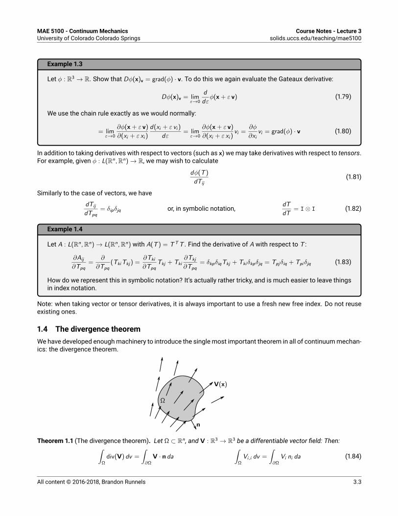
Theorem 1.1 (The divergence theorem). Let Ω ⊂ Rn , and V : R3 → R3 be a differentiable vector field: Then:∫Ω
div(V) dv =
∫∂Ω
V · n da∫
Ω
Vi ,i dv =
∫∂Ω
Vi ni da (1.84)
All content © 2016-2018, Brandon Runnels 3.3
MAE 5100 - Continuum MechanicsUniversity of Colorado Colorado Springs Course Notes - Lecture 3solids.uccs.edu/teaching/mae5100
where ∂Ω is the boundary of the body.
We have a similar theorem for tensor fields: Let T : R3 → L(R3,R3) be a tensor field. Then∫Ω
div(T ) dv =
∫∂Ω
Tn da (1.85)Using index notation in an Cartesian coordinate system, we can write∫
Ω
Vi ,i dv =
∫∂Ω
Vi ni da
∫Ω
Tij ,j dv =
∫∂Ω
Tij nj da (1.86)What does this mean? We are relating a volume integral of the divergence to a surface integral – or, in this case, aflux integral. For the case of a vector field, the integral of the divergence over the body can be intuitively thoughtof as the total amount of compression/expansion in the vector field. The flux integral can be thought of as thetotal amount of vector field entering or leaving the body. Thus, you can think of the divergence theorem as themathematical formulation of the statement “the total compression of the vector field is equal to the rate of fluxthrough the boundary.” We will make extensive use of the divergence theorem in this course.
All content © 2016-2018, Brandon Runnels 3.4
Lecture 4 Curvilinear coordinates and tensor transformations
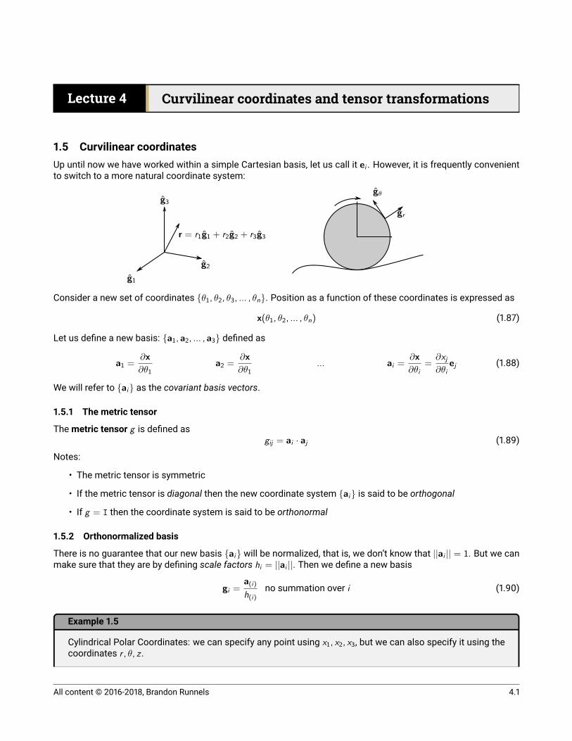
1.5 Curvilinear coordinatesUp until now we have worked within a simple Cartesian basis, let us call it ei . However, it is frequently convenientto switch to a more natural coordinate system:
g1
g2
g3
r = r1g1 + r2g2 + r3g3
gr
gθ
Consider a new set of coordinates θ1, θ2, θ3, ... , θn. Position as a function of these coordinates is expressed asx(θ1, θ2, ... , θn) (1.87)
Let us define a new basis: a1, a2, ... , a3 defined asa1 =
∂x
∂θ1a2 =
∂x
∂θ1... ai =
∂x
∂θi=∂xj∂θi
ej (1.88)We will refer to ai as the covariant basis vectors.1.5.1 The metric tensor
The metric tensor g is defined asgij = ai · aj (1.89)
Notes:• The metric tensor is symmetric• If the metric tensor is diagonal then the new coordinate system ai is said to be orthogonal
• If g = I then the coordinate system is said to be orthonormal
1.5.2 Orthonormalized basis
There is no guarantee that our new basis ai will be normalized, that is, we don’t know that ||ai || = 1. But we canmake sure that they are by defining scale factors hi = ||ai ||. Then we define a new basisgi =
a(i)
h(i)no summation over i (1.90)
Example 1.5
Cylindrical Polar Coordinates: we can specify any point using x1, x2, x3, but we can also specify it using thecoordinates r , θ, z .
All content © 2016-2018, Brandon Runnels 4.1
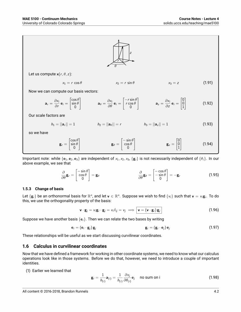
MAE 5100 - Continuum MechanicsUniversity of Colorado Colorado Springs Course Notes - Lecture 4solids.uccs.edu/teaching/mae5100
θ
r
z
Let us compute x(r , θ, z):x1 = r cos θ x2 = r sin θ x3 = z (1.91)
Now we can compute our basis vectors:ar =
∂xi∂r
ei =
[cos θsin θ
0
]aθ =
∂xi∂θ
ei =
[−r sin θr cos θ
0
]az =
∂xi∂z
ei =
[001
](1.92)
Our scale factors areh1 = ||ar || = 1 h2 = ||aθ|| = r h3 = ||az || = 1 (1.93)
so we havegr =
[cos θsin θ
0
]gθ =
[− sin θcos θ
0
]gz =
[001
](1.94)
Important note: while e1, e2, e3 are independent of x1, x2, x3, gi is not necessarily independent of θi. In ourabove example, we see that∂
∂θgr =
[− sin θcos θ
0
]= gθ
∂
∂θgθ =
[− cos θ− sin θ
0
]= −gr (1.95)
1.5.3 Change of basis
Let gi be an orthonormal basis for Rn , and let v ∈ Rn. Suppose we wish to find vi such that v = vigi . To dothis, we use the orthogonality property of the basis:v · gj = vigi · gj = viδij = vj =⇒ v = (v · gi ) gj (1.96)
Suppose we have another basis ei. Then we can relate the two bases by writingei = (ei · gj) gj gi = (gi · ej) ej (1.97)
These relationships will be useful as we start discussing curvilinear coordinates.1.6 Calculus in curvilinear coordinatesNow that we have defined a framework for working in other coordinate systems, we need to knowwhat our calculusoperations look like in those systems. Before we do that, however, we need to introduce a couple of importantidentities.(1) Earlier we learned that
gi =1
h(i)a(i) =
1
h(i)
∂xj∂θ(i)
ej no sum on i (1.98)
All content © 2016-2018, Brandon Runnels 4.2
MAE 5100 - Continuum MechanicsUniversity of Colorado Colorado Springs Course Notes - Lecture 4solids.uccs.edu/teaching/mae5100
Howcanweexpress ei in termsof gj? Todo this, we’ll pull a trick. Remember that gi formsanorthonormalbasis for Rn: that means that we can express any vector in terms of that basis. For instance, a vector v canbe written as v = vigi . How do we find vi? It’s nothing other than v · gi . So we can write
v = (v · gi ) gi (1.99)We can do exactly the same thing for our original basis vectors
ei = (ei · gj) gj =∑j
1
hj(ei · aj) gj =
∑j
1
hj(ei ·
∂xk∂θj
ek) gj =∑j
1
hj
∂xk∂θj
(ei · ek)︸ ︷︷ ︸δik
gj =∑j
1
hj
∂xi∂θj
gj (1.100)
(Note that we broke one of our summation convention rules. To compensate for this we drop the summationnotation and use an explicit sum.)(2) There is an important theorem called the inverse function theorem that states:[∂θ
∂x
]=[ ∂x∂θ
]−1
=⇒ ∂θ
∂x
∂x
∂θ= I or, in index notation, ∂θi
∂xk
∂xk∂θj
= δij (1.101)We will use both of these rules to derive expressions for the familiar divergence, gradient, and curl in curvilinearcoordinates.1.6.1 Gradient
We want to express the gradient as computed in the abovegrad(f (θ)) =
∂
∂xi(f (θ)) ei =
∂f
∂θj
∂θj∂xi
ei =∂f
∂θj
∂θj∂xi
(∑k
1
hk
∂xi∂θk
gk)
=∑k
1
hk
∂f
∂θj
∂θj∂xi
∂xi∂θk︸ ︷︷ ︸δjk
gk =∑k
1
hk
∂f
∂θkgk (1.102)
Notice how this is almost identical to our original expression for the gradient, except that xi, ei have beenreplaced with θi, gi. The only difference is the presence of the scale factors. Let’s solidify this with an example:Example 1.6
Let us continue with our example of cylindrical polar coordinates. Let f = f (r , θ, z). Then we have:grad(f ) =
1
hr
∂f
∂rgr +
1
hθ
∂f
∂θgθ +
1
hz
∂f
∂zgz =
∂f
∂rgr +
1
r
∂f
∂θgθ +
∂f
∂zgz (1.103)
1.6.2 Divergence
Let v = vi (θ) gi be a vector field that is defined exclusively using the θi, gi coordinate system. What is thedivergence of this vector field? We can follow the exact same procedure as when computing the gradient:div(v) =
∂
∂xi(v) · ei =
∂v
∂θj
∂θj∂xi· ei =
∂v
∂θj
∂θj∂xi·∑k
1
hk
∂xi∂θk
gk =∑k
1
hk
∂v
∂θj
∂θj∂xi︸︷︷︸Jji
∂xi∂θk︸︷︷︸J−1ik
·gk =∑k
1
hk
∂v
∂θjδjk · gk (1.104)
=∑k
1
hk
∂v
∂θk· gk (1.105)
All content © 2016-2018, Brandon Runnels 4.3
MAE 5100 - Continuum MechanicsUniversity of Colorado Colorado Springs Course Notes - Lecture 4solids.uccs.edu/teaching/mae5100
Notice again howwe arrive at an almost identical formula except that we include scale factors. Wemust alsomakeone very important note: how do we evaluate the following?∂
∂θk(v) =
∂
∂θk(vigi ) =
∂vi∂θk
gi + vi∂gi∂θk
(1.106)In Cartesian coordinates the basis vectors are constant so their derivatives vanish. However, this is not true inmost other curvilinear coordinates! To illustrate this, let’s do an example:
Example 1.7
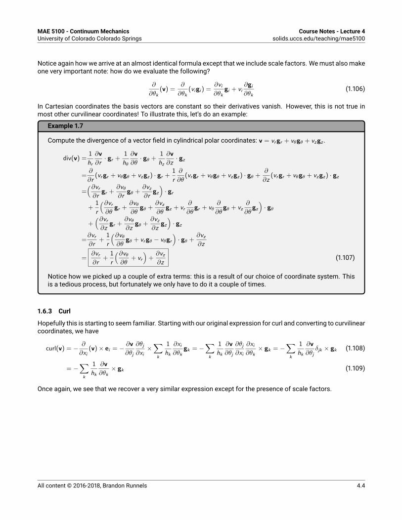
Compute the divergence of a vector field in cylindrical polar coordinates: v = vrgr + vθgθ + vzgz .div(v) =
1
hr
∂v
∂r· gr +
1
hθ
∂v
∂θ· gθ +
1
hz
∂v
∂z· gz
=∂
∂r(vrgr + vθgθ + vzgz) · gr +
1
r
∂
∂θ(vrgr + vθgθ + vzgz) · gθ +
∂
∂z(vrgr + vθgθ + vzgz) · gz
=(∂vr∂r
gr +∂vθ∂r
gθ +∂vz∂r
gz)· gr
+1
r
(∂vr∂θ
gr +∂vθ∂θ
gθ +∂vz∂θ
gz + vr∂
∂θgr + vθ
∂
∂θgθ + vz
∂
∂θgz)· gθ
+(∂vr∂z
gr +∂vθ∂z
gθ +∂vz∂z
gz)· gz
=∂vr∂r
+1
r
(∂vθ∂θ
gθ + vrgθ − vθgr)· gθ +
∂vz∂z
=∂vr∂r
+1
r
(∂vθ∂θ
+ vr)
+∂vz∂z
(1.107)Notice how we picked up a couple of extra terms: this is a result of our choice of coordinate system. Thisis a tedious process, but fortunately we only have to do it a couple of times.
1.6.3 Curl
Hopefully this is starting to seem familiar. Starting with our original expression for curl and converting to curvilinearcoordinates, we havecurl(v) = − ∂
∂xi(v)× ei = − ∂v
∂θj
∂θj∂xi×∑k
1
hk
∂xi∂θk
gk = −∑k
1
hk
∂v
∂θj
∂θj∂xi
∂xi∂θk× gk = −
∑k
1
hk
∂v
∂θjδjk × gk (1.108)
= −∑k
1
hk
∂v
∂θk× gk (1.109)
Once again, we see that we recover a very similar expression except for the presence of scale factors.
All content © 2016-2018, Brandon Runnels 4.4
MAE 5100 - Continuum MechanicsUniversity of Colorado Colorado Springs Course Notes - Lecture 4solids.uccs.edu/teaching/mae5100
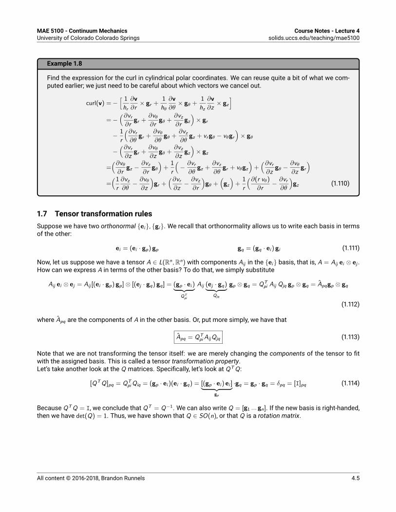
Example 1.8
Find the expression for the curl in cylindrical polar coordinates. We can reuse quite a bit of what we com-puted earlier; we just need to be careful about which vectors we cancel out.curl(v) =−
[ 1
hr
∂v
∂r× gr +
1
hθ
∂v
∂θ× gθ +
1
hz
∂v
∂z× gz
]=−
(∂vr∂r
gr +∂vθ∂r
gθ +∂vz∂r
gz)× gr
− 1
r
(∂vr∂θ
gr +∂vθ∂θ
gθ +∂vz∂θ
gz + vrgθ − vθgr)× gθ
−(∂vr∂z
gr +∂vθ∂z
gθ +∂vz∂z
gz)× gz
=(∂vθ∂r
gz −∂vz∂r
gθ)
+1
r
(− ∂vr∂θ
gz +∂vz∂θ
gr + vθgz)
+(∂vr∂z
gθ −∂vθ∂z
gr)
=(1
r
∂vz∂θ− ∂vθ
∂z
)gr +
(∂vr∂z− ∂vz
∂r
)gθ +
(gz)
+1
r
(∂(r vθ)
∂r− ∂vr∂θ
)gz (1.110)
1.7 Tensor transformation rulesSuppose we have two orthonormal ei, gi. We recall that orthonormality allows us to write each basis in termsof the other:
ei = (ei · gp) gp gq = (gq · ei ) gi (1.111)Now, let us suppose we have a tensor A ∈ L(Rn,Rn) with components Aij in the ei basis, that is, A = Aij ei ⊗ ej .How can we express A in terms of the other basis? To do that, we simply substitute
Aij ei ⊗ ej = Aij [(ei · gp) gp]⊗ [(ej · gq) gq] = (gp · ei )︸ ︷︷ ︸QT
pi
Aij (ej · gq)︸ ︷︷ ︸Qjq
gp ⊗ gq = QTpi Aij Qjq gp ⊗ gq = Apqgp ⊗ gq
(1.112)where Apq are the components of A in the other basis. Or, put more simply, we have that
Apq = QTpiAijQjq (1.113)
Note that we are not transforming the tensor itself: we are merely changing the components of the tensor to fitwith the assigned basis. This is called a tensor transformation property.Let’s take another look at the Q matrices. Specifically, let’s look at QTQ :[QTQ]pq = QT
piQiq = (gp · ei )(ei · gq) = [(gp · ei ) ei ]︸ ︷︷ ︸gp
·gq = gp · gq = δpq = [I]pq (1.114)
Because QTQ = I, we conclude that QT = Q−1. We can also write Q = [g1 ... gn]. If the new basis is right-handed,then we have det(Q) = 1. Thus, we have shown that Q ∈ SO(n), or that Q is a rotation matrix.
All content © 2016-2018, Brandon Runnels 4.5
Lecture 5 Kinematics of deformation, frames
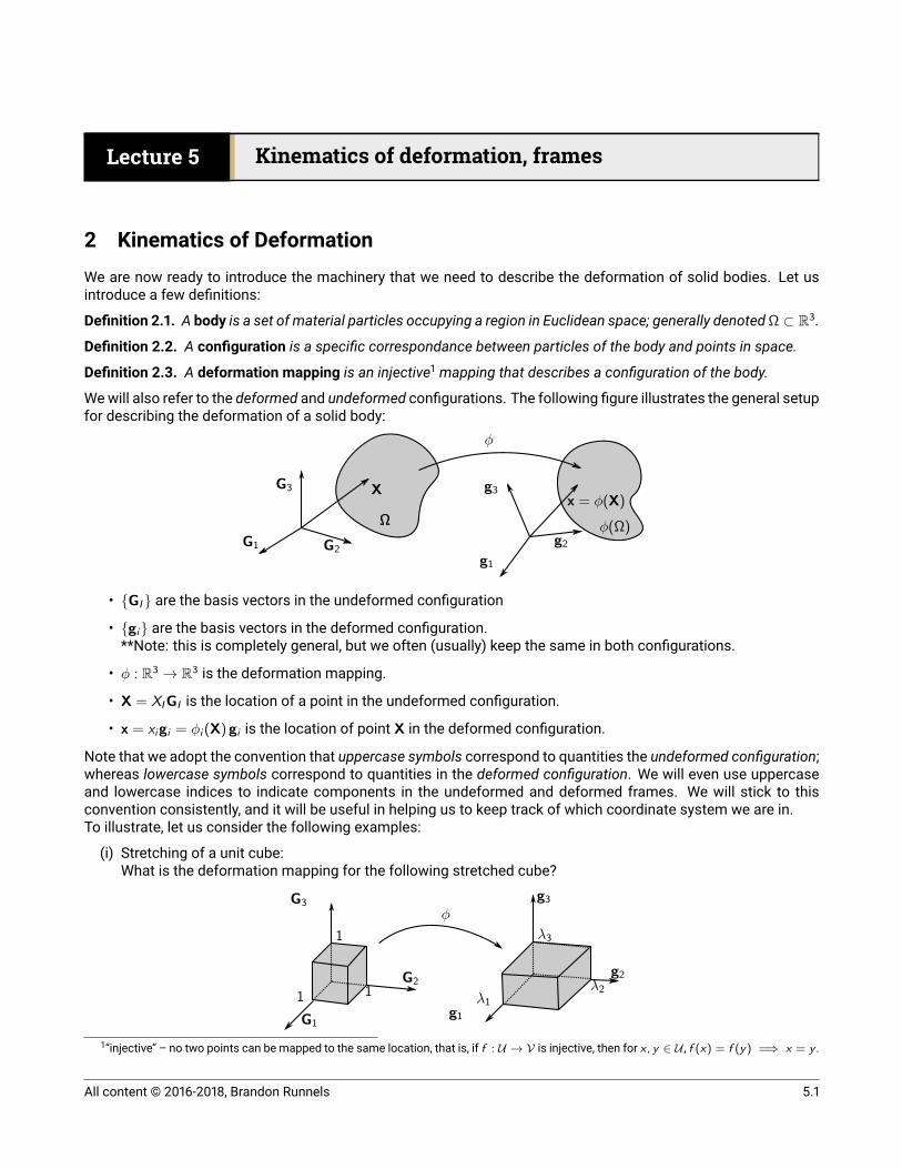
2 Kinematics of DeformationWe are now ready to introduce the machinery that we need to describe the deformation of solid bodies. Let usintroduce a few definitions:Definition 2.1. A body is a set of material particles occupying a region in Euclidean space; generally denoted Ω ⊂ R3.Definition 2.2. A configuration is a specific correspondance between particles of the body and points in space.Definition 2.3. A deformation mapping is an injective1 mapping that describes a configuration of the body.Wewill also refer to the deformed and undeformed configurations. The following figure illustrates the general setupfor describing the deformation of a solid body:
G1 G2
G3
g1
g2
g3
φ
ΩΩ φ(Ω)
Xx = φ(X)
• GI are the basis vectors in the undeformed configuration• gi are the basis vectors in the deformed configuration.**Note: this is completely general, but we often (usually) keep the same in both configurations.• φ : R3 → R3 is the deformation mapping.• X = XIGI is the location of a point in the undeformed configuration.• x = xigi = φi (X) gi is the location of point X in the deformed configuration.
Note that we adopt the convention that uppercase symbols correspond to quantities the undeformed configuration;whereas lowercase symbols correspond to quantities in the deformed configuration. We will even use uppercaseand lowercase indices to indicate components in the undeformed and deformed frames. We will stick to thisconvention consistently, and it will be useful in helping us to keep track of which coordinate system we are in.To illustrate, let us consider the following examples:(i) Stretching of a unit cube:What is the deformation mapping for the following stretched cube?
G1
G2
G3
g1
g2
g3
1 1
1
λ1
λ2
λ3
φ
1“injective” – no two points can be mapped to the same location, that is, if f : U → V is injective, then for x , y ∈ U , f (x) = f (y) =⇒ x = y .
All content © 2016-2018, Brandon Runnels 5.1
MAE 5100 - Continuum MechanicsUniversity of Colorado Colorado Springs Course Notes - Lecture 5solids.uccs.edu/teaching/mae5100
(Notice that g1 = G1, etc.) We identify the deformation mapping simply asx1 = λ1 X1 x2 = λ1 X2 x3 = λ1 X3 (2.1)
Or, we can describe this asx = φ(X) =
[λ1 0 00 λ2 00 0 λ3
]X = F X (2.2)
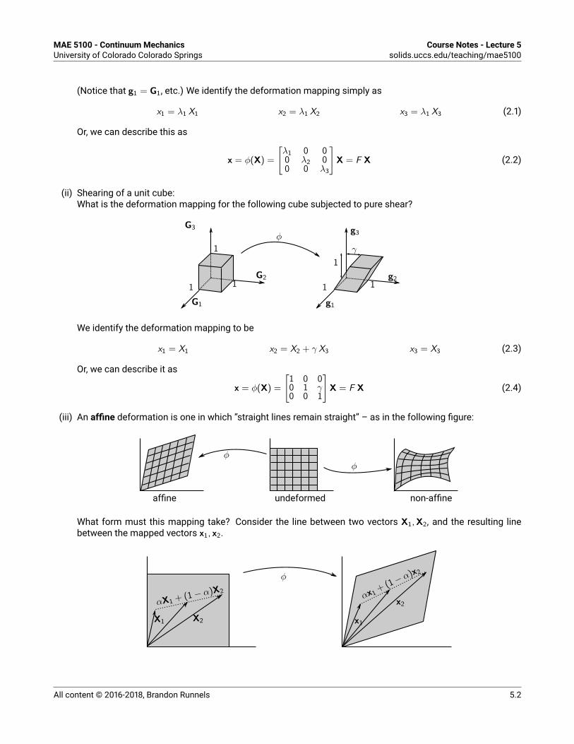
(ii) Shearing of a unit cube:What is the deformation mapping for the following cube subjected to pure shear?
G1
G2
G3
1 1
1
φ
g1
g2
g3
1 1
γ
1
We identify the deformation mapping to bex1 = X1 x2 = X2 + γ X3 x3 = X3 (2.3)
Or, we can describe it asx = φ(X) =
[1 0 00 1 γ0 0 1
]X = F X (2.4)
(iii) An affine deformation is one in which “straight lines remain straight” – as in the following figure:
undeformedaffine non-affine
φφ
What form must this mapping take? Consider the line between two vectors X1,X2, and the resulting linebetween the mapped vectors x1, x2.
φ
X1
x2
X2
αX1 + (1− α)X2
x1
αx1+ (1−
α)x2
All content © 2016-2018, Brandon Runnels 5.2
MAE 5100 - Continuum MechanicsUniversity of Colorado Colorado Springs Course Notes - Lecture 5solids.uccs.edu/teaching/mae5100
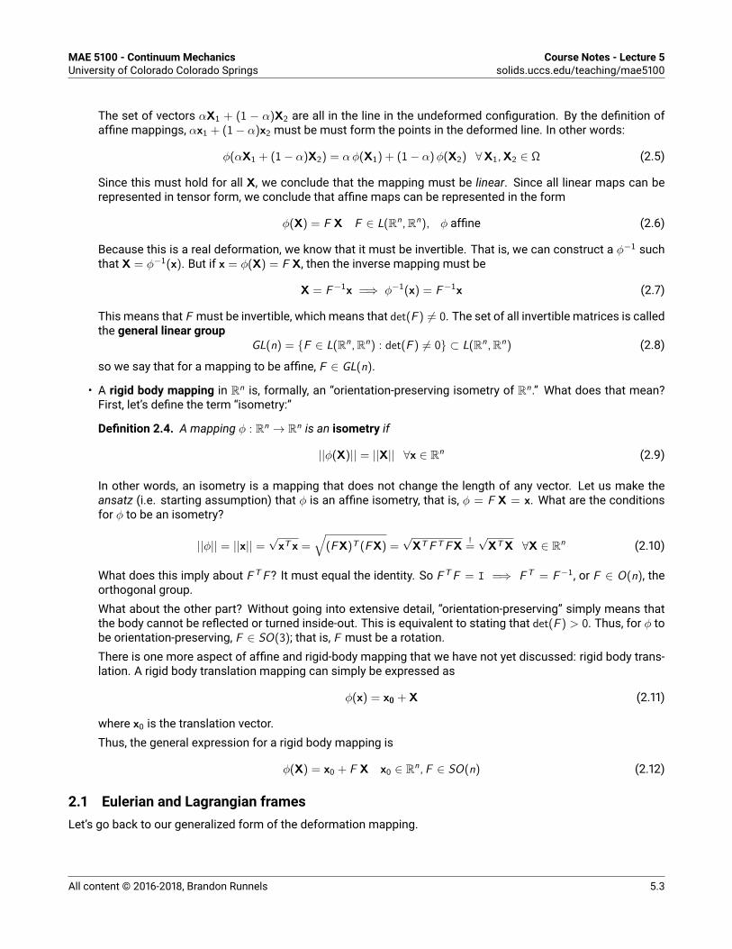
The set of vectors αX1 + (1 − α)X2 are all in the line in the undeformed configuration. By the definition ofaffine mappings, αx1 + (1− α)x2 must be must form the points in the deformed line. In other words:φ(αX1 + (1− α)X2) = αφ(X1) + (1− α)φ(X2) ∀X1,X2 ∈ Ω (2.5)
Since this must hold for all X, we conclude that the mapping must be linear. Since all linear maps can berepresented in tensor form, we conclude that affine maps can be represented in the formφ(X) = F X F ∈ L(Rn,Rn), φ affine (2.6)
Because this is a real deformation, we know that it must be invertible. That is, we can construct a φ−1 suchthat X = φ−1(x). But if x = φ(X) = F X, then the inverse mapping must beX = F−1x =⇒ φ−1(x) = F−1x (2.7)
This means that F must be invertible, which means that det(F ) 6= 0. The set of all invertible matrices is calledthe general linear groupGL(n) = F ∈ L(Rn,Rn) : det(F ) 6= 0 ⊂ L(Rn,Rn) (2.8)
so we say that for a mapping to be affine, F ∈ GL(n).• A rigid body mapping in Rn is, formally, an “orientation-preserving isometry of Rn.” What does that mean?First, let’s define the term “isometry:”Definition 2.4. A mapping φ : Rn → Rn is an isometry if
||φ(X)|| = ||X|| ∀x ∈ Rn (2.9)In other words, an isometry is a mapping that does not change the length of any vector. Let us make theansatz (i.e. starting assumption) that φ is an affine isometry, that is, φ = F X = x. What are the conditionsfor φ to be an isometry?
||φ|| = ||x|| =√xTx =
√(FX)T (FX) =
√XTFTFX
!=√XTX ∀X ∈ Rn (2.10)
What does this imply about FTF? It must equal the identity. So FTF = I =⇒ FT = F−1, or F ∈ O(n), theorthogonal group.What about the other part? Without going into extensive detail, “orientation-preserving” simply means thatthe body cannot be reflected or turned inside-out. This is equivalent to stating that det(F ) > 0. Thus, for φ tobe orientation-preserving, F ∈ SO(3); that is, F must be a rotation.There is one more aspect of affine and rigid-body mapping that we have not yet discussed: rigid body trans-lation. A rigid body translation mapping can simply be expressed as
φ(x) = x0 + X (2.11)where x0 is the translation vector.Thus, the general expression for a rigid body mapping is
φ(X) = x0 + F X x0 ∈ Rn,F ∈ SO(n) (2.12)2.1 Eulerian and Lagrangian framesLet’s go back to our generalized form of the deformation mapping.
All content © 2016-2018, Brandon Runnels 5.3
MAE 5100 - Continuum MechanicsUniversity of Colorado Colorado Springs Course Notes - Lecture 5solids.uccs.edu/teaching/mae5100
G1 G2
G3
g1
g2
g3
φ
ΩΩ φ(Ω)
Xx = φ(X)
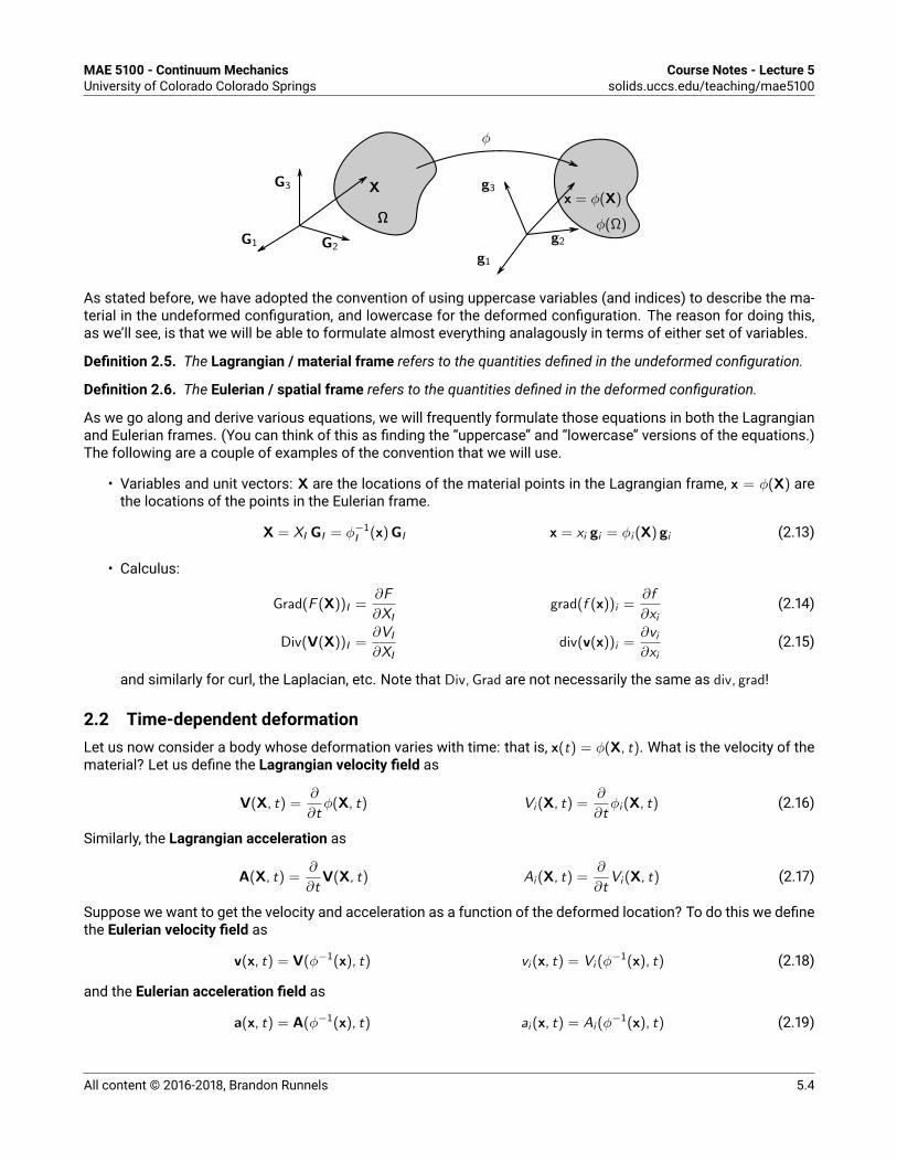
As stated before, we have adopted the convention of using uppercase variables (and indices) to describe the ma-terial in the undeformed configuration, and lowercase for the deformed configuration. The reason for doing this,as we’ll see, is that we will be able to formulate almost everything analagously in terms of either set of variables.Definition 2.5. The Lagrangian / material frame refers to the quantities defined in the undeformed configuration.
Definition 2.6. The Eulerian / spatial frame refers to the quantities defined in the deformed configuration.
As we go along and derive various equations, we will frequently formulate those equations in both the Lagrangianand Eulerian frames. (You can think of this as finding the “uppercase” and “lowercase” versions of the equations.)The following are a couple of examples of the convention that we will use.• Variables and unit vectors: X are the locations of the material points in the Lagrangian frame, x = φ(X) arethe locations of the points in the Eulerian frame.
X = XI GI = φ−1I (x)GI x = xi gi = φi (X) gi (2.13)
• Calculus:Grad(F (X))I =
∂F
∂XIgrad(f (x))i =
∂f
∂xi(2.14)
Div(V(X))I =∂VI
∂XIdiv(v(x))i =
∂vi∂xi
(2.15)and similarly for curl, the Laplacian, etc. Note that Div, Grad are not necessarily the same as div, grad!
2.2 Time-dependent deformationLet us now consider a body whose deformation varies with time: that is, x(t) = φ(X, t). What is the velocity of thematerial? Let us define the Lagrangian velocity field as
V(X, t) =∂
∂tφ(X, t) Vi (X, t) =
∂
∂tφi (X, t) (2.16)
Similarly, the Lagrangian acceleration asA(X, t) =
∂
∂tV(X, t) Ai (X, t) =
∂
∂tVi (X, t) (2.17)
Suppose we want to get the velocity and acceleration as a function of the deformed location? To do this we definethe Eulerian velocity field asv(x, t) = V(φ−1(x), t) vi (x, t) = Vi (φ
−1(x), t) (2.18)and the Eulerian acceleration field as
a(x, t) = A(φ−1(x), t) ai (x, t) = Ai (φ−1(x), t) (2.19)
All content © 2016-2018, Brandon Runnels 5.4
Lecture 6 Material derivative, metric changes
Example 2.1
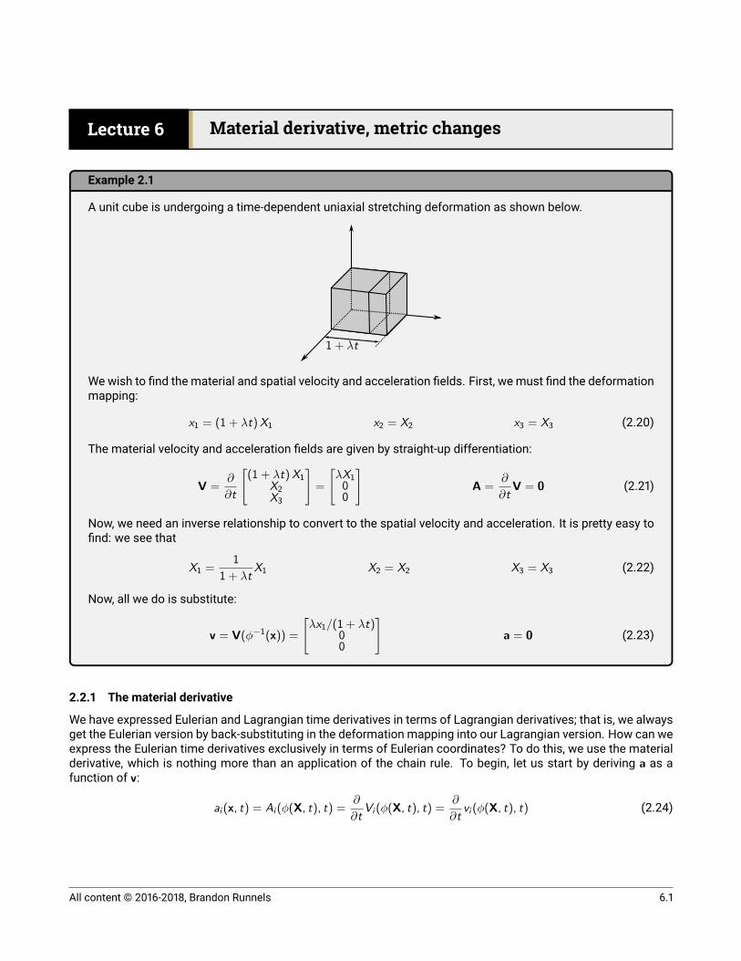
A unit cube is undergoing a time-dependent uniaxial stretching deformation as shown below.
1 + λt
Wewish to find the material and spatial velocity and acceleration fields. First, we must find the deformationmapping:x1 = (1 + λt)X1 x2 = X2 x3 = X3 (2.20)
The material velocity and acceleration fields are given by straight-up differentiation:V =
∂
∂t
[(1 + λt)X1
X2X3
]=
[λX1
00
]A =
∂
∂tV = 0 (2.21)
Now, we need an inverse relationship to convert to the spatial velocity and acceleration. It is pretty easy tofind: we see thatX1 =
1
1 + λtX1 X2 = X2 X3 = X3 (2.22)
Now, all we do is substitute:v = V(φ−1(x)) =
[λx1/(1 + λt)
00
]a = 0 (2.23)
2.2.1 The material derivative
We have expressed Eulerian and Lagrangian time derivatives in terms of Lagrangian derivatives; that is, we alwaysget the Eulerian version by back-substituting in the deformation mapping into our Lagrangian version. How can weexpress the Eulerian time derivatives exclusively in terms of Eulerian coordinates? To do this, we use the materialderivative, which is nothing more than an application of the chain rule. To begin, let us start by deriving a as afunction of v:ai (x, t) = Ai (φ(X, t), t) =
∂
∂tVi (φ(X, t), t) =
∂
∂tvi (φ(X, t), t) (2.24)
All content © 2016-2018, Brandon Runnels 6.1
MAE 5100 - Continuum MechanicsUniversity of Colorado Colorado Springs Course Notes - Lecture 6solids.uccs.edu/teaching/mae5100
Apply the chain rule:=∂vi∂xj
∂xj∂t︸︷︷︸=vj
+∂vi∂t
=∂vi∂xj
vi +∂vi∂t
= vi ,jvj + vi ,t (2.25)
Or, in invariant notation,a = grad(v) v +
∂
∂tv (2.26)
The material derivative is just the generalization of this chain rule. Let f (x, t) be some function (scalar or vector).Then we define the material (time) derivative asDf
Dt=∂f
∂xjvj +
∂f
∂t(2.27)
It may be useful to note that there is nothing really special about the material time derivative. As we saw earlier,the Lagrangian/Eulerian acceleration/velocity fields are nicely derived in the material frame as straight-up timederivatives. The material time derivative is just what happens when we decide we want to work in the Eulerianframe only: suddenly, everything becomes more complicated becuase the spatial coordinates themselves dependon time.Example 2.2
Continuing with our previous example, let us prove that we recover a using the material time derivative.
a1 =∂v1
∂x1v1 +7
0∂v1
∂x2v2 +7
0∂v1
∂x3v3 +
∂v1
∂t=( λ
1 + λt
)( λx1
1 + λt
)+(− λx1
(1 + λt)2(λ)) (2.28)
=λ2x1
(1 + λt)2− λ2x1
(1 + λt)2= 0 X (2.29)
The other components are all zero, so their derivatives will be zero as well.
2.3 Kinematics of local deformationLet us consider the case of all deformations, affine and otherwise. Affine deformations are fairly easy to quantify:thematerial deforms the sameway at everymaterial point, andwe can easily represent themapping using a tensor.The general case is more complicated, but it is what we are interested in.Before discussing local deformation, let us briefly discuss Taylor series. You may recall from Caclulus that anysufficiently smooth function, f (x), can be represented as a Taylor expansion about a point a as follows:
f (x) = f (a) + f ′(x)(x − a) +1
2f ′′(x)(x − a)2 + ... =
∞∑n=1
1
n!
∂n
∂xn(x − a)n (2.30)
We can do a similar thing withmultivariate functions: let f : Rn → R. Then the expansion of f about a pointX0 ∈ Rn
isf (X) = f (X0) +
∂f
∂XI(XI − X 0
I ) +1
2
∂2f
∂XI∂XJ(XI − X 0
I )(XJ − X 0J ) + higher order terms (2.31)
All content © 2016-2018, Brandon Runnels 6.2
MAE 5100 - Continuum MechanicsUniversity of Colorado Colorado Springs Course Notes - Lecture 6solids.uccs.edu/teaching/mae5100
or, using invariant notation,= f (X0) + Grad(f )(X− X0) +
1
2(X− X0)T Grad(Grad(f ))(X− X0) + higher order terms (2.32)
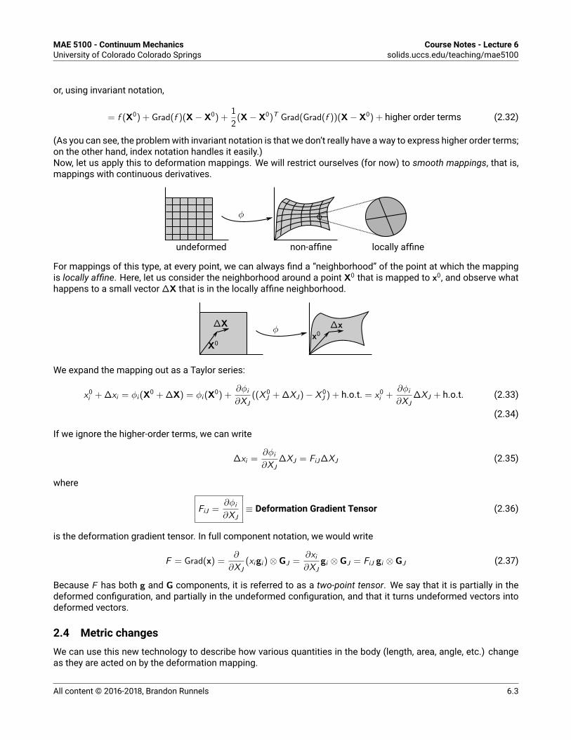
(As you can see, the problemwith invariant notation is that we don’t really have a way to express higher order terms;on the other hand, index notation handles it easily.)Now, let us apply this to deformation mappings. We will restrict ourselves (for now) to smooth mappings, that is,mappings with continuous derivatives.
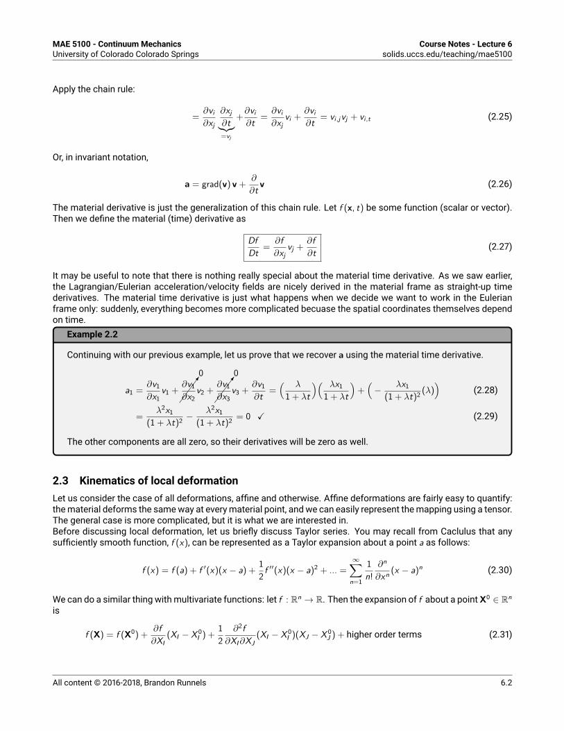
undeformed non-affine
φ
locally affineFor mappings of this type, at every point, we can always find a “neighborhood” of the point at which the mappingis locally affine. Here, let us consider the neighborhood around a point X0 that is mapped to x0, and observe whathappens to a small vector ∆X that is in the locally affine neighborhood.
φ
X0
∆X ∆xx0
We expand the mapping out as a Taylor series:x0i + ∆xi = φi (X
0 + ∆X) = φi (X0) +
∂φi∂XJ
((X 0J + ∆XJ)− X 0
J ) + h.o.t. = x0i +
∂φi∂XJ
∆XJ + h.o.t. (2.33)(2.34)
If we ignore the higher-order terms, we can write∆xi =
∂φi∂XJ
∆XJ = FiJ∆XJ (2.35)where
FiJ =∂φi∂XJ
≡ Deformation Gradient Tensor (2.36)is the deformation gradient tensor. In full component notation, we would write
F = Grad(x) =∂
∂XJ(xigi )⊗ GJ =
∂xi∂XJ
gi ⊗ GJ = FiJ gi ⊗ GJ (2.37)Because F has both g and G components, it is referred to as a two-point tensor. We say that it is partially in thedeformed configuration, and partially in the undeformed configuration, and that it turns undeformed vectors intodeformed vectors.2.4 Metric changesWe can use this new technology to describe how various quantities in the body (length, area, angle, etc.) changeas they are acted on by the deformation mapping.All content © 2016-2018, Brandon Runnels 6.3
MAE 5100 - Continuum MechanicsUniversity of Colorado Colorado Springs Course Notes - Lecture 6solids.uccs.edu/teaching/mae5100
2.4.1 Change of length
Let us begin by considering a small vector ∆X in the neighborhood of X as we had before. What is the change inlength as ∆X is acted on by φ? Let F = F (X) be the local deformation gradient. Then||∆x|| =
√∆xk∆xk =
√(FkI∆XI )(FkJ∆XJ) =
√∆XIFT
Ik FkJ∆XJ =√
∆XTFTF∆X =√
∆XTC∆X (2.38)where
C = FTF CIJ = FTIk FkJ ≡ Right Cauchy-Green Deformation Tensor (2.39)
Notice that C has strictly uppercase indices: this implies that it lives entirely in the Lagrangian frame. If we divideboth sides by ∆x, we have||∆x||2
||∆X||2= NICIJNJ = NTC N = λ2(N) ≡ Stretch Ratio (2.40)
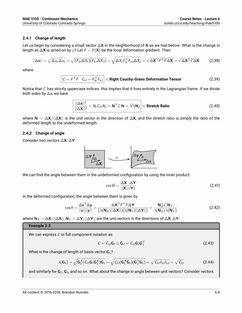
where N = ∆X/||∆X|| is the unit vector in the direction of ∆X, and the stretch ratio is simply the ratio of thedeformed length to the undeformed length.2.4.2 Change of angle
Consider two vectors ∆X, ∆Y.
φ
∆X∆x
∆Y ∆yΘ θ
We can find the angle between them in the undeformed configuration by using the inner product:cos Θ =
∆X ·∆Y
||X||||Y||(2.41)
In the deformed configuration, the angle between them is given bycos θ =
∆xT∆y
||x||||y||=
∆XTFTF∆Y
(λ(NX )||∆X||)(λ(NY )||∆Y||)=
NTXC NY
λ(NX )λ(NY )(2.42)
where NX = ∆X/||∆X||,NY = ∆Y/||∆Y|| are the unit vectors in the directions of ∆X, ∆Y.Example 2.3
We can express C in full component notation asC = CIJGI ⊗ GJ = CIJGIG
TJ (2.43)
What is the change of length of basis vector G1?λ(G1) =
√GT
1 (CIJGIGTJ )G1 =
√CIJ(GT
1 GI )(GTJ G1) =
√CIJδ1I δ1J =
√C11 (2.44)
and similarly for G2,G3, and so on. What about the change in angle between unit vectors? Consider vectors
All content © 2016-2018, Brandon Runnels 6.4
MAE 5100 - Continuum MechanicsUniversity of Colorado Colorado Springs Course Notes - Lecture 6solids.uccs.edu/teaching/mae5100
GP ,GQ . The change in angle iscos θPQ =
GTPC GQ
λ(GP)λ(GQ)no sum on P, Q (2.45)
=CPQ
CPPCQQno sum on P, Q (2.46)
We notice a general trend here, as with the deformation gradient: diagonal terms relate to elongation,whereas off-diagonal terms relate to shear.
All content © 2016-2018, Brandon Runnels 6.5
Lecture 7 Metric changes, eigenvalues, eigenvectors
2.4.3 Determinant identities
Recall the formulae for the determinant of a tensor F ∈ L(R3,R3):det(F ) = εijkFi1Fj2Fk3 det(F ) =
1
6εijkεIJKFiIFjJFkK (2.47)
Identity:εijkFiIFjJFkK =
+ det(F ) IJK = 123, 231, 312
− det(F ) IJK = 321, 132, 213
0 else= det(F ) εIJK (2.48)
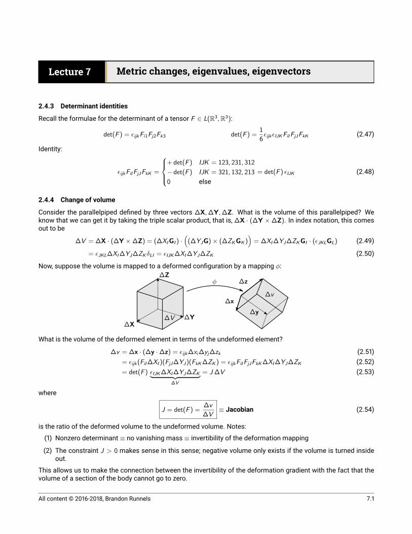
2.4.4 Change of volume
Consider the parallelpiped defined by three vectors ∆X, ∆Y, ∆Z. What is the volume of this parallelpiped? Weknow that we can get it by taking the triple scalar product, that is, ∆X · (∆Y ×∆Z). In index notation, this comesout to be∆V = ∆X · (∆Y ×∆Z) = (∆XIGI ) ·
((∆YJG)× (∆ZKGK )
)= ∆XI∆YJ∆ZKGI · (εJKLGL) (2.49)
= εJKL∆XI∆YJ∆ZKδLI = εIJK∆XI∆YJ∆ZK (2.50)Now, suppose the volume is mapped to a deformed configuration by a mapping φ:
∆X
∆Z
∆Y∆y
∆x
∆z
∆V
∆v
φ
What is the volume of the deformed element in terms of the undeformed element?∆v = ∆x · (∆y ·∆z) = εijk∆xi∆yj∆zk (2.51)
= εijk(FiI∆XI )(FjJ∆YJ)(FkK∆ZK ) = εijkFiIFjJFkK∆XI∆YJ∆ZK (2.52)= det(F ) εIJK∆XI∆YJ∆ZK︸ ︷︷ ︸
∆V
= J ∆V (2.53)where
J = det(F ) =∆v
∆V≡ Jacobian (2.54)
is the ratio of the deformed volume to the undeformed volume. Notes:(1) Nonzero determinant ≡ no vanishing mass ≡ invertibility of the deformation mapping(2) The constraint J > 0 makes sense in this sense; negative volume only exists if the volume is turned insideout.
This allows us to make the connection between the invertibility of the deformation gradient with the fact that thevolume of a section of the body cannot go to zero.All content © 2016-2018, Brandon Runnels 7.1
MAE 5100 - Continuum MechanicsUniversity of Colorado Colorado Springs Course Notes - Lecture 7solids.uccs.edu/teaching/mae5100
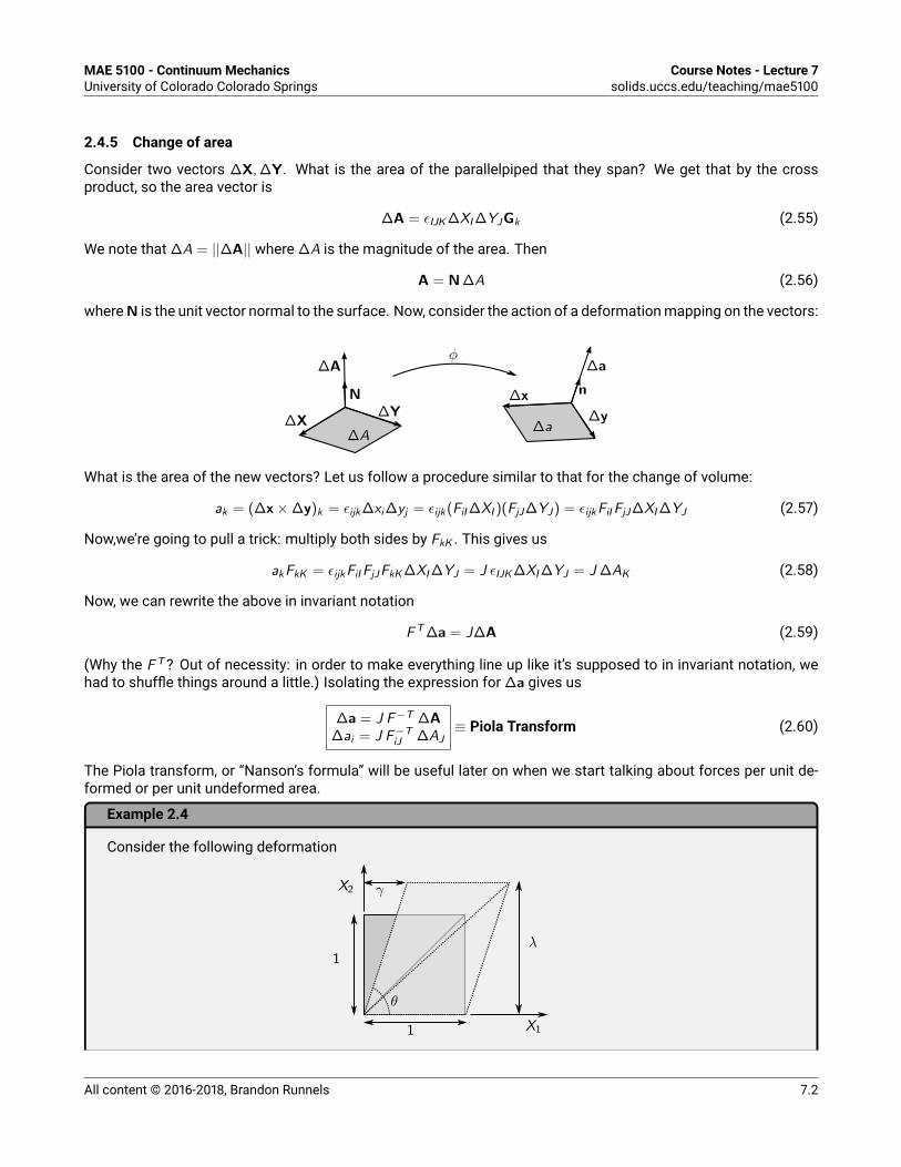
2.4.5 Change of area
Consider two vectors ∆X, ∆Y. What is the area of the parallelpiped that they span? We get that by the crossproduct, so the area vector is∆A = εIJK∆XI∆YJGk (2.55)
We note that ∆A = ||∆A|| where ∆A is the magnitude of the area. ThenA = N∆A (2.56)
whereN is the unit vector normal to the surface. Now, consider the action of a deformationmapping on the vectors:
∆X∆Y
∆Aφ
∆A
∆x
∆y
∆a
∆a
N n
What is the area of the new vectors? Let us follow a procedure similar to that for the change of volume:ak = (∆x×∆y)k = εijk∆xi∆yj = εijk(FiI∆XI )(FjJ∆YJ) = εijkFiIFjJ∆XI∆YJ (2.57)
Now,we’re going to pull a trick: multiply both sides by FkK . This gives usakFkK = εijkFiIFjJFkK∆XI∆YJ = J εIJK∆XI∆YJ = J ∆AK (2.58)
Now, we can rewrite the above in invariant notationFT∆a = J∆A (2.59)
(Why the FT ? Out of necessity: in order to make everything line up like it’s supposed to in invariant notation, wehad to shuffle things around a little.) Isolating the expression for ∆a gives us∆a = J F−T ∆A
∆ai = J F−TiJ ∆AJ≡ Piola Transform (2.60)
The Piola transform, or “Nanson’s formula” will be useful later on when we start talking about forces per unit de-formed or per unit undeformed area.Example 2.4
Consider the following deformation
λ
γ
1
1
X1
X2
θ
All content © 2016-2018, Brandon Runnels 7.2
MAE 5100 - Continuum MechanicsUniversity of Colorado Colorado Springs Course Notes - Lecture 7solids.uccs.edu/teaching/mae5100
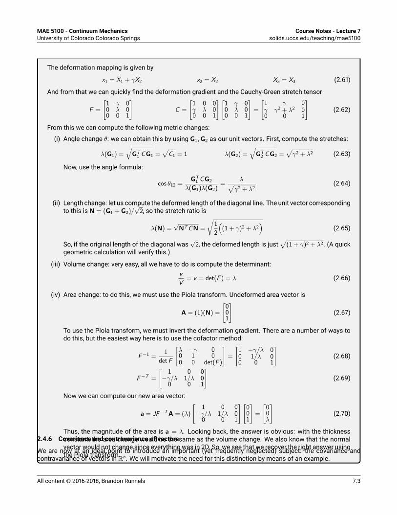
The deformation mapping is given byx1 = X1 + γX2 x2 = X2 X3 = X3 (2.61)
And from that we can quickly find the deformation gradient and the Cauchy-Green stretch tensorF =
[1 γ 00 λ 00 0 1
]C =
[1 0 0γ λ 00 0 1
][1 γ 00 λ 00 0 1
]=
[1 γ 0γ γ2 + λ2 00 0 1
](2.62)
From this we can compute the following metric changes:(i) Angle change θ: we can obtain this by using G1,G2 as our unit vectors. First, compute the stretches:
λ(G1) =√GT
1 CG1 =√C1 = 1 λ(G2) =
√GT
2 CG2 =√γ2 + λ2 (2.63)
Now, use the angle formula:cos θ12 =
GT1 CG2
λ(G1)λ(G2)=
λ√γ2 + λ2
(2.64)(ii) Length change: let us compute the deformed length of the diagonal line. The unit vector correspondingto this is N = (G1 + G2)/
√2, so the stretch ratio is
λ(N) =√NTCN =
√1
2
((1 + γ)2 + λ2
) (2.65)So, if the original length of the diagonal was√2, the deformed length is just√(1 + γ)2 + λ2. (A quickgeometric calculation will verify this.)
(iii) Volume change: very easy, all we have to do is compute the determinant:v
V= v = det(F ) = λ (2.66)
(iv) Area change: to do this, we must use the Piola transform. Undeformed area vector isA = (1)(N) =
[001
](2.67)
To use the Piola transform, we must invert the deformation gradient. There are a number of ways todo this, but the easiest way here is to use the cofactor method:F−1 =
1
detF
[λ −γ 00 1 00 0 det(F )
]=
[1 −γ/λ 00 1/λ 00 0 1
](2.68)
F−T =
[1 0 0−γ/λ 1/λ 0
0 0 1
](2.69)
Now we can compute our new area vector:a = JF−TA = (λ)
[1 0 0−γ/λ 1/λ 0
0 0 1
][001
]=
[00λ
](2.70)
Thus, the magnitude of the area is a = λ. Looking back, the answer is obvious: with the thicknessconstant, the area change would be the same as the volume change. We also know that the normalvector would not change since everything was in 2D. So, we see that we recover the right answer usingthe Piola transform.2.4.6 Covariance and contravariance of vectors
We are now at an ideal point to introduce an important (yet frequently neglected) subject: the covariance andcontravariance of vectors in Rn. We will motivate the need for this distinction by means of an example.
All content © 2016-2018, Brandon Runnels 7.3
MAE 5100 - Continuum MechanicsUniversity of Colorado Colorado Springs Course Notes - Lecture 7solids.uccs.edu/teaching/mae5100
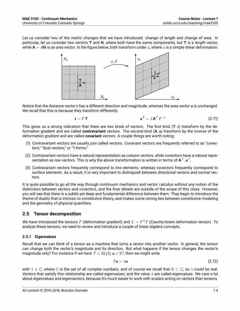
Let us consider two of the metric changes that we have introduced: change of length and change of area. Inparticular, let us consider two vectors T and N, where both have the same components, but T is a length vector,whileA = AN is an area vector. In the figure below, both transform under φ, where φ is a simple shear deformation:
X1
X2 x2
x1
AT
t
a
φ,F
Notice that the distance vector t has a different direction and magnitude, whereas the area vector a is unchanged.We recall that this is because they transform differently:t = F T aT = J AT F−1 (2.71)
This gives us a strong indication that there are two kinds of vectors. The first kind (T, t) transform by the de-formation gradient and are called contravariant vectors. The second kind (A, a) transform by the inverse of thedeformation gradient and are called covariant vectors. A couple things are worth noting:(1) Contravariant vectors are usually just called vectors. Covariant vectors are frequently referred to as “covec-tors,” “dual vectors,” or “1-forms.”(2) Contravariant vectors have a natural representation as column vectors, while covectors have a natural repre-sentation as row vectors. This is why the above transformation is written in terms of AT , aT .(3) Contravariant vectors frequently correspond to line elements, whereas covectors frequently correspond to
surface elements. As a result, it is very important to distinguish between directional vectors and normal vec-tors.It is quite possible to go all the way through continuum mechanics and vector calculus without any notion of thedistinction between vectors and covectors, and the finer details are outside of the scope of this class. However,you will see that there is a subtle yet deep and fundamental difference between them. They begin to introduce thetheme of duality that is intrinsic to constitutive theory, and makes some strong ties between constitutive modelingand the geometry of physical quantities.2.5 Tensor decompositionWe have introduced the tensors F (deformation gradient) and C = FTF (Cauchy-Green deformation tensor). Toanalyze these tensors, we need to review and introduce a couple of linear algebra concepts.2.5.1 Eigenvalues
Recall that we can think of a tensor as a machine that turns a vector into another vector. In general, the tensorcan change both the vector’s magnitude and its direction. But what happens if the tensor changes the vector’smagnitude only? For instance if we have T ∈ GL(3),u ∈ R3, then we might writeTu = λu (2.72)
with λ ∈ C, where C is the set of all complex numbers, and of course we recall that R ⊂ C, so λ could be real.Vectors that satisfy this relationship are called eigenvalues, and the value λ are called eigenvalues. We care a lotabout eigenvalues and eigenvectors, because it’s much easier to work with scalars acting on vectors than tensors.All content © 2016-2018, Brandon Runnels 7.4
MAE 5100 - Continuum MechanicsUniversity of Colorado Colorado Springs Course Notes - Lecture 7solids.uccs.edu/teaching/mae5100
How do we go about finding these eigenvalues and eigenvectors? We know that they will satisfy the equationTu− λu = (T − λI)u = 0 (2.73)
Of course, one solution is that u is just zero, but this isn’t very interesting at all because the result would be trivial.Instead, we notice that the matrix T − λI is able to take a non-zero vector and spit out zero. We say that u is in the“nullspace” or “kernel” of T − λI, and there’s a nice theorem (called the “Rank-Nullity theorem” that unfortunatelywe don’t have time to prove here) that tells us that the tensor T − λI can map a vector u to zero if and only ifdet(T − λI) = 0. This means that we can now solve the algebraic equation
det(T − λI) = 0 (2.74)which is a nth order polynomial. We know that we will find at least one, and no more than three eigenvalues λi bysolving this equation. We can then find our eigenvectors ui by solving
Tui = λ(i)u(i) (2.75)An interesting side note is the following: we can always write
det(T − λI) = c3λ3 + c2λ
2 + c1λ+ c0 = 0 (2.76)where (2.76) is the characteristic equation and
• c3 = 1
• c2 = I1 = tr(T ) ≡ the first invariant of T• c1 = I2 = 1
2 (tr(T )2 − tr(TT )) ≡ the second invariant of T• c0 = −I3 = − det(T ) ≡ the (negative) third invariant of T
All content © 2016-2018, Brandon Runnels 7.5
Lecture 8 Tensor properties and the spectral theorem
We will continue with our introduction to tensor decomposition. The following theorem is an interesting side noteto the discussion of a tensor’s characteristic equation:Theorem 2.1 (Cayley-Hamilton). Every square tensor T ∈ L(Rn,Rn) satisfies its own characteristic equation.
We will also introduce another theorem without proof:Theorem 2.2. Every square tensor T ∈ L(Rn,Rn) has n linearly independent eigenvectors.
This will come in handy in following sections.2.5.2 Symmetric and positive definite tensors
We recall the definition for a symmetric matrix:Definition 2.7. A square tensor T is symmetric if T = TT . If T is symmetric and has components Tij in anorthonormal basis, then Tij = Tji
We note the following important identity: if T is symmetric, then for u, v ∈ Rn we can always writeuTTv = uTTTv = (Tu)Tv (2.77)
Let us make another very important definition:Definition 2.8. A square tensor T ∈ L(Rn,Rn) is positive definite if
uTTu > 0 ∀u ∈ Rn, ||u|| > 0 (2.78)and
uTAu = 0 =⇒ ||u|| = 0 (2.79)(An important equivalence to note here is that a matrix is positive definite if and only if all of its eigenvalues arereal and strictly positive.) Finally, we will make one more similar definition:Definition 2.9. A square tensor T ∈ L(Rn,Rn) is positive semidefinite if
uTAu ≥ 0 ∀u ∈ Rn (2.80)Note that the only difference is that this allows for nonzero vectors to be mapped to zero. Matrices are positivesemidefinite if and only iff all of its eigenvalues are real and nonnegative, i.e. it can have eigenvalues with valuezero.2.5.3 Spectral theorem (symmetric tensors)
The spectral theorem is one of themost powerful theorems in appliedmathematics. It haswidespread applicationsbeyond matrices, such as the Fourier and Laplace transforms, or Sturm-Liouville theory. If you haven’t taken a(graduate level) linear algebra course, you should definitely consider taking one.The first theorem we will introduce without proof:Theorem 2.3 (Real eigenvalues). If a tensor T is symmetric, all of its eigenvalues are real.
The proof of this theorem is quite easy, but it involves the use of complex analysis which is a bit beyond the scopeof the course right now. The next theorem is very important, and so we will prove it.
All content © 2016-2018, Brandon Runnels 8.1
MAE 5100 - Continuum MechanicsUniversity of Colorado Colorado Springs Course Notes - Lecture 8solids.uccs.edu/teaching/mae5100
Theorem 2.4 (Orthogonal eigenvectors). If a nxn tensor T is symmetric, it has n orthonormal eigenvectors.Proof. We will look at two cases.(1) Distinct eigenvalues: let ui be the eigenvectors of T corresponding to the distinct eigenvalues λi, that is,no two eigenvalues are the same. Now, let us consider two eigenvectors ui ,uj with eigenvalues λi ,λj ,λi 6= λj .Because the matrix is symmetric, we can write
0 = uTi Auj − (Aui )TAuj = ui (λ(j)uj)− (λ(i)u(i))
Tuj = (λ(i) − λ(j))(uT(i)u(j)) = 0 (2.81)Since λi 6= λj , the only way for this to be true is for ui to be orthogonal to uj .
(2) Degenerate eigenvalues: let ui ,uj be two eigenvectors ofT bothwith eigenvalue λ. Thenwe canwrite, ∀α,β ∈R,
T (αui + βuj) = αTui + βTuj = λ(αui + βuj) (2.82)In other words, every vector αui + βuj is an eigenvector of T . More generally, we can write that
Tu = λu ∀u ∈ span(ui ,uj) (2.83)that is, that there is a 2D space of eigenvectors of T with eigenvalue λ. We know from linear algebra thatthere exists an orthonormal basis for this space; this orthonormal basis gives the orthogonal eigenvectorsfor T . The case of 3+ degenerate eigenvalues proceeds by induction.
Now that we know that every symmetric matrix T has a set of orthonormal eigenvectors, we can use these eigen-vectors to construct an orthonormal basis. We call this the eigenbasis of T .Theorem2.5 (Spectral decomposition). AsymmetricmatrixT can be expressed strictly in termsof rotationmatricesconstructed from its eigenvectors and a diagonal matrix with each diagonal entry containing an eigenvalue of T .Proof. Let us consider the action of T on any vector x ∈ Rn. By casting x into the eigenbasis of T , then by findingthe action of T on its eigenvectors, and finally casting back, we obtain
Tx = T (eixi ) = Tvj(vTj ei )xi =
∑j
λjvj(vTj ei )xi =
∑j
vjλj(vTj ei )xi =
∑j
ek(eTk vj)λj(vTj ei )xi (2.84)
Introducing a couple of Kronecker deltas and rearranging indices gives= ei (eTi vp)︸ ︷︷ ︸
QTip
(∑r
δprλrδrq
)︸ ︷︷ ︸
Λpq
(vTq ej)︸ ︷︷ ︸Qqj
xj (2.85)
concluding the proof.in other words, the components of T in the original basis can be expressed as
Tij = QTip ΛpqQqj (2.86)
where Q are orthogonal transformation matrices whose components are given in terms of the eigenvectors v byQ =
[v1 · e1 v1 · e2 v1 · e3v2 · e1 v2 · e2 v2 · e3v3 · e1 v3 · e2 v3 · e3
]=
vT1vT2vT3
(2.87)and Λ is a diagonal matrix with the eigenvalues λi along the diagonal. This is called diagonalization; it can also bereferred to as spectral decomposition or eigendecomposition.So what are we actually doing when we do an eigendecomposition? The important thing to remember is that weare not changing the tensor at all. Rather, we are finding a different way to express the tensor by decomposing itinto seperate stages. Consider the following illustration:All content © 2016-2018, Brandon Runnels 8.2
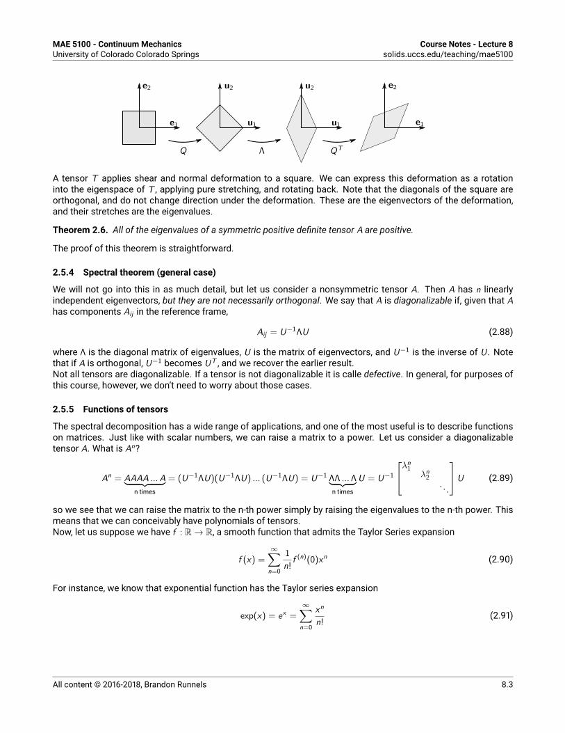
MAE 5100 - Continuum MechanicsUniversity of Colorado Colorado Springs Course Notes - Lecture 8solids.uccs.edu/teaching/mae5100
e1
e2
e1
e2
u1
u2
u1
u2
Q Λ QT
A tensor T applies shear and normal deformation to a square. We can express this deformation as a rotationinto the eigenspace of T , applying pure stretching, and rotating back. Note that the diagonals of the square areorthogonal, and do not change direction under the deformation. These are the eigenvectors of the deformation,and their stretches are the eigenvalues.Theorem 2.6. All of the eigenvalues of a symmetric positive definite tensor A are positive.
The proof of this theorem is straightforward.2.5.4 Spectral theorem (general case)
We will not go into this in as much detail, but let us consider a nonsymmetric tensor A. Then A has n linearlyindependent eigenvectors, but they are not necessarily orthogonal. We say that A is diagonalizable if, given that Ahas components Aij in the reference frame,Aij = U−1ΛU (2.88)
where Λ is the diagonal matrix of eigenvalues, U is the matrix of eigenvectors, and U−1 is the inverse of U . Notethat if A is orthogonal, U−1 becomes UT , and we recover the earlier result.Not all tensors are diagonalizable. If a tensor is not diagonalizable it is calle defective. In general, for purposes ofthis course, however, we don’t need to worry about those cases.2.5.5 Functions of tensors
The spectral decomposition has a wide range of applications, and one of the most useful is to describe functionson matrices. Just like with scalar numbers, we can raise a matrix to a power. Let us consider a diagonalizabletensor A. What is An?An = AAAA ...A︸ ︷︷ ︸
n times= (U−1ΛU)(U−1ΛU) ... (U−1ΛU) = U−1 ΛΛ ... Λ︸ ︷︷ ︸
n timesU = U−1
λn1 λn2 . . .U (2.89)
so we see that we can raise the matrix to the n-th power simply by raising the eigenvalues to the n-th power. Thismeans that we can conceivably have polynomials of tensors.Now, let us suppose we have f : R→ R, a smooth function that admits the Taylor Series expansionf (x) =
∞∑n=0
1
n!f (n)(0)xn (2.90)
For instance, we know that exponential function has the Taylor series expansionexp(x) = ex =
∞∑n=0
xn
n!(2.91)
All content © 2016-2018, Brandon Runnels 8.3
MAE 5100 - Continuum MechanicsUniversity of Colorado Colorado Springs Course Notes - Lecture 8solids.uccs.edu/teaching/mae5100
It turns out that we can use the Taylor series expansion to define functions ofmatrices. Supposewe have a functionf . Then we can describe the action of f on a diagonalizable tensor A by expanding in Taylor series form:
f (A) =∞∑n=0
1
n!f (n)(0)xn = U−1
∑∞
n=01n! f
(n)(0)λn1 ∑∞n=0
1n! f
(n)(0)λn2 . . .
U (2.92)
= U−1
f (λ1)f (λ2) . . .
U = U−1 f (Λ)U (2.93)
That is, we can describe the effect of a scalar function on a tensor, simply by taking the spectral decompositionand evaluating the function on each of the eigenvalues. For instance, if A ∈ L(R3,R3) is diagonalizable, we have√A = U−1
√λ1 √λ2 √
λ3
U, eA = U−1
eλ1
eλ2
eλ3
U, ln(A) = U−1
[ln(λ1)
ln(λ2)ln(λ3)
]U,
(2.94)and so on. Many of the same properties of f hold when extended to the matrix case, although it’s not always safeto make this generalization. For instance, if two tensors A,B have the same eigenbasis, you can even show thatsome properties of f such as eA+B = eAeB , ln(AB) = ln(A) + ln(B) hold; however, this is trickier if they do not.2.5.6 Polar decomposition
We work with a lot of very nice symmetric positive definite tensors, but what about when it is not symmetric orpositive definite? Specifically, the deformation gradient F does not satisfy either of those properties. For this case,we will use the polar decomposition.Theorem 2.7 (Right polar decomposition). For every tensor T ∈ GL(n) with det(T ) > 0 there exists a symmetricpositive-definite tensor U ∈ GL(n) and a rotation R ∈ SO(n) such that T = RU
Proof. Proceed formally:(1) TTT is symmetric positive definite, because vTTTTv = ||Tv|| = 0 only if Tv = 0. But if there exists anonzero v ∈ Rn such that Tv = 0, then det(T ) = 0, a contradiction with the fact that T ∈ GL(n). Therefore
TTT is positive definite. It is symmetric by inspection.(2) Because TTT is symmetric positive definite, there exists a symmetric positive definite tensor U =
√TTT ,where UU = TTT .
(3) Suppose T = RU : then R ∈ SO(n). R = TU−1, and RTR = U−TTTTU−1 = U−1UUU−1 = II = I, provingthat RT = R−1 and therefore R ∈ O(n). Now, show that det(R) = 1: det(R) = det(T ) det(U−1) > 0, implyingthat det(R) = 1. Therefore R ∈ SO(n).
In other words, even if a tensor lacks the nice properties of being symmetric (or even positive definite), we canalways decompose it into a “nice” tensor and a “rotation” tensor. Intuitively, we can interpret this as meaning thatall of the nastiness of an asymmetric deformation gradient (i.e. a def. grad. that has complex eigenvalues) is dueto rotation.
All content © 2016-2018, Brandon Runnels 8.4
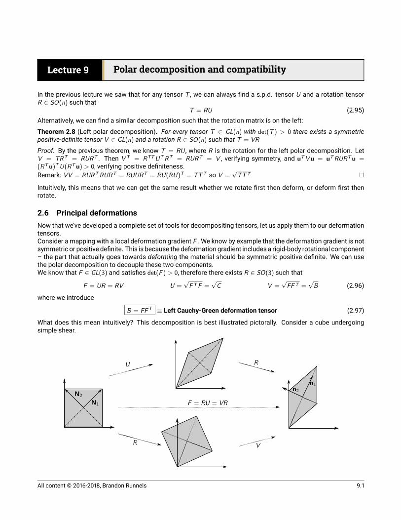
Lecture 9 Polar decomposition and compatibility
In the previous lecture we saw that for any tensor T , we can always find a s.p.d. tensor U and a rotation tensorR ∈ SO(n) such that
T = RU (2.95)Alternatively, we can find a similar decomposition such that the rotation matrix is on the left:Theorem 2.8 (Left polar decomposition). For every tensor T ∈ GL(n) with det(T ) > 0 there exists a symmetricpositive-definite tensor V ∈ GL(n) and a rotation R ∈ SO(n) such that T = VR
Proof. By the previous theorem, we know T = RU , where R is the rotation for the left polar decomposition. LetV = TRT = RURT . Then V T = RTTUTRT = RURT = V , verifying symmetry, and uTVu = uTRURTu =(RTu)TU(RTu) > 0, verifying positive definiteness.Remark: VV = RURTRURT = RUURT = RU(RU)T = TTT so V =
√TTT
Intuitively, this means that we can get the same result whether we rotate first then deform, or deform first thenrotate.2.6 Principal deformationsNow that we’ve developed a complete set of tools for decompositing tensors, let us apply them to our deformationtensors.Consider a mapping with a local deformation gradient F . We know by example that the deformation gradient is notsymmetric or positive definite. This is because the deformation gradient includes a rigid-body rotational component– the part that actually goes towards deforming the material should be symmetric positive definite. We can usethe polar decomposition to decouple these two components.We know that F ∈ GL(3) and satisfies det(F ) > 0, therefore there exists R ∈ SO(3) such that
F = UR = RV U =√FTF =
√C V =
√FFT =
√B (2.96)
where we introduceB = FFT ≡ Left Cauchy-Green deformation tensor (2.97)
What does this mean intuitively? This decomposition is best illustrated pictorally. Consider a cube undergoingsimple shear.
N1
N2
n1n2
U
R
R
V
F = RU = VR
All content © 2016-2018, Brandon Runnels 9.1
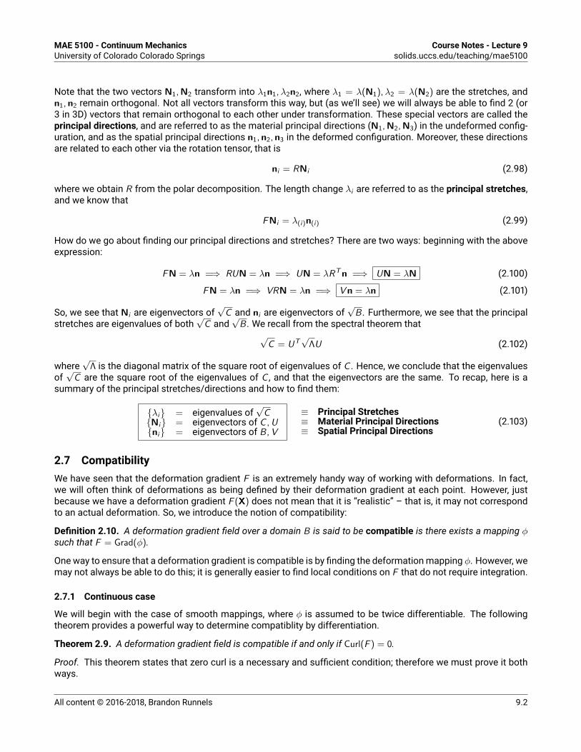
MAE 5100 - Continuum MechanicsUniversity of Colorado Colorado Springs Course Notes - Lecture 9solids.uccs.edu/teaching/mae5100
Note that the two vectors N1,N2 transform into λ1n1,λ2n2, where λ1 = λ(N1),λ2 = λ(N2) are the stretches, andn1,n2 remain orthogonal. Not all vectors transform this way, but (as we’ll see) we will always be able to find 2 (or3 in 3D) vectors that remain orthogonal to each other under transformation. These special vectors are called theprincipal directions, and are referred to as the material principal directions (N1,N2,N3) in the undeformed config-uration, and as the spatial principal directions n1,n2,n3 in the deformed configuration. Moreover, these directionsare related to each other via the rotation tensor, that is
ni = RNi (2.98)where we obtain R from the polar decomposition. The length change λi are referred to as the principal stretches,and we know that
FNi = λ(i)n(i) (2.99)How do we go about finding our principal directions and stretches? There are two ways: beginning with the aboveexpression:
FN = λn =⇒ RUN = λn =⇒ UN = λRTn =⇒ UN = λN (2.100)FN = λn =⇒ VRN = λn =⇒ Vn = λn (2.101)
So, we see that Ni are eigenvectors of √C and ni are eigenvectors of √B . Furthermore, we see that the principalstretches are eigenvalues of both√C and√B . We recall from the spectral theorem that√C = UT
√ΛU (2.102)
where √Λ is the diagonal matrix of the square root of eigenvalues of C . Hence, we conclude that the eigenvaluesof √C are the square root of the eigenvalues of C , and that the eigenvectors are the same. To recap, here is asummary of the principal stretches/directions and how to find them:λi = eigenvalues of√CNi = eigenvectors of C ,Uni = eigenvectors of B,V
≡ Principal Stretches≡ Material Principal Directions≡ Spatial Principal Directions
(2.103)
2.7 CompatibilityWe have seen that the deformation gradient F is an extremely handy way of working with deformations. In fact,we will often think of deformations as being defined by their deformation gradient at each point. However, justbecause we have a deformation gradient F (X) does not mean that it is “realistic” – that is, it may not correspondto an actual deformation. So, we introduce the notion of compatibility:Definition 2.10. A deformation gradient field over a domain B is said to be compatible is there exists a mapping φsuch that F = Grad(φ).
One way to ensure that a deformation gradient is compatible is by finding the deformationmapping φ. However, wemay not always be able to do this; it is generally easier to find local conditions on F that do not require integration.2.7.1 Continuous case
We will begin with the case of smooth mappings, where φ is assumed to be twice differentiable. The followingtheorem provides a powerful way to determine compatiblity by differentiation.Theorem 2.9. A deformation gradient field is compatible if and only if Curl(F ) = 0.
Proof. This theorem states that zero curl is a necessary and sufficient condition; therefore we must prove it bothways.All content © 2016-2018, Brandon Runnels 9.2
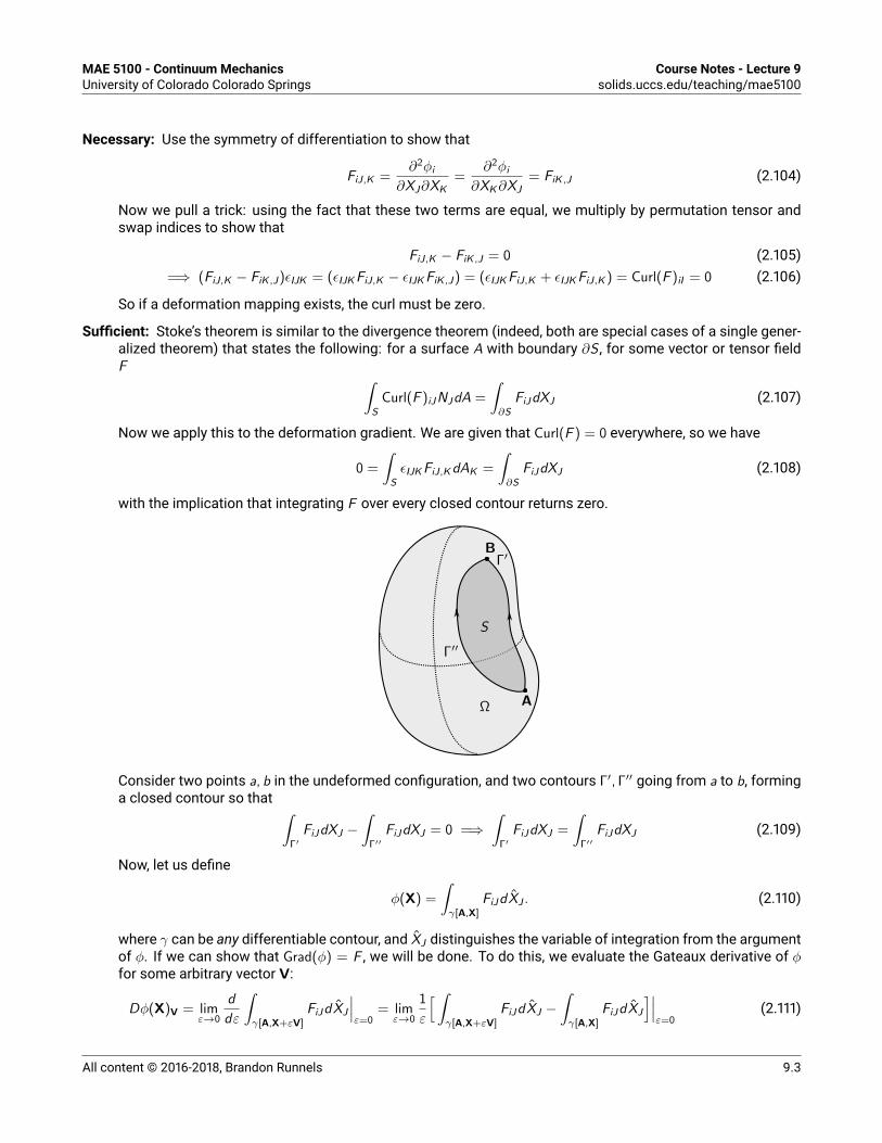
MAE 5100 - Continuum MechanicsUniversity of Colorado Colorado Springs Course Notes - Lecture 9solids.uccs.edu/teaching/mae5100
Necessary: Use the symmetry of differentiation to show thatFiJ,K =
∂2φi∂XJ∂XK
=∂2φi
∂XK∂XJ= FiK ,J (2.104)
Now we pull a trick: using the fact that these two terms are equal, we multiply by permutation tensor andswap indices to show thatFiJ,K − FiK ,J = 0 (2.105)
=⇒ (FiJ,K − FiK ,J)εIJK = (εIJKFiJ,K − εIJKFiK ,J) = (εIJKFiJ,K + εIJKFiJ,K ) = Curl(F )iI = 0 (2.106)So if a deformation mapping exists, the curl must be zero.
Sufficient: Stoke’s theorem is similar to the divergence theorem (indeed, both are special cases of a single gener-alized theorem) that states the following: for a surface A with boundary ∂S , for some vector or tensor fieldF ∫
S
Curl(F )iJNJdA =
∫∂S
FiJdXJ (2.107)Now we apply this to the deformation gradient. We are given that Curl(F ) = 0 everywhere, so we have
0 =
∫S
εIJKFiJ,KdAK =
∫∂S
FiJdXJ (2.108)with the implication that integrating F over every closed contour returns zero.
S
Γ′
Γ′′
Ω A
B
Consider two points a, b in the undeformed configuration, and two contours Γ′, Γ′′ going from a to b, forminga closed contour so that ∫Γ′FiJdXJ −
∫Γ′′
FiJdXJ = 0 =⇒∫
Γ′FiJdXJ =
∫Γ′′
FiJdXJ (2.109)Now, let us define
φ(X) =
∫γ[A,X]
FiJdXJ . (2.110)where γ can be any differentiable contour, and XJ distinguishes the variable of integration from the argumentof φ. If we can show that Grad(φ) = F , we will be done. To do this, we evaluate the Gateaux derivative of φfor some arbitrary vector V:Dφ(X)V = lim
ε→0
d
dε
∫γ[A,X+εV]
FiJdXJ
∣∣∣ε=0
= limε→0
1
ε
[ ∫γ[A,X+εV]
FiJdXJ −∫γ[A,X]
FiJdXJ
]∣∣∣ε=0
(2.111)
All content © 2016-2018, Brandon Runnels 9.3
MAE 5100 - Continuum MechanicsUniversity of Colorado Colorado Springs Course Notes - Lecture 9solids.uccs.edu/teaching/mae5100
Path independence allows us to break up the integral:= limε→0
1
ε
[ ∫γ[A,X]
FiJdXJ +
∫γ[X,εV]
FiJdXJ −∫γ[A,X]
FiJdXJ
]∣∣∣ε=0
=[
limε→0
1
ε
∫γ[X,εV]
FiJdXJ
]ε=0
(2.112)
Let γ[X,X + εV] be linear, and introduce the parameterization XI = XI + sVI , dXI = VIds :=[
limε→0
1
ε
∫ ε
0
FiJ(X + sV)VJds]ε=0
=[ d
dε
∫ ε
0
FiJ(X + sV)VJds]ε=0
=[FiJ(X + εV)VJ
]ε=0
(2.113)= FiJ(X)VJ (2.114)
whence we identify FiJ = Grad(φ), resulting from the fact that the above holds for all V.Thus the condition Curl(F ) = 0 is both necessary and sufficient for compatibility.This theorem is quite useful because we don’t always know if a deformation mapping exists. By this, we see thatwe only have to check that the curl is zero to ensure that it the deformation gradient for a real mapping.A notable exception/special case of this is dislocations. Dislocations introduce a discontinuity into the deformationmapping, and as such, they create a singularity. This means that the curl of the deformation gradient is nonzerowhenever there is a dislocation. In fact, we can actually use CurlF to determine the dislocation content of a sample.
All content © 2016-2018, Brandon Runnels 9.4
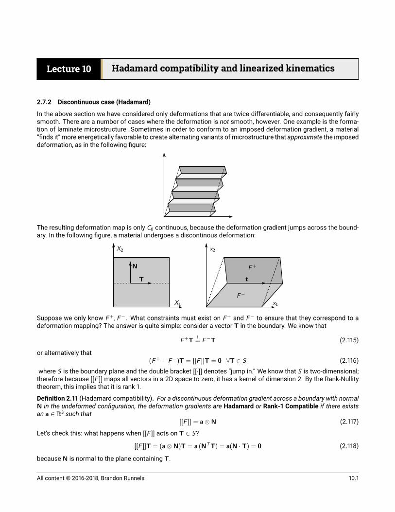
Lecture 10 Hadamard compatibility and linearized kinematics
2.7.2 Discontinuous case (Hadamard)
In the above section we have considered only deformations that are twice differentiable, and consequently fairlysmooth. There are a number of cases where the deformation is not smooth, however. One example is the forma-tion of laminate microstructure. Sometimes in order to conform to an imposed deformation gradient, a material“finds it”more energetically favorable to create alternating variants ofmicrostructure that approximate the imposeddeformation, as in the following figure:
The resulting deformation map is only C0 continuous, because the deformation gradient jumps across the bound-ary. In the following figure, a material undergoes a discontinous deformation:
T t
X1
X2
x1
x2
F+
F−
N
Suppose we only know F+,F−. What constraints must exist on F+ and F− to ensure that they correspond to adeformation mapping? The answer is quite simple: consider a vector T in the boundary. We know thatF+T
!= F−T (2.115)
or alternatively that(F+ − F−)T = [[F ]]T = 0 ∀T ∈ S (2.116)
where S is the boundary plane and the double bracket [[·]] denotes “jump in.” We know that S is two-dimensional;therefore because [[F ]] maps all vectors in a 2D space to zero, it has a kernel of dimension 2. By the Rank-Nullitytheorem, this implies that it is rank 1.Definition 2.11 (Hadamard compatibility). For a discontinuous deformation gradient across a boundary with normalN in the undeformed configuration, the deformation gradients are Hadamard or Rank-1 Compatible if there existsan a ∈ R3 such that
[[F ]] = a⊗N (2.117)Let’s check this: what happens when [[F ]] acts on T ∈ S?
[[F ]]T = (a⊗N)T = a (NTT) = a(N · T) = 0 (2.118)because N is normal to the plane containing T.All content © 2016-2018, Brandon Runnels 10.1
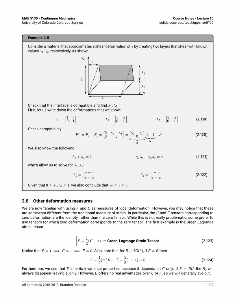
MAE 5100 - Continuum MechanicsUniversity of Colorado Colorado Springs Course Notes - Lecture 10solids.uccs.edu/teaching/mae5100
Example 2.5
Consider amaterial that approximates a shear deformation of γ by creating two layers that shearwith knownvalues γ1, γ2, respectively, as shown.
x1
x2
λ2
λ1
1
1
γ
Check that the interface is compatible and find λ1,λ2First, let us write down the deformations that we know:F =
[1 γ0 1
]F1 =
[1 γ10 1
]F2 =
[1 γ20 1
] (2.119)Check compatibility:
[[F ]] = F2 − F1 =[0 γ2 − γ10 0
]=[γ2 − γ1
0
]︸ ︷︷ ︸
a
[0 1]︸ ︷︷ ︸N
X (2.120)
We also know the followingλ1 + λ2 = 1 γ1λ1 + γ2λ2 = γ (2.121)
which allow us to solve for λ1,λ2:λ1 =
γ2 − γγ2 − γ1
λ2 =γ − γ1
γ2 − γ1(2.122)
Given that 0 ≤ λ1,λ2 ≤ 1, we also conclude that γ2 ≤ γ ≤ γ1
2.8 Other deformation measuresWe are now familiar with using F and C as measures of local deformation. However, you may notice that theseare somewhat different from the traditional measure of strain. In particular, the C and F tensors corresponding tozero deformation are the identity, rather than the zero tensor. While this is not really problematic, some prefer touse tensors for which zero deformation corresponds to the zero tensor. The first example is the Green-Lagrangestrain tensor:
E =1
2(C − I) ≡ Green-Lagrange Strain Tensor (2.123)
Notice that F = I =⇒ C = I =⇒ E = 0. Also, note that for R ∈ SO(3), if F = R thenE =
1
2(RTR − I) =
1
2(I− I) = 0 (2.124)
Furthermore, we see that E inherits invariance properties because it depends on C only: if F = RU , the R0 willalways disappear leaving U only. However, E offers no real advantages over C or F , so we will generally avoid it.All content © 2016-2018, Brandon Runnels 10.2
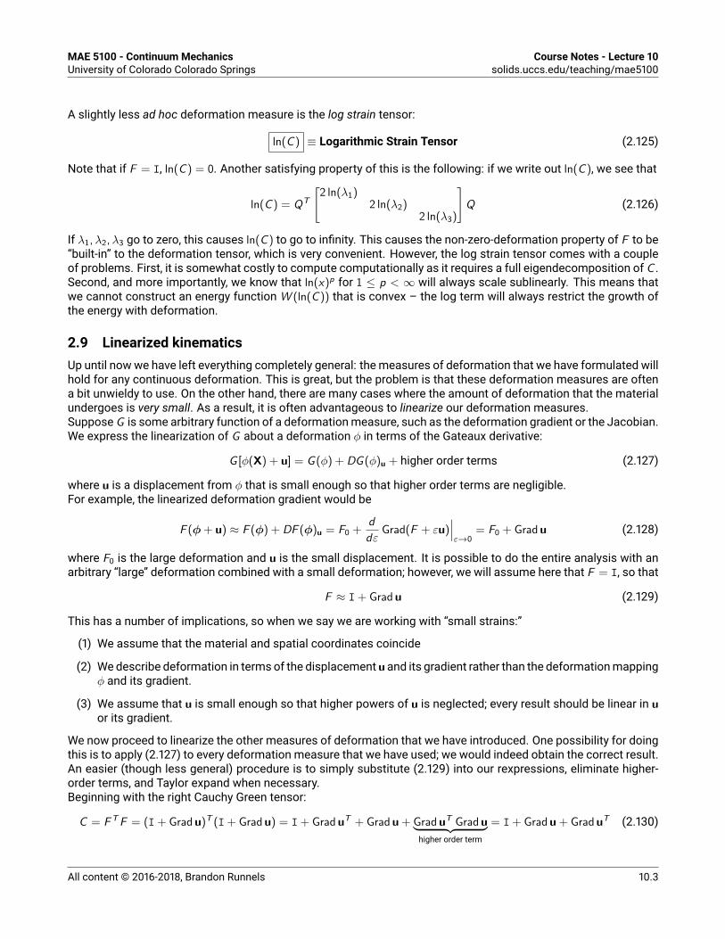
MAE 5100 - Continuum MechanicsUniversity of Colorado Colorado Springs Course Notes - Lecture 10solids.uccs.edu/teaching/mae5100
A slightly less ad hoc deformation measure is the log strain tensor:ln(C ) ≡ Logarithmic Strain Tensor (2.125)
Note that if F = I, ln(C ) = 0. Another satisfying property of this is the following: if we write out ln(C ), we see thatln(C ) = QT
[2 ln(λ1)
2 ln(λ2)2 ln(λ3)
]Q (2.126)
If λ1,λ2,λ3 go to zero, this causes ln(C ) to go to infinity. This causes the non-zero-deformation property of F to be“built-in” to the deformation tensor, which is very convenient. However, the log strain tensor comes with a coupleof problems. First, it is somewhat costly to compute computationally as it requires a full eigendecomposition of C .Second, and more importantly, we know that ln(x)p for 1 ≤ p < ∞ will always scale sublinearly. This means thatwe cannot construct an energy function W (ln(C )) that is convex – the log term will always restrict the growth ofthe energy with deformation.2.9 Linearized kinematicsUp until nowwe have left everything completely general: the measures of deformation that we have formulated willhold for any continuous deformation. This is great, but the problem is that these deformation measures are oftena bit unwieldy to use. On the other hand, there are many cases where the amount of deformation that the materialundergoes is very small. As a result, it is often advantageous to linearize our deformation measures.SupposeG is some arbitrary function of a deformationmeasure, such as the deformation gradient or the Jacobian.We express the linearization of G about a deformation φ in terms of the Gateaux derivative:
G [φ(X) + u] = G (φ) + DG (φ)u + higher order terms (2.127)where u is a displacement from φ that is small enough so that higher order terms are negligible.For example, the linearized deformation gradient would be
F (φ + u) ≈ F (φ) + DF (φ)u = F0 +d
dεGrad(F + εu)
∣∣∣ε→0
= F0 + Gradu (2.128)where F0 is the large deformation and u is the small displacement. It is possible to do the entire analysis with anarbitrary “large” deformation combined with a small deformation; however, we will assume here that F = I, so that
F ≈ I + Gradu (2.129)This has a number of implications, so when we say we are working with “small strains:”(1) We assume that the material and spatial coordinates coincide(2) We describe deformation in terms of the displacement u and its gradient rather than the deformationmapping
φ and its gradient.(3) We assume that u is small enough so that higher powers of u is neglected; every result should be linear in uor its gradient.
We now proceed to linearize the other measures of deformation that we have introduced. One possibility for doingthis is to apply (2.127) to every deformation measure that we have used; we would indeed obtain the correct result.An easier (though less general) procedure is to simply substitute (2.129) into our rexpressions, eliminate higher-order terms, and Taylor expand when necessary.Beginning with the right Cauchy Green tensor:C = FTF = (I + Gradu)T (I + Gradu) = I + GraduT + Gradu + GraduT Gradu︸ ︷︷ ︸
higher order term= I + Gradu + GraduT (2.130)
All content © 2016-2018, Brandon Runnels 10.3
MAE 5100 - Continuum MechanicsUniversity of Colorado Colorado Springs Course Notes - Lecture 10solids.uccs.edu/teaching/mae5100
Note that we drop out the GraduGraduT term because it is higher order in Gradu.Let us apply this to the Green-Lagrange strain tensor:E =
1
2(C − I) =
1
2(I + GraduT + Gradu− I) =
1
2(GraduT + Gradu) = sym(Gradu) (2.131)
i.e., E is the symmetric part of Gradu. It turns out that the linearized Green-Lagrange strain tensor is a very conve-nient choice for measuring deformation in small strains, and so it is given a special symbol:ε =
1
2(Gradu + GraduT ) ≡ Small Strain Tensor (2.132)
ε is symmetric, as we would expect. What about the antisymmetric part of Gradu? We definer =
1
2(Gradu− GraduT ) ≡ Infinitesimal Rotation Tensor (2.133)
The infinitesimal rotation tensor gives an indication of the rotation at a point, although it breaks down under largedeformation as does the small strain tensor. Note that ε + r = Gradu. This is actually the small-strain analog tothe polar decomposition. For future decompositions of F (such as the elastic-plastic decomposition) we will seethat the tensor-tensor multiplication in large strain boils down to a much friendlier additive decomposition in smallstrain.2.9.1 Linearized metric changes
What happens to our metric change measures when we apply linearization? Let’s begin by considering the stretch.Recalling our formula for λ(n) where n is the direction of stretch, and substituting our linearized measures ofdeformation, we getλ(n) =
√nTCn =
√nT (I + Gradu + GraduT )m =
√nTn + 2nT εn =
√1 + 2nT εn (2.134)
And now we’re stuck, because we have a nonlinear function of ε. But we know that ε is small, so we can apply alinearization of the square root function about 1:= 1 +
1
2(1 + 2nT εn− 1) = 1 + nT εn (2.135)
Rearranging this expression, we can write∆`
`0(n) = nT εn ≡ Engineering Strain (2.136)
Note that this implies that ε11 is the strain in the x1 direction, and so on; in other words, the diagonals of the smallstrain tensor describe the elongation in the x1, x2, x3 directions.
All content © 2016-2018, Brandon Runnels 10.4
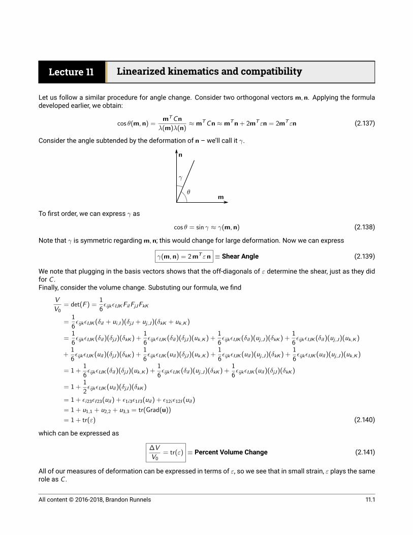
Lecture 11 Linearized kinematics and compatibility
Let us follow a similar procedure for angle change. Consider two orthogonal vectors m,n. Applying the formuladeveloped earlier, we obtain:cos θ(m,n) =
mTCn
λ(m)λ(n)≈ mTCn ≈ mTn + 2mT εn = 2mT εn (2.137)
Consider the angle subtended by the deformation of n – we’ll call it γ.
θ
γ
m
n
To first order, we can express γ ascos θ = sin γ ≈ γ(m,n) (2.138)
Note that γ is symmetric regarding m,n; this would change for large deformation. Now we can expressγ(m,n) = 2mT εn ≡ Shear Angle (2.139)
We note that plugging in the basis vectors shows that the off-diagonals of ε determine the shear, just as they didfor C .Finally, consider the volume change. Substuting our formula, we findV
V0= det(F ) =
1
6εijkεIJKFiIFjJFkK
=1
6εijkεIJK (δiI + ui ,I )(δjJ + uj ,J)(δkK + uk,K )
=1
6εijkεIJK (δiI )(δjJ)(δkK ) +
1
6εijkεIJK (δiI )(δjJ)(uk,K ) +
1
6εijkεIJK (δiI )(uj ,J)(δkK ) +
1
6εijkεIJK (δiI )(uj ,J)(uk,K )
+1
6εijkεIJK (uiI )(δjJ)(δkK ) +
1
6εijkεIJK (uiI )(δjJ)(uk,K ) +
1
6εijkεIJK (uiI )(uj ,J)(δkK ) +
1
6εijkεIJK (uiI )(uj ,J)(uk,K )
= 1 +1
6εijkεIJK (δiI )(δjJ)(uk,K ) +
1
6εijkεIJK (δiI )(uj ,J)(δkK ) +
1
6εijkεIJK (uiI )(δjJ)(δkK )
= 1 +1
2εijkεIJK (uiI )(δjJ)(δkK )
= 1 + εi23εI23(uiI ) + ε1i3ε1I3(uiI ) + ε12iε12I (uiI )
= 1 + u1,1 + u2,2 + u3,3 = tr(Grad(u))
= 1 + tr(ε) (2.140)which can be expressed as
∆V
V0= tr(ε) ≡ Percent Volume Change (2.141)
All of our measures of deformation can be expressed in terms of ε, so we see that in small strain, ε plays the samerole as C .All content © 2016-2018, Brandon Runnels 11.1
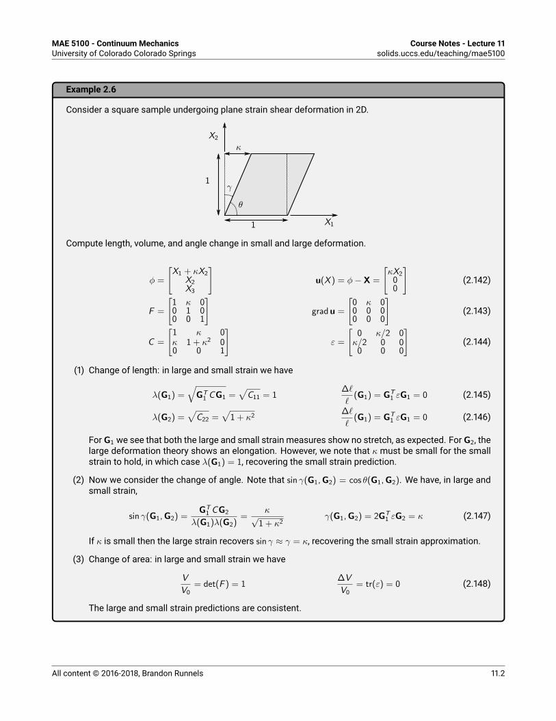
MAE 5100 - Continuum MechanicsUniversity of Colorado Colorado Springs Course Notes - Lecture 11solids.uccs.edu/teaching/mae5100
Example 2.6
Consider a square sample undergoing plane strain shear deformation in 2D.
κ
1
1
X1
X2
θ
γ
Compute length, volume, and angle change in small and large deformation.
φ =
[X1 + κX2
X2X3
]u(X ) = φ− X =
[κX2
00
](2.142)
F =
[1 κ 00 1 00 0 1
]gradu =
[0 κ 00 0 00 0 0
](2.143)
C =
[1 κ 0κ 1 + κ2 00 0 1
]ε =
[0 κ/2 0κ/2 0 0
0 0 0
](2.144)
(1) Change of length: in large and small strain we haveλ(G1) =
√GT
1 CG1 =√C11 = 1
∆`
`(G1) = GT
1 εG1 = 0 (2.145)λ(G2) =
√C22 =
√1 + κ2
∆`
`(G1) = GT
1 εG1 = 0 (2.146)ForG1 we see that both the large and small strain measures show no stretch, as expected. ForG2, thelarge deformation theory shows an elongation. However, we note that κ must be small for the smallstrain to hold, in which case λ(G1) = 1, recovering the small strain prediction.
(2) Now we consider the change of angle. Note that sin γ(G1,G2) = cos θ(G1,G2). We have, in large andsmall strain,sin γ(G1,G2) =
GT1 CG2
λ(G1)λ(G2)=
κ√1 + κ2
γ(G1,G2) = 2GT1 εG2 = κ (2.147)
If κ is small then the large strain recovers sin γ ≈ γ = κ, recovering the small strain approximation.(3) Change of area: in large and small strain we have
V
V0= det(F ) = 1
∆V
V0= tr(ε) = 0 (2.148)
The large and small strain predictions are consistent.
All content © 2016-2018, Brandon Runnels 11.2
MAE 5100 - Continuum MechanicsUniversity of Colorado Colorado Springs Course Notes - Lecture 11solids.uccs.edu/teaching/mae5100
2.9.2 Small strain compatibility
Consider the case of purely 2D strain. We know thatε11 = u1,1 ε12 = ε21 =
1
2(u1,2 + u2,1) ε22 = u2,2 (2.149)
Let us consider the following equation:ε11,22 − 2ε12,12 + ε22,11 = u1,122 − u1,212 − u2,112 + u2,211 (2.150)
Because of the symmetry of differentiation, we know that this equals= u1,122 − u1,122 − u2,211 + u2,211 = 0 (2.151)
As with large deformation, a strain field ε is said to be compatible if there exists a displacement field u such thatεij =
1
2(ui ,j + uj ,i ) (2.152)
As before, wemay only have a strain field without having a displacement field; verifying that (2.150) is equal to zerois a necessary and sufficient condition for 2D compatibility. In 3D, we have six such equationsε11,22 + ε22,11 − 2ε12,12 = 0 (2.153a)ε22,33 + ε33,22 − 2ε23,23 = 0 (2.153b)ε33,11 + ε11,33 − 2ε13,13 = 0 (2.153c)
ε11,23 + ε23,11 − ε31,21 − ε12,31 = 0 (2.153d)ε22,31 + ε23,12 − ε31,22 − ε12,32 = 0 (2.153e)ε33,12 + ε23,13 − ε31,23 − ε12,33 = 0 (2.153f)
We can alternatively express the above equations compactly ascurl curl ε = 0 (2.154)
which is necessary and sufficient for compatibility.2.10 The spatial/Eulerian pictureWe can use the machinery that we’ve developed for linearization to do something analagous. Consider some time-dependent deformation mapping φ(X, t), and some measure on φ, we’ll call it G [φ]. We can express the rate ofchange of G as the following derivative
G =∂
∂tG [φ(X, t)] = (gradG )
∂
∂tφ = (gradG )V = DGV. (2.155)
In other words, the time rate of change of G is nothing other than the Gateaux derivative of G in the direction of thevelocity V. This means that the procedure for deriving rates of G is exactly the same as deriving linearizations ofG . As such, we can dispense with the full derivation and jump directly to definition by analogy:Linearized kinematics Rates
Displacement ui Spatial velocity viDisplacement gradient βij = ui ,j Spatial velocity gradient `ij = vi ,jStrain tensor εij = 12 (βij + βji ) Rate of strain tensor dij = 1
2 (`ij + `ji )Infinitesimal rotation tensor rij = 12 (βij − βji ) Spin tensor wij = 1
2 (`ij − `ji )Rotation vector αk = 12 rjiεijk Vorticity vector ωij = 1
2wjiεijk
All content © 2016-2018, Brandon Runnels 11.3
MAE 5100 - Continuum MechanicsUniversity of Colorado Colorado Springs Course Notes - Lecture 11solids.uccs.edu/teaching/mae5100
Note that even though all of the above quantities are analagous to small strain deformation measures, we areno longer making the small strain approximation. We are merely showing that there are similarities between thelarge strain Eulerian rate quantities and the small strain linearized quantities. It is using these analogies that manyconnections are drawn between solid and fluid mechanics.As a side note, how do we relate these new large deformation measures to our familiar deformation measuressuch as F? The following identity is invaluable in expressing v , `, d ,w , etc., in terms of F :
FiIF−1Jj =
∂
∂t
( ∂xi∂XJ
)∂XJ
∂xj=
∂
∂XJ
(∂xi∂t
)∂XJ
∂xj=
∂vi∂XJ
∂XJ
∂xj=∂vi∂xj
= vi ,j = `ij (2.156)Written symbolically, we have the relationship
` = F F−1 (2.157)Let’s use the fact that we can draw analogies between small strain and rate deformation to derive the rate versionof metric changes. Beginning with volume change, we expect that
∆V
V= tr(ε) =⇒ V
V= tr(d) (2.158)
Let’s check to be sure. To do this, let us compute the derivative explicitly.J =
d
dtdet(F ) =
d(detF )
dFiJFiJ = (JF−TiJ )FiJ = J (FiJF
−1Ji ) = J tr(F F−1) = J tr(`) = J tr(d) (2.159)
Or, rearranging, we obtainJ
J=
V
V= tr(d) (2.160)
as expected. As a side note, we use the fact that tr(d) = dii = `ii = vi ,i = div(v) to obtain the useful identityJ = J div(v) (2.161)
This will come in handy when deriving time-dependent balance laws.Having verified that the analogy holds, we can use our small-strain derivations to construct rates ofmetric changes:• Rate of stretching: for a vector n the rate of change of its length is given by analogy to be
∆`
`(n) = nT εn =⇒
˙
`= nT d n (2.162)
• Rate of angle change: for two vectors m,n that are instantaneously orthogonal to each other, the rate ofchange of shear angle is given by analogy to beγ(m,n) = 2mT εn =⇒ γ(m,n) = 2mT d n (2.163)
Other rates of metric changes can be derived in a similar fashion.
All content © 2016-2018, Brandon Runnels 11.4
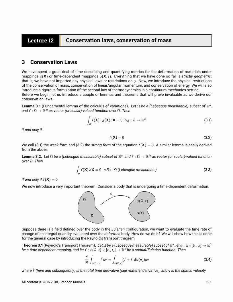
Lecture 12 Conservation laws, conservation of mass
3 Conservation LawsWe have spent a great deal of time describing and quantifying metrics for the deformation of materials undermappings φ(X) or time-dependent mappings φ(X, t). Everything that we have done so far is strictly geometric;that is, we have not imparted any physical laws or restrictions on φ. Now, we introduce the physical restrictionsof the conservation of mass, conservation of linear/angular momentum, and conservation of energy. We will alsointroduce a rigorous formulation of the second law of thermodynamics in a continuum mechanics setting.Before we begin, let us introduce a couple of lemmas and theorems that will prove invaluable as we derive ourconservation laws.Lemma 3.1 (Fundamental lemma of the calculus of variations). Let Ω be a (Lebesgue measurable) subset of Rn ,and f : Ω→ Rm as vector (or scalar)-valued function over Ω. Then∫
Ω
f (X) · g(X)dX = 0 ∀g : Ω→ Rm (3.1)if and only if
f (X) = 0 (3.2)We call (3.1) the weak form and (3.2) the strong form of the equation f (X) = 0. A similar lemma is easily derivedfrom the above:Lemma 3.2. Let Ω be a (Lebesgue measurable) subset of Rn , and f : Ω → Rm as vector (or scalar)-valued functionover Ω. Then ∫
B
f (X) dX = 0 ∀B ⊂ Ω (Lebesgue measurable) (3.3)if and only if f (X) = 0
We now introduce a very important theorem. Consider a body that is undergoing a time-dependent deformation.
Xx(t)
Ω φ(Ω, t)
φ
Suppose there is a field defined over the body in the Eulerian configuration, we want to evaluate the time rate ofchange of an integral quantity evaluated over the deformed body. How do we do it? We will show how this is donefor the general case by introducing the Reynold’s transport theorem:Theorem3.1 (Reynold’s Transport Theorem). Let Ω be a (Lebesguemeasurable) subset ofRn , letφ : Ω×[t1, t2]→ R3
be a time-dependent mapping, and let f : φ(Ω, t)× [t1, t2]→ Rn be a spatial/Eulerian function. Then
d
dt
∫φ(Ω,t)
f dv =
∫φ(Ω,t)
(f + f div(v))dv (3.4)where f (here and subsequently) is the total time derivative (see material derivative), and v is the spatial velocity.
All content © 2016-2018, Brandon Runnels 12.1

MAE 5100 - Continuum MechanicsUniversity of Colorado Colorado Springs Course Notes - Lecture 12solids.uccs.edu/teaching/mae5100
Proof. Let us begin by considering the left hand side:d
dt
∫φ(Ω,t)
f dv (3.5)We want to take the derivative inside the integral, but we can’t because the bound on the integral itself is time-dependent. To remedy this, we will perform a change of variables to evaluate the integral in the undeformed con-figuration. Then we have
φ(Ω, t)→ Ω dv = J dV (3.6)Our integral thus becomes
d
dt
∫Ω
f J dV =
∫Ω
d
dt(f J) dV (3.7)
We now evaluate the derivative using the product rule, and recalling (), we obtain=
∫Ω
(f J + f J) dV =
∫Ω
(f J + f J div(v)) dV =
∫Ω
(f + f div(v)) J dV (3.8)Changing variables back, we obtain
=
∫φ(Ω,t)
(f + f div(v)) dv (3.9)concluding the proof.With this machinery in hand, we will now proceed to derive balance laws.3.1 Conservation of MassTo develop conservation of mass, we must introduce two new quantities:
R(X, t) ≡ Lagrangian Mass Density ρ(x, t) ≡ Eulerian Mass Density (3.10)The Lagrangian mass density is the mass per unit undeformed volume and is defined in the undeformed config-uration, whereas the Eulerian mass density is the mass per unit deformed volume and is defined in the deformedconfiguration. We can relate the two in the following way:
R =dm
dV=
dm
dv/J= J
dm
dv= J ρ (3.11)
Furthermore, for a region B ⊂ Ω contained in the body, we can express the total mass in that body asm(B) =
∫B
R dV =
∫φ(B,t)
ρ dv (3.12)Now, we introduce mass conservation by stating that for every B ⊂ Ω (measurable) and for all time,
d
dtm(B) = 0 (3.13)
Pictorally, consider a body that is undergoing a deformation as follows:
All content © 2016-2018, Brandon Runnels 12.2
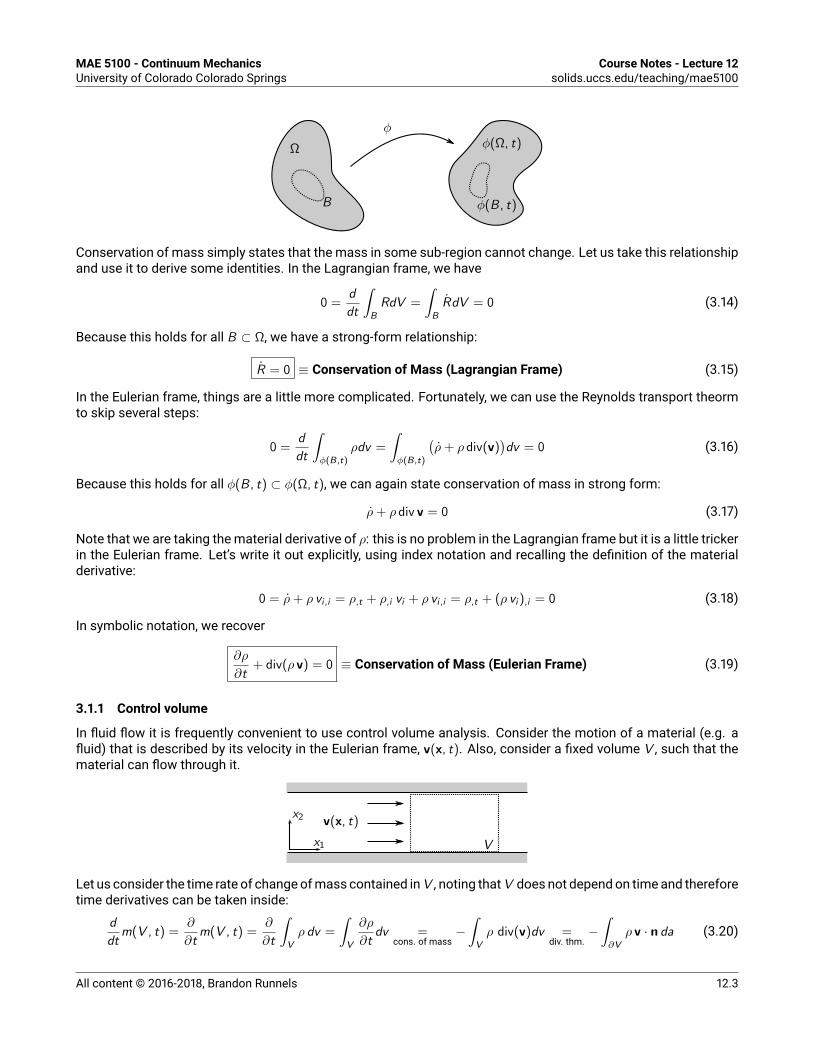
MAE 5100 - Continuum MechanicsUniversity of Colorado Colorado Springs Course Notes - Lecture 12solids.uccs.edu/teaching/mae5100
Ω φ(Ω, t)φ
B φ(B, t)
Conservation of mass simply states that the mass in some sub-region cannot change. Let us take this relationshipand use it to derive some identities. In the Lagrangian frame, we have0 =
d
dt
∫B
RdV =
∫B
RdV = 0 (3.14)Because this holds for all B ⊂ Ω, we have a strong-form relationship:
R = 0 ≡ Conservation of Mass (Lagrangian Frame) (3.15)In the Eulerian frame, things are a little more complicated. Fortunately, we can use the Reynolds transport theormto skip several steps:
0 =d
dt
∫φ(B,t)
ρdv =
∫φ(B,t)
(ρ+ ρ div(v)
)dv = 0 (3.16)
Because this holds for all φ(B, t) ⊂ φ(Ω, t), we can again state conservation of mass in strong form:ρ+ ρ div v = 0 (3.17)
Note that we are taking thematerial derivative of ρ: this is no problem in the Lagrangian frame but it is a little trickerin the Eulerian frame. Let’s write it out explicitly, using index notation and recalling the definition of the materialderivative:0 = ρ+ ρ vi ,i = ρ,t + ρ,i vi + ρ vi ,i = ρ,t + (ρ vi ),i = 0 (3.18)
In symbolic notation, we recover∂ρ
∂t+ div(ρ v) = 0 ≡ Conservation of Mass (Eulerian Frame) (3.19)
3.1.1 Control volume
In fluid flow it is frequently convenient to use control volume analysis. Consider the motion of a material (e.g. afluid) that is described by its velocity in the Eulerian frame, v(x, t). Also, consider a fixed volume V , such that thematerial can flow through it.
v(x, t)
Vx1
x2
Let us consider the time rate of change ofmass contained inV , noting thatV does not dependon time and thereforetime derivatives can be taken inside:d
dtm(V , t) =
∂
∂tm(V , t) =
∂
∂t
∫V
ρ dv =
∫V
∂ρ
∂tdv =cons. of mass −
∫V
ρ div(v)dv =div. thm. −∫∂V
ρ v · n da (3.20)
All content © 2016-2018, Brandon Runnels 12.3
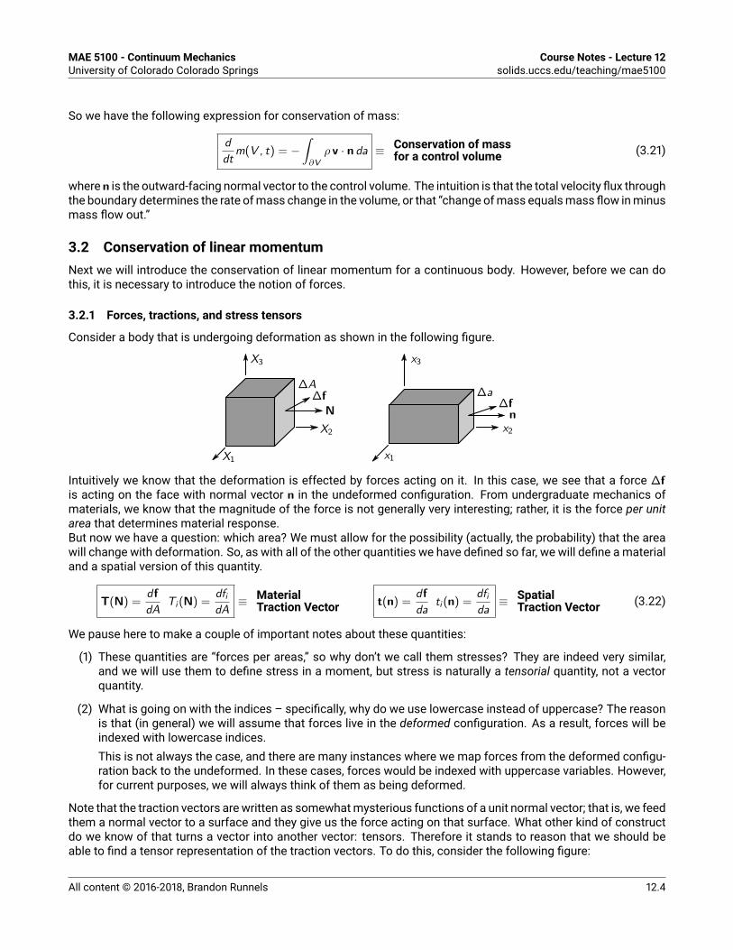
MAE 5100 - Continuum MechanicsUniversity of Colorado Colorado Springs Course Notes - Lecture 12solids.uccs.edu/teaching/mae5100
So we have the following expression for conservation of mass:d
dtm(V , t) = −
∫∂V
ρ v · n da ≡ Conservation of massfor a control volume (3.21)
where n is the outward-facing normal vector to the control volume. The intuition is that the total velocity flux throughthe boundary determines the rate ofmass change in the volume, or that “change ofmass equalsmass flow inminusmass flow out.”3.2 Conservation of linear momentumNext we will introduce the conservation of linear momentum for a continuous body. However, before we can dothis, it is necessary to introduce the notion of forces.3.2.1 Forces, tractions, and stress tensors
Consider a body that is undergoing deformation as shown in the following figure.
N n
∆A∆a
X1
X2
X3
x1
x2
x3
∆f∆f
Intuitively we know that the deformation is effected by forces acting on it. In this case, we see that a force ∆fis acting on the face with normal vector n in the undeformed configuration. From undergraduate mechanics ofmaterials, we know that the magnitude of the force is not generally very interesting; rather, it is the force per unitarea that determines material response.But now we have a question: which area? We must allow for the possibility (actually, the probability) that the areawill change with deformation. So, as with all of the other quantities we have defined so far, we will define amaterialand a spatial version of this quantity.
T(N) =df
dATi (N) =
dfidA≡ Material
Traction Vector t(n) =df
dati (n) =
dfida≡ Spatial
Traction Vector (3.22)We pause here to make a couple of important notes about these quantities:(1) These quantities are “forces per areas,” so why don’t we call them stresses? They are indeed very similar,and we will use them to define stress in a moment, but stress is naturally a tensorial quantity, not a vectorquantity.(2) What is going on with the indices – specifically, why do we use lowercase instead of uppercase? The reasonis that (in general) we will assume that forces live in the deformed configuration. As a result, forces will beindexed with lowercase indices.
This is not always the case, and there are many instances where we map forces from the deformed configu-ration back to the undeformed. In these cases, forces would be indexed with uppercase variables. However,for current purposes, we will always think of them as being deformed.Note that the traction vectors arewritten as somewhatmysterious functions of a unit normal vector; that is, we feedthem a normal vector to a surface and they give us the force acting on that surface. What other kind of constructdo we know of that turns a vector into another vector: tensors. Therefore it stands to reason that we should beable to find a tensor representation of the traction vectors. To do this, consider the following figure:All content © 2016-2018, Brandon Runnels 12.4
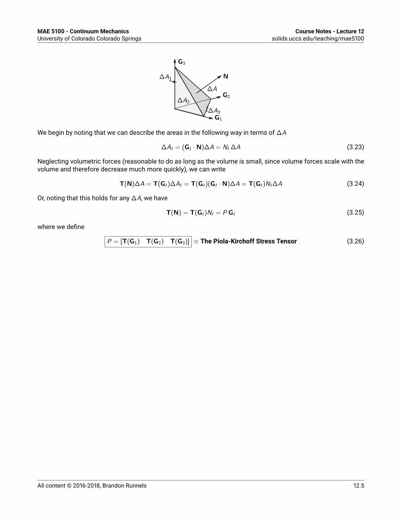
MAE 5100 - Continuum MechanicsUniversity of Colorado Colorado Springs Course Notes - Lecture 12solids.uccs.edu/teaching/mae5100
N
∆A
∆A1
∆A2
∆A3
G1
G2
G3
We begin by noting that we can describe the areas in the following way in terms of ∆A
∆AI = (GI ·N)∆A = NI ∆A (3.23)Neglecting volumetric forces (reasonable to do as long as the volume is small, since volume forces scale with thevolume and therefore decrease much more quickly), we can write
T(N)∆A = T(GI )∆AI = T(GI )(GI ·N)∆A = T(GI )NI∆A (3.24)Or, noting that this holds for any ∆A, we have
T(N) = T(GI )NI = P GI (3.25)where we define
P = [T(G1) T(G2) T(G3)] ≡ The Piola-Kirchoff Stress Tensor (3.26)
All content © 2016-2018, Brandon Runnels 12.5
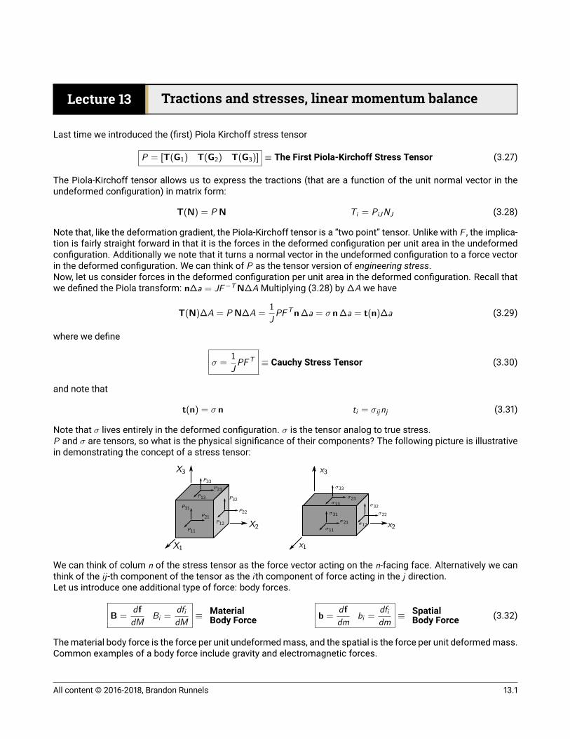
Lecture 13 Tractions and stresses, linear momentum balance
Last time we introduced the (first) Piola Kirchoff stress tensorP = [T(G1) T(G2) T(G3)] ≡ The First Piola-Kirchoff Stress Tensor (3.27)
The Piola-Kirchoff tensor allows us to express the tractions (that are a function of the unit normal vector in theundeformed configuration) in matrix form:T(N) = P N Ti = PiJNJ (3.28)
Note that, like the deformation gradient, the Piola-Kirchoff tensor is a “two point” tensor. Unlike with F , the implica-tion is fairly straight forward in that it is the forces in the deformed configuration per unit area in the undeformedconfiguration. Additionally we note that it turns a normal vector in the undeformed configuration to a force vectorin the deformed configuration. We can think of P as the tensor version of engineering stress.Now, let us consider forces in the deformed configuration per unit area in the deformed configuration. Recall thatwe defined the Piola transform: n∆a = JF−TN∆A Multiplying (3.28) by ∆A we haveT(N)∆A = P N∆A =
1
JPFTn∆a = σ n∆a = t(n)∆a (3.29)
where we defineσ =
1
JPFT ≡ Cauchy Stress Tensor (3.30)
and note thatt(n) = σ n ti = σijnj (3.31)
Note that σ lives entirely in the deformed configuration. σ is the tensor analog to true stress.P and σ are tensors, so what is the physical significance of their components? The following picture is illustrativein demonstrating the concept of a stress tensor:
P22
X1
X2
X3
x1
x3
P32
P12
P11
P21
P31
P33
P23
P13
σ33
σ23σ13
σ31
σ21
σ11
σ32
σ22
σ12 x2
We can think of colum n of the stress tensor as the force vector acting on the n-facing face. Alternatively we canthink of the ij -th component of the tensor as the ith component of force acting in the j direction.Let us introduce one additional type of force: body forces.B =
df
dMBi =
dfidM
≡ MaterialBody Force b =
df
dmbi =
dfidm
≡ SpatialBody Force (3.32)
Thematerial body force is the force per unit undeformedmass, and the spatial is the force per unit deformedmass.Common examples of a body force include gravity and electromagnetic forces.
All content © 2016-2018, Brandon Runnels 13.1
MAE 5100 - Continuum MechanicsUniversity of Colorado Colorado Springs Course Notes - Lecture 13solids.uccs.edu/teaching/mae5100
3.2.2 Balance laws
Recall that momentum is mass times velocity. What is momentum for a body with variable density R(X, t), ρ(x, t)and variable velocity V(X, t), v(x, t)? We can write it in integral form in either the material or spatial frames asL(B, t) =
∫B
R V dV =
∫φ(B,t)
ρ v dv (3.33)We can express Newton’s second law, the conservation of linear momentum, for all B ⊂ Ω as
d
dtL(B, t) = F(B, t) (3.34)
where F is the resultant of all forces acting on or in B ⊂ Ω,F(B, t) =
∫∂B
T (N)dA +
∫B
R B dV =
∫φ(∂B,t)
t(n)da +
∫B
ρb dv (3.35)Let us begin by considering the conservation of linear momentum in the Lagrangian frame only: we have
d
dt
∫B
R V dV =
∫∂B
T (N)dA +
∫B
R B dV (3.36)What do we do with the partial derivative? We can take it right inside the integral.
d
dt
∫B
R V dV =
∫B
d
dt(R V) dV =
∫B
(0
R V + R V) dV =
∫B
R A dV (3.37)Now, let’s consider the right hand side. In particular, let’s consider the surface traction term. Because we can writethe surface traction term as a matrix-vector multiplication with the Piola-Kirchoff stress tensor, we can apply thedivergence theorem to get ∫
∂B
T (N)dA =
∫∂B
P NdA =
∫B
Div(P)dV (3.38)Note that we now have three volume integrals. We can use this to collect terms andwrite our conservation equationas ∫
B
[R A− Div(P)− R B] dV = 0 (3.39)Because this must hold true for all B ⊂ Ω, applying the fundamental lemma of the Calculus of Variations, we canwrite the above in strong form:
Div(P) + RB = RAPiJ,J + R Bi = R Ai
≡ Conservation of Linear Momentum (Lagrangian Frame) (3.40)Now, let us consider the Eulerian frame:
d
dt
∫φ(B,t)
ρ v dv =
∫φ(∂B,t)
t(n)da +
∫B
ρb dv (3.41)As before, let us consider the left hand quantity first. In a similar procedure to that which we followed with conser-vation of mass, we apply the Reynold’s Transport Theorem to take the derivative inside the integral:
d
dt
∫φ(B,t)
ρ v dv =
∫φ(B,t)
[ ddt
(ρ v) + ρ v div(v)]dv =
∫φ(B,t)
[ρv + ρ v + ρ v div(v)]dv (3.42)=
∫φ(B,t)
[ρ v + v(:
0ρ+ ρ div(v))︸ ︷︷ ︸
conservation of mass]dv =
∫φ(B,t)
ρ a dv (3.43)
All content © 2016-2018, Brandon Runnels 13.2
MAE 5100 - Continuum MechanicsUniversity of Colorado Colorado Springs Course Notes - Lecture 13solids.uccs.edu/teaching/mae5100
Now, let us consider the surface tractions term on the right hand side. Again, we can apply the divergence theoremto obtain ∫φ(∂B,t)
t(n)da =
∫φ(∂B,t)
σ n da =
∫φ(B,t)
div(σ) dv (3.44)Combining all of the terms, which are now in integral form, we have∫
φ(B,t)
[ρa− div(σ)− ρb] dv = 0 (3.45)By the fundamental lemma, we can write the above in strong form as
div(σ) + ρb = ρaσij ,j + ρ bi = ρai
≡ Conservation of Linear Momentum (Eulerian Frame) (3.46)The above form for linear momentum balance is convenient for solid mechanics, but it can easily be rewritten in anumber of ways. A particularly popluar method (especially when doing fluid mechanics) is to start by writing thetime derivative in a different way:
d
dt(ρ vi ) + ρ vi vj ,j =
∂
∂t(ρ vi ) +
∂
∂xj(ρ vi )vj + ρ vi vj ,j =
∂
∂t(ρ vi ) +
∂
∂xj(ρ vi vj) (3.47)
In symbolic form, this can be expressed as∂
∂t(ρ v) + div(ρv ⊗ v) (3.48)
The Cauchy stress tensor is frequently decomposed into two components: a hydrostatic pressure component anda deviatoric stress component:σ = −pI + τ (3.49)
where p is the scalar hydrostatic pressure, and is negative because pressure is compressive. Finally, make theassumption that the only body force is gravity. Making all of these substitutions and rearranging a bit, the balanceof linear momentum can be expressed in the following form:∂
∂t(ρv) + div(ρv ⊗ v + pI) = div(τ) + ρ g ≡ Navier-Stokes Momentum Equation (3.50)
Even though the equation looks quite different, the mechanics are still the same. The biggest simplification madewhen writing the Navier-Stokes equations is in decoupling the stress tensor. Solid bodies are capable of sustainingstress states that are much more complex than that sustained by fluids, so we will prefer to leave σ in its non-decoupled form.
All content © 2016-2018, Brandon Runnels 13.3
Lecture 14 Conservation of angular momentum, energy
3.3 Conservation of angular momentumAngular momentum for a body B ⊂ Ω is given y
G =
∫B
x× RV dV =
∫φ(B,t)
x× ρv dv (3.51)and the moments generated from the applied body forces and surface tractions are
M =
∫∂B
x× T(N) dA +
∫B
x× R B dv =
∫φ(∂B,t)
x× t(n) da +
∫φ(B,t)
x× ρb dv (3.52)We note the important fact that we use the spatial position x for both the Lagrangian and Eulerian formulation. Thisis a result of the fact that our forces live in the deformed configuration, so the moments generated by them mustalso live in the deformed configuration.Having defined angular momentum and moments for a continuous body, we can now express the conservation ofangular momentum as
d
dtG(B, t) = M(B, t) (3.53)
Let us begin with the Lagrangian frame. We start by simplifying the time derivative, which is easy here as it is takenright inside the integral. Using the product rule, noting thatV×V = 0, and applying conservation of mass, we arriveat the expressiond
dt
∫B
x× RVdV =
∫B
[( x=V× RV) + (x×
0
RV) + (x× RV)]dV =
∫B
x× RAdV (3.54)As with linear momentum balance, we want to attempt to write the surface integral in volume form. The presenceof the cross product makes the application of the divergence theorem tricky, so we will switch to index notationhere. Applying the divergence theorem and the product rule, and applying the previously obtained conservation ofmomentum equation, we have∫
∂B
[x× T(N)]k dA =
∫∂B
[x× P N]k dA =
∫∂B
εijkxiPjPNP dA =
∫B
(εijkxiPjP),P dV (3.55)=
∫B
(εijk xi ,P︸︷︷︸FiP
PjP + εijkxiPjP,P︸ ︷︷ ︸[x×Div P]K
) dV =
∫B
(εijkFiPPjP + [x× (RA− RB)]k) dV (3.56)
Combining the above we have∫B
[x× RA]kdV︸ ︷︷ ︸momentum derivative
=
∫B
[εijkFiPPjP + [x× (RA− RB)]kdv︸ ︷︷ ︸
surface tractions+
∫B
[X× R B]kdV︸ ︷︷ ︸body force
(3.57)
Almost everything cancels except for one term. Because this holds ∀B ⊂ Ω, we can write the remaining term instrong form:εijkFiPP
TPj = 0 (3.58)
All content © 2016-2018, Brandon Runnels 14.1
MAE 5100 - Continuum MechanicsUniversity of Colorado Colorado Springs Course Notes - Lecture 14solids.uccs.edu/teaching/mae5100
We can now pull an index notation trick to simplify the above even further:0 = εijkFiPP
TPj =
1
2(εijkFiPP
TPj + εijkFiPP
TPj) =swap indices
1
2(εijkFiPP
TPj − εjikFiPP
TPj) (3.59)
=rename1
2(εijkFiPP
TPj − εijkFjPP
TPi ) =
1
2εijk(FiPP
TPj − PiPF
TPj) = 0 (3.60)
We see that this impliesFPT = PFT ≡ Conservation of Angular Momentum (Lagrangian Frame) (3.61)
All content © 2016-2018, Brandon Runnels 14.2
Lecture 15 Conservation of angular momentum, energy
Now let us consider the spatial frame. As before, we begin by using the transport theorem to simplify the timederivative term. We also apply the product rule and conservation of mass, arriving at:d
dt
∫φ(B,t)
x× ρv dv =
∫φ(B,t)
[ ddt
(x× ρv) + (x× ρv) div(v)]dv (3.62)
=
∫φ(B,t)
[(x× ρv) + (x× ρv) + (x× ρv) + (x× ρv) div(v)
]dv (3.63)
=
∫φ(B,t)
[
:0( x
=v× ρv) + (x× ρv) + (x× v) [
:0
ρ+ ρ div(v)]︸ ︷︷ ︸Mass conservation
]dv (3.64)
=
∫φ(B,t)
x× ρa dv (3.65)Now let’s look at the appliedmoment terms. In particular, we want to try to apply the divergence theorem to convertthe surface term to a volume term: Again, we’ll find that it is much easier to use index notation here.[ ∫
φ(∂B,t)
x× t(n) da]k
=[ ∫
φ(∂B,t)
x× σn da]k
=
∫φ(∂B,t)
εijkxiσjpnp da =
∫φ(B,t)
∂
∂xp(εijkxiσjp) dv (3.66)
=
∫φ(B,t)
(εijk xi ,p︸︷︷︸δip
σjp + εijkxiσjp,p) dv =
∫φ(B,t)
(εijkσji + [x× div σ]k) dv (3.67)
=
∫φ(B,t)
(εijkσji + [x× (ρa− ρb)]k) dv (3.68)Combining all of the terms in the conservation equation, we obtain∫
φ(B,t)
[x× ρa]k dv︸ ︷︷ ︸momentum rate
=
∫φ(B,t)
(εijkσji + [x× (ρa− ρb)]k)dv︸ ︷︷ ︸surface tractions
+
∫φ(B,t)
[x× ρb]k dv︸ ︷︷ ︸body forces
(3.69)
Now we see that almost everything cancels except for one term:∫φ(B,t)
εijkσjidv = 0 (3.70)Because this holds for all B , we can write it locally as
εijkσji = 0 (3.71)Using a procedure identical to the above, we arrive at the following expression for conservation of angular momen-tum:
σ = σT ≡ Conservation of Angular Momentum (Eulerian Frame) (3.72)Recalling the relationship between P and σ, we note that this is consistent with the Eulerian frame.3.4 Conservation of energyWe have established continuum mechanical formulations of the conservation of mass, linear momentum, andangular momentum. The final conservation law is the conservation of energy. Energy conservation is interestingbecause it is where we begin to make connections with other mechanisms such as mass or thermal transport. Infact, it is the great strength of energy conservation that almost all mechanisms have an energetic formulation thatallows the coupling of these phenomena together.All content © 2016-2018, Brandon Runnels 15.1
MAE 5100 - Continuum MechanicsUniversity of Colorado Colorado Springs Course Notes - Lecture 15solids.uccs.edu/teaching/mae5100
Before we begin, let us remind ourselves of a couple of important thermodynamical definitions:Definition 3.1. An extensive quantity for a system is a quantity that is equal to the sum of the quantities of allsubsystems. (Defined in integral form – a “nonlocal” quantity.)
Definition 3.2. An intensive quantity for a system is a quantity whose value is independent of the subsystem con-taining it. (Defined pointwise – a “local” quantity.)
3.4.1 Energetic quantities
To describe our energetic conservation laws, we need to make some definitions. Some are familiar, while somerequire the definition of new quantities.• Kinetic energy: kinetic energy for a body Ω is an extensive quantity, given by an integral over the entire volume.We recall that the kinetic energy for a particle is 1
2mv2. For a body with variable density and with variableinternal speed, the total kinetic energy isK (Ω) =
1
2
∫Ω
R||V||2dV =1
2
∫φ(Ω)
ρ||v||2dv ≡ Kinetic Energy (3.73)(We note that V, v are mean velocities, not velocities due to thermal fluctuations. We can do this becausewe are working at the continuum level and we will account for thermal fluctuations with temperature. Note,this is a little trickier with turbulent fluids, because fluctuations on the continuum level transfer down to themicroscopic level; this is called the energy cascade.)
• Heat: we have not dealt with heat yet, so in order to quantify it in a continuum setting we need to introduce acouple of new variables. Q(Ω) denotes the total heat of the body, with Ω representing the rate of change ofheat. We define Sn(X), sn(x) to be the heat generated in the material per unit undeformed mass and per unitdeformed mass, respectively. Finally, we let H,h be the heat flux vectors per unit deformed area and per unitundeformed area, respectively. With these definitions, we can write a simple heat balance law for our body inboth the Lagrangian and Eulerian configurations:Q(Ω) =
∫Ω
R Sn dV︸ ︷︷ ︸internal generation
−∫∂Ω
H ·N dA︸ ︷︷ ︸outward flux
=
∫φ(Ω)
ρ sn dv −∫φ(∂Ω)
h · n da (3.74)
We note that the divergence theorem allows us also to writeQ(Ω) =
∫Ω
[R Sn − Div(H)] dV =
∫φ(Ω)
[ρ sn − div(h)]dv (3.75)This is not of much use to us yet, because we have no relationship between these variables and the variablesthat we are using for everything else (P,F , etc.). However it will be useful when we construct our energybalance law.
• External power: we define the external power to be the rate of work done by all external forces. Rememberthat work done by a force is f ·∆x, so the power exerted by a force is f · v. Therefore, to capture the powerof the applied body forces and surface tractions, we dot them with the velocity of the material at the point ofapplication, then integrate over the body:PE (Ω) =
∫Ω
RB · VdV︸ ︷︷ ︸power of body forces
+
∫∂Ω
T(N) · VdA︸ ︷︷ ︸power of surface tractions
=
∫φ(Ω)
ρb · vdv +
∫φ(∂Ω)
t(n) · vda (3.76)
All content © 2016-2018, Brandon Runnels 15.2
Lecture 16 Conservation of energy, second law
• Deformation power: the deformation power is the portion of the external power that goes towards deformingthe material, rather than going towards changing the kinetic energy. For instance, if you throw a football, yourapplied surface tractions cause the football to start moving; on the other hand, if you squeeze the football,the kinetic energy doesn’t change (much) so all of your energy goes into deforming the ball. This quantity isactually defined rather easily as the difference between external power and change in kinetic energy:PD(Ω) = PE (Ω)− K (Ω)
=
∫Ω
RBiVidV +
∫∂Ω
ViPiJNJdA−1
2
d
dt
∫Ω
RViVidV (3.77)
=
∫Ω
RBiVidV +
∫Ω
(ViPiJ),JdV −1
2
∫Ω
[0 conservation of mass
RViVi + 2RViAi ]dV
=
∫Ω
[RBiVi + Vi ,JPiJ + ViPiJ,J − RViAi
]dV =
∫Ω
[Vi ,J︸︷︷︸=FiJ
PiJ + Vi
:0
(RBi + PiJ,J − RAi )︸ ︷︷ ︸conservation of momentum
]dV
=
∫Ω
FiJPiJdV =
∫Ω
F · P dV (3.78)(Note that the · symbol between two tensorsis used to indicate a termwise product, so that the result is ascalar.) Now let us, as usual, do the same thing in the Eulerian configuration:
PD(Ω) =
∫φ(Ω)
ρbividv +
∫φ(∂Ω)
viσijnjda−1
2
d
dt
∫φ(Ω)
ρvividv
=
∫φ(Ω)
ρbividv +
∫φ(Ω)
(viσij),jdv −1
2
∫φ(Ω)
(2ρviai +
:0
ρvivi + ρvivivj ,j︸ ︷︷ ︸conservation of mass
)dv
=
∫φ(Ω)
[
:0
ρbivi − ρviai + viσij ,j︸ ︷︷ ︸conservation of momentum
+ vi ,j︸︷︷︸=dij
σij ]dv
=
∫φ(Ω)
dijσijdv =
∫φ(Ω)
d · σ dv (3.79)where we recall that d was the rate of strain tensor. So, we can now write
PD(Ω) =
∫Ω
F · P dV =
∫φ(Ω)
d · σ dv ≡ Deformation Power (3.80)• Internal Energy: let us define the intensive variables U(X) and u(x), the internal energies per unit undeformedmass and deformed mass, respectively. Then the internal energy of a body Ω is given by
E (Ω) =
∫Ω
R U dV =
∫φ(Ω)
ρ u dv ≡ Internal Energy (3.81)3.4.2 Balance laws
We are now in a position to write the first law of thermodynamics in a continuum mechanics setting. We will stateit as:[change in internal energy] + [change in kinetic energy] = [external power] + [heat flow & generation] (3.82)
All content © 2016-2018, Brandon Runnels 16.1
MAE 5100 - Continuum MechanicsUniversity of Colorado Colorado Springs Course Notes - Lecture 16solids.uccs.edu/teaching/mae5100
Using what we have developed above, we writeE (Ω) + K (Ω) = PE (Ω) + Q(Ω) ≡ Conservation of Energy (3.83)
for all Ω. Alternatively, using our definition of deformation power, we can writeE (Ω) = PD(Ω) + Q(Ω) (3.84)
Since we have a nice and compact form for PD , the above expression is a little more useful. We already haveexpressions for PD and Q in Lagrangian and Eulerian forms, nowwe just need to evaluate E . Hopefully this processis starting to seem fairly familiar: in the Lagrangian form,
E (Ω) =d
dt
∫Ω
R U dV =
∫Ω
[0
R U + R U]dV =
∫Ω
R U dV (3.85)In the Eulerian form
E (Ω) =d
dt
∫φ(Ω)
ρ u dv =
∫φ(Ω)
[ρu +
:0
ρ u + ρ u div(v)︸ ︷︷ ︸conservation of mass
] dv =
∫φ(Ω)
ρ u dv (3.86)
Now, putting it all together, we have in the material/Lagrangian and spatial/Eulerian frames:∫Ω
R U dV =
∫Ω
F · P dV +
∫Ω
[R Sn − Div(H)] dV (3.87)∫φ(Ω)
ρ u dv =
∫φ(Ω)
d · σ dv +
∫φ(Ω)
[ρ sn − div(h)]dv (3.88)By the fundamental lemma, since the above holds for all subbodies Ω, we can finally write the above locally as
R U = F · P + R Sn − Div(H)R U = FiJPiJ + R Sn − HK ,K
≡ Conservation of Energy (Lagrangian Frame) (3.89)ρ u = d · σ + ρ sn − div(h)ρ u = dij σij + ρ sn − hk,k
≡ Conservation of Energy (Eulerian Frame) (3.90)
3.4.3 Power-conjugate pairs
As a side note (and sanity check), let’s see if we can relate these two sets of power conjugate pairs. We begin byrecalling the definitions of the rate of strain and Cauchy stress tensors:dij =
1
2(`ij + `ji ) =
1
2(FiKF
−1Kj + FjKF
−1Ki ) σij =
1
JPFT (3.91)
Now, let us substitute these definitions into the integrand:dijσij =
1
2J(FiKF
−1Kj PiLF
TLj + FjKF
−1Ki PiLF
TLj ) (3.92)
We recall from the conservation of angular momentum that PiLFTLj = FiLP
TLj ; substituting we get
=1
2J(FiKPiL F
−1Kj FjL︸ ︷︷ ︸δKL
+FjK F−1Ki FiL︸ ︷︷ ︸δKL
PTLj ) =
1
2J(FiKPiK + FjKPjK ) =
1
JFiJPiJ (3.93)
All content © 2016-2018, Brandon Runnels 16.2
MAE 5100 - Continuum MechanicsUniversity of Colorado Colorado Springs Course Notes - Lecture 16solids.uccs.edu/teaching/mae5100
So we see that we recover what we have already shown, namely:FiJ PiJdV = dij σij J dv (3.94)
We have seen that the pairs (F ,P) and (d ,σ) have a power-conjugate relationship; that is, if we “dot” them togetherand integrate over the volume, we obtain a measure of the deformation power in the material. Let us defineS = F−1P = J F−1 σ F−T
SIJ = F−1Ik PkJ = J F−1
Ik σkpF−TpJ
≡ The Second Piola-Kirchoff Stress Tensor (3.95)Notice that S has only uppercase indices. We have worked a lot with σ (deformed forces per deformed area) and P(deformed forces per undeformed area); now, S completes the picture as the undeformed forces per undeformedarea. S is convenient, but is not very frequently used. This is largely due to the fact that it is sometimes a bit strangeto represent deformed forces in the undeformed frame, especially when rotations are involved.Why didwe introduce S? We are looking for something that power-conjugate toC , and nowwe are going to supposethat S is conjugate to 1
2 C . To show this, we begin by computing the derivative of C . By the product rule,C = FTF + FT F (3.96)
Now, to show that S and E are power-conjugate, we will evaluate their product directly1
2CIJSIJ =
1
2(F−1
Ip PpJ)(FTIk FkJ + FT
Ik FkJ) =1
2(F−TpI FT
Ik FkJPTJp︸ ︷︷ ︸
PkJFTJp
+F−TpI FTIk︸ ︷︷ ︸
δpk
FkJPTJp) (3.97)
=1
2(FT
Ik PkJ FTJpF−TpI︸ ︷︷ ︸
δJI
+FkJPTJk) =
1
2(FT
Ik PkI + FkJPTJk) =
1
2(FkIPkI + FkJPkJ) = FkIPkI X (3.98)
We recall that E = 12 (C − I), since the identity is constant, we have that E = 1
2 C , indicating thatEIJSIJ (3.99)
is also a power-conjugate pair. Both are reasonable choices, so we will generally consider both when convenient.Conjugate pairs are very important in constitutive modeling, and we will return to this concept in that section. Fornow, here are the pairs that we have found so far:Rate of Deformation Measure Stress Measure
Strain rate tensor d Cauchy stress tensor (def. force / def. area) σDeformation gradient F 1st PK stress tensor (undef. force / def. area) PCauchy-Green / Green Lagrange E , 12 C 2nd PK stress tensor (undef. force / undef. area) S
3.5 Second law of thermodynamicsThe second law of thermodynamics is probably the most confusing in mechanics, because (i) it is an inequalityrather than an equality, and (ii) it is coupled with the notion of entropy, one of the most unintuitive quantities inphysics. As with the other balance laws, we will develop a continuum mechanics version of the second law. But,before we do this, let’s talk a little bit about entropy. To do that, we will introduce a little bit of statistical mechanics.3.5.1 Introduction to statistical thermodynamics and entropy
Let us consider a box full of, say, 10 particles each of massm as shown in the following figure. Consider the box ofparticles in three different scenarios: first, where only one particle is moving at a speed v0, then with four particlesmoving at speed v0/2, and finally with nine of the particles moving with speed v0/3.All content © 2016-2018, Brandon Runnels 16.3
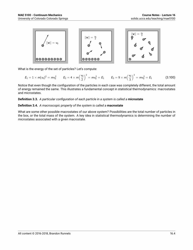
MAE 5100 - Continuum MechanicsUniversity of Colorado Colorado Springs Course Notes - Lecture 16solids.uccs.edu/teaching/mae5100
||v|| = v0
||v|| = v0
2
||v|| = v0
3
What is the energy of the set of particles? Let’s compute:E1 = 1×m(v0)2 = mv2
0 E2 = 4×m(v0
2
)2
= mv20 = E1 E3 = 9×m
(v0
3
)2
= mv20 = E1 (3.100)
Notice that even though the configuration of the particles in each case was completely different, the total amountof energy remained the same. This illustrates a fundamental concept in statistical thermodynamics: macrostatesand microstates.Definition 3.3. A particular configuration of each particle in a system is called a microstate
Definition 3.4. A macroscopic property of the system is called a macrostate
What are some other possible macrostates of our above system? Possibilities are the total number of particles inthe box, or the total mass of the system. A key idea in statistical thermodynamics is determining the number ofmicrostates associated with a given macrostate.
All content © 2016-2018, Brandon Runnels 16.4
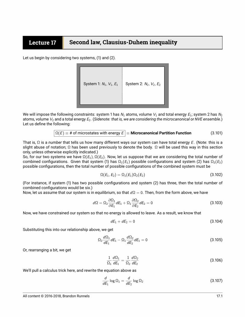
Lecture 17 Second law, Clausius-Duhem inequality
Let us begin by considering two systems, (1) and (2).
System 2: N2,V2,E2System 1: N1,V1,E1
We will impose the following constraints: system 1 has N1 atoms, volume V1 and total energy E1; system 2 has N2atoms, volumeV2 and a total energy E2. (Sidenote: that is, we are considering themicrocanonical or NVE ensemble.)Let us define the following:Ω(E ) ≡ # of microstates with energy E ≡ Microcanonical Partition Function (3.101)
That is, Ω is a number that tells us how many different ways our system can have total energy E . (Note: this is aslight abuse of notation; Ω has been used previously to denote the body. Ω will be used this way in this sectiononly, unless otherwise explicitly indicated.)So, for our two systems we have Ω(E1), Ω(E2). Now, let us suppose that we are considering the total number ofcombined configurations. Given that system (1) has Ω1(E1) possible configurations and system (2) has Ω2(E2)possible configurations, then the total number of possible configurations of the combined system must beΩ(E1,E2) = Ω1(E1)Ω2(E2) (3.102)
(For instance, if system (1) has two possible configurations and system (2) has three, then the total number ofcombined configurations would be six.)Now, let us assume that our system is in equilibrium, so that dΩ = 0. Then, from the form above, we havedΩ = Ω2
∂Ω1
∂E1dE1 + Ω1
∂Ω2
∂E2dE2 = 0 (3.103)
Now, we have constrained our system so that no energy is allowed to leave. As a result, we know thatdE1 + dE2 = 0 (3.104)
Substituting this into our relationship above, we getΩ2
dΩ1
dE1dE1 − Ω1
dΩ2
dE2dE1 = 0 (3.105)
Or, rearranging a bit, we get1
Ω1
dΩ1
dE1=
1
Ω2
dΩ2
dE2(3.106)
We’ll pull a calculus trick here, and rewrite the equation above asd
dE1log Ω1 =
d
dE2log Ω2 (3.107)
All content © 2016-2018, Brandon Runnels 17.1
MAE 5100 - Continuum MechanicsUniversity of Colorado Colorado Springs Course Notes - Lecture 17solids.uccs.edu/teaching/mae5100
Let us define β to beβ1 =
d
dE1log Ω1 β2 =
d
dE2log Ω2 (3.108)
(Again, we restrict our overloading of the termβ to this section only.) This allows us towrite our equilibriumequationas β1 = β2. Now, we notice from the definition thatβdE = d log Ω or dE =
1
βd log Ω (3.109)
Recall that both of our systems have fixed volume and a fixed number of atoms. As a result, we know that the firstlaw of thermodynamics is given by dE = dQ ; in other words, all changes in internal energy must be the result ofheat transfer. We also know that dQ = TdS . This means we can write1
βd log Ω = TdS (3.110)
Here, we identify that 1β ∼ T and d log Ω ∼ dS . In fact, for classical reasons, a constant kB (Boltzmann’s constant)is introduced, giving us
β =1
kBT≡ Reciprocal Temperature S = kB log Ω ≡ Entropy (3.111)
where β is the statistical thermodynamical temperature and S is the total Gibbs entropy of the system. There aresome important notes to be made here:(1) If S1 = kB log Ω1 and S2 = kB log Ω2, then the combined entropy is S = kB log(Ω1Ω2) = kB log Ω1 + kB log Ω2 =
S1 + S2, verifying that entropy is an extensive property of the system.(2) Entropy is interpreted as the number of possiblemicrostates for our system tomaintain its currentmacrostate.This is consistent with the interpretation of entropy as being a “measure of disorder.” For instance, if a coffeecup has fewer possible “microstates” if its macrostate is “being all in one piece” than if its macrostate is“shattered in pieces on the floor.”
If you don’t feel comfortable with the things discussed in this section, that’s ok. The purpose of this section is justto hint at where entropy comes from, in the hope that it will help provide a little bit of intuition. At this point, we willswitch back to continuum mode, where we will work with entropy in a continuum setting.3.5.2 Internal entropy generation
In the previous section we concluded thatdS =
dQ
Tor S =
Q
T(3.112)
In other words, this shows that the rate of increase of entropy is correlated to the rate of heat flowing into thesystem. This is true when the process happens quasistatically and all entropy change in the system is due toexternal contributions. In this case, we say that the process is reversible, because we can return to the originalentropy state by simply removing the previously added heat.For irreversible processes, we allow for the possibility of the system to generate entropy on its own. Thus, we saythat we haveS︸︷︷︸
total entropy change= S int︸︷︷︸
internal entropy generation+
Q
T︸︷︷︸entropy generated externally
(3.113)
As an example, let us consider an adiabatic system (no heat transfer in or out of the system) divided into tworegions with two seperate temperatures as follows:All content © 2016-2018, Brandon Runnels 17.2
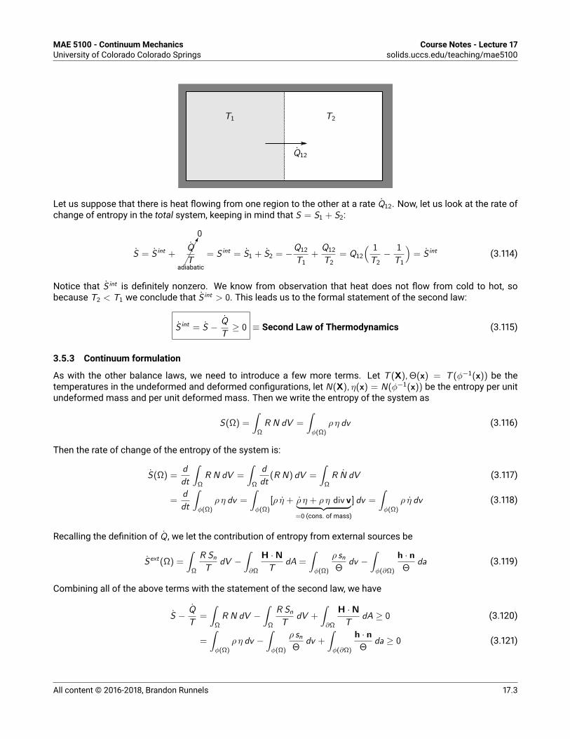
MAE 5100 - Continuum MechanicsUniversity of Colorado Colorado Springs Course Notes - Lecture 17solids.uccs.edu/teaching/mae5100
T1 T2
Q12
Let us suppose that there is heat flowing from one region to the other at a rate Q12. Now, let us look at the rate ofchange of entropy in the total system, keeping in mind that S = S1 + S2:
S = S int +0
Q
Tadiabatic= S int = S1 + S2 = −Q12
T1+
Q12
T2= Q12
( 1
T2− 1
T1
)= S int (3.114)
Notice that S int is definitely nonzero. We know from observation that heat does not flow from cold to hot, sobecause T2 < T1 we conclude that S int > 0. This leads us to the formal statement of the second law:S int = S − Q
T≥ 0 ≡ Second Law of Thermodynamics (3.115)
3.5.3 Continuum formulation
As with the other balance laws, we need to introduce a few more terms. Let T (X), Θ(x) = T (φ−1(x)) be thetemperatures in the undeformed and deformed configurations, let N(X), η(x) = N(φ−1(x)) be the entropy per unitundeformed mass and per unit deformed mass. Then we write the entropy of the system asS(Ω) =
∫Ω
R N dV =
∫φ(Ω)
ρ η dv (3.116)Then the rate of change of the entropy of the system is:
S(Ω) =d
dt
∫Ω
R N dV =
∫Ω
d
dt(R N) dV =
∫Ω
R N dV (3.117)=
d
dt
∫φ(Ω)
ρ η dv =
∫φ(Ω)
[ρ η + ρ η + ρ η div v︸ ︷︷ ︸=0 (cons. of mass)
] dv =
∫φ(Ω)
ρ η dv (3.118)
Recalling the definition of Q , we let the contribution of entropy from external sources beSext(Ω) =
∫Ω
R SnT
dV −∫∂Ω
H ·NT
dA =
∫φ(Ω)
ρ snΘ
dv −∫φ(∂Ω)
h · nΘ
da (3.119)Combining all of the above terms with the statement of the second law, we have
S − Q
T=
∫Ω
R N dV −∫
Ω
R SnT
dV +
∫∂Ω
H ·NT
dA ≥ 0 (3.120)=
∫φ(Ω)
ρ η dv −∫φ(Ω)
ρ snΘ
dv +
∫φ(∂Ω)
h · nΘ
da ≥ 0 (3.121)
All content © 2016-2018, Brandon Runnels 17.3
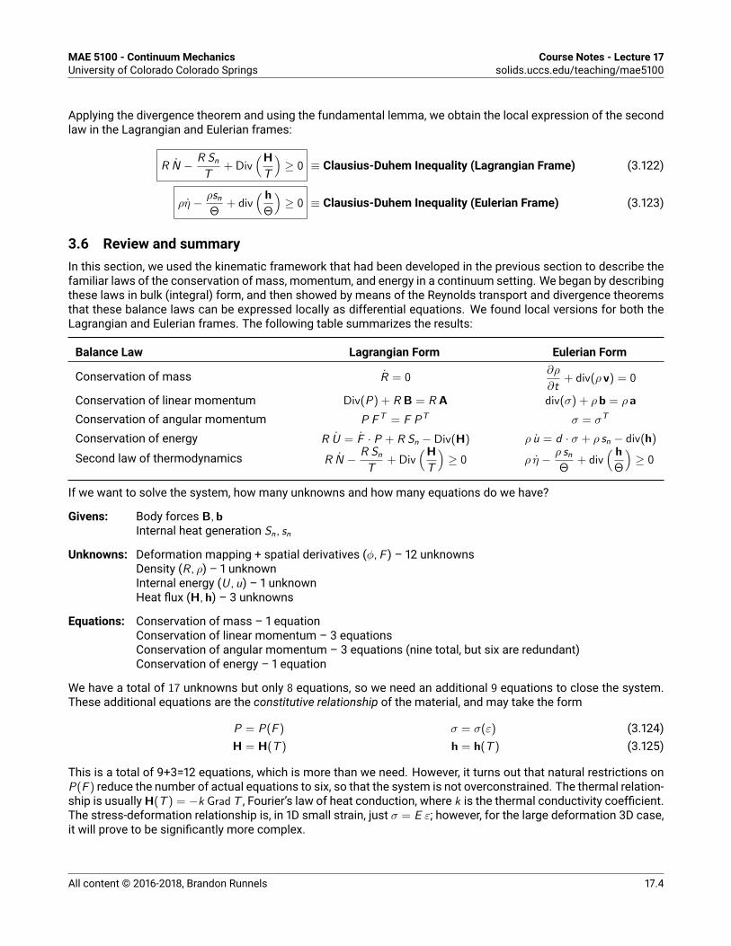
MAE 5100 - Continuum MechanicsUniversity of Colorado Colorado Springs Course Notes - Lecture 17solids.uccs.edu/teaching/mae5100
Applying the divergence theorem and using the fundamental lemma, we obtain the local expression of the secondlaw in the Lagrangian and Eulerian frames:R N − R Sn
T+ Div
(HT
)≥ 0 ≡ Clausius-Duhem Inequality (Lagrangian Frame) (3.122)
ρη − ρsnΘ
+ div( h
Θ
)≥ 0 ≡ Clausius-Duhem Inequality (Eulerian Frame) (3.123)
3.6 Review and summaryIn this section, we used the kinematic framework that had been developed in the previous section to describe thefamiliar laws of the conservation of mass, momentum, and energy in a continuum setting. We began by describingthese laws in bulk (integral) form, and then showed by means of the Reynolds transport and divergence theoremsthat these balance laws can be expressed locally as differential equations. We found local versions for both theLagrangian and Eulerian frames. The following table summarizes the results:Balance Law Lagrangian Form Eulerian Form
Conservation of mass R = 0∂ρ
∂t+ div(ρ v) = 0
Conservation of linear momentum Div(P) + R B = R A div(σ) + ρb = ρ a
Conservation of angular momentum P FT = F PT σ = σT
Conservation of energy R U = F · P + R Sn − Div(H) ρ u = d · σ + ρ sn − div(h)
Second law of thermodynamics R N − R SnT
+ Div(HT
)≥ 0 ρ η − ρ sn
Θ+ div
( h
Θ
)≥ 0
If we want to solve the system, how many unknowns and how many equations do we have?Givens: Body forces B,bInternal heat generation Sn, sn
Unknowns: Deformation mapping + spatial derivatives (φ,F ) – 12 unknownsDensity (R, ρ) – 1 unknownInternal energy (U, u) – 1 unknownHeat flux (H,h) – 3 unknownsEquations: Conservation of mass – 1 equationConservation of linear momentum – 3 equationsConservation of angular momentum – 3 equations (nine total, but six are redundant)Conservation of energy – 1 equationWe have a total of 17 unknowns but only 8 equations, so we need an additional 9 equations to close the system.These additional equations are the constitutive relationship of the material, and may take the form
P = P(F ) σ = σ(ε) (3.124)H = H(T ) h = h(T ) (3.125)
This is a total of 9+3=12 equations, which is more than we need. However, it turns out that natural restrictions onP(F ) reduce the number of actual equations to six, so that the system is not overconstrained. The thermal relation-ship is usuallyH(T ) = −k GradT , Fourier’s law of heat conduction, where k is the thermal conductivity coefficient.The stress-deformation relationship is, in 1D small strain, just σ = E ε; however, for the large deformation 3D case,it will prove to be significantly more complex.
All content © 2016-2018, Brandon Runnels 17.4
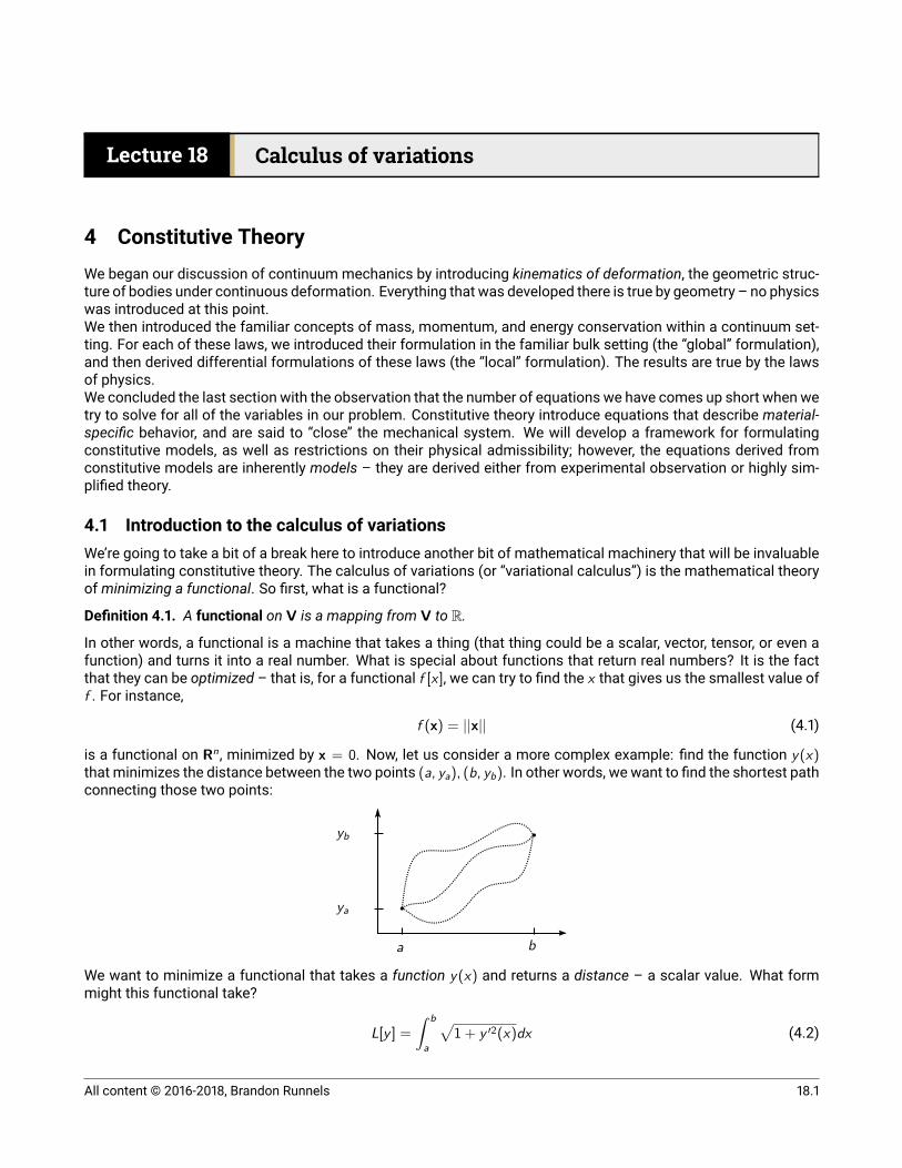
Lecture 18 Calculus of variations
4 Constitutive TheoryWe began our discussion of continuum mechanics by introducing kinematics of deformation, the geometric struc-ture of bodies under continuous deformation. Everything that was developed there is true by geometry – no physicswas introduced at this point.We then introduced the familiar concepts of mass, momentum, and energy conservation within a continuum set-ting. For each of these laws, we introduced their formulation in the familiar bulk setting (the “global” formulation),and then derived differential formulations of these laws (the “local” formulation). The results are true by the lawsof physics.We concluded the last section with the observation that the number of equations we have comes up short when wetry to solve for all of the variables in our problem. Constitutive theory introduce equations that describe material-specific behavior, and are said to “close” the mechanical system. We will develop a framework for formulatingconstitutive models, as well as restrictions on their physical admissibility; however, the equations derived fromconstitutive models are inherently models – they are derived either from experimental observation or highly sim-plified theory.4.1 Introduction to the calculus of variationsWe’re going to take a bit of a break here to introduce another bit of mathematical machinery that will be invaluablein formulating constitutive theory. The calculus of variations (or “variational calculus”) is the mathematical theoryof minimizing a functional. So first, what is a functional?Definition 4.1. A functional on V is a mapping from V to R.
In other words, a functional is a machine that takes a thing (that thing could be a scalar, vector, tensor, or even afunction) and turns it into a real number. What is special about functions that return real numbers? It is the factthat they can be optimized – that is, for a functional f [x ], we can try to find the x that gives us the smallest value off . For instance,
f (x) = ||x|| (4.1)is a functional on Rn , minimized by x = 0. Now, let us consider a more complex example: find the function y(x)that minimizes the distance between the two points (a, ya), (b, yb). In other words, we want to find the shortest pathconnecting those two points:
a b
ya
yb
We want to minimize a functional that takes a function y(x) and returns a distance – a scalar value. What formmight this functional take?L[y ] =
∫ b
a
√1 + y ′2(x)dx (4.2)
All content © 2016-2018, Brandon Runnels 18.1
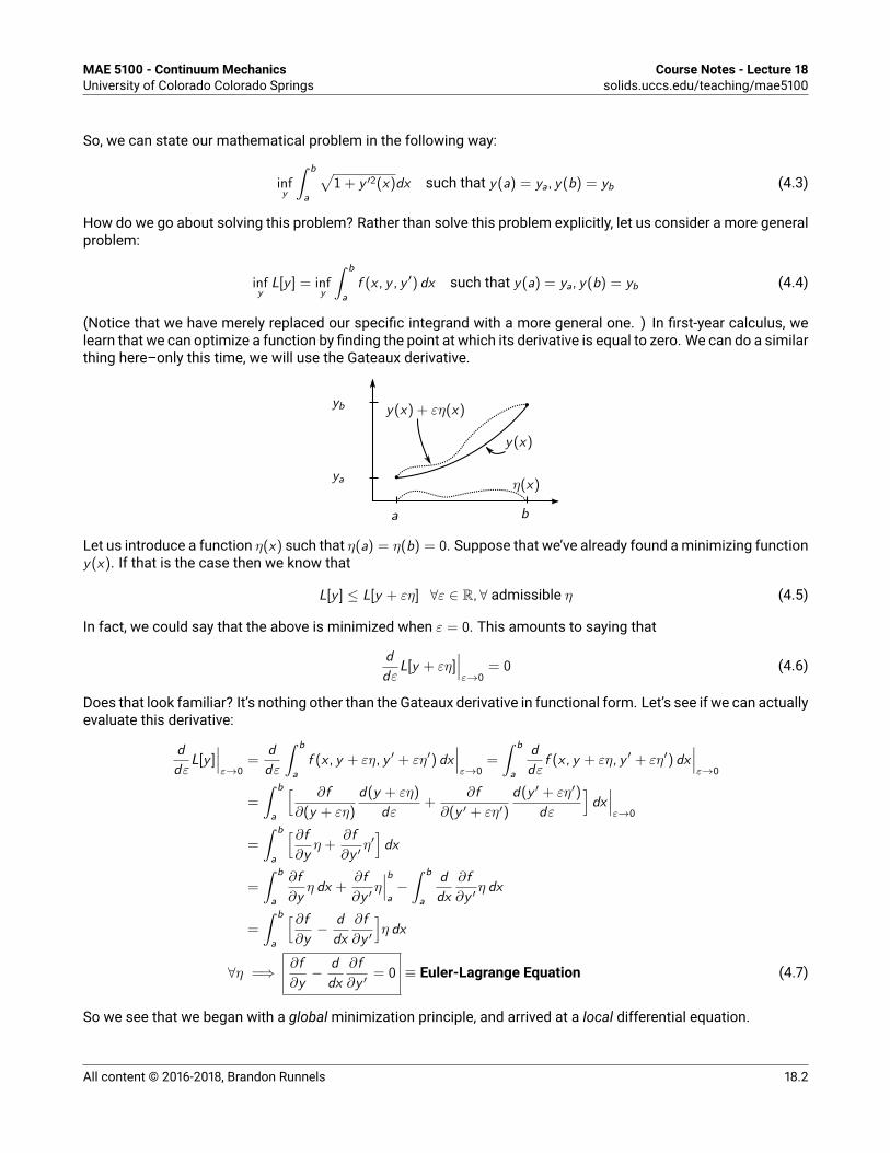
MAE 5100 - Continuum MechanicsUniversity of Colorado Colorado Springs Course Notes - Lecture 18solids.uccs.edu/teaching/mae5100
So, we can state our mathematical problem in the following way:infy
∫ b
a
√1 + y ′2(x)dx such that y(a) = ya, y(b) = yb (4.3)
How do we go about solving this problem? Rather than solve this problem explicitly, let us consider a more generalproblem:infyL[y ] = inf
y
∫ b
a
f (x , y , y ′) dx such that y(a) = ya, y(b) = yb (4.4)(Notice that we have merely replaced our specific integrand with a more general one. ) In first-year calculus, welearn that we can optimize a function by finding the point at which its derivative is equal to zero. We can do a similarthing here–only this time, we will use the Gateaux derivative.
a b
ya
yb
η(x)
y(x)
y(x) + εη(x)
Let us introduce a function η(x) such that η(a) = η(b) = 0. Suppose that we’ve already found aminimizing functiony(x). If that is the case then we know that
L[y ] ≤ L[y + εη] ∀ε ∈ R,∀ admissible η (4.5)In fact, we could say that the above is minimized when ε = 0. This amounts to saying that
d
dεL[y + εη]
∣∣∣ε→0
= 0 (4.6)Does that look familiar? It’s nothing other than the Gateaux derivative in functional form. Let’s see if we can actuallyevaluate this derivative:
d
dεL[y ]
∣∣∣ε→0
=d
dε
∫ b
a
f (x , y + εη, y ′ + εη′) dx∣∣∣ε→0
=
∫ b
a
d
dεf (x , y + εη, y ′ + εη′) dx
∣∣∣ε→0
=
∫ b
a
[ ∂f
∂(y + εη)
d(y + εη)
dε+
∂f
∂(y ′ + εη′)
d(y ′ + εη′)
dε
]dx∣∣∣ε→0
=
∫ b
a
[∂f∂yη +
∂f
∂y ′η′]dx
=
∫ b
a
∂f
∂yη dx +
∂f
∂y ′η∣∣∣ba−∫ b
a
d
dx
∂f
∂y ′η dx
=
∫ b
a
[∂f∂y− d
dx
∂f
∂y ′
]η dx
∀η =⇒ ∂f
∂y− d
dx
∂f
∂y ′= 0 ≡ Euler-Lagrange Equation (4.7)
So we see that we began with a global minimization principle, and arrived at a local differential equation.
All content © 2016-2018, Brandon Runnels 18.2
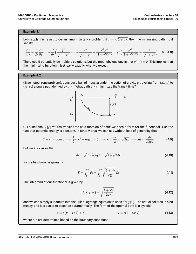
MAE 5100 - Continuum MechanicsUniversity of Colorado Colorado Springs Course Notes - Lecture 18solids.uccs.edu/teaching/mae5100
Example 4.1
Let’s apply this result to our minimum distance problem: if f =√
1 + y ′2, then the minimizing path mustsatisfy∂f
∂y− d
dx
∂f
∂y ′= − d
dx
( y ′√1 + y ′2
)= − y ′′√
1 + y ′2+
y ′2y ′′
(1 + y ′2)3/2= y ′′
( y ′2
(1 + y ′2)3/2− 1√
1 + y ′2
)= 0 (4.8)
There could potentially be multiple solutions, but the most obvious one is that y ′′(x) = 0. This implies thatthe minimizing function y is linear – exactly what we expect.Example 4.2
(Brachistochrone problem): consider a ball of massm under the action of gravity g traveling from (xa, ya) to(xb, yb) along a path defined by y(x). What path y(x) minimizes the transit time?
xa xb
ya
yb
y(x)
Our functional T [y ] returns transit time as a function of path; we need a form for the functional. Use thefact that potential energy is constant, in other words, we can say without loss of generality thatT + U = const =⇒ 1
2mv2 −mg y = 0 =⇒ v =
ds
dt=√
2gy =⇒ dt =ds√2gy
(4.9)But we also know that
ds =√
dx2 + dy2 =√
1 + y ′2dx (4.10)so our functional is given by
T =
∫ tf
ti
dt =
∫ b
a
√1 + y ′2
2gydx (4.11)
The integrand of our functional is given byf (x , y , y ′) =
√1 + y ′2
2gy(4.12)
and we can simply substitute into the Euler Lagrange equation to solve for y(x). The actual solution is a bitmessy, and it is easier to describe parametrically. The form of the optimal path is a cycloid:x = r (θ − sin θ) + c y = r(1− cos θ) (4.13)
where r , c are determined based on the boundary conditions.
All content © 2016-2018, Brandon Runnels 18.3
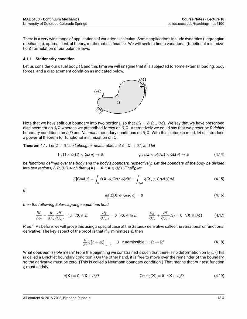
MAE 5100 - Continuum MechanicsUniversity of Colorado Colorado Springs Course Notes - Lecture 18solids.uccs.edu/teaching/mae5100
There is a very wide range of applications of variational calculus. Some applications include dynamics (Lagrangianmechanics), optimal control theory, mathematical finance. We will seek to find a variational (functional minimiza-tion) formulation of our balance laws.4.1.1 Stationarity condition
Let us consider our usual body, Ω, and this time we will imagine that it is subjected to some external loading, bodyforces, and a displacement condition as indicated below.
Ω
∂2Ω
∂1Ω
Note that we have split out boundary into two portions, so that ∂Ω = ∂1Ω ∪ ∂2Ω. We say that we have prescribeddisplacement on ∂1Ω whereas we prescribed forces on ∂2Ω. Alternatively we could say that we prescribe Dirichletboundary conditions on ∂1Ω and Neumann boundary conditions on ∂2Ω. With this picture in mind, let us introducea powerful theorem for functional minimization on Ω:Theorem 4.1. Let Ω ⊂ Rn be Lebesgue measurable. Let φ : Ω→ Rn , and let
f : Ω× φ(Ω)× GL(n)→ R g : ∂Ω× φ(∂Ω)× GL(n)→ R (4.14)be functions defined over the body and the body’s boundary, respectively. Let the boundary of the body be dividedinto two regions, ∂1Ω, ∂2Ω such that φ(X) = X ∀X ∈ ∂1Ω. Finally, let
L[Gradφ] =
∫Ω
f (X,φ, Gradφ)dV +
∫∂2Ω
g(X,φ, Gradφ)dA (4.15)If
infφL[X,φ, Gradφ] = 0 (4.16)
then the following Euler-Lagrange equations hold:
∂f
∂φi− d
dXJ
∂f
∂φi ,J= 0 ∀X ∈ Ω
∂g
∂φi ,J= 0 ∀X ∈ ∂1Ω
∂g
∂φi+
∂f
∂φi ,JNJ = 0 ∀X ∈ ∂2Ω (4.17)
Proof. As before, wewill prove this using a special case of the Gataeux derivative called the variational or functionalderivative. The key aspect of the proof is that if φminimizes L, thend
dεL[φ+ εη]
∣∣∣ε=0
= 0 ∀ admissible η : Ω→ Rn (4.18)What does admissiblemean? From the beginning we constrained φ such that there is no deformation on ∂1φ. (Thisis called a Dirichlet boundary condition.) On the other hand, it is free to move over the remainder of the boundary,so the derivative must be zero. (This is called a Neumann boundary condition.) That means that our test functionη must satisfy
η(X) = 0 ∀X ∈ ∂1Ω Grad η(X) = 0 ∀X ∈ ∂2Ω (4.19)
All content © 2016-2018, Brandon Runnels 18.4
MAE 5100 - Continuum MechanicsUniversity of Colorado Colorado Springs Course Notes - Lecture 18solids.uccs.edu/teaching/mae5100
This will come in very handy in a moment. Now, let us begin by evaluating the derivative:d
dεL[φ+ εη, Grad(φ+ εη)]
∣∣∣ε=0
=
∫Ω
d
dεf (X,φ+ εη, Gradφ+ εGrad η)dV |ε=0+
+
∫∂Ω
d
dεg(X,φ+ εη, Gradφ+ εGrad η)dA
∣∣∣ε=0
=
∫Ω
[ ∂f
∂(φi + εηi )
d(φi + εηi )
dε+
∂f
∂(φi ,J + εηi ,J)
d(φi ,J + εηi ,J)
dε
]dV∣∣∣ε=0
+
∫∂Ω
[ ∂g
∂(φi + εηi )
d(φi + εηi )
dε+
∂g
∂(φi ,J + εηi ,J)
d(φi ,J + εηi ,J)
dε
]dA∣∣∣ε=0
=
∫Ω
[ ∂f∂φi
ηi +∂f
∂φi ,Jηi ,J
]dV +
∫∂Ω
[ ∂g∂φi
ηi +∂g
ηi ,Jηi ,J
]dA (4.20)
Consider the third term. Using the product rule and integration by parts:∫Ω
∂f
∂φi ,Jηi ,JdV =
∫Ω
∂
∂XJ
( ∂f
∂φi ,Jηi
)dV −
∫Ω
d
dXJ
( ∂f
∂φi ,J
)ηidV =
∫∂Ω
∂f
∂φi ,JηiNJdA−
∫Ω
d
dXJ
( ∂f
∂φi ,J
)ηidV
Substituting back into the above expression and gathering terms, we have=
∫Ω
[ ∂f∂φi− d
dXJ
( ∂f
∂φi ,J
)]ηidV +
∫∂Ω
[ ∂g∂φi
ηi +∂g
ηi ,Jηi ,J +
∂f
∂φi ,JηiNJ
]dA (4.21)
Here is where the admissibility condition is useful: let us apply the condition that ηi ,J = 0 everywhere on theboundary except for ∂1Ω. This leaves=
∫Ω
[ ∂f∂φi− d
dXJ
( ∂f
∂φi ,J
)]ηidV +
∫∂1Ω
∂g
ηi ,Jηi ,JdA +
∫∂2Ω
[ ∂g∂φi
+∂f
∂φi ,JNJ
]ηi dA (4.22)
And here is the final payoff: we note that this has to be true for all admissible η. And so, we can pass from the weakform to the strong form by the fundamental lemma. The result is that∂f
∂φi− ∂
∂XJ
∂f
∂φi ,J= 0 ∀X ∈ Ω
∂g
∂φi ,J= 0 ∀X ∈ ∂1Ω
∂g
∂φi+
∂f
∂φi ,JNJ = 0 ∀X ∈ ∂2Ω (4.23)
This concludes the proof.As you can see, the proof of the above theorem is a little bit technical, but it’s really nothing more than a fully 3Dversion of the simple 1D Euler-Lagrange equation that we found earlier. Notice that we left the proof as general aspossible, yet the results are still quite simple. We can now take what we found and apply it directly to continuummechanics.
All content © 2016-2018, Brandon Runnels 18.5
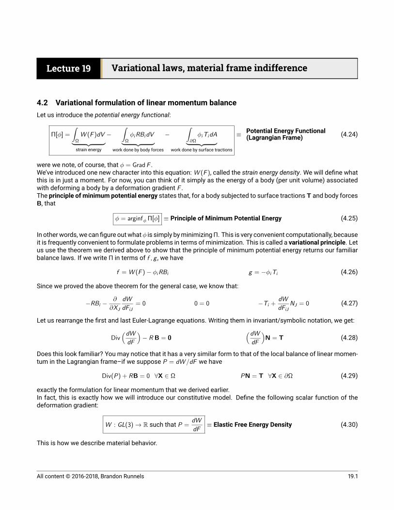
Lecture 19 Variational laws, material frame indifference
4.2 Variational formulation of linear momentum balanceLet us introduce the potential energy functional:
Π[φ] =
∫Ω
W (F )dV︸ ︷︷ ︸strain energy
−∫
Ω
φiRBidV︸ ︷︷ ︸work done by body forces
−∫∂Ω
φiTidA︸ ︷︷ ︸work done by surface tractions
≡ Potential Energy Functional(Lagrangian Frame) (4.24)
were we note, of course, that φ = GradF .We’ve introduced one new character into this equation: W (F ), called the strain energy density. We will define whatthis is in just a moment. For now, you can think of it simply as the energy of a body (per unit volume) associatedwith deforming a body by a deformation gradient F .The principle of minimum potential energy states that, for a body subjected to surface tractionsT and body forcesB, that
φ = arginfφ Π[φ] ≡ Principle of Minimum Potential Energy (4.25)In otherwords, we can figure outwhatφ is simply byminimizingΠ. This is very convenient computationally, becauseit is frequently convenient to formulate problems in terms ofminimization. This is called a variational principle. Letus use the theorem we derived above to show that the principle of minimum potential energy returns our familiarbalance laws. If we write Π in terms of f , g , we have
f = W (F )− φiRBi g = −φiTi (4.26)Since we proved the above theorem for the general case, we know that:
−RBi −∂
∂XJ
dW
dFiJ= 0 0 = 0 −Ti +
dW
dFiJNJ = 0 (4.27)
Let us rearrange the first and last Euler-Lagrange equations. Writing them in invariant/symbolic notation, we get:Div
(dWdF
)− R B = 0
(dWdF
)N = T (4.28)
Does this look familiar? You may notice that it has a very similar form to that of the local balance of linear momen-tum in the Lagrangian frame–if we suppose P = dW /dF we haveDiv(P) + RB = 0 ∀X ∈ Ω PN = T ∀X ∈ ∂Ω (4.29)
exactly the formulation for linear momentum that we derived earlier.In fact, this is exactly how we will introduce our constitutive model. Define the following scalar function of thedeformation gradient:W : GL(3)→ R such that P =
dW
dF≡ Elastic Free Energy Density (4.30)
This is how we describe material behavior.
All content © 2016-2018, Brandon Runnels 19.1
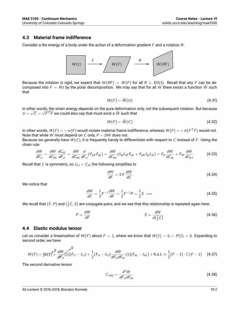
MAE 5100 - Continuum MechanicsUniversity of Colorado Colorado Springs Course Notes - Lecture 19solids.uccs.edu/teaching/mae5100
4.3 Material frame indifferenceConsider a the energy of a body under the action of a deformation gradient F and a rotation R :
F RW (I) W (F ) W (RF )
Because the rotation is rigid, we expect that W (RF ) = W (F ) for all R ∈ SO(3). Recall that any F can be de-composed into F = RU by the polar decomposition. We may say that for all W there exists a function W suchthatW (F ) = W (U) (4.31)
In other words, the strain energy depends on the pure deformation only, not the subsequent rotation. But becauseU =
√C =
√FTF we could also say that must exist a W such that
W (F ) = W (C ) (4.32)In other words, W (F ) = γ tr(F ) would violate material frame indifference, whereas W (F ) = γ tr(FTF ) would not.Note that while W must depend on C only, P = DW does not.Because we generally have W (C ), it is frequently handy to differentiate with respect to C instead of F . Using thechain rule:
dW
dFiJ=
dW
dCKL
dCkL
dFiJ=
dW
dCKL
d
dFiJ(FpKFpL) =
dW
dCKL(δipδJKFpL + FpKδipδJL) = FiL
dW
dCJL+ FiK
dW
dCKJ(4.33)
Recall that C is symmetric, so CIJ = CJI ; the following simplifies todW
dF= 2F
dW
dC(4.34)
We notice thatdW
dC=
1
2F−1 dW
dF=
1
2F−1P =
1
2S =⇒ (4.35)
We recall that (F ,P) and ( 12 C ,S) are conjugate pairs, and we see that this relationship is repeated again here:
P =dW
dFS =
dW
d( 12C )
(4.36)
4.4 Elastic modulus tensorLet us consider a linearization of W (F ) about F = I, where we know that W (I) = 0, = P(I) = 0. Expanding tosecond order, we have
W (F ) =*0
W (I) +>
0dW
dFiJ(I)(FiJ − δiJ) +
1
2(FiJ − δiJ)
dW
dFiJdFkL(I)(FkL − δkL) + h.o.t. ≈ 1
2(F − I) · C (F − I) (4.37)
The second derivative tensorCiJkL =
d2W
dFiJdFkL(4.38)
All content © 2016-2018, Brandon Runnels 19.2
MAE 5100 - Continuum MechanicsUniversity of Colorado Colorado Springs Course Notes - Lecture 19solids.uccs.edu/teaching/mae5100
is called the elastic modulus tensor. It is a useful quantity to compute when solving problems numerically.dW
dFiJ= 2FiI
dW
dC IJ(4.39)
d2W
dFiJdFkL= 2δikδIL
dW
dC IJ+ 2FiI
d
dFkL
dW
dCIJ= 2δik
dW
dCJL+ 2FiI
d2W
dCIJdCKP
dCKP
dFkL= 2δik
dW
dCJL+ 4FiIFkK
d2W
dCIJdCKL(4.40)
= δikdW
d( 12CJL)
+ FiIFkKd2W
d( 12CIJ)d( 1
2CKL)(4.41)
= δikSJL + FiIFkKCIJKL (4.42)We see that CIJKL has both “major symmetry” (CIJKL = CKLIJ ) and “minor symmetry” (CIJKL = CJIKL = CIJLK )4.5 Elastic material modelsWe see from the above that the only thing necessary to define a material model is the free energy function W (F )– given a W , it is always possible to derive P and C. We will illustrate this with a couple of examples.4.5.1 Useful identities
We will be doing a great deal of matrix differentiation, and we frequently have to evaluate complex expressions.The following identities will prove useful:• Derivative of the determinant
d(detF )
dFiJ= det(F )F−TiJ (4.43)
• Derivative of the matrix inversed
dFkLδJM =
d
dFkL(F−1
Jn FnM) =dF−1
Jn
dFkLFnM + F−1
Jn δknδLM =dF−1
Jn
dFkLFnM + F−1
Jk δLM!
= 0 (4.44)dF−1
Jn
dFkLFnMF−1
Mi︸ ︷︷ ︸δni
= −F−1Jk δLMF−1
Mi (4.45)
dF−1Ji
dFkL= −F−1
Jk F−1Li = −F−TkJ F−TiL (4.46)
4.5.2 Pseudo-Linear
A simplistic model that guarantees material frame indifference is the following, where C is a rank-4 tensor andobeys major symmetry (CIJKL = CKLIJ ) and minor symmetry (CIJKL = CJIKL = CIJLK = CJILK ).W (F ) =
1
2E · CE =
1
8(FTF − I) · C (FTF − I) =
1
8(FT
PmFmQ − δPQ)CPQRS (FTRnFnS − δRS) (4.47)
From this definition, we compute the Piola-Kirchoff stress tensor by differentiationDW (F )iJ =
dW
dFiJ=
d
dCAB
[1
8(C − I)C (C − I)
]dCAB
dFiJ=
1
4CABRS (FT
RnFnS − δRS)d
dFiJ(FT
A`F`B)
=1
4CABRS (FT
RnFnS − δRS)(δi`δJAF`B + F`Aδi`δJB)
=1
4(FiBCJBRS + FiACAJRS) (FT
RnFnS − δRS) (4.48)
All content © 2016-2018, Brandon Runnels 19.3
MAE 5100 - Continuum MechanicsUniversity of Colorado Colorado Springs Course Notes - Lecture 19solids.uccs.edu/teaching/mae5100
We compute the elasticity tensor by differentiating againDDW (F )iJkL =
d2W
dFiJdFkL=
d2
dCABdCCD
[1
8(C − I)C (C − I)
]dCAB
dFiJ
dCCD
dFkL+
W
dCAB
[1
8(C − I)C (C − I)
] d2CAB
dFiJdFkL
=1
4(CJALD + CJADL + CAJLD + CAJDL)FiAFkD +
δik4
(CJLRS + CLJRS)FnRFnS −δik4
(CJLRR + CLJRR)
(4.49)The result is somewhat unwieldy, so let us apply symmetry conditions on C to simplify. The result is
DDW (F )iJkL =CAJDL FiAFkD +1
2δik (CLJRS FnRFnS − CJLRR) (4.50)
As a sanity check, we can verify that the stress at F = I must be equal to zero. Substituting, we getP(I)iJ = (δiBCJBRS + δiACAJRS)
:0(δRnδnS − δRS) = 0 X (4.51)
as expected. What happens if we substitute the identity for the elasticity tensor? We obtain:C(I)iJkL =CAJDL δiAδkD +
1
2δik (CLJRS δnRδnS − CJLRR)
=CiJkL +1
2δik (
:0
CLJnn − CJLRR) = CiJkL (4.52)whence we see that the elastic constants correspond to the tangent modulus in the undeformed state.4.5.3 Compressible neo-Hookean
The neo-Hookean model is a simple model that does a fairly good job of modeling rubbery materials. Twomaterialconstants are used, the shear modulus µ and the bulk modulus κ. We define the material by its free energy W (F ):W (F ) =
µ
2
( tr(FTF )
det(F )2/3− 3)
+κ
2(det(F )− 1)2 =
µ
2
( FpQFpQ
det(F )2/3− 3)
+κ
2(det(F )− 1)2 (4.53)
We find the Piola Kirchoff stress tensor which is given by the first derivativeDW (F )iJ =
dW
dFiJ=µ
2
( (FpQFpQ),iJ
det(F )2/3− 2
3
FpQFpQ
det(F )5/3
d det(F )
dFiJ
)+ κ(det(F )− 1)
d det(F )
dFiJ
=µ( FiJ
det(F )2/3− 1
3
FpQFpQ
det(F )2/3F−TiJ
)+ κ(det(F )− 1) det(F )F−TiJ = PiJ
We find the elastic modulus tensor which is given by the second derivativeDDW (F )iJkL =
d2W
dFiJdFkL=
d
dFkL
[µ( FiJ
det(F )2/3− 1
3
FpQFpQ
det(F )2/3F−TiJ
)+ κ(det(F )− 1) det(F )F−TiJ
]=
µ
det(F )2/3
[δikδJL −
2
3FiJF
−TkL −
2
3F−TiJ FkL +
2
9(FpQFpQ)F−TiJ F−TkL +
1
3(FpQFpQ)F−TiL F−TkJ
]+ κ det(F )
[(2 det(F )− 1
)F−TiJ F−TkL +
(1− det(F )
)F−TiL F−TkJ
]= CiJkL (4.54)
Substituting F = I shows quickly that the stress is zero in that state. Substituting into the tangent modulus, wegetDDW (I) =µ (δikδJL + δiLδkJ) +
κ
3δiJδkL (4.55)
where we see that µ and κ correspond to the shear and bulk moduli in small deformation.All content © 2016-2018, Brandon Runnels 19.4
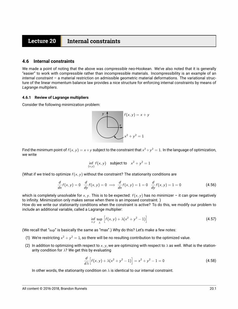
Lecture 20 Internal constraints
4.6 Internal constraintsWe made a point of noting that the above was compressible neo-Hookean. We’ve also noted that it is generally“easier” to work with compressible rather than incompressible materials. Incompressibility is an example of aninternal constraint – a material restriction on admissible geometric material deformations. The variational struc-ture of the linear momentum balance law provides a nice structure for enforcing internal constraints by means ofLagrange multipliers.4.6.1 Review of Lagrange multipliers
Consider the following minimization problem:
x
y f (x , y) = x + y
x2 + y2 = 1
Find theminimum point of f (x , y) = x+y subject to the constraint that x2 +y2 = 1. In the language of optimization,we writeinf
(x ,y)f (x , y) subject to x2 + y2 = 1
(What if we tried to optimize f (x , y) without the constraint? The stationarity conditions ared
dxf (x , y) = 0
d
dyf (x , y) = 0 =⇒ d
dxf (x , y) = 1 = 0
d
dyf (x , y) = 1 = 0 (4.56)
which is completely unsolvable for x , y . This is to be expected: f (x , y) has no minimizer – it can grow negativelyto infinity. Minimization only makes sense when there is an imposed constraint. )How do we write our stationarity conditions when the constraint is active? To do this, we modify our problem toinclude an additional variable, called a Lagrange multiplier:infx ,y
supλ
[f (x , y) + λ(x2 + y2 − 1)
] (4.57)(We recall that “sup” is basically the same as “max”.) Why do this? Let’s make a few notes:(1) We’re restricting x2 + y2 = 1, so there will be no resulting contribution to the optimized value.(2) In addition to optimizing with respect to x , y , we are optimizing with respect to λ as well. What is the station-arity condition for λ? We get this by evaluating
d
dλ
[f (x , y) + λ(x2 + y2 − 1)
]= x2 + y2 − 1 = 0 (4.58)
In other words, the stationarity condition on λ is identical to our internal constraint.
All content © 2016-2018, Brandon Runnels 20.1
MAE 5100 - Continuum MechanicsUniversity of Colorado Colorado Springs Course Notes - Lecture 20solids.uccs.edu/teaching/mae5100
(3) Why are we maximizing with respect to λ? Let’s look at the inside part:supλ
[f (x , y) + λ(x2 + y2 − 1)
]=
0 x2 + y2 = 1
∞ else (4.59)In other words, this inside part will blow up to infinity except if x2 + y2 = 1. Recall that on the outside, we areminimizing with respect to x , y – this means that all non-infinite solutions must satisfy the constraint.
With these notes in mind, let’s attempt to solve the above optimization problem. We have three stationarity condi-tions, which we’ll use to solve for x , y ,λ
dΦ
dx= 1 + 2λx = 0
dΦ
dy= 1 + 2λy = 0
dΦ
dλ= x2 + y2 − 1 = 0 (4.60)
=⇒ x = − 1
2λ=⇒ y = − 1
2λ=⇒ 1
4λ2+
1
4λ2=
1
2λ2= 1 =⇒ λ = ± 1√
2(4.61)
Substituting back, we get two solutions:x = ± 1√
2y = ± 1√
2(4.62)
corresponding to the two points along the x = y line passing through the circle. Exactly what we expect!4.6.2 Examples of internal constraints
Let us express internal constraints for materials such thatψ(F ) = 0 (4.63)
Two examples:• Incompressibility: ψ(F ) = det(F )− 1 = 0
• Inextensible fibers: ψ(F ) = λ2(N)− 1 = NTFTF N− 1 = 0
(Notice that we can write the above constraints entirely in terms of C as well.)4.6.3 Lagrange multipliers in the variational formulation of balance laws
Recall that the equilibrium configuration is given byφ = arg inf
φΠ[φ] = arg inf
φ
[ ∫Ω
W (F )dV −∫
Ω
φiRBidV −∫∂Ω
φiTidA] (4.64)
Let us suppose that we are working with a system that has an internal constraint ψ(F ) = 0. How would we includethis in our optimization problem? Let’s try:arg inf
φsupλ
[Π[φ] +
∫Ω
λφ(F ) dV]
= arg infφ
supλ
[ ∫Ω
(W (F ) + λψ(F )
)dV −
∫Ω
φiRBidV −∫∂Ω
φiTidA] (4.65)
What are our stationarity conditions? For φ, they are nothing other than our usual Euler-Lagrange equations, whichcome out to bedW
dF+ λ
dψ
dF+ RB = 0
(dWdF
+ λdψ
dF
)N = T (4.66)
All content © 2016-2018, Brandon Runnels 20.2
MAE 5100 - Continuum MechanicsUniversity of Colorado Colorado Springs Course Notes - Lecture 20solids.uccs.edu/teaching/mae5100
This prompts us to define the stress tensor to beP =
dW
dF+ λ
dψ
dF(4.67)
Let us look at a couple of examples: first, consider an incompressible material with free energy density W0. Thenψ(F ) = det(F )− 1, and the stress is given by
P =dW
dF+ λ
d
dF(det(F )− 1) = P0 + λ J F−T (4.68)
(where P0 is the stress with the incompressibility constraint removed.) What does this look like in the deformedconfiguration? Apply the relationship between σ and P to obtainσ =
1
JPFT =
1
JP0F
T +1
Jλ J F−TFT = σ0 + λ I (4.69)
In other words, our result is a combination of the regular stress σ0 pluss a “hydrostatic” stress λ I with magnitudeλ. This kind of stress state is identical to hydrostatic pressure, and we generally rename λ to p. Let’s interpret thisresult by noting a couple of points:(1) The material resists all volumetric compression; the way it resists compression is by exerting hydrostaticpressure. Thuswe can interpret Lagrangemultipliers as forces exerted by thematerial to enforce thematerialrestraint.(2) What are the units of p? Recall that λψ(F ) must have units of energy per unit volume, and that ψ(F ) =
det(F )− 1 is unitless. Pressure has units of [force]/[area] which can be written as [force][length]/[volume].
All content © 2016-2018, Brandon Runnels 20.3
Lecture 21 Linearized constitutive theory & Coleman-Noll
4.7 Linearized constitutive theoryAt the end of the section on kinematics, we introduced a framework for linearized kinematics, in which we replacethe deformation mapping φ with the displacement field u, powers and gradients of order greater than two aresufficiently small to ignore.Let us assume that we can express the energy of our material under small strain as W (ε). Then the principal ofminimum potential energy becomes
u = arg infu
[ ∫Ω
W (ε)dV −∫
Ω
u · b dV −∫∂Ω
u · tdS] (4.70)
The Euler-Lagrange for this problem (in the static case) givediv(dWdε
)+ ρb = 0 (4.71)
We compare this with the local balance of linear momentum, which is given bydiv(σ) + ρb = ρu (4.72)
(note that u = a.) This implies that the Cauchy stress is given byσ =
dW
dεσij =
dW
dεij(4.73)
What form must W (ε) take? Let us Taylor expand about ε = 0:W (ε) = W (0) +
dW
dεij(0) εij +
1
2
d2W
dεijdεkl(0) εij εkl + h.o.t. (4.74)
We can statewithout loss of generality thatW (0); also, we assume that ourmaterial is purely elastic, soDW (0) = 0.Thus we are left withW (ε) =
1
2
d2W
dεijdεklεij εkl =
1
2Cijkl εij εkl (4.75)
where Cijkl is a fourth order tensor containing the constant elastic moduli of the material. This is amenable todifferentiation, so that our stress tensor is given byσij =
dW
dεij= Cijklεkl (4.76)
Finally, we write our momentum balance equation in the following way:Cijklεkl ,j + ρbi = ρui (4.77)
4.7.1 Major & minor symmetry and Voigt notation
We have established that in small strain, the elastic modulus tensor is defined byCijkl =
d2W
dεijdεkl(4.78)
This is an order 3× 3× 3× 3 tensor, meaning that it can contain up to 34 = 81 elastic constants – far too many tokeep track of easily. Indeed, the above is too general: we can use symmetry arguments to reduce the number ofpossible constants:All content © 2016-2018, Brandon Runnels 21.1
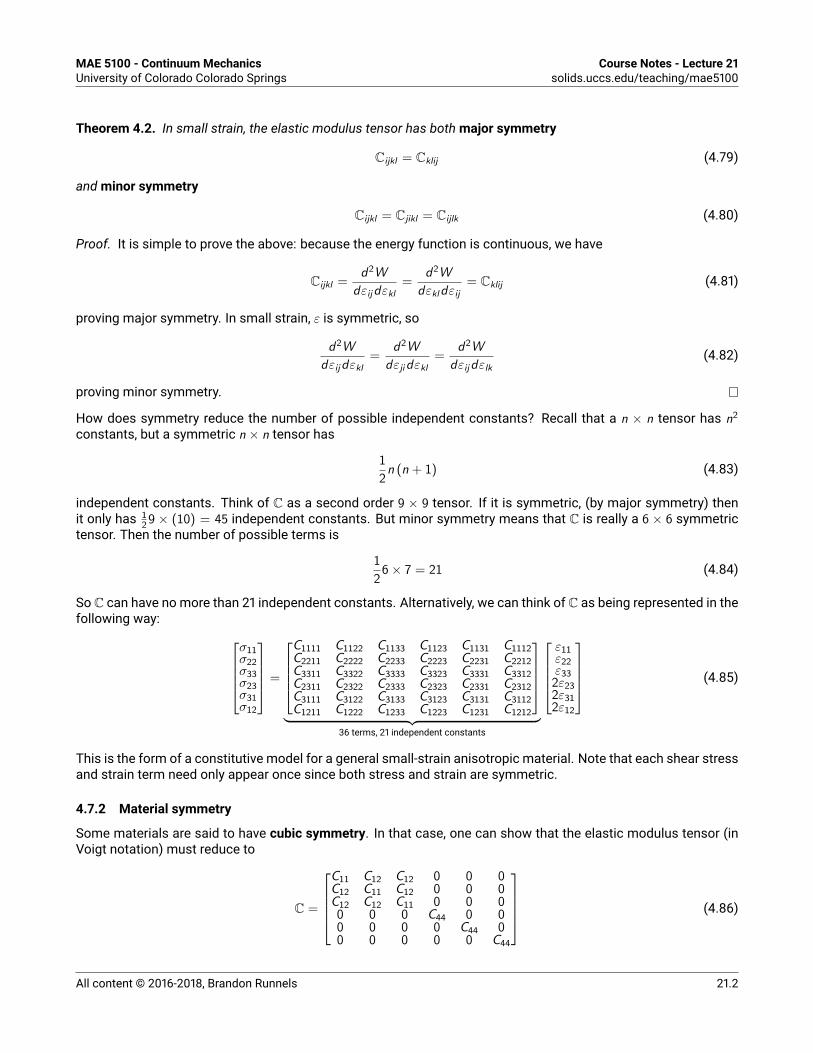
MAE 5100 - Continuum MechanicsUniversity of Colorado Colorado Springs Course Notes - Lecture 21solids.uccs.edu/teaching/mae5100
Theorem 4.2. In small strain, the elastic modulus tensor has both major symmetry
Cijkl = Cklij (4.79)and minor symmetry
Cijkl = Cjikl = Cijlk (4.80)Proof. It is simple to prove the above: because the energy function is continuous, we have
Cijkl =d2W
dεijdεkl=
d2W
dεkldεij= Cklij (4.81)
proving major symmetry. In small strain, ε is symmetric, sod2W
dεijdεkl=
d2W
dεjidεkl=
d2W
dεijdεlk(4.82)
proving minor symmetry.How does symmetry reduce the number of possible independent constants? Recall that a n × n tensor has n2
constants, but a symmetric n × n tensor has1
2n (n + 1) (4.83)
independent constants. Think of C as a second order 9 × 9 tensor. If it is symmetric, (by major symmetry) thenit only has 12 9 × (10) = 45 independent constants. But minor symmetry means that C is really a 6 × 6 symmetrictensor. Then the number of possible terms is
1
26× 7 = 21 (4.84)
So C can have no more than 21 independent constants. Alternatively, we can think of C as being represented in thefollowing way: σ11σ22σ33σ23σ31σ12
=
C1111 C1122 C1133 C1123 C1131 C1112C2211 C2222 C2233 C2223 C2231 C2212C3311 C3322 C3333 C3323 C3331 C3312C2311 C2322 C2333 C2323 C2331 C2312C3111 C3122 C3133 C3123 C3131 C3112C1211 C1222 C1233 C1223 C1231 C1212
︸ ︷︷ ︸
36 terms, 21 independent constants
ε11ε22ε33
2ε232ε312ε12
(4.85)
This is the form of a constitutive model for a general small-strain anisotropic material. Note that each shear stressand strain term need only appear once since both stress and strain are symmetric.4.7.2 Material symmetry
Some materials are said to have cubic symmetry. In that case, one can show that the elastic modulus tensor (inVoigt notation) must reduce to
C =
C11 C12 C12 0 0 0C12 C11 C12 0 0 0C12 C12 C11 0 0 00 0 0 C44 0 00 0 0 0 C44 00 0 0 0 0 C44
(4.86)
All content © 2016-2018, Brandon Runnels 21.2
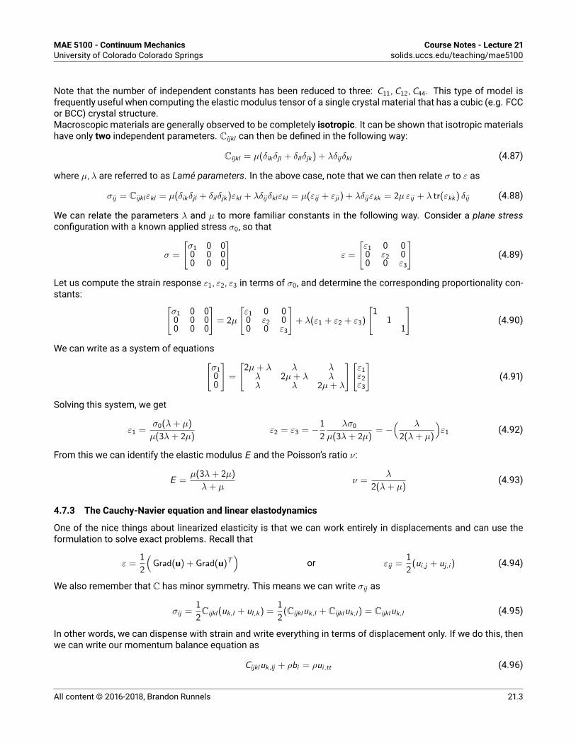
MAE 5100 - Continuum MechanicsUniversity of Colorado Colorado Springs Course Notes - Lecture 21solids.uccs.edu/teaching/mae5100
Note that the number of independent constants has been reduced to three: C11,C12,C44. This type of model isfrequently useful when computing the elastic modulus tensor of a single crystal material that has a cubic (e.g. FCCor BCC) crystal structure.Macroscopic materials are generally observed to be completely isotropic. It can be shown that isotropic materialshave only two independent parameters. Cijkl can then be defined in the following way:Cijkl = µ(δikδjl + δilδjk) + λδijδkl (4.87)
where µ,λ are referred to as Lamé parameters. In the above case, note that we can then relate σ to ε asσij = Cijklεkl = µ(δikδjl + δilδjk)εkl + λδijδklεkl = µ(εij + εji ) + λδijεkk = 2µ εij + λ tr(εkk) δij (4.88)
We can relate the parameters λ and µ to more familiar constants in the following way. Consider a plane stressconfiguration with a known applied stress σ0, so thatσ =
[σ1 0 00 0 00 0 0
]ε =
[ε1 0 00 ε2 00 0 ε3
](4.89)
Let us compute the strain response ε1, ε2, ε3 in terms of σ0, and determine the corresponding proportionality con-stants: [σ1 0 00 0 00 0 0
]= 2µ
[ε1 0 00 ε2 00 0 ε3
]+ λ(ε1 + ε2 + ε3)
[1
11
](4.90)
We can write as a system of equations[σ100
]=
[2µ+ λ λ λλ 2µ+ λ λλ λ 2µ+ λ
][ε1ε2ε3
](4.91)
Solving this system, we getε1 =
σ0(λ+ µ)
µ(3λ+ 2µ)ε2 = ε3 = −1
2
λσ0
µ(3λ+ 2µ)= −
( λ
2(λ+ µ)
)ε1 (4.92)
From this we can identify the elastic modulus E and the Poisson’s ratio ν:E =
µ(3λ+ 2µ)
λ+ µν =
λ
2(λ+ µ)(4.93)
4.7.3 The Cauchy-Navier equation and linear elastodynamics
One of the nice things about linearized elasticity is that we can work entirely in displacements and can use theformulation to solve exact problems. Recall thatε =
1
2
(Grad(u) + Grad(u)T
) or εij =1
2(ui ,j + uj ,i ) (4.94)
We also remember that C has minor symmetry. This means we can write σij asσij =
1
2Cijkl(uk,l + ul ,k) =
1
2(Cijkluk,l + Cijkluk,l) = Cijkluk,l (4.95)
In other words, we can dispense with strain and write everything in terms of displacement only. If we do this, thenwe can write our momentum balance equation asCijkluk,lj + ρbi = ρui ,tt (4.96)
All content © 2016-2018, Brandon Runnels 21.3
MAE 5100 - Continuum MechanicsUniversity of Colorado Colorado Springs Course Notes - Lecture 21solids.uccs.edu/teaching/mae5100
Substituting the form for isotropic elasticityThis is referred to in general as the Cauchy-Navier equation. It is a linear second order PDE in space and time thatcan be solved relatively easily. Let’s consider a 1D plane strain version of the problem. Then we can writeσ = 2µ
[u1,1(t) 0 0
0 0 00 0 0
]+ λ u1,1(t)
[1
11
](4.97)
Thendiv σ =
[(2µ+ λ)u1,11
00
](4.98)
If we ignore body forces, then the Cauchy Navier equation becomes(2µ+ λ)
∂2u
∂x21
= ρ∂2u
∂t2, (4.99)
equation that can be analyzed easily using the method of characteristics or seperation of variables.4.8 Thermodynamics of solids and the Coleman-Noll frameworkWe now return to finite strain mechanics. We have treated the formulation of pure elasticity, which is completelyreversible. However there are multiple types of mechanical phenomena such as plasticity and viscoelasticity thatare irreversible. Additionally, wewish to keep our treatment as general as possible, sowe aim to account for thermaleffects in addition to mechanical.Towards this end, we begin by assuming that a material can locally be defined by(1) The deformation gradient F and its derivatives (although we will only consider F here)(2) The material entropy N (per unit undeformed mass) and its derivatives(3) A set of internal variables that we will denote in vector form by Q. (Note that Q isn’t a vector in the spatialsense, rather it’s just a collection of individual internal variables.) A good example of an internal variable isthe accumulated plastic deformation in a material.
Now, let us assume that there exists an internal energy functional U = U(F ,N,Q) that characterizes the materialsresponse to deformation, entropy, and change in internal variables.Let us begin by working with the Clasius-Duhem inequaltiy: start by expanding it out using the product rule.RN + Div
(HT
)− RSn
T=product rule RN +
1
TDivH− 1
T 2HGradT − RSn
T≥ 0 (4.100)
We spot the appearance of the DivH term: we’ve seen this before in the first law in the Lagrangian frame. Rear-ranging the first law, we can solve for it:RU = P · F + RSn − DivH =⇒ DivH = P · F + RSn − RU (4.101)
Now, we can substitute this into the Clasius-Duhem inequality, and because T > 0 we can multiply out by T :RN +
P · F + RSn − RU
T− 1
T 2HGradT − RSn
T≥ 0 (4.102)
RTN − RU + P · F − 1
THGradT ≥ 0 (4.103)
All content © 2016-2018, Brandon Runnels 21.4
MAE 5100 - Continuum MechanicsUniversity of Colorado Colorado Springs Course Notes - Lecture 21solids.uccs.edu/teaching/mae5100
Now, let’s consider the internal energy functional. Because its a function of F ,N,Q, we can expand its time deriva-tive out using the chain rule:U =
∂U
∂F· F +
∂U
∂NN +
∂U
∂Q· Q (4.104)
Substituting this relationship back into the inequality, we getRTN − R
∂U
∂FF − R
∂U
∂NN − R
∂U
∂Q· Q− P · F − 1
THGradT ≥ 0 (4.105)
And finally, we gather terms:(P − R
∂U
∂F
)︸ ︷︷ ︸ ·F +
(RT − R
∂U
∂N
)︸ ︷︷ ︸ N + R
∂U
∂Q︸ ︷︷ ︸ ·Q−1
THGradT︸ ︷︷ ︸ ≥ 0 (4.106)
The arbitrary nature of F , N, Q prompt us to identify the following definitions:Pe = R
∂U
∂F︸ ︷︷ ︸Elastic stress
Pv = P − Pe︸ ︷︷ ︸Viscous stress
T =∂U
∂N︸ ︷︷ ︸Temperature
Y = −R ∂U∂Q︸ ︷︷ ︸
Dissipative driving force(4.107)
Let’s discuss the new quantities briefly:(1) Pe is the component of the stress that is purely elastic, for instance, the stress computed by Hooke’s law.(2) Pv is the part of the stress corresponding to dissipation, for instance, the viscous stress generated in a fluid.(3) Y is a bit more abstract. Components ofY correspond to components ofQ, and you can think of them as theforces that cause the internal variables to change. For instance, for the internal variable of plastic dissipation,the driving force is the component of the stress that forces the plastic slip.
With these newly defined quantities, we can write the second law of thermodynamics asPv · F︸ ︷︷ ︸
mechanical+ Y · Q︸ ︷︷ ︸
internal− 1
TH · GradT︸ ︷︷ ︸thermal
≥ 0 (4.108)
This implies that irreversible (entropy-generating) processes can take three forms: (i) mechanical dissipation (e.g.viscous drag in fluid flow) (ii) internal dissipation (e.g. plasticity) and (iii) thermal dissipation.
All content © 2016-2018, Brandon Runnels 21.5
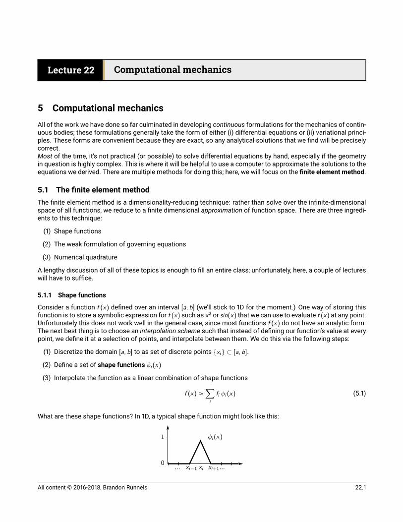
Lecture 22 Computational mechanics
5 Computational mechanicsAll of the work we have done so far culminated in developing continuous formulations for the mechanics of contin-uous bodies; these formulations generally take the form of either (i) differential equations or (ii) variational princi-ples. These forms are convenient because they are exact, so any analytical solutions that we find will be preciselycorrect.Most of the time, it’s not practical (or possible) to solve differential equations by hand, especially if the geometryin question is highly complex. This is where it will be helpful to use a computer to approximate the solutions to theequations we derived. There are multiple methods for doing this; here, we will focus on the finite element method.5.1 The finite element methodThe finite element method is a dimensionality-reducing technique: rather than solve over the infinite-dimensionalspace of all functions, we reduce to a finite dimensional approximation of function space. There are three ingredi-ents to this technique:(1) Shape functions(2) The weak formulation of governing equations(3) Numerical quadrature
A lengthy discussion of all of these topics is enough to fill an entire class; unfortunately, here, a couple of lectureswill have to suffice.5.1.1 Shape functions
Consider a function f (x) defined over an interval [a, b] (we’ll stick to 1D for the moment.) One way of storing thisfunction is to store a symbolic expression for f (x) such as x2 or sin(x) that we can use to evaluate f (x) at any point.Unfortunately this does not work well in the general case, since most functions f (x) do not have an analytic form.The next best thing is to choose an interpolation scheme such that instead of defining our function’s value at everypoint, we define it at a selection of points, and interpolate between them. We do this via the following steps:(1) Discretize the domain [a, b] to as set of discrete points xi ⊂ [a, b].(2) Define a set of shape functions φi (x)
(3) Interpolate the function as a linear combination of shape functionsf (x) ≈
∑i
fi φi (x) (5.1)
What are these shape functions? In 1D, a typical shape function might look like this:φi (x)
xi−1 xi xi+10
1
......
All content © 2016-2018, Brandon Runnels 22.1
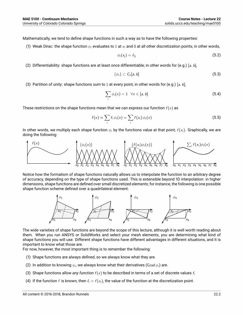
MAE 5100 - Continuum MechanicsUniversity of Colorado Colorado Springs Course Notes - Lecture 22solids.uccs.edu/teaching/mae5100
Mathematically, we tend to define shape functions in such a way as to have the following properties:(1) Weak Dirac: the shape function φi evaluates to 1 at xi and 0 at all other discretization points; in other words,
φi (xj) = δij (5.2)(2) Differentiability: shape functions are at least once differentiable; in other words for (e.g.) [a, b],
φi ⊂ C1[a, b] (5.3)(3) Partition of unity: shape functions sum to 1 at every point; in other words for (e.g.) [a, b],∑
i
φi (x) = 1 ∀x ∈ [a, b] (5.4)
These restrictions on the shape functions mean that we can express our function f (x) asf (x) ≈
∑i
fi φi (x) =∑i
f (xi )φi (x) (5.5)In other words, we multiply each shape function φi by the functions value at that point, f (xi ). Graphically, we aredoing the following:
f (x) φi (x)
x0 x1 x2 x3 x4 x5 x6 x7 x8 x0 x1 x2 x3 x4 x5 x6 x7 x8
f (xi )φi (x)∑
i f (xi )φi (x)
x0 x1 x2 x3 x4 x5 x6 x7 x8
Notice how the formalism of shape functions naturally allows us to interpolate the function to an arbitrary degreeof accuracy, depending on the type of shape functions used. This is extensible beyond 1D interpolation: in higherdimensions, shape functions are defined over small discretized elements; for instance, the following is one possibleshape function scheme defined over a quadrilateral element:
x1 x2
x3 x4
x1 x2
x3 x4
x1 x2
x3 x4
x1 x2
x3 x4
φ1 φ2 φ3 φ4
The wide varieties of shape functions are beyond the scope of this lecture, although it is well worth reading aboutthem. When you run ANSYS or SolidWorks and select your mesh elements, you are determining what kind ofshape functions you will use. Different shape functions have different advantages in different situations, and it isimportant to know what those are.For now, however, the most important thing is to remember the following:(1) Shape functions are always defined, so we always know what they are.(2) In addition to knowing φi , we always know what their derivatives (Gradφi ) are.(3) Shape functions allow any function f (x) to be described in terms of a set of discrete values fi
(4) If the function f is known, then fi = f (xi ), the value of the function at the discretization point.All content © 2016-2018, Brandon Runnels 22.2
MAE 5100 - Continuum MechanicsUniversity of Colorado Colorado Springs Course Notes - Lecture 22solids.uccs.edu/teaching/mae5100
5.1.2 Weak formulation
Consider a domain Ω with a set of discretization points xi ⊂ Ω and shape functions φi ⊂ C1(Ω). (If it is helpful,you can think of Ω = [a, b], the 1D case.)Now, let us suppose that we wish to solve a linear partial differential equation (in space only, no time dependence)that is defined over Ω, with boundary conditions defined on ∂Ω. In 1D, an example might bed2f
dx2+ f (x) = g(x) (5.6)
We can write a differential equation of this form more generally:D[f ]− g(x) = 0 (5.7)
where D[f ] is a generalized way of writing all contains all of the derivatives and scalar multipliers on f , and gcontains “everything else.” Recall that we can write f asf (x) =
∑fi φi (x), (5.8)
so we can express the above asD[∑
i
fiφi (x)]− g(x) =
∑i
fi D[φi (x)]− g(x) = 0 (5.9)Now, recall the fundamental lemma of the Calculus of Variations? It works both ways: if the above is true, then wecan say that ∫
Ω
[∑i
fi D[φi (x)]− g(x)]η(x) dx = 0 ∀η (5.10)
This is called the weak form. Here’s the important step: remember that η can be anything – so why not let it beη(x) =
∑i
ηi φi (x). (5.11)If we make this substitution, we have∫
Ω
[∑i
fi D[φi (x)]− g(x)] (∑
j
ηjφj(x))dx = 0 ∀ηj (5.12)
It may seem that we just took an easy problem and made it complicated. Let’s rearrange it to try to simplify:∑i
∑j
fi ηj
∫Ω
D[φi (x)]φj(x) dx =∑j
ηj
∫Ω
g(x)φj(x) dx ∀ηj (5.13)Now, recall that the above must hold true for every possible value of ηj . The only way for this to be possible is ifthe following is true as well: ∑
i
fi
∫Ω
D[φi (x)]φj(x) dx =
∫Ω
g(x)φj(x) dx (5.14)(This is the equivalent of passing from the weak form to the strong form in the discretized case.) So, what is theadvantage of writing our problem this way? Recall that we are trying to find fi – if we can find them, then wecan construct an interpolated solution to the problem. If we look through the problem, we will see that we already
All content © 2016-2018, Brandon Runnels 22.3
MAE 5100 - Continuum MechanicsUniversity of Colorado Colorado Springs Course Notes - Lecture 22solids.uccs.edu/teaching/mae5100
know everything else: we know φi so we can compute the integral containing D[φi ], and we know g(x) so we cancompute the second integral as well. We might write the problem this way:fi Kij = bj (5.15)
whereKij =
∫Ω
D[φi (x)]φj(x) dx bj =
∫Ω
g(x)φj(x) dx (5.16)K is frequently called the stiffness matrix and b the vector of forces, because the finite element method was his-torically developed for solid mechanics. Remember, we can compute K and b directly, so the resulting problem isa simple linear solve – quite doable by computer!We glossed over some details here, so let’s make a few notes:
• The integralKij =
∫Ω
D[φi (x)]φj(x) dx (5.17)can generally be reduced to a more symmetric form using integration by parts.
• Recall that we let our arbitrary function η be described asη(x) =
∑j
ηj φj(x) (5.18)Actually, this was something of a design decision: the selection of η to that form is a particular choice, and ispart of the so-called Galerkin method. There are other discretization methods, but this is generally the mostpopular.
5.1.3 Numerical quadrature
Numerical quadrature is nothing other than a fancy term for integral approximation. Recall that we casually statedthat the integralKij =
∫Ω
D[φi (x)]φj(x) dx (5.19)was easy to compute, sincewe knowD and φi. It would bemore accurate to say that it is possible to compute – inreality, the integral is not necessarily computable easily, especially if we are working with a geometrically complexmesh.Quadrature is just a method for approximating a nasty integral by evaluating it a specific points. For instance asimple so-called “quadrature rule” for a 1D integral might be written this way:∫
Ω
f (x) dx ≈∑α
qαf (xα) (5.20)where we would call xα quadrature points and qα quadrature weights. For an integral over an element, thereare conveniently tabulated quadrature points and weights that enable accurate and efficient integral evaluation.
All content © 2016-2018, Brandon Runnels 22.4
Lecture 23 FEM and CFD
5.2 Linearized kinematicsLet us consider the equation of conservation of linear momentum for the static case in one dimension, where planestress is assumed:
Ed2u
dx2+ b(x) = 0 (5.21)
Suppose we have a discretization xi and shape functions φi , and our domain is Ω = [a, b] Let us find the finiteelement formulation of this equation. First, letu(x) = ui φi (x) (5.22)
so that the equation can be written as ∑i
ui Ed2φidx2
+ b(x) = 0 (5.23)Now, we can express the above in weak form as∫ b
a
[∑i
ui Ed2φidx2
+ b(x)]η(x) dx = 0 ∀η (5.24)
Applying the Galerkin method, we can write the above as∑i
ui ηJ
∫ b
a
Ed2φidx2
φj(x) dx = −∑j
ηj
∫ b
a
b(x)φj(x) dx ∀ηj (5.25)Passing back to the strong form, we have
∑i
ui
∫ b
a
Ed2φidx2
φj(x) dx︸ ︷︷ ︸Kij
= −∫ b
a
b(x)φj(x) dx (5.26)
We can use integration by parts to reduce the stiffness matrix a little more:Kij =
∫ b
a
Ed2φidx2
φj(x) dx =dφidx2
φj(x)∣∣∣ba︸ ︷︷ ︸
=0
−∫ b
a
E(dφidx
)(dφjdx
)dx (5.27)
Thus, we can write the equilibrium equation as∑j
[∫ b
a
E(dφidx
)(dφjdx
)dx
]uj =
∫ b
a
b(x)φi (x) dx (5.28)We note that this modified version of the stiffness matrix has one huge advantage: it only requires that the shapefunctions be differentiable once, whereas the previous required twice differentiability. It is definitely possible touse “higher order” shape functions that are differentiable this way, but they frequently come with their own set ofdisadvantages.
All content © 2016-2018, Brandon Runnels 23.1
MAE 5100 - Continuum MechanicsUniversity of Colorado Colorado Springs Course Notes - Lecture 23solids.uccs.edu/teaching/mae5100
5.2.1 3D linearized elasticity
Let us now develop the finite element formulation of a fully 3d linear elastic material, for which the equations areCijkluk,lj + ρ bi = ρui (5.29)
Given a domain Ω with discretization xm and shape functions φm ⊂ C1(Ω), we begin by discretizing our dis-placement field:ui (x) = umi φ
m(x) (5.30)(Note that we (i) adopt the summation convention, and (ii) use superscripts to indicate summation over all shapefunctions, as opposed to subscripts summing over all dimensions.) Substituting into our governing equation, wehave
umk Cijkl φm,lj + ρ bi = ρumi φ
m (5.31)Again, we write in weak form ∫
Ω
[umk Cijkl φm,lj + ρ bi − ρumi φm] ηi (x) dv = 0 ∀η(x) (5.32)
(Notice that we are dotting with η.) Adopting a Galerkin discretization (ηi = ηni φn), we can now write
umk ηni
∫Ω
Cijkl φm,ljφ
n dv + ηni
∫Ω
ρ biφn dv = umi η
ni
∫Ω
ρ φm φn dv ∀ηni (5.33)Because this holds for all test functions, we have
umk
∫Ω
Cijkl φm,ljφ
n dv +
∫Ω
ρ biφn dv = umi
∫Ω
ρ φm φn dv (5.34)Applying the product rule and rearranging,
umk
∫Ω
Cijkl φm,j φ
n,l dv + umi
∫Ω
ρ φm φn dv =
∫Ω
ρ biφn dv (5.35)
For the static case, we have a simple linear system to solve. For the dynamic case (with no body forces) we have alinear eigenvalue problem, where the eigenvalues of the stiffness matrix correspond to resonant frequencies, andthe eigenvectors to resonant modes.5.3 Newton’s methodNewton’s method is a powerful technique for solving many kinds of variational problems. Suppose that we have afunction f (x) that we wish to optimize, and suppose we have an initial guess x0. Let us expand f (x) about x0:
f (x) ≈ f (x0) + f ′(x0)(x − x0) +1
2f ′′(x0)(x − x0)2 (5.36)
What is the optimal point of the above approximated function?df
dx= f ′(x0) + f ′′(x0)(x − x0)
!= 0 =⇒ x = x0 −
f ′(x0)
f ′′(x0)(5.37)
Does this equation give us the exact solution? It depends: if it happens that f (x) was quadratic, then yes. Otherwise,we don’t really know – although it is a good bet that the new point x got us much closer to the actual solution.All content © 2016-2018, Brandon Runnels 23.2
MAE 5100 - Continuum MechanicsUniversity of Colorado Colorado Springs Course Notes - Lecture 23solids.uccs.edu/teaching/mae5100
What about if we have F (x), a vector functional? We can do exactly the same thing: if our initial guess is xn thenF (x) ≈ F (xn) + DF (xn)p(xp − xnp ) +
1
2DDF (xn)pq(xp − xnp )(xq − xnq ) (5.38)
Using the stationarity condition we getdF
dxi= DF (xn)i + DDF (xn)ij(xj − xnj )
!= 0 (5.39)
Solving for x givesxj = xnj − DDF (xn)−1
ji DF (xn)i (5.40)The Newton iteration is then defined to be
xn+1 = xn − DDF (xn)−1DF (xn) (5.41)5.4 Finite kinematicsWe introduce the following discretization:
φ(X) ≈∑α
φαηα(X) =summation convention φαηα(X) (5.42)
where φ are vector-valued constants and ηα(X) are shape functions that are at least C 0 continuous (so thegradient can be computed). We recall the variational statement of theφ = arg inf
φΠ[φ] = arg inf
φ
[∫Ω
W (F )dV −∫
Ω
φiRBidV −∫∂Ω
φiTidA
](5.43)
Our finite element scheme admits the statement of the following discretized problem:φ = arg inf
φΠ[φ] = arg inf
φ
∫Ω
W (φκ Grad ηκ)dV −∫
Ω
φκi ηκRBidV −
∫∂Ω
φκi ηκTidA (5.44)
The variational structure of the problem enables a ready solution by means of Newton’s method. Beginning withan initial guess φ0, the following iteration converges to the solution:φαi 7→ φαi − (DDΠ−1)αβij DΠβj (5.45)
where we computeΠ[φ] =
∫Ω
W (φκ Grad ηκ)dV −∫
Ω
φκi ηκRBidV −
∫∂Ω
φκi ηκTidA (5.46)
DΠ[φ]αi =dΠ
dφαi=
∫Ω
DW (φκ Grad ηκ)ip Grad ηα,p dV −∫
Ω
ηαRBidV −∫∂Ω
ηαTidA = 0 (5.47)DDΠ[φ]αβij =
d2Π
dφαi dφβj
=
∫Ω
DDW (φκ Grad ηκ)ijpq Grad ηα,p Grad ηβ,q dV = CiJkL (5.48)The function W (F ) is the elastic free energy of the function in terms of the deformation gradient, and
DW (F )iJ =dW
dFiJ= PiJ DDW (F )iJkL =
d2W
dFiJdFkL(5.49)
are the first Piola-Kirchoff stress tensor, and the tangent modulus of the material.All content © 2016-2018, Brandon Runnels 23.3
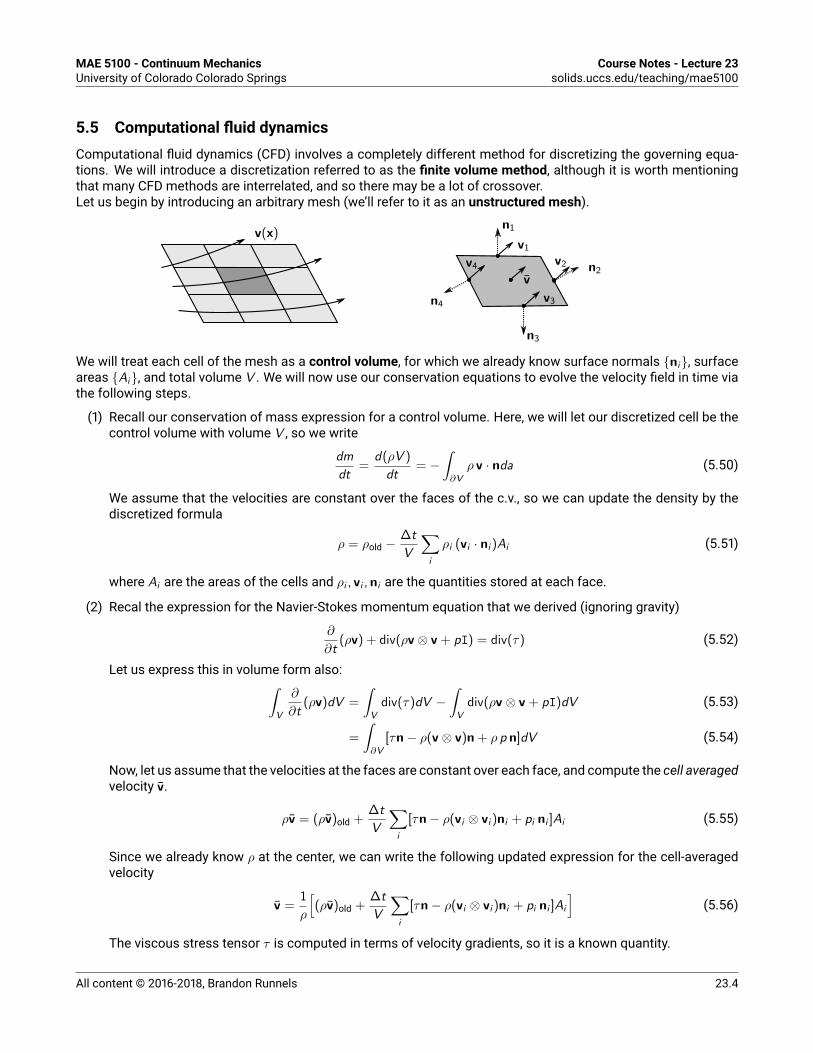
MAE 5100 - Continuum MechanicsUniversity of Colorado Colorado Springs Course Notes - Lecture 23solids.uccs.edu/teaching/mae5100
5.5 Computational fluid dynamicsComputational fluid dynamics (CFD) involves a completely different method for discretizing the governing equa-tions. We will introduce a discretization referred to as the finite volume method, although it is worth mentioningthat many CFD methods are interrelated, and so there may be a lot of crossover.Let us begin by introducing an arbitrary mesh (we’ll refer to it as an unstructured mesh).
v(x)n1
n2
n3
n4
v1
v2
v3
v4
v
We will treat each cell of the mesh as a control volume, for which we already know surface normals ni, surfaceareas Ai, and total volume V . We will now use our conservation equations to evolve the velocity field in time viathe following steps.(1) Recall our conservation of mass expression for a control volume. Here, we will let our discretized cell be thecontrol volume with volume V , so we write
dm
dt=
d(ρV )
dt= −
∫∂V
ρ v · nda (5.50)We assume that the velocities are constant over the faces of the c.v., so we can update the density by thediscretized formula
ρ = ρold − ∆t
V
∑i
ρi (vi · ni )Ai (5.51)where Ai are the areas of the cells and ρi , vi ,ni are the quantities stored at each face.
(2) Recal the expression for the Navier-Stokes momentum equation that we derived (ignoring gravity)∂
∂t(ρv) + div(ρv ⊗ v + pI) = div(τ) (5.52)
Let us express this in volume form also:∫V
∂
∂t(ρv)dV =
∫V
div(τ)dV −∫V
div(ρv ⊗ v + pI)dV (5.53)=
∫∂V
[τn− ρ(v ⊗ v)n + ρ p n]dV (5.54)Now, let us assume that the velocities at the faces are constant over each face, and compute the cell averagedvelocity v.
ρv = (ρv)old +∆t
V
∑i
[τn− ρ(vi ⊗ vi )ni + pi ni ]Ai (5.55)Since we already know ρ at the center, we can write the following updated expression for the cell-averagedvelocity
v =1
ρ
[(ρv)old +
∆t
V
∑i
[τn− ρ(vi ⊗ vi )ni + pi ni ]Ai
] (5.56)The viscous stress tensor τ is computed in terms of velocity gradients, so it is a known quantity.
All content © 2016-2018, Brandon Runnels 23.4
MAE 5100 - Continuum MechanicsUniversity of Colorado Colorado Springs Course Notes - Lecture 23solids.uccs.edu/teaching/mae5100
(3) We assume that we have a known equation of state, so we can use it to compute the updated pressure:p = p(ρ,T ) (5.57)
(4) Finally, we determine pressures pi, velocities vi, and densities ρi at the cell boundaries by interpolation.We note that this is a fully explicit scheme, in that it relies only on the current timestep’s values to find new ones.As a result, it cannot conserve energy completely. It is also a highly simplified scheme; there are much better waysof doing the above computation.For incompressible flow, special measures have to be taken to find the pressure field, since the equation of state isill-defined. One method of doing it is the fractional step or projection method, where the velocity field is estimated,then used to find a pressure field that is used to correct the original velocity field.
All content © 2016-2018, Brandon Runnels 23.5