mafs5030 quantitative modeling of derivative securities

1 MAFS5030 Quantitative Modeling of Derivative Securities

Tutorial Note 4

MAFS5030 Quantitative Modeling of Derivative Securities

Tutorial Note 4

Review on pricing technique in continuous time model (with multiple

assets)

In this tutorial, we shall review some important techniques in pricing derivatives

involving more than one stochastic random variables/ underlying assets. One difficulty

in pricing such derivatives is that the calculation involves the computation of

expectation involving several correlated random variables. One needs to employ various

methods/theorems so that one can compute the price in an easier way. The following

summarizes some useful theorems/methods for this purpose:

Girsanov Theorem (Describe the price dynamic of the underlying asset when the

probability measure is changed from 𝑃 to �̃�)

Numeraire invariance theorem (Describe the pricing formula of a contingent

claim when there is a change in numeraire)

Quanto prewashing technique (A method to determine the drift rate of the

target state variable under some probability measure in pricing quanto options).

Example 1 (Pricing of exchange options: A quick review)

We consider an exchange options (European) which the holder has the right to

exchange 𝐾 units of asset 𝑋 for one units of asset 𝑌. We let 𝑇 be the maturity date

of the options. The terminal payoff of the options is seen to be

𝑉𝑇(𝑋𝑇, 𝑌𝑇) = max(𝑌𝑇 − 𝐾𝑋𝑇 , 0), where 𝑋𝑇 and 𝑌𝑇 are prices of assets 𝑋 and 𝑌 at maturity date 𝑇 respectively. We

assume that the price processes of two assets are governed by

𝑑𝑋𝑡 = (𝑟 − 𝑞𝑋)𝑋𝑡𝑑𝑡 + 𝜎𝑋𝑋𝑡𝑑𝑍𝑋,𝑡𝑄 ,

𝑑𝑌𝑡 = (𝑟 − 𝑞𝑌)𝑌𝑡𝑑𝑡 + 𝜎𝑌𝑌𝑡𝑑𝑍𝑌,𝑡𝑄 ,

where 𝑍𝑋,𝑡𝑄 and 𝑍𝑌,𝑡

𝑄 are 𝑄-Brownian with 𝑑𝑍𝑋,𝑡𝑄 𝑑𝑍𝑌,𝑡

𝑄 = 𝜌𝑑𝑡.

Given the current prices of two assets 𝑋𝑡 and 𝑌𝑡, compute the current price of the

exchange options.

Solution

We take �̂�𝑡 = 𝑒𝑞𝑋𝑡𝑋𝑡 as the numeraire (recall that the asset 𝑋 pays continuous dividend

at the yield rate 𝑞𝑋). Using numeraire invariance theorem, the current price of the

exchange options can be expressed as


Tutorial Note 4

𝑉𝑡 = 𝑒−𝑟(𝑇−𝑡)𝔼𝑄[𝑉𝑇(𝑋𝑇 , 𝑌𝑇)|ℱ𝑡] = 𝑀𝑡𝔼

𝑄 [𝑉𝑇(𝑋𝑇, 𝑌𝑇)

𝑀𝑇|ℱ𝑡] = �̂�𝑡𝔼

𝑄𝑋 [𝑉𝑇(𝑋𝑇, 𝑌𝑇)

�̂�𝑇|ℱ𝑡]

= 𝑒𝑞𝑋𝑡𝑋𝑡𝔼𝑄𝑋 [

max(𝑌𝑇 − 𝐾𝑋𝑇 , 0)

𝑒𝑞𝑋𝑇𝑋𝑇|ℱ𝑡]

= 𝑋𝑡 𝑒−𝑞𝑋(𝑇−𝑡)𝔼𝑄𝑋 [max (

𝑌𝑇𝑋𝑇− 𝐾) |ℱ𝑡]

⏟ 𝑝𝑟𝑖𝑐𝑒 𝑜𝑓 𝑡ℎ𝑒 𝑒𝑥𝑐ℎ𝑎𝑛𝑔𝑒 𝑜𝑝𝑡𝑖𝑜𝑛𝑠 𝑎𝑡 𝑡𝑖𝑚𝑒 𝑡

(𝑚𝑒𝑎𝑠𝑢𝑟𝑒𝑑 𝑖𝑛 𝑢𝑛𝑖𝑡𝑠 𝑜𝑓 𝑎𝑠𝑠𝑒𝑡 𝑋)

……(∗)

To calculate the expectation 𝔼𝑄𝑋 [max (𝑌𝑇

𝑋𝑇− 𝐾) |ℱ𝑡], we need to know the

“distribution” of the random variable 𝑌𝑇

𝑋𝑇 under 𝑄𝑋.

By applying Ito’s lemma on the function 𝑓(𝑋𝑡, 𝑌𝑡) =𝑌𝑡

𝑋𝑡, we get

𝑑 (𝑌𝑡𝑋𝑡) =

[

(𝑟 − 𝑞𝑋)𝑋𝑡𝜕𝑓

𝜕𝑋𝑡+ (𝑟 − 𝑞𝑌)𝑌𝑡

𝜕𝑓

𝜕𝑌𝑡⏟

∑ 𝜇𝑖𝜕𝑓𝜕𝑋𝑖

𝑛𝑖=1

+1

2𝜎𝑋2𝑋𝑡

2𝜕2𝑓

𝜕𝑋𝑡2 + 𝜌𝜎𝑋𝜎𝑌𝑋𝑡𝑌𝑡

𝜕2𝑓

𝜕𝑋𝑡𝜕𝑌𝑡+1

2𝜎𝑌2𝑌𝑡

2𝜕2𝑓

𝜕𝑌𝑡2

⏟ 12∑ ∑ 𝜎𝑖𝜎𝑗

𝜕2𝑓𝜕𝑋𝑖𝜕𝑋𝑗

𝑛𝑗=1

𝑛𝑖=1 ]

𝑑𝑡 + 𝜎𝑋𝑋𝑡𝜕𝑓

𝜕𝑋𝑡𝑑𝑍𝑋,𝑡

𝑄

+ 𝜎𝑌𝑌𝑡𝜕𝑓

𝜕𝑌𝑡𝑑𝑍𝑌,𝑡

𝑄 .

⇒ 𝑑 (𝑌𝑡𝑋𝑡) = [(𝑟 − 𝑞𝑋)𝑋𝑡 (−

𝑌𝑡

𝑋𝑡2) + (𝑟 − 𝑞𝑌)𝑌𝑡 (

1

𝑋𝑡) +

1

2𝜎𝑋2𝑋𝑡

2 (2𝑌𝑡

𝑋𝑡3)

+ 𝜌𝜎𝑋𝜎𝑌𝑋𝑡𝑌𝑡 (−1

𝑋𝑡2) +

1

2𝜎𝑌2𝑌𝑡

2(0)] 𝑑𝑡 + 𝜎𝑋𝑋𝑡 (−𝑌𝑡

𝑋𝑡2)𝑑𝑍𝑋,𝑡

𝑄

+ 𝜎𝑌𝑌𝑡 (1

𝑋𝑡)𝑑𝑍𝑌,𝑡

𝑄

⇒ 𝑑 (𝑌𝑡𝑋𝑡) = [(𝑟 − 𝑞𝑌) − (𝑟 − 𝑞𝑋) + 𝜎𝑋

2 − 𝜌𝜎𝑋𝜎𝑌]𝑌𝑡𝑋𝑡𝑑𝑡 − 𝜎𝑋

𝑌𝑡𝑋𝑡𝑑𝑍𝑋,𝑡

𝑄 + 𝜎𝑌𝑌𝑡𝑋𝑡𝑑𝑍𝑌,𝑡

𝑄

By taking 𝑊𝑡 =𝑌𝑡

𝑋𝑡, we get

Unfortunately, the above equation is not useful because the random variables 𝑍𝑋,𝑡𝑄 and

𝑍𝑌,𝑡𝑄 are no longer to be the Brownian motion under 𝑄𝑋.

Step 1: Compute the price dynamic of 𝑌𝑡/𝑋𝑡

𝑑𝑊𝑡 = [(𝑟 − 𝑞𝑌) − (𝑟 − 𝑞𝑋) + 𝜎𝑋2 − 𝜌𝜎𝑋𝜎𝑌]𝑊𝑡𝑑𝑡 − 𝜎𝑋𝑊𝑡𝑑𝑍𝑋,𝑡

𝑄 + 𝜎𝑌𝑊𝑡𝑑𝑍𝑌,𝑡𝑄


Tutorial Note 4

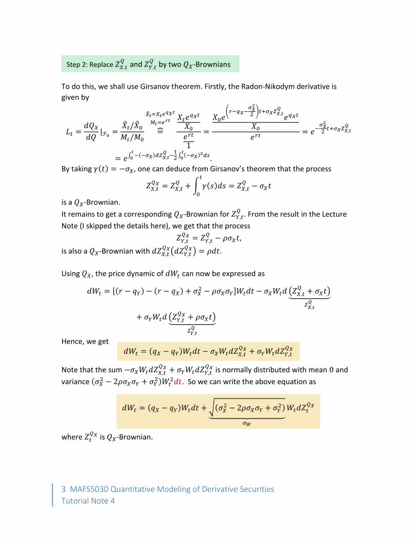
To do this, we shall use Girsanov theorem. Firstly, the Radon-Nikodym derivative is

given by

𝐿𝑡 =𝑑𝑄𝑋𝑑𝑄

|ℱ0 =�̂�𝑡/�̂�0𝑀𝑡/𝑀0

=⏞

�̂�𝑡=𝑋𝑡𝑒𝑞𝑋𝑡

𝑀𝑡=𝑒𝑟𝑡 𝑋𝑡𝑒

𝑞𝑋𝑡

𝑋0𝑒𝑟𝑡

1

=

𝑋0𝑒(𝑟−𝑞𝑋−

𝜎𝑋2

2)𝑡+𝜎𝑋𝑍𝑋,𝑡

𝑄

𝑒𝑞𝑋𝑡

𝑋0𝑒𝑟𝑡

= 𝑒−𝜎𝑋2

2𝑡+𝜎𝑋𝑍𝑋,𝑡

𝑄

= 𝑒∫ −(−𝜎𝑋)𝑑𝑍𝑋,𝑡𝑄𝑡

0−12∫

(−𝜎𝑋)2𝑑𝑠

𝑡0 .

By taking 𝛾(𝑡) = −𝜎𝑋, one can deduce from Girsanov’s theorem that the process

𝑍𝑋,𝑡𝑄𝑋 = 𝑍𝑋,𝑡

𝑄 +∫ 𝛾(𝑠)𝑑𝑠𝑡

0

= 𝑍𝑋,𝑡𝑄 − 𝜎𝑋𝑡

is a 𝑄𝑋-Brownian.

It remains to get a corresponding 𝑄𝑋-Brownian for 𝑍𝑌,𝑡𝑄 . From the result in the Lecture

Note (I skipped the details here), we get that the process

𝑍𝑌,𝑡𝑄𝑋 = 𝑍𝑌,𝑡

𝑄 − 𝜌𝜎𝑋𝑡,

is also a 𝑄𝑋-Brownian with 𝑑𝑍𝑋,𝑡𝑄𝑋(𝑑𝑍𝑌,𝑡

𝑄𝑋) = 𝜌𝑑𝑡.

Using 𝑄𝑋, the price dynamic of 𝑑𝑊𝑡 can now be expressed as

𝑑𝑊𝑡 = [(𝑟 − 𝑞𝑌) − (𝑟 − 𝑞𝑋) + 𝜎𝑋2 − 𝜌𝜎𝑋𝜎𝑌]𝑊𝑡𝑑𝑡 − 𝜎𝑋𝑊𝑡𝑑 (𝑍𝑋,𝑡

𝑄 + 𝜎𝑋𝑡)⏟

𝑍𝑋,𝑡𝑄

+ 𝜎𝑌𝑊𝑡𝑑 (𝑍𝑌,𝑡𝑄𝑋 + 𝜌𝜎𝑋𝑡)⏟

𝑍𝑌,𝑡𝑄

Hence, we get

Note that the sum −𝜎𝑋𝑊𝑡𝑑𝑍𝑋,𝑡𝑄𝑋 + 𝜎𝑌𝑊𝑡𝑑𝑍𝑌,𝑡

𝑄𝑋 is normally distributed with mean 0 and

variance (𝜎𝑋2 − 2𝜌𝜎𝑋𝜎𝑌 + 𝜎𝑌

2)𝑊𝑡2𝑑𝑡. So we can write the above equation as

where 𝑍𝑡𝑄𝑋 is 𝑄𝑋-Brownian.

Step 2: Replace 𝑍𝑋,𝑡𝑄 and 𝑍𝑌,𝑡

𝑄 by two 𝑄𝑋-Brownians

𝑑𝑊𝑡 = (𝑞𝑋 − 𝑞𝑌)𝑊𝑡𝑑𝑡 − 𝜎𝑋𝑊𝑡𝑑𝑍𝑋,𝑡𝑄𝑋 + 𝜎𝑌𝑊𝑡𝑑𝑍𝑌,𝑡

𝑄𝑋

𝑑𝑊𝑡 = (𝑞𝑋 − 𝑞𝑌)𝑊𝑡𝑑𝑡 + √(𝜎𝑋2 − 2𝜌𝜎𝑋𝜎𝑌 + 𝜎𝑌

2)⏟

𝜎𝑊

𝑊𝑡𝑑𝑍𝑡𝑄𝑋


Tutorial Note 4

Given the current value of 𝑋𝑡, 𝑌𝑡 (so that 𝑊𝑡 =𝑌𝑡

𝑋𝑡 is known), the value of 𝑊𝑇 at maturity

date 𝑇 can now be expressed as

𝑊𝑇 = 𝑊𝑡𝑒(𝑞𝑋−𝑞𝑌−

𝜎𝑊2

2)(𝑇−𝑡)+𝜎𝑊𝑍𝑇−𝑡

𝑄𝑋

.

Note that

𝑊𝑇 =𝑌𝑇𝑋𝑇> 𝐾 ⇔ 𝑍𝑇−𝑡

𝑄𝑋 >ln𝐾𝑊𝑡− (𝑞𝑋 − 𝑞𝑌 −

𝜎𝑊2

2 )(𝑇 − 𝑡)

𝜎𝑊⏟ 𝑑𝑒𝑛𝑜𝑡𝑒𝑑 𝑏𝑦 𝑑

From equation (∗), the time-𝑡 price of the exchange options can now be expressed as

𝑉𝑡 = 𝑋𝑡𝑒−𝑞𝑋(𝑇−𝑡)𝔼𝑄𝑋 [max (

𝑌𝑇𝑋𝑇− 𝐾) |ℱ𝑡] = 𝑋𝑡𝑒

−𝑞𝑋(𝑇−𝑡)𝔼𝑄𝑋[max(𝑊𝑇 − 𝐾) |ℱ𝑡]

= 𝑋𝑡𝑒−𝑞𝑋(𝑇−𝑡) [∫ (𝑊𝑡𝑒

(𝑞𝑋−𝑞𝑌−𝜎𝑊2

2)(𝑇−𝑡)+𝜎𝑊𝑧

−𝐾)(1

√2𝜋(𝑇 − 𝑡)𝑒−

𝑧2

2(𝑇−𝑡))𝑑𝑧∞

𝑑

+∫ (0) (1

√2𝜋(𝑇 − 𝑡)𝑒−

𝑧2

2(𝑇−𝑡))𝑑𝑧𝑑

−∞

]

= 𝑋𝑡𝑒−𝑞𝑋(𝑇−𝑡) [∫ 𝑊𝑡𝑒

(𝑞𝑋−𝑞𝑌−𝜎𝑊2

2)(𝑇−𝑡)+𝜎𝑊𝑧

(1

√2𝜋(𝑇 − 𝑡)𝑒−

𝑧2


𝑑

− 𝐾∫ (1

√2𝜋(𝑇 − 𝑡)𝑒−

𝑧2


𝑑

]

= 𝑋𝑡𝑒−𝑞𝑋(𝑇−𝑡) [𝑊𝑡𝑒

(𝑞𝑋−𝑞𝑌)(𝑇−𝑡)∫ (1

√2𝜋(𝑇 − 𝑡)𝑒−(𝑧−𝜎𝑊(𝑇−𝑡))

2

2(𝑇−𝑡) )𝑑𝑧∞

𝑑

− 𝐾∫ (1

√2𝜋(𝑇 − 𝑡)𝑒−12(

𝑧

√𝑇−𝑡)2

)𝑑𝑧∞

𝑑

]

=⏞

𝑧1=𝑧−𝜎𝑊(𝑇−𝑡)

√𝑇−𝑡

𝑧2=𝑧

√𝑇−𝑡

𝑋𝑡𝑒−𝑞𝑋(𝑇−𝑡) [𝑊𝑡𝑒

(𝑞𝑋−𝑞𝑌)(𝑇−𝑡)∫ (1

√2𝜋𝑒−

𝑧12

2 )𝑑𝑧1

∞

𝑑−𝜎𝑊(𝑇−𝑡)

√𝑇−𝑡

− 𝐾∫ (1

√2𝜋𝑒−

𝑧22 )𝑑𝑧2

∞

𝑑

√𝑇−𝑡

]

Step 3: Obtain the price process of 𝑊𝑡 under 𝑄𝑋

Step 4: Obtain the pricing formula


Tutorial Note 4

= 𝑋𝑡𝑒−𝑞𝑋(𝑇−𝑡)𝑊𝑡𝑒

(𝑞𝑋−𝑞𝑌)(𝑇−𝑡) [1 − 𝑁 (𝑑 − 𝜎𝑊(𝑇 − 𝑡)

√𝑇 − 𝑡)]

− 𝐾𝑋𝑡𝑒−𝑞𝑋(𝑇−𝑡) [1 − 𝑁 (

𝑑

√𝑇 − 𝑡)]

= 𝑋𝑡𝑒−𝑞𝑋(𝑇−𝑡) (

𝑌𝑡𝑋𝑡) 𝑒(𝑞𝑋−𝑞𝑌)(𝑇−𝑡) [𝑁 (−

𝑑 − 𝜎𝑊(𝑇 − 𝑡)

√𝑇 − 𝑡)]

− 𝐾𝑋𝑡𝑒−𝑞𝑋(𝑇−𝑡) [𝑁 (−

𝑑

√𝑇 − 𝑡)]

= 𝑌𝑡𝑒−𝑞𝑌(𝑇−𝑡)𝑁(𝑑1) − 𝐾𝑋𝑡𝑒

−𝑞𝑋(𝑇−𝑡)𝑁(𝑑2),

where

𝑑1 = −𝑑 − 𝜎𝑊(𝑇 − 𝑡)

√𝑇 − 𝑡=ln (

𝑌𝑡𝐾𝑋𝑡

) + (𝑞𝑋 − 𝑞𝑌 +𝜎𝑊2

2 )(𝑇 − 𝑡)

𝜎𝑊√𝑇 − 𝑡

𝑑2 = −𝑑

√𝑇 − 𝑡=ln (

𝑌𝑡𝐾𝑋𝑡

) + (𝑞𝑋 − 𝑞𝑌 −𝜎𝑊2

2 )(𝑇 − 𝑡)

𝜎𝑊√𝑇 − 𝑡

Example 2 (Quantos digital options)

(a) We consider a quanto on a foreign currency denominated asset which pays

holder an amount 𝐹𝑇 (1 unit of foreign currency) at the maturity date 𝑇 if the

asset price 𝑆𝑇 is above 𝑋𝑓 and nothing if otherwise. So the terminal payoff of

the options can be expressed as

𝑉𝑇(𝑆𝑇, 𝐹𝑇) = {𝐹𝑇 𝑖𝑓 𝑆𝑇 ≥ 𝑋𝑓

0 𝑖𝑓 𝑆𝑇 < 𝑋𝑓.

Here, 𝐹𝑇 denotes the exchange rate for the foreign currency and 𝑆𝑇 is the

price (measured in foreign currency) of the underlying asset. We assume that

both 𝐹𝑇 and 𝑆𝑇 are governing by Geometric Brownian motion.

Given the value of 𝐹𝑡 and 𝑆𝑡, what is the time-𝑡 price of the options?

(b) We consider a quanto on a foreign currency denominated asset which pays

holder an amount 𝐹𝑇 (1 unit of foreign currency) at the maturity date 𝑇 if the

asset price 𝑆𝑇 is above 𝑋𝑓 and nothing if otherwise. So the terminal payoff of

the options can be expressed as

𝑉𝑇(𝑆𝑇, 𝐹𝑇) = {1 𝑖𝑓 𝑆𝑇 ≥ 𝑋𝑓

0 𝑖𝑓 𝑆𝑇 < 𝑋𝑓.

Here, 𝐹𝑇 denotes the exchange rate for the foreign currency and 𝑆𝑇 is the

price (measured in foreign currency) of the underlying asset. What is the

corresponding time-𝑡 price of the options?


Tutorial Note 4

Some notations:

We let 𝑄𝑑 and 𝑄𝑓 be the risk neutral probability measure under domestic

currency and foreign currency respectively.

We let 𝑟𝑑 and 𝑟𝑓 be the risk-free interest rate of domestic currency and foreign

currency respectively.

Solution of (a)

Assuming the options is attainable, the time-𝑡 price of the quanto options can be

expressed, using risk neutral valuation principle, as

𝑉𝑡(𝑆𝑡, 𝐹𝑡) = 𝑒−𝑟𝑑(𝑇−𝑡)𝔼𝑄𝑑[𝑉𝑇(𝑆𝑇, 𝐹𝑇)|ℱ𝑡] = 𝑒

−𝑟𝑑(𝑇−𝑡)𝔼𝑄𝑑 [𝐹𝑇𝟏{𝑆𝑇>𝑋𝑓}|ℱ𝑡].

We take 𝑁(𝑡) = 𝑒𝑟𝑓𝑡𝐹𝑡 as the numeraire (*Here, 𝑁𝑡 is the value of one unit of foreign

currency bought at time 0). Using numeraire invariance theorem, we deduce that

𝑉𝑡(𝑆𝑡, 𝐹𝑡) = 𝑒−𝑟𝑑(𝑇−𝑡)𝔼𝑄𝑑 [𝐹𝑇𝟏{𝑆𝑇>𝑋𝑓}|ℱ𝑡] =⏞

𝑀𝑑(𝑡)=𝑒𝑟𝑑𝑡

𝑀𝑑(𝑡)

𝑀𝑑(𝑇)𝔼𝑄𝑑 [𝐹𝑇𝟏{𝑆𝑇>𝑋𝑓}|ℱ𝑡]

= 𝑀𝑑(𝑡)𝔼𝑄𝑑 [

𝐹𝑇𝟏{𝑆𝑇>𝑋𝑓}

𝑀𝑑(𝑇)|ℱ𝑡] =

(∗) 𝑁(𝑡)𝔼𝑄𝑓 [𝐹𝑇𝟏{𝑆𝑇>𝑋𝑓}

𝑁(𝑇)|ℱ𝑡]

= 𝑒𝑟𝑓𝑡𝐹𝑡𝔼𝑄𝑓 [

𝐹𝑇𝟏{𝑆𝑇>𝑋𝑓}

𝑒𝑟𝑓𝑇𝐹𝑇|ℱ𝑡] = 𝑒

−𝑟𝑓(𝑇−𝑡)𝐹𝑡𝔼𝑄𝑓 [𝟏{𝑆𝑇>𝑋𝑓}|ℱ𝑡].

So we get

To calculate the expectation, we need to obtain the price dynamic of 𝑆𝑇 under the

probability measure 𝑄𝑓.

Since 𝑆𝑡 is assumed to follow Geometric Brownian Motion and its value is in foreign

currency, so under risk neutral probability measure 𝑄𝑓 (in foreign currency world), 𝑆𝑡

should follow:

Here, 𝑞 is dividend yield rate of the asset (𝑞 = 0 if the asset is non-dividend paying) and

𝜎𝑆 is the volatility of the asset.

IDEA: It may be difficult to compute the expectation directly since we need to

handle two correlated random variables (𝐹𝑇 , 𝑆𝑇) simultaneously. The computation

would be easier if we apply change of numeraire technical by taking the foreign

currency as the numeraire.

𝑉𝑡(𝑆𝑡, 𝐹𝑡) = 𝑒−𝑟𝑓(𝑇−𝑡)𝐹𝑡𝔼

𝑄𝑓 [𝟏{𝑆𝑇>𝑋𝑓}|ℱ𝑡]

𝑑𝑆𝑡 = (𝑟𝑓 − 𝑞)𝑆𝑡𝑑𝑡 + 𝜎𝑆𝑆𝑡𝑑𝑍𝑡𝑄𝑓 .


Tutorial Note 4

Given the current value of 𝑆𝑡, the asset price at the maturity date can be expressed as

𝑆𝑇 = 𝑆𝑡𝑒(𝑟𝑓−𝑞−

𝜎𝑆2

2)(𝑇−𝑡)+𝜎𝑆𝑍𝑇−𝑡

𝑄𝑓

.

Together with the fact that 𝑍𝑇−𝑡𝑄𝑓 is normally distributed with mean 0 and variance 𝑇 − 𝑡

and the fact that

𝑆𝑇 > 𝑋𝑓 ⇔ 𝑍𝑇−𝑡𝑄𝑓 >

ln𝑋𝑓𝑆𝑡− (𝑟𝑓 − 𝑞 −

𝜎𝑆2

2 )(𝑇 − 𝑡)

𝜎𝑆⏟ 𝑑

the expectation can be computed as

𝔼𝑄𝑓 [𝟏{𝑆𝑇>𝑋𝑓}|ℱ𝑡] = ∫ (1)1

√2𝜋(𝑇 − 𝑡)𝑒−

𝑧2

2(𝑇−𝑡)𝑑𝑧∞

𝑑

=⏞

𝑦=𝑧

√𝑇−𝑡

∫1

√2𝜋𝑒−

𝑦2

2 𝑑𝑦∞

𝑑

√𝑇−𝑡

= 1 − 𝑁 (𝑑

√𝑇 − 𝑡) = 𝑁 (−

𝑑

√𝑇 − 𝑡)

= 𝑁

(

ln𝑆𝑡𝑋𝑓+ (𝑟𝑓 − 𝑞 −

𝜎𝑆2

2 )(𝑇 − 𝑡)

𝜎𝑆√𝑇 − 𝑡⏟ =𝑑1 )

.

Hence, the time-𝑡 price of the quanto options is


𝑄𝑓 [𝟏{𝑆𝑇>𝑋𝑓}|ℱ𝑡] = 𝑒−𝑟𝑓(𝑇−𝑡)𝐹𝑡𝑁(𝑑1).

Solution of (b)

Using risk neutral valuation principle, the time-𝑡 price of the quanto options can be

expressed, using risk neutral valuation principle, as

𝑉𝑡(𝑆𝑡, 𝐹𝑡) = 𝑒−𝑟𝑑(𝑇−𝑡)𝔼𝑄𝑑[𝑉𝑇(𝑆𝑇, 𝐹𝑇)|ℱ𝑡] = 𝑒

−𝑟𝑑(𝑇−𝑡)𝔼𝑄𝑑 [𝟏{𝑆𝑇>𝑋𝑓}|ℱ𝑡].

Recall that the price dynamic of 𝑆𝑇 under 𝑄𝑓 is

𝑑𝑆𝑡𝑆𝑡= (𝑟𝑓 − 𝑞)𝑑𝑡 + 𝜎𝑆𝑑𝑍𝑆,𝑡

𝑄𝑓 .

Using Girsanov’s theorem, the corresponding price process of 𝑆𝑇 under 𝑄𝑑 is given by 𝑑𝑆𝑡𝑆𝑡= 𝛿𝑆

𝑑𝑑𝑡 + 𝜎𝑆𝑑𝑍𝑆,𝑡𝑄𝑑 .

Here, 𝑍𝑆,𝑡𝑄𝑑 is standard Brownian motion under 𝑄𝑑.

IDEA: To calculate the expectation, we need to obtain the price dynamic of 𝑆𝑇

under 𝑄𝑑 (in domestic world). To do so, we shall apply the quanto prewashing

technique.


Tutorial Note 4

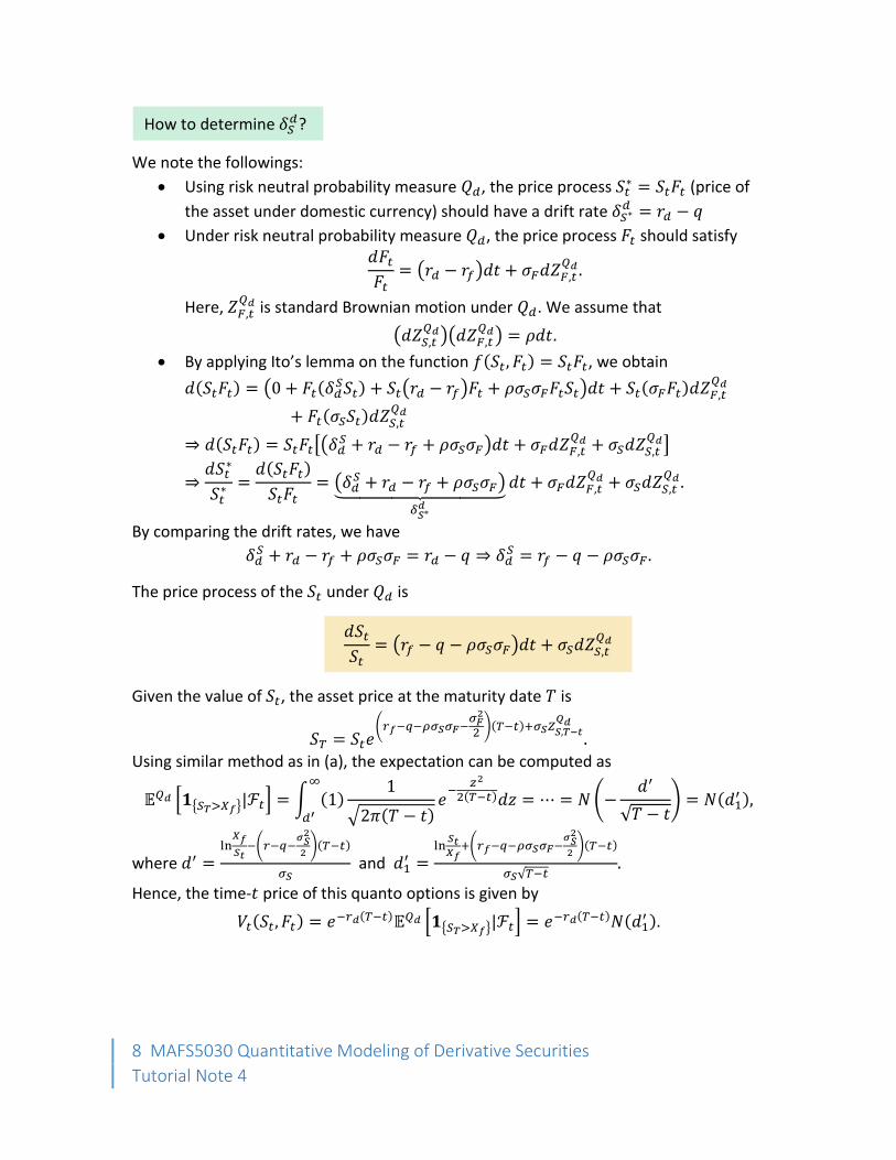
We note the followings:

Using risk neutral probability measure 𝑄𝑑, the price process 𝑆𝑡∗ = 𝑆𝑡𝐹𝑡 (price of

the asset under domestic currency) should have a drift rate 𝛿𝑆∗𝑑 = 𝑟𝑑 − 𝑞

Under risk neutral probability measure 𝑄𝑑, the price process 𝐹𝑡 should satisfy 𝑑𝐹𝑡𝐹𝑡= (𝑟𝑑 − 𝑟𝑓)𝑑𝑡 + 𝜎𝐹𝑑𝑍𝐹,𝑡

𝑄𝑑 .

Here, 𝑍𝐹,𝑡𝑄𝑑 is standard Brownian motion under 𝑄𝑑. We assume that

(𝑑𝑍𝑆,𝑡𝑄𝑑)(𝑑𝑍𝐹,𝑡

𝑄𝑑) = 𝜌𝑑𝑡.

By applying Ito’s lemma on the function 𝑓(𝑆𝑡, 𝐹𝑡) = 𝑆𝑡𝐹𝑡, we obtain

𝑑(𝑆𝑡𝐹𝑡) = (0 + 𝐹𝑡(𝛿𝑑𝑆𝑆𝑡) + 𝑆𝑡(𝑟𝑑 − 𝑟𝑓)𝐹𝑡 + 𝜌𝜎𝑆𝜎𝐹𝐹𝑡𝑆𝑡)𝑑𝑡 + 𝑆𝑡(𝜎𝐹𝐹𝑡)𝑑𝑍𝐹,𝑡

𝑄𝑑

+ 𝐹𝑡(𝜎𝑆𝑆𝑡)𝑑𝑍𝑆,𝑡𝑄𝑑

⇒ 𝑑(𝑆𝑡𝐹𝑡) = 𝑆𝑡𝐹𝑡[(𝛿𝑑𝑆 + 𝑟𝑑 − 𝑟𝑓 + 𝜌𝜎𝑆𝜎𝐹)𝑑𝑡 + 𝜎𝐹𝑑𝑍𝐹,𝑡

𝑄𝑑 + 𝜎𝑆𝑑𝑍𝑆,𝑡𝑄𝑑]

⇒𝑑𝑆𝑡

∗

𝑆𝑡∗ =

𝑑(𝑆𝑡𝐹𝑡)

𝑆𝑡𝐹𝑡= (𝛿𝑑

𝑆 + 𝑟𝑑 − 𝑟𝑓 + 𝜌𝜎𝑆𝜎𝐹)⏟ 𝛿𝑆∗𝑑

𝑑𝑡 + 𝜎𝐹𝑑𝑍𝐹,𝑡𝑄𝑑 + 𝜎𝑆𝑑𝑍𝑆,𝑡

𝑄𝑑 .

By comparing the drift rates, we have

𝛿𝑑𝑆 + 𝑟𝑑 − 𝑟𝑓 + 𝜌𝜎𝑆𝜎𝐹 = 𝑟𝑑 − 𝑞 ⇒ 𝛿𝑑

𝑆 = 𝑟𝑓 − 𝑞 − 𝜌𝜎𝑆𝜎𝐹.

The price process of the 𝑆𝑡 under 𝑄𝑑 is

Given the value of 𝑆𝑡, the asset price at the maturity date 𝑇 is

𝑆𝑇 = 𝑆𝑡𝑒(𝑟𝑓−𝑞−𝜌𝜎𝑆𝜎𝐹−

𝜎𝐹2

2)(𝑇−𝑡)+𝜎𝑆𝑍𝑆,𝑇−𝑡

𝑄𝑑

.

Using similar method as in (a), the expectation can be computed as

𝔼𝑄𝑑 [𝟏{𝑆𝑇>𝑋𝑓}|ℱ𝑡] = ∫ (1)1

√2𝜋(𝑇 − 𝑡)𝑒−

𝑧2

2(𝑇−𝑡)𝑑𝑧∞

𝑑′= ⋯ = 𝑁(−

𝑑′

√𝑇 − 𝑡) = 𝑁(𝑑1

′ ),

where 𝑑′ =ln𝑋𝑓

𝑆𝑡−(𝑟−𝑞−

𝜎𝑆2

2)(𝑇−𝑡)

𝜎𝑆 and 𝑑1

′ =ln𝑆𝑡𝑋𝑓+(𝑟𝑓−𝑞−𝜌𝜎𝑆𝜎𝐹−

𝜎𝑆2

2)(𝑇−𝑡)

𝜎𝑆√𝑇−𝑡.

Hence, the time-𝑡 price of this quanto options is given by

𝑉𝑡(𝑆𝑡, 𝐹𝑡) = 𝑒−𝑟𝑑(𝑇−𝑡)𝔼𝑄𝑑 [𝟏{𝑆𝑇>𝑋𝑓}|ℱ𝑡] = 𝑒

−𝑟𝑑(𝑇−𝑡)𝑁(𝑑1′ ).

How to determine 𝛿𝑆𝑑?

𝑑𝑆𝑡𝑆𝑡= (𝑟𝑓 − 𝑞 − 𝜌𝜎𝑆𝜎𝐹)𝑑𝑡 + 𝜎𝑆𝑑𝑍𝑆,𝑡

𝑄𝑑


Tutorial Note 4

Example 3 (Two more examples on quanto options: A quick review)

(a) We consider a foreign equity call struck which the terminal payoff is given by

𝑉𝑇 = 𝐹𝑇max(𝑆𝑇 − 𝑋𝑓, 0).

Find the time-𝑡 price of the quanto options.

(b) We consider a fixed exchange rate foreign equity call which the terminal

payoff is given by

𝑉𝑇 = 𝐹0max(𝑆𝑇 − 𝑋𝑓, 0),

Where 𝐹0 is the predetermined fixed exchange rate. Find the time-𝑡 price of

the quanto options.

(*The notations used in this example is same as those used in Example 2)

Solution of (a)

The time-𝑡 price of the quanto options can be expressed, using risk neutral valuation

principle, as

𝑉𝑡(𝑆𝑡, 𝐹𝑡) = 𝑒−𝑟𝑑(𝑇−𝑡)𝔼𝑄𝑑[𝑉𝑇(𝑆𝑇 , 𝐹𝑇)|ℱ𝑡] = 𝑒

−𝑟𝑑(𝑇−𝑡)𝔼𝑄𝑑[𝐹𝑇max(𝑆𝑇 − 𝑋𝑓, 0) |ℱ𝑡].

Since the expectation involves two random variables, one shall simplify the expectation

using change of numeraire technique (take foreign currency 𝐹𝑡 as numeraire).

We take 𝑁𝑡 = 𝑒𝑟𝑓𝑡𝐹𝑡 as our numeraire. By numeraire invariance theorem, we deduce

that

𝑉𝑡(𝑆𝑡, 𝐹𝑡) = 𝑒−𝑟𝑑(𝑇−𝑡)𝔼𝑄𝑑[𝐹𝑇max(𝑆𝑇 − 𝑋𝑓 , 0) |ℱ𝑡]

=⏞𝑀𝑡=𝑒

𝑟𝑡𝑀𝑡𝑀𝑇

𝔼𝑄𝑑[𝐹𝑇max(𝑆𝑇 − 𝑋𝑓, 0) |ℱ𝑡]

= 𝑀𝑡𝔼𝑄𝑑 [

𝐹𝑇max(𝑆𝑇 − 𝑋𝑓 , 0)

𝑀𝑇|ℱ𝑡]

= 𝑁𝑡𝔼𝑄𝑓 [


𝑁𝑇|ℱ𝑡] = 𝑒

𝑟𝑓𝑡𝐹𝑡𝔼𝑄𝑓 [


𝑒𝑟𝑓𝑇𝐹𝑇|ℱ𝑡]

= 𝑒−𝑟𝑓(𝑇−𝑡)𝐹𝑡𝔼𝑄𝑓[max(𝑆𝑇 − 𝑋𝑓 , 0) |ℱ𝑡].

So we get

To calculate the above expectation, we observe that the term 𝑒−𝑟𝑓(𝑇−𝑡)𝔼𝑄𝑓[max(𝑆𝑇 −

𝑋𝑓 , 0) |ℱ𝑡] is simply the time-𝑡 price of the European call option on the foreign asset in

foreign currency. So we have

𝑒−𝑟𝑓(𝑇−𝑡)𝔼𝑄𝑓[max(𝑆𝑇 − 𝑋𝑓 , 0) |ℱ𝑡] = 𝑐𝑓(𝑆, 𝑡)

= 𝑆𝑡𝑒−𝑞(𝑇−𝑡)𝑁(𝑑1) − 𝑋𝑓𝑒

−𝑟𝑓(𝑇−𝑡)𝑁(𝑑2),


𝑄𝑓[max(𝑆𝑇 − 𝑋𝑓 , 0) |ℱ𝑡]


Tutorial Note 4

where

𝑑1 =

ln𝑆𝑡𝑋𝑓+ (𝑟𝑓 − 𝑞 +

𝜎𝑆2

2 )(𝑇 − 𝑡)

𝜎𝑆√𝑇 − 𝑡, 𝑑2 = 𝑑1 − 𝜎𝑆√𝑇 − 𝑡.

Solution of (b)

The time-𝑡 price of the quanto options can be expressed, using risk neutral valuation

principle, as

𝑉𝑡(𝑆𝑡, 𝐹𝑡) = 𝑒−𝑟𝑑(𝑇−𝑡)𝔼𝑄𝑑[𝑉𝑇(𝑆𝑇 , 𝐹𝑇)|ℱ𝑡] = 𝑒

−𝑟𝑑(𝑇−𝑡)𝔼𝑄𝑑[𝐹0max(𝑆𝑇 − 𝑋𝑓 , 0) |ℱ𝑡].

Since there is only one random variable in the expectation, we can compute the

expectation directly without using change of numeraire.

To compute the expectation, one needs to obtain the price dynamic of 𝑆𝑡 under risk

neutral probability measure 𝑄𝑑 (not 𝑄𝑓).

Using similar method as in Example 2(b), we get

Given the current value of 𝑆𝑡, the value of 𝑆𝑇 can be expressed as

𝑆𝑇 = 𝑆𝑡𝑒(𝛿𝑆

𝑑−𝜎𝑆2

2)(𝑇−𝑡)+𝜎𝑆𝑍𝑆,𝑇−𝑡

𝑄𝑑

. Note that

𝑆𝑇 > 𝑋 ⇔ 𝑍𝑆,𝑇−𝑡𝑄𝑑 >

ln𝑋𝑆𝑡− (𝛿𝑆

𝑑 −𝜎𝑆2

2 )(𝑇 − 𝑡)

𝜎𝑆⏟ 𝑑

.

Together with the fact that 𝑍𝑆,𝑇−𝑡𝑄𝑑 is normally distributed with mean 0 and variance 𝑇 −

𝑡, the fair price can be computed as

𝑉𝑡(𝑆𝑡, 𝐹𝑡) = 𝑒−𝑟𝑑(𝑇−𝑡)𝔼𝑄𝑑[𝐹0max(𝑆𝑇 − 𝑋𝑓, 0) |ℱ𝑡]

= 𝐹0𝑒−𝑟𝑑(𝑇−𝑡) [∫ (𝑆𝑡𝑒

(𝛿𝑆𝑑−𝜎𝑆2

2)(𝑇−𝑡)+𝜎𝑆𝑧

− 𝑋𝑓)(1

√2𝜋(𝑇 − 𝑡)𝑒−

𝑧2


𝑑

]

= ⋯ = 𝐹0𝑒−𝑟𝑑(𝑇−𝑡) [𝑆𝑒𝛿𝑆

𝑑(𝑇−𝑡)𝑁(𝑑1) − 𝑋𝑓𝑁(𝑑2)],

where

𝑑1 =

ln𝑆𝑡𝑋𝑓+ (𝛿𝑆

𝑑 +𝜎𝑆2

2 )(𝑇 − 𝑡)

𝜎𝑆√𝑇 − 𝑡, 𝑑2 = 𝑑1 − 𝜎𝑆√𝑇 − 𝑡.

𝑑𝑆𝑡𝑆𝑡= 𝛿𝑆

𝑑𝑑𝑡 + 𝜎𝑆𝑑𝑍𝑆,𝑡𝑄𝑑 = (𝑟𝑓 − 𝑞 − 𝜌𝜎𝑆𝜎𝐹)𝑑𝑡 + 𝜎𝑆𝑑𝑍𝑆,𝑡

𝑄𝑑


Tutorial Note 4

Example 4 (Problem 4 of 2013 Final)

We let 𝐹𝑆\𝑈 = 𝐹𝑆\𝑈(𝑡) denote the Singaporean currency price of 1 unit of US

currency and 𝐹𝐻\𝑆 denote the Hong Kong currency price of 1 unit of Singaporean

currency.

Assume that 𝐹𝑆\𝑈 is governed by the following dynamics (GBM) under the risk

neutral measure 𝑄𝑆 in the Singaporean currency world: 𝑑𝐹𝑆\𝑈

𝐹𝑆\𝑈= (𝑟𝑆𝐺𝐷 − 𝑟𝑈𝑆𝐷)𝑑𝑡 + 𝜎𝐹𝑆\𝑈𝑑𝑍𝐹𝑆\𝑈

𝑄𝑆 ,

where 𝑍𝐹𝑆\𝑈𝑄𝑆 is the Brownian motion under 𝑄𝑆.

We consider a quanto option that pays 𝐹𝐻\𝑆 Hong Kong dollars if 𝐹𝑆\𝑈 is above the

strike price 𝑋. Find the value of the quanto option in Hong Kong currency in terms of

the riskless interest rates of different currency worlds and volatility values 𝜎𝐹𝑆\𝑈 and

𝜎𝐹𝐻\𝑆 .

Solution

We shall calculate the price of the quanto options by the following steps:

Using risk neutral valuation principle, the price of the quanto price (in HKD currency) is

given by

𝑉𝑡 = 𝑒−𝑟𝐻𝐾𝐷(𝑇−𝑡)𝔼𝑄

𝐻[𝑉𝑇|ℱ𝑡] = 𝑒

−𝑟𝐻𝐾𝐷(𝑇−𝑡)𝔼𝑄𝐻[𝐹𝐻\𝑆(𝑇)𝟏{𝐹𝑆\𝑈(𝑇)>𝑋}|ℱ𝑡].

Since the expectation involves two random variables, one needs to simplify the

expectation by applying “change of numeraire” technique.

Note that 𝐹𝐻\𝑆 represents the price of 1 unit of Singaporean currency in HKD currency.

We shall choose Singaporean currency as our new numeraire.

We take 𝑁𝑡 = 𝑒𝑟𝑆𝐺𝐷𝑡𝐹𝐻\𝑆(𝑡) as the numeriare. By numeraire invariance theorem, the

pricing formula can be expressed as


𝐻[𝐹𝐻\𝑆(𝑇)𝟏{𝐹𝑆\𝑈(𝑇)>𝑋}|ℱ𝑡]

=⏞𝑀𝑡=𝑒

𝑟𝐻𝐾𝐷𝑡𝑀𝑡𝑀𝑇

𝔼𝑄𝐻[𝐹𝐻\𝑆(𝑇)𝟏{𝐹𝑆\𝑈(𝑇)>𝑋}|ℱ𝑡]

= 𝑀𝑡𝔼𝑄𝐻 [

𝐹𝐻\𝑆(𝑇)

𝑀𝑇𝟏{𝐹𝑆\𝑈(𝑇)>𝑋}|ℱ𝑡] = 𝑁𝑡𝔼

𝑄𝑆 [𝐹𝐻\𝑆(𝑇)

𝑁𝑇𝟏{𝐹𝑆\𝑈(𝑇)>𝑋}|ℱ𝑡]

= 𝑒𝑟𝑆𝐺𝐷𝑡𝐹𝐻\𝑆(𝑡)𝔼𝑄𝑆 [

𝐹𝐻\𝑆(𝑇)

𝑒𝑟𝑆𝐺𝐷𝑇𝐹𝐻\𝑆(𝑇)𝟏{𝐹𝑆\𝑈(𝑇)>𝑋}|ℱ𝑡]

= 𝑒−𝑟𝑆𝐺𝐷(𝑇−𝑡)𝐹𝐻\𝑆(𝑡)𝔼𝑄𝑆 [𝟏{𝐹𝑆\𝑈(𝑇)>𝑋}|ℱ𝑡]

Step 1: Choose the “correct” measure (HKD/SGD/USD) for calculating the price


Tutorial Note 4

So we get

Recall that 𝐹𝑆\𝑈 denotes the price of 1 unit of US currency in Singaporean currency and

it can be treated as price of an asset in Singaporean currency. Under risk neutral

probability measure 𝑄𝑆, 𝐹𝑆\𝑈 should follow (as given in the question):

(*Note: Here, 𝑟𝑈𝑆𝐷 is seen to be continuous yield rate (risk-free interest of USD

currency) of the underlying asset (USD currency).)

Given the current exchange rate 𝐹𝑆\𝑈 = 𝐹𝑆\𝑈(𝑡) at time 𝑡, the exchange rate at the

maturity date 𝑇 can be expressed as

Here, 𝑍𝐹𝑆\𝑈𝑄𝑆 = 𝑍𝐹𝑆\𝑈,𝑇−𝑡

𝑄𝑆 is normally distributed with mean 0 and variance 𝑇 − 𝑡 under

𝑄𝑆.

Note that

𝐹𝑆\𝑈(𝑇) > 𝑋 ⇔ 𝑍𝐹𝑆\𝑈𝑄𝑆 >

ln𝑋𝐹𝑆\𝑈

− (𝑟𝑆𝐺𝐷 − 𝑟𝑈𝑆𝐷 −𝜎𝐹𝑆\𝑈2

2 ) (𝑇 − 𝑡)

𝜎𝐹𝑆\𝑈⏟ 𝑑

Then the expectation can be computed as

𝔼𝑄𝑆[𝟏{𝐹𝑆\𝑈(𝑇)>𝑋}|ℱ𝑡] = ∫ (1) (

1

√2𝜋(𝑇 − 𝑡)𝑒−

𝑧2


𝑑

=⏞

𝑦=𝑧

√𝑇−𝑡

∫1

√2𝜋𝑒−

𝑦2

2 𝑑𝑦∞

𝑑

√𝑇−𝑡

= 1 − 𝑁 (𝑑

√𝑇 − 𝑡) = 𝑁 (−

𝑑

√𝑇 − 𝑡)

𝑉𝑡 = 𝑒−𝑟𝑆𝐺𝐷(𝑇−𝑡)𝐹𝐻\𝑆(𝑡)𝔼

𝑄𝑆 [𝟏{𝐹𝑆\𝑈(𝑇)>𝑋}|ℱ𝑡]

Step 2: Predict the price dynamic of 𝐹𝑆\𝑈

𝑑𝐹𝑆\𝑈


𝑄𝑆 .

Step 3: Compute the price of the options

𝐹𝑆\𝑈(𝑇) = 𝐹𝑆\𝑈𝑒(𝑟𝑆𝐺𝐷−𝑟𝑈𝑆𝐷−

𝜎𝐹𝑆\𝑈2

2)(𝑇−𝑡)+𝜎𝐹𝑆\𝑈𝑍𝐹𝑆\𝑈

𝑄𝑆

.


Tutorial Note 4

= 𝑁

(

ln𝐹𝑆\𝑈𝑋 + (𝑟𝑆𝐺𝐷 − 𝑟𝑈𝑆𝐷 −

𝜎𝐹𝑆\𝑈2

2 ) (𝑇 − 𝑡)

𝜎𝐹𝑆\𝑈√𝑇 − 𝑡⏟ =𝑑1 )

.

Then the current price of the derivative is given by

𝑉𝑡 = 𝑒−𝑟𝑆𝐺𝐷(𝑇−𝑡)𝐹𝐻\𝑆(𝑡)𝑁(𝑑1).

Example 5 (Problem 9 of HW3)

We let 𝐹𝑆\𝑈 denote the Singaporean currency price of one unit of US currency and

𝐹𝐻\𝑆 denote the Hong Kong currency price of one unit of Singaporean currency.

Suppose we assume 𝐹𝑆\𝑈 to be governed by the following dynamics under the risk

neutral measure 𝑄𝑆 in the Singaporean currency world: 𝑑𝐹𝑆\𝑈


𝑄𝑆 ,

Where 𝑟𝑆𝐺𝐷 and 𝑟𝑈𝑆𝐷 are the Singaporean and US riskless interest rates, respectively.

Similar Geometric Brownian motion assumption is made of other exchange rate

processes.

We consider a digital quanto option pays 1 US dollar at maturity if 𝐹𝑆\𝑈 is above

𝛼𝐹𝐻\𝑈 for some constant value 𝛼. Find the value of the digital quanto option in Hong

Kong currency.

Solution

We shall calculate the price of the quanto options by the following steps:

Using risk neutral valuation principle, the price of the quanto price (in HKD currency) is

given by


𝐻[𝑉𝑇|ℱ𝑡] = 𝑒

−𝑟𝐻𝐾𝐷(𝑇−𝑡)𝔼𝑄𝐻[𝐹𝐻\𝑈(𝑇)𝟏{𝐹𝑆\𝑈(𝑇)>𝛼𝐹𝐻\𝑈(𝑇)}|ℱ𝑡]

= 𝑒−𝑟𝐻𝐾𝐷(𝑇−𝑡)𝔼𝑄𝐻[𝐹𝐻\𝑈(𝑇)𝟏

{𝐹𝑆\𝑈(𝑇)

𝐹𝐻\𝑈(𝑇)>𝛼}|ℱ𝑡]

=⏞

𝐹𝑈\𝐻=1

𝐹𝐻\𝑈

𝑒−𝑟𝐻𝐾𝐷(𝑇−𝑡)𝔼𝑄𝐻[𝐹𝐻\𝑈(𝑇)𝟏{𝐹𝑆\𝑈(𝑇)𝐹𝑈\𝐻(𝑇)>𝛼}|ℱ𝑡]

=⏞

𝐹𝑆\𝐻=𝐹𝑆\𝑈𝐹𝑈\𝐻

𝑒−𝑟𝐻𝐾𝐷(𝑇−𝑡)𝔼𝑄𝐻[𝐹𝐻\𝑈(𝑇)𝟏{𝐹𝑆\𝐻(𝑇)>𝛼}|ℱ𝑡].

Step 1: Choose the “correct” measure (HKD/SGD/USD) for calculating the price


Tutorial Note 4

Since the expectation involves two random variables, one needs to simplify the

expectation by applying “change of numeraire” technique.

Note that 𝐹𝐻\𝑈 represents the price of 1 unit of USD currency in HKD currency. We shall

choose USD currency as our new numeraire.

We take 𝑁𝑡 = 𝑒𝑟𝑈𝑆𝐷𝑡𝐹𝐻\𝑈(𝑡) as the numeriare. By numeraire invariance theorem, the

pricing formula can be expressed as


𝐻[𝐹𝐻\𝑈(𝑇)𝟏{𝐹𝑆\𝐻(𝑇)>𝛼}|ℱ𝑡]

=⏞𝑀𝑡=𝑒

𝑟𝐻𝐾𝐷𝑡𝑀𝑡𝑀𝑇

𝔼𝑄𝐻[𝐹𝐻\𝑈(𝑇)𝟏{𝐹𝑆\𝐻(𝑇)>𝛼}|ℱ𝑡]

= 𝑀𝑡𝔼𝑄𝐻 [

𝐹𝐻\𝑈(𝑇)

𝑀𝑇𝟏{𝐹𝑆\𝐻(𝑇)>𝛼}|ℱ𝑡] = 𝑁𝑡𝔼

𝑄𝑈 [𝐹𝐻\𝑈(𝑇)

𝑁𝑇𝟏{𝐹𝑆\𝐻(𝑇)>𝛼}|ℱ𝑡]

= 𝑒𝑟𝑈𝑆𝐷𝑡𝐹𝐻\𝑈(𝑡)𝔼𝑄𝑈 [

𝐹𝐻\𝑈(𝑇)

𝑒𝑟𝑈𝑆𝐷𝑇𝐹𝐻\𝑈(𝑇)𝟏{𝐹𝑆\𝐻(𝑇)>𝛼}|ℱ𝑡]

= 𝑒−𝑟𝑈𝑆𝐷(𝑇−𝑡)𝐹𝐻\𝑈(𝑡)𝔼𝑄𝑈 [𝟏{𝐹𝑆\𝐻(𝑇)>𝛼}|ℱ𝑡]

So we get

Since 𝐹𝑆\𝐻 is assumed to follow GBM, so the governing equation for 𝐹𝑆\𝐻 is

where 𝑍𝐹𝑆\𝐻𝑄𝑈 is 𝑄𝑈-Brownian.

However, 𝐹𝑆\𝐻 denotes the price of 1 HKD currency in SGD currency (not USD currency).

So we CANNOT simply say that the drift rate 𝛿𝐹𝑆\𝐻𝑈 equals 𝑟𝑆𝐺𝐷 − 𝑟𝐻𝐾𝐷.

Here, one has to apply quanto prewashing technique to find the drift rate 𝛿𝐹𝑆\𝐻𝑈 .

By treating 𝐹𝑆\𝐻 as the foreign asset (price in SGD currency) and taking 𝐹𝑈\𝑆 as the

exchange rate (SGD → USD), we observe that the product 𝐹𝑈\𝑆𝐹𝑆\𝐻 = 𝐹𝑈\𝐻 is simply the

price of 1 HKD currency in USD currency.

So under 𝑄𝑈, the price dynamic of 𝐹𝑈\𝐻 should satisfy

𝑑𝐹𝑈\𝐻

𝐹𝑈\𝐻= (𝑟𝑈𝑆𝐷 − 𝑟𝐻𝐾𝐷)⏟

𝑑𝑟𝑖𝑓𝑡 𝑟𝑎𝑡𝑒

𝑑𝑡 + 𝜎𝐹𝑈\𝐻𝑑𝑍𝐹𝑈\𝐻𝑄𝑈 ……(2).

𝑉𝑡 = 𝑒−𝑟𝑈𝑆𝐷(𝑇−𝑡)𝐹𝐻\𝑈(𝑡)𝔼

𝑄𝑈 [𝟏{𝐹𝑆\𝐻(𝑇)>𝛼}|ℱ𝑡].

Step 2: Predict the price dynamic of 𝐹𝑆\𝐻 in 𝑄𝑈

𝑑𝐹𝑆\𝐻

𝐹𝑆\𝐻= 𝛿𝐹𝑆\𝐻

𝑈 𝑑𝑡 + 𝜎𝐹𝑆\𝐻𝑑𝑍𝐹𝑆\𝐻𝑄𝑈 , …… (1)

.


Tutorial Note 4

On the other hand, the price dynamic of 𝐹𝑈\𝑆 under 𝑄𝑈 is given by

𝑑𝐹𝑈\𝑆

𝐹𝑈\𝑆= (𝑟𝑈𝑆𝐷 − 𝑟𝑆𝐺𝐷)⏟

𝑑𝑟𝑖𝑓𝑡 𝑟𝑎𝑡𝑒

𝑑𝑡 + 𝜎𝐹𝑈\𝑆𝑑𝑍𝐹𝑈\𝑆𝑄𝑈 ……(3).

applying Ito’s lemma on 𝑓 = 𝐹𝑈\𝑆𝐹𝑆\𝐻, we get (*Note: We assume 𝑑𝑍𝐹𝑈\𝑆𝑄𝑈 𝑑𝑍𝐹𝑆\𝐻

𝑄𝑈 = 𝜌𝑑𝑡)

𝑑(𝐹𝑈\𝑆𝐹𝑆\𝐻)

𝐹𝑈\𝑆𝐹𝑆\𝐻⏟

=𝑑𝐹𝑈\𝐻𝐹𝑈\𝐻

= [(𝑟𝑈𝑆𝐷 − 𝑟𝑆𝐺𝐷) + 𝛿𝐹𝑆\𝐻𝑈 + 𝜌𝜎𝐹𝑈\𝑆𝜎𝐹𝑆\𝐻] 𝑑𝑡 + 𝜎𝐹𝑈\𝑆𝑑𝑍𝐹𝑈\𝑆

𝑄𝑈 + 𝜎𝐹𝑆\𝐻𝑑𝑍𝐹𝑆\𝐻𝑄𝑈 .

By comparing the drift rates [with equation (2)], we have

(𝑟𝑈𝑆𝐷 − 𝑟𝑆𝐺𝐷) + 𝛿𝐹𝑆\𝐻𝑈 + 𝜌𝜎𝐹𝑈\𝑆𝜎𝐹𝑆\𝐻 = 𝑟𝑈𝑆𝐷 − 𝑟𝐻𝐾𝐷

Given the current value of 𝐹𝑆\𝐻 = 𝐹𝑆\𝐻(𝑡), the exchange rate at the maturity date can

be expressed as (from equation (1)):

𝐹𝑆\𝐻(𝑇) = 𝐹𝑆\𝐻𝑒(𝛿𝐹𝑆\𝐻

𝑈 −𝜎𝐹𝑆\𝐻2

2)(𝑇−𝑡)+𝜎𝐹𝑆\𝐻𝑍𝐹𝑆\𝐻

𝑄𝑈

,

where 𝑍𝐹𝑆\𝐻𝑄𝑈 = 𝑍𝐹𝑆\𝐻

𝑄𝑈 (𝑇 − 𝑡) is normally distributed with mean 0 and variance 𝑇 − 𝑡

under 𝑄𝐶. Note that

𝐹𝑆\𝐻(𝑇) > 𝛼 ⇔ 𝑍𝐹𝑆\𝐻𝑄𝑈

>

ln𝛼𝐹𝑆\𝐻

− (𝛿𝐹𝑆\𝐻𝑈 −

𝜎𝐹𝑆\𝐻2

2 ) (𝑇 − 𝑡)

𝜎𝐹𝑆\𝐻⏟ 𝑑

So the expectation (in step 1) can be computed as

𝔼𝑄𝑈[𝟏{𝐹𝑆\𝐻(𝑇)>𝛼}|ℱ𝑡] = ∫ (1) (

1

√2𝜋(𝑇 − 𝑡)𝑒−

𝑧2


𝑑

=⏞

𝑦=𝑧

√𝑇−𝑡

∫1

√2𝜋𝑒−

𝑦2

2 𝑑𝑦∞

𝑑

√𝑇−𝑡

= 1 − 𝑁 (𝑑

√𝑇 − 𝑡) = 𝑁 (−

𝑑

√𝑇 − 𝑡)

= 𝑁

(

ln𝐹𝑆\𝐻𝛼+ (𝛿𝐹𝑆\𝐻

𝑈 −𝜎𝐹𝑆\𝐻2

2) (𝑇 − 𝑡)

𝜎𝐹𝑆\𝐻√𝑇 − 𝑡⏟ =𝑑1 )

.

Then the current price of the derivative is given by

𝑉𝑡 = 𝑒−𝑟𝑈𝑆𝐷(𝑇−𝑡)𝐹𝐻\𝑈(𝑡)𝑁(𝑑1),

where 𝛿𝐹𝑆\𝐻𝑈 = 𝑟𝑆𝐺𝐷 − 𝑟𝐻𝐾𝐷 − 𝜌𝜎𝐹𝑈\𝑆𝜎𝐹𝑆\𝐻 .

⇒ 𝛿𝐹𝑆\𝐻𝑈 = 𝑟𝑆𝐺𝐷 − 𝑟𝐻𝐾𝐷 − 𝜌𝜎𝐹𝑈\𝑆𝜎𝐹𝑆\𝐻

Step 3: Compute the price of the options


Tutorial Note 4

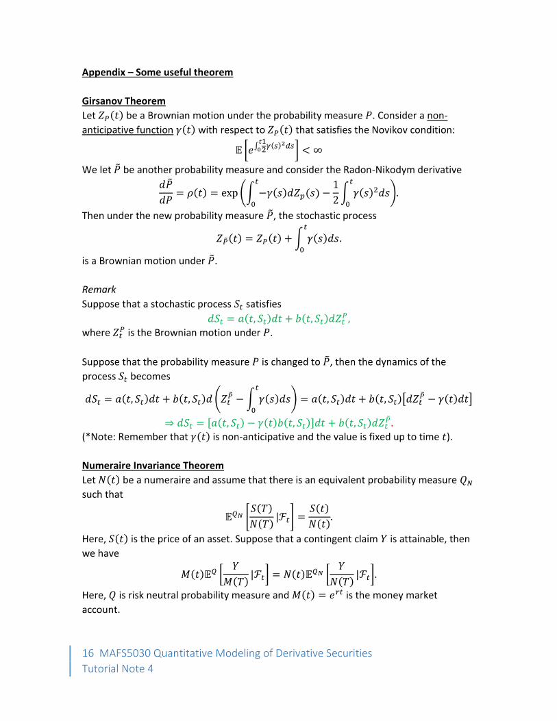
Appendix – Some useful theorem

Girsanov Theorem

Let 𝑍𝑃(𝑡) be a Brownian motion under the probability measure 𝑃. Consider a non-

anticipative function 𝛾(𝑡) with respect to 𝑍𝑃(𝑡) that satisfies the Novikov condition:

𝔼 [𝑒∫12𝛾(𝑠)2𝑑𝑠

𝑡0 ] < ∞

We let �̃� be another probability measure and consider the Radon-Nikodym derivative

𝑑�̃�

𝑑𝑃= 𝜌(𝑡) = exp(∫ −𝛾(𝑠)𝑑𝑍𝑝(𝑠)

𝑡

0

−1

2∫ 𝛾(𝑠)2𝑑𝑠𝑡

0

).

Then under the new probability measure �̃�, the stochastic process

𝑍�̃�(𝑡) = 𝑍𝑃(𝑡) + ∫ 𝛾(𝑠)𝑑𝑠𝑡

0

.

is a Brownian motion under �̃�.

Remark

Suppose that a stochastic process 𝑆𝑡 satisfies

𝑑𝑆𝑡 = 𝑎(𝑡, 𝑆𝑡)𝑑𝑡 + 𝑏(𝑡, 𝑆𝑡)𝑑𝑍𝑡𝑃,

where 𝑍𝑡𝑃 is the Brownian motion under 𝑃.

Suppose that the probability measure 𝑃 is changed to �̃�, then the dynamics of the

process 𝑆𝑡 becomes

𝑑𝑆𝑡 = 𝑎(𝑡, 𝑆𝑡)𝑑𝑡 + 𝑏(𝑡, 𝑆𝑡)𝑑 (𝑍𝑡�̃� −∫ 𝛾(𝑠)𝑑𝑠

𝑡

0

) = 𝑎(𝑡, 𝑆𝑡)𝑑𝑡 + 𝑏(𝑡, 𝑆𝑡)[𝑑𝑍𝑡�̃� − 𝛾(𝑡)𝑑𝑡]

⇒ 𝑑𝑆𝑡 = [𝑎(𝑡, 𝑆𝑡) − 𝛾(𝑡)𝑏(𝑡, 𝑆𝑡)]𝑑𝑡 + 𝑏(𝑡, 𝑆𝑡)𝑑𝑍𝑡�̃�.

(*Note: Remember that 𝛾(𝑡) is non-anticipative and the value is fixed up to time 𝑡).

Numeraire Invariance Theorem

Let 𝑁(𝑡) be a numeraire and assume that there is an equivalent probability measure 𝑄𝑁

such that

𝔼𝑄𝑁 [𝑆(𝑇)

𝑁(𝑇)|ℱ𝑡] =

𝑆(𝑡)

𝑁(𝑡).

Here, 𝑆(𝑡) is the price of an asset. Suppose that a contingent claim 𝑌 is attainable, then

we have

𝑀(𝑡)𝔼𝑄 [𝑌

𝑀(𝑇)|ℱ𝑡] = 𝑁(𝑡)𝔼

𝑄𝑁 [𝑌

𝑁(𝑇)|ℱ𝑡].

Here, 𝑄 is risk neutral probability measure and 𝑀(𝑡) = 𝑒𝑟𝑡 is the money market

account.

mafs5030 quantitative modeling of derivative securities

Documents