magnetic field feature analysis of smartphone application ...magnetic field feature analysis of...
TRANSCRIPT

University of California
Los Angeles
Magnetic Field Feature Analysis of Smartphone
Application Activities Using Android MI
Sensors
A project submitted in partial satisfaction
of the requirements for the degree
Master of Science in Electrical Engineering
by
Hsin-Hao Chiang
2013

c© Copyright by
Hsin-Hao Chiang
2013
Abstract of the Project
Magnetic Field Feature Analysis of Smartphone
Application Activities Using Android MI
Sensors
by
Hsin-Hao Chiang
Master of Science in Electrical Engineering
University of California, Los Angeles, 2013
Professor Mani Srivastava, Chair
In this project, the magnetic field data of three axes are read by the mag-
netometer in an Android Smartphone and are recorded by an application then
processed through MATLAB. Various denoising techniques and frequency domain
analysis is implemented and two sets of experiment are designed by varying the
direction, the phone activity, and the distance.
The first experiment is done in order to analyze the magnetic field feature
generated by another smartphone, whereas the second experiment is to monitor
the change of the magnetic field due to different activities running on the same
phone. WiFi transmitting and music-playing activities are chosen for the test, and
different characteristics of magnetic field features are discovered respectively.
ii

The project of Hsin-Hao Chiang is approved.
Co-chair 1 name
Co-chair 2 name
Co-chair 3 name
Mani Srivastava, Committee Chair
University of California, Los Angeles
2013
iii

Table of Contents
1 Introduction . . . . . . . . . . . . . . . . . . . . . . . . . . . . . . . . 1
1.1 Magnetometer . . . . . . . . . . . . . . . . . . . . . . . . . . . . . 1
1.2 Data Processing Method . . . . . . . . . . . . . . . . . . . . . . . 2
2 Experiment Result and Discussion . . . . . . . . . . . . . . . . . . 5
2.1 Experiment I . . . . . . . . . . . . . . . . . . . . . . . . . . . . . 5
2.1.1 Experiment Design . . . . . . . . . . . . . . . . . . . . . . 5
2.1.2 Experimental Result . . . . . . . . . . . . . . . . . . . . . 6
2.1.3 Discussion . . . . . . . . . . . . . . . . . . . . . . . . . . . 10
2.2 Experiment II . . . . . . . . . . . . . . . . . . . . . . . . . . . . . 11
2.2.1 Experiment Design . . . . . . . . . . . . . . . . . . . . . . 11
2.2.2 Experimental Result . . . . . . . . . . . . . . . . . . . . . 11
3 Conclusion . . . . . . . . . . . . . . . . . . . . . . . . . . . . . . . . . 13
3.1 Summary . . . . . . . . . . . . . . . . . . . . . . . . . . . . . . . 13
3.2 Future Work . . . . . . . . . . . . . . . . . . . . . . . . . . . . . . 14
References . . . . . . . . . . . . . . . . . . . . . . . . . . . . . . . . . . . 16
iv

List of Figures
1.1 Sample input data. . . . . . . . . . . . . . . . . . . . . . . . . . . 3
1.2 Denoised norm. . . . . . . . . . . . . . . . . . . . . . . . . . . . . 3
1.3 STFT output. . . . . . . . . . . . . . . . . . . . . . . . . . . . . . 4
1.4 Scatter plot. . . . . . . . . . . . . . . . . . . . . . . . . . . . . . . 4
2.1 Phone orientation. [2] . . . . . . . . . . . . . . . . . . . . . . . . . 5
2.2 +x, 0 ft. . . . . . . . . . . . . . . . . . . . . . . . . . . . . . . . . 6
2.3 +x, 0.5 ft. . . . . . . . . . . . . . . . . . . . . . . . . . . . . . . . 6
2.4 +x, 1.0 ft. . . . . . . . . . . . . . . . . . . . . . . . . . . . . . . . 7
2.5 +x, 1.5 ft. . . . . . . . . . . . . . . . . . . . . . . . . . . . . . . . 7
2.6 +y, 0 ft. . . . . . . . . . . . . . . . . . . . . . . . . . . . . . . . . 7
2.7 +y, 0.5 ft. . . . . . . . . . . . . . . . . . . . . . . . . . . . . . . . 7
2.8 +y, 1.0 ft. . . . . . . . . . . . . . . . . . . . . . . . . . . . . . . . 8
2.9 +y, 1.5 ft. . . . . . . . . . . . . . . . . . . . . . . . . . . . . . . . 8
2.10 +z, 0 ft. . . . . . . . . . . . . . . . . . . . . . . . . . . . . . . . . 8
2.11 +z, 0.5 ft. . . . . . . . . . . . . . . . . . . . . . . . . . . . . . . . 8
2.12 +z, 1.0 ft. . . . . . . . . . . . . . . . . . . . . . . . . . . . . . . . 9
2.13 +z, 1.5 ft. . . . . . . . . . . . . . . . . . . . . . . . . . . . . . . . 9
2.14 Experiment II. . . . . . . . . . . . . . . . . . . . . . . . . . . . . 12
2.15 Experiment II zoom in. . . . . . . . . . . . . . . . . . . . . . . . . 12
v

List of Tables
vi

CHAPTER 1
Introduction
1.1 Magnetometer
The numbers and accuracy of sensors in Android Smartphone has increased tremen-
dously since it has first been invented. Current Android API 17 indicates that
nowadays a typical smartphone usually comes with sensors including accelerome-
ter, gyroscope, proximity sensor, light sensor, and magnetometer, and some even
have temperature and humidity sensors[1]. Data from single or multiple sensors
provides information such as location, speed, orientation, or status of the phone or
the user, which can further been processed for application usage, such as location-
based services or gaming experience.
Among all the sensors, magnetometer has not widely been used or explored as a
major sensor. In other industry magnetometer is already been used, such as vehi-
cle detection[5]. Currently on Google Market most applications of magnetometer
are for compass, metal detector, or simply magnetic field recorder. However, there
are applications that use the magnetic data to achieve indoor navigation, such as
IndoorAtlas ltd[6]. A team in Microsoft also do the indoor proximity detection by
analyzing magnetic field characteristic, and they also claim that magnetometer
has sharper boundaries, more consistent over time, and more resistant to interfer-
ence than other techniques such as 802.15.4, Bluetooth Low Energy, or RFID in
proximity detection[8].
Apple Inc. recently has patented a new method for triggering network device
1

discovery using magnetometer[4]. The speaker of the smartphone is connected to a
magnetic field signature generator which generates a special pattern corresponding
to the distinct ID of the phone. After the phone detects the specific magnetic
feature, it then determines which type the object is and initiates the connection
using Bluetooth, WiFi, or other connection protocols. The benefit for this scheme
is lower energy consumption since magnetometer alone consumes less power than
WiFi communication, and a new connection can be searched in magnetic domain
while old connection remains active.
Since no phone has had the build-in magnetic feature generator yet, the pur-
pose of the experiment is to determine if a phone can be discovered easily by its
nature magnetic field, and what WiFi signals or speakers oscillation when music
is played would influence the magnetic field value.
The smartphone used in the experiment is LG P999/G2X[7], and its mag-
netometer is AMI304, manufactured by Aichi Steel[3]. It has three magneto-
impedance sensors aligned in 3 axes, and the sensitivity is 600 LSB/Gauss, or
0.167 uT.
Using the Android API SensorManager, one timestamp and three magnetic
field data is fetched in every event. The fastest sampling frequency can be achieved
by setting the delay to SENSOR DELAY FASTEST. The resulting actual
sampling frequency tested on the device is 30 Hz.
1.2 Data Processing Method
An Android application is written to record and calculation the magnetic value
of x, y, z, direction and the norm. The norm is calculated by the formula
Bn = 2
√B2
x + B2y + B2
z (1.1)
The data is recorded in a .csv file. Further analysis is done by MATLAB
2

scripts. The sample input file is shown in Figure 1.1. 60 seconds of input data
are recorded.
The norm value is then passed into a denoising filter using MATLAB script
cmddenoise(). The filter performs an interval-dependent denoising of the signal,
using a wavelet decomposition. Daubechies wavelet transform with level N = 8
is selected in this report, and the formula is shown in follow. Let
P (y) =N−1∑k=0
(n
k
)yk, where
(n
k
)denotes the binomial coefficients. (1.2)
Then
|m0(ω)|2 = ((cos2(ω
2))NP (sin2(
ω
2)), where m0(ω) =
1√2
2N−1∑k=0
hke−ikω (1.3)
The input and output of the filter is shown in Figure 1.2.
5770 5780 5790 5800 5810 5820 583040
60
80
100
120
140
160
180
t (sec)
ma
gn
etic f
ield
(u
T)
x
y
z
n
Figure 1.1: Sample input data.
200 400 600 800 1000 1200 1400 1600167
167.5
168
168.5
169
169.5
170
170.5
171
t (sec)
ma
gn
etic f
ield
(u
T)
Original
Denoised by db8
Figure 1.2: Denoised norm.
In order to analyze the frequency characteristics, Short-Time Fourier Trans-
form(STFT) is implemented on the denoised signal. Setting nfft = 32, noverlap
= 30, the output matrix is shown in Figure 1.3, and each column represents the
instant frequency distribution from 0 to 32 Hz for the short time interval.
The final step is to observe the low and high frequency characteristics. We
sum up the power ranging from 5 to 8 Hz to represent low frequency(X), and 15
3

5 10 15 20 25 30 35 40 45 500
5
10
15
t (sec)
f (H
z)
Figure 1.3: STFT output.
0.7 0.75 0.8 0.85 0.9 0.950
0.005
0.01
0.015
low freq power (5−8Hz)
hig
h f
req
po
we
r (1
5−
18
Hz)
Figure 1.4: Scatter plot.
to 18 Hz for high frequency(Y). Then for each short time interval, we obtain a
pair of power values (X,Y). By plotting Y vs X on a 2-D scatter plot, the pattern
of the specific condition can be observed (see Figure 1.4), and different status can
be further categorized.
4
CHAPTER 2
Experiment Result and Discussion
Two sets of experiments are done in this report. The first one is using an Android
smartphone (phone A) to monitor the magnetic field generated by another An-
droid smartphone (phone B). The second one is done using a single phone with
different application running and recording at the same time.
2.1 Experiment I
2.1.1 Experiment Design
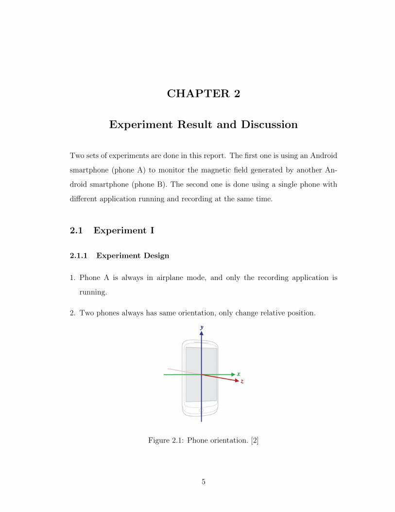
1. Phone A is always in airplane mode, and only the recording application is
running.
2. Two phones always has same orientation, only change relative position.
Figure 2.1: Phone orientation. [2]
5
3. The orientation of the phone is shown in Figure 2.1. Phone B is put in direction
+x, +y, or +z of phone A for testing.
4. Five different scenarios of phone B:
(a) not present
(b) airplane mode: idle
(c) WiFi active: transmitting WiFi packets
(d) music active: playing music in airplane mode
(e) WiFi and music active: transmitting packets and playing music at the
same time
5. Four different distances are tested: 0 ft, 0.5 ft, 1 ft, 1.5 ft.
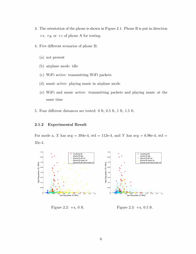
2.1.2 Experimental Result
For mode a, X has avg = 394e-4, std = 112e-4, and Y has avg = 6.96e-4, std =
35e-4.
0 0.02 0.04 0.06 0.08 0.1 0.12 0.14 0.16 0.18 0.20
0.005
0.01
0.015
0.02
0.025
0.03
0.035
0.04
low freq power (5−8Hz)
hig
h f
req
po
we
r (1
5−
18
Hz)
no phone B
phone B idle
phone B wifi on
phone B music on
phone B wifi and music on
Figure 2.2: +x, 0 ft.
0 0.02 0.04 0.06 0.08 0.1 0.12 0.14 0.16 0.18 0.20
0.005
0.01
0.015
0.02
0.025
0.03
0.035
0.04
low freq power (5−8Hz)
hig
h f
req
po
we
r (1
5−
18
Hz)
no phone B
phone B idle
phone B wifi on
phone B music on
phone B wifi and music on
Figure 2.3: +x, 0.5 ft.
6

0 0.02 0.04 0.06 0.08 0.1 0.12 0.14 0.16 0.18 0.20
0.005
0.01
0.015
0.02
0.025
0.03
0.035
0.04
low freq power (5−8Hz)
hig
h f
req
po
we
r (1
5−
18
Hz)
no phone B
phone B idle
phone B wifi on
phone B music on
phone B wifi and music on
Figure 2.4: +x, 1.0 ft.
0 0.02 0.04 0.06 0.08 0.1 0.12 0.14 0.16 0.18 0.20
0.005
0.01
0.015
0.02
0.025
0.03
0.035
0.04
low freq power (5−8Hz)
hig
h f
req
po
we
r (1
5−
18
Hz)
no phone B
phone B idle
phone B wifi on
phone B music on
phone B wifi and music on
Figure 2.5: +x, 1.5 ft.
Table 2.1: x direction (in 1E-4)
0 ft 0.5 ft
b c d e b c d e
xavg 349.76 167.00 692.69 339.73 334.45 267.43 504.11 340.84
xstd 92.82 24.91 205.45 296.12 153.33 100.86 87.12 225.79
yavg 2.03 0.36 6.52 4.63 2.05 1.70 1.52 5.07
ystd 10.78 1.78 30.96 19.18 8.12 9.32 9.98 14.50
1ft 1.5 ft
b c d e b c d e
xavg 484.34 260.92 674.37 287.17 340.34 244.99 449.60 318.92
xstd 133.92 79.97 6.31 77.90 113.59 46.80 41.85 158.47
yavg 1.78 0.60 0.44 6.79 1.20 2.42 0.53 8.31
ystd 7.88 1.93 0.01 25.70 3.96 10.25 1.28 40.09
0 0.02 0.04 0.06 0.08 0.1 0.12 0.14 0.16 0.18 0.20
0.005
0.01
0.015
0.02
0.025
0.03
0.035
0.04
low freq power (5−8Hz)
hig
h f
req
po
we
r (1
5−
18
Hz)
no phone B
phone B idle
phone B wifi on
phone B music on
phone B wifi and music on
Figure 2.6: +y, 0 ft.
0 0.02 0.04 0.06 0.08 0.1 0.12 0.14 0.16 0.18 0.20
0.005
0.01
0.015
0.02
0.025
0.03
0.035
0.04
low freq power (5−8Hz)
hig
h f
req
po
we
r (1
5−
18
Hz)
no phone B
phone B idle
phone B wifi on
phone B music on
phone B wifi and music on
Figure 2.7: +y, 0.5 ft.
7

0 0.02 0.04 0.06 0.08 0.1 0.12 0.14 0.16 0.18 0.20
0.005
0.01
0.015
0.02
0.025
0.03
0.035
0.04
low freq power (5−8Hz)
hig
h f
req
po
we
r (1
5−
18
Hz)
no phone B
phone B idle
phone B wifi on
phone B music on
phone B wifi and music on
Figure 2.8: +y, 1.0 ft.
0 0.02 0.04 0.06 0.08 0.1 0.12 0.14 0.16 0.18 0.20
0.005
0.01
0.015
0.02
0.025
0.03
0.035
0.04
low freq power (5−8Hz)
hig
h f
req
po
we
r (1
5−
18
Hz)
no phone B
phone B idle
phone B wifi on
phone B music on
phone B wifi and music on
Figure 2.9: +y, 1.5 ft.
Table 2.2: y direction (in 1E-4)
0 ft 0.5 ft
b c d e b c d e
xavg 394.36 810.28 570.69 935.73 362.88 868.53 526.93 880.30
xstd 135.26 20.51 17.03 41.21 196.48 17.05 7.89 81.17
yavg 8.12 0.83 0.38 2.36 10.17 0.61 0.36 3.22
ystd 32.52 1.57 0.05 11.93 45.64 0.15 0.04 17.15
1ft 1.5 ft
b c d e b c d e
xavg 537.22 854.87 530.02 840.45 793.89 835.46 476.56 864.15
xstd 60.64 23.93 7.54 44.00 27.22 30.02 19.31 61.03
yavg 0.88 0.60 0.36 0.74 1.21 0.56 0.33 0.60
ystd 2.12 0.08 0.02 1.15 4.03 0.05 0.04 0.09
0 0.05 0.1 0.15 0.2 0.25 0.3 0.35 0.40
0.005
0.01
0.015
0.02
0.025
0.03
0.035
0.04
low freq power (5−8Hz)
hig
h f
req
po
we
r (1
5−
18
Hz)
no phone B
phone B idle
phone B wifi on
phone B music on
phone B wifi and music on
Figure 2.10: +z, 0 ft.
0 0.05 0.1 0.15 0.2 0.25 0.3 0.35 0.40
0.005
0.01
0.015
0.02
0.025
0.03
0.035
0.04
low freq power (5−8Hz)
hig
h f
req
po
we
r (1
5−
18
Hz)
no phone B
phone B idle
phone B wifi on
phone B music on
phone B wifi and music on
Figure 2.11: +z, 0.5 ft.
8

0 0.05 0.1 0.15 0.2 0.25 0.3 0.35 0.40
0.005
0.01
0.015
0.02
0.025
0.03
0.035
0.04
low freq power (5−8Hz)
hig
h f
req
po
we
r (1
5−
18
Hz)
no phone B
phone B idle
phone B wifi on
phone B music on
phone B wifi and music on
Figure 2.12: +z, 1.0 ft.
0 0.05 0.1 0.15 0.2 0.25 0.3 0.35 0.40
0.005
0.01
0.015
0.02
0.025
0.03
0.035
0.04
low freq power (5−8Hz)
hig
h f
req
po
we
r (1
5−
18
Hz)
no phone B
phone B idle
phone B wifi on
phone B music on
phone B wifi and music on
Figure 2.13: +z, 1.5 ft.
Table 2.3: z direction (in 1E-4)
0 ft 0.5 ft
b c d e b c d e
xavg 202.22 561.60 451.79 418.50 460.11 2443.46 2232.22 2389.61
xstd 180.54 303.37 19.90 140.76 39.68 132.39 158.33 139.29
yavg 8.64 12.45 0.31 3.32 0.50 3.02 4.45 3.21
ystd 38.44 37.88 0.03 25.61 0.95 7.38 21.22 7.94
1ft 1.5 ft
b c d e b c d e
xavg 206.94 350.28 2173.10 374.39 302.67 339.17 2180.33 258.46
xstd 113.19 458.52 164.94 474.71 261.79 285.27 81.87 390.34
yavg 5.13 21.47 2.94 12.81 8.47 11.10 3.07 9.50
ystd 21.17 73.66 6.15 37.89 28.77 48.02 15.59 43.74
9

2.1.3 Discussion
1. In general
• When phone B is placed by phone A, Y is suppressed, ie. high frequency
power is lowered.
• The power does not decrease monotonically when the distance increases.
It is interesting that there exist some magnetic field peaks in some direc-
tion.
2. In terms of direction and distance:
• In direction +x, two phones are placed side by side, and therefore all
scenarios overlap each other and are not easy to be categorized. However,
it is still clear that mode (a) and mode (b) have similar X and in mode (c)
X remains in low power (around 0.02). Increase the distance only impacts
mode(d).
• In direction +y, mode (e) is most distinguished from others. Y in mode
(d) remains low and all Ys become zero when distance increases.
• In direction +z, phone B is on top of phone A, it has largest impact
to magnetic field when transmitting WiFi packets. However, the result
shows that the influence is not directly inverse relative to the distance.
mode (d) can barely observed when 0 ft, but can be observed in larger
distance, and its X even converge at 1.5 ft. It implies the magnetic field
of a smartphone has special pattern. Mode (c)(d)(e) all have larger X at
0.5 ft confirms this result.
3. In terms of scenario:
• In mode (a)(red cursor), phone A only records the weak magnetic field,
so Yis random and as large as 0.04 but X is stable within 0.03 and 0.05
10

• In mode (b)(green cursor), Yis lower than (a), and X is more concen-
trated. It is because phone B implies a small but constant magnetic field
on phone A, so the STFT result would be more static.
• In mode (c)(blue cursor), the WiFi module of phone B is constantly trans-
mitting packets and the magnetic is varying largely due to the change of
electromagnetic wave. Consequently, X and Y are both random.
• In mode (d)(yellow cursor), phone B plays a segment of music in airplane
mode, so the magnetic field is mostly influenced by the electromagnet in
the speaker. The resulting Yis relatively low (below 0.02), and X is static
around 0.05
• In mode (e)(cyan cursor), both WiFi transmission and music play are
active, As a result, the scatter plot is the superposition of mode (c) and
(d).
2.2 Experiment II
2.2.1 Experiment Design
The second experiment is done by monitoring the change of magnetic field when
the phone itself is running different activities. Similar activities are chosen: WiFi
packet transmission and music play. Phone call activity is also added.
2.2.2 Experimental Result
The scatter plot (Figure 2.14) shows that the phone call activity has large influence
on magnetic field compared to other activities. For other activities, the zoomed
plot (Figure 2.15) shows that it can easily detect its WiFi activity due to the
larger variance of X than idle, but music play is rather difficult to detect.
11

0 2 4 6 8 10 12 14 16 18 200
2
4
6
8
10
12
14
16
18
20
low freq power (5−8Hz)
hig
h fre
q p
ow
er
(15−
18H
z)
ariplane mode, idle
wifi mode, idle
wifi mode, transmitting packets
airplane mode, playing music
wifi mode, playing music
calling phone
Figure 2.14: Experiment II.
0 0.05 0.1 0.15 0.2 0.25 0.30
0.01
0.02
0.03
0.04
0.05
0.06
low freq power (5−8Hz)
hig
h fre
q p
ow
er
(15−
18H
z)
ariplane mode, idle
wifi mode, idle
wifi mode, transmitting packets
airplane mode, playing music
wifi mode, playing music
calling phone
Figure 2.15: Experiment II zoom in.
Table 2.4: Experiment II (in 1E-4)
a b c d e f
xavg 393.73 410.92 542.81 304.08 383.95 16360.75
xstd 111.83 83.99 517.58 154.60 335.48 27790.66
yavg 6.93 2.42 19.83 4.09 21.87 14677.55
ystd 35.24 13.56 69.50 25.32 116.32 24170.47
12

CHAPTER 3
Conclusion
3.1 Summary
1. The magnetic field characteristic of an Android smartphone varies significantly
depending on the status of the phone, the modules which are active, and the
applications which are running. Through frequency analysis using STFT, dif-
ferent status can be categorized statistically. The study implies that the mag-
netometer of the smartphone can be used not only as a compass, but more as a
detector or tracker of surrounding environment, or even the activities of itself.
2. Phone call generates large magnetic field and can be easily detected. It is
possibly due to the mobile network and depends on the signal strength. s
3. It is shown that the magnetic field would vary largely when WiFi packet trans-
mission is active. Further investigation could be done on differentiating differ-
ent type of WiFi activities, such as streaming video, file download, or social
networking update.
4. It is proved that playing music is proved to be affective the magnetic field.
Apple Inc. proposed the method to emit magnetic field spike using the speaker
should be feasible, but it should not generate unwanted sound at the same
time.
5. Different distances and phone orientations will result in different magnetic fea-
ture. An omni-directional detecting algorithm is needed in order to provide
13

more reliable categorization.
6. It could be a privacy issue since the magnetic field data can be easily captured
by third-party. It is interesting to study if any shielding can reduce such effect.
3.2 Future Work
1. The sampling period of the data provided by Android sensor API is not static,
and it depends on the priority of the application process and the loading of
the OS. In this report it is assumed that the sampling interval remains stable
in a short time period. The background running applications of the recording
smartphone is reduced to as few as possible, but sometimes jitter still happens.
It could be done by directly accessing the magnetometer data, but a general
user application should only use OS-provided API.
2. The change of DC or very low frequency value is not discussed in this report.
It is because sometimes significant changing of the magnetic field will cause
the magnetometer to become a very large value and lose track of actual DC
value. Only after the user moves or shakes the phone, it will recalibrate and
go back to the previous value. Apparently the large change of the magnetic
field indicates the change of the state, so if taking it into consideration, the
categorizing process may be more accurate.
3. Apple Inc. proposed a magnetic field signature generator coupled with the
speaker in order to generate the magnetic spike. It is interesting to study
which sound could generate such effect so that no additional hardware would
be needed.
4. The data is recorded and are processed off-line using MATALB. It can be done
by doing real-time calculation within the application on Android OS. However,
the computation loading may affect the sampling period as discussed in 1.
14

Multicore processors or carefully-designed software can be implemented
5. In Experiment II it is shown that the WiFi activity of itself will impact on the
detection of magnetometer. When a smartphone is in daily usage, i.e. mobile
network and WiFi active, the result can be anticipated to be more noisy and
harder to distinguish.
15

References
[1] Anrdoid API-Sensor. http://developer.android.com/reference/android/hardware/sensor.html.
[2] Android API-SensorEvent. http://developer.android.com/reference/android/hardware/sensorevent.html.
[3] Ami304 datasheet. http://www.aichi-mi.com/3 products/b9110329ami304e.pdf.
[4] Apple Inc. http://www.google.com/patents/us8290434.
[5] Yuqiao Shi Jinhui Lan. Vehicle detection and recognition based on a memsmagnetic sensor. IEEE International Conference on Nano/Micro Engineeredand Molecular Systems, January 2009.
[6] IndoorAtlas ltd. http://www.indooratlas.com/.
[7] G2X manual. http://extabit.com/file/28e6i5q276zn6/lg p999 p999dw t-mobile g2x service manual.rar.
[8] Kaifei Chen Ben Zhang Jeff Hsu Jie Liu Bin Cao Xiaofan Jiang, Chieh-JanMike Liang and Feng Zhao. Design and evaluation of a wireless magnetic-basedproximity detection platform for indoor applications. IPSN, April 2012.
16