magnetic field mapping of coiled current-carrying wires · magnetic field mapping of coiled...

WJP, PHY382 (2015) Wabash Journal of Physics v3.3, p.1

Magnetic Field Mapping of Coiled Current-Carrying Wires

A. Camacho, B. Hayhurst, K. Sullivan, and M. J. Madsen

Department of Physics, Wabash College, Crawfordsville, IN 47933

(Dated: March 17, 2015)

The purpose of this experiment is to create a three dimensional vector map of

the magnetic field of current-carrying coils of wire. We have measured the magnetic

field produced by a coiled, current-carrying wire at predetermined points around the

coil and superimposed each vector onto a plot to create a map of the magnetic field.

The ”maps” (plots) created by our apparatus agree very closely with the predicted

model. Future work on this experiment could include measuring the structure of the

magnetic field of a persistent current in a superconducting loop.


Magnetic field mapping can be used as a quality control assessment tool in production

of complex multipole magnets or complex assemblies such as loudspeakers or photocopier

rollers. By accurately knowing the behavior of a magnetic field, we can test the effectiveness

and efficiency of different ways to produce a magnetic field, [1] [2]. The purpose of this

experiment was to develop a method to accurately map out the magnetic field produced by

a coil with approximately constant current running through it [5].

I. MODEL

To Achieve the goal of our experiment, we have created a system for mapping the magnetic

field in three-dimensional space in a reliable and repeatable fashion. To do this we used

knowledge about how current-carrying wires and moving chargea produce magnetic fields.

Following from Jackson [5], we consider a circular loop of radius a, lying in the x − y

plane, centered at the origin, and carrying a constant current I. From Maxwell’s differential

laws of magnetostatics,

∇×B = µ0J (1)

and

∇ ·B = 0, (2)

we see that if ∇ · B = 0 everywhere, B must be the curl of some vector A(x), called the

vector potential,

B(x) = ∇×A(x). (3)

Thus, substituting Eq. (3) into Eq. (1) yields

∇× (∇×A) = µ0J (4)

or

∇(∇ ·A)−∇2A = µ0J. (5)

By making use of the Coulomb gauge, ∇ ·A = 0, equation 5 reduces to Poisson’s equation

∇2A = µ0J, (6)


and the general solution for A has the familiar form

A(x) =µ0

4π

∫J‘

|x− x‘|d3x‘. (7)

The current density J has only a component in the φ direction, thus

Jφ = I sin θ‘δ(cosθ‘)δ(r‘ − a)

a. (8)

The delta function restricts the current flow to a ring of radius a. Because of the symmetry

of our loop configuration, the x component of the current has no effect on the total magnetic

field. This leaves only a y component, which is Aφ

Aφ(r, θ) =µ0 I a

4π

∫ 2π

0

cosφ‘dφ‘

(a2 + r2 + 2arsinθcosφ‘)1/2. (9)

At this point we switched from Jackson’s use of spherical polar coordinates to cylindrical

polar coordinates. The reason behind this is that our solenoid could be modeled after a

cylnder and not a sphere. Our new formula for Aφ is then

Aφ(r, θ) =µ0 I a

4π

∫ π

−π

cosφ‘dφ‘

(a2 + s2 + z2 − 2ascosφ‘)1/2. (10)

The above integral expressed in terms of the complete elliptic integrals is

Aφ(r, θ) = −µ0 I

2πs

[(a+ s)2 + z2E(k)− (a2 + s2 + z2)K(k)]√(a+ s)2 + z2

, (11)

where

k =4 a s

(a+ s)2 + z2. (12)

Eq. (11) along with Eq. (12) is the vector potential for a single loop of wire. Along with

this, the components of magnetic induction in cylindrical coordinates are

Bs = −∂Aφ∂z

(13)

Bz =1

s

∂

∂s(sAφ) (14)

Bφ = 0. (15)

All we need to do now is add up all the loops that make up our solenoid while offseting the

z-position of the coils accordingly

Atotφ =

92∑

i=− 92

−µ0 I

2πs

[(a+ s)2 + (z − zi)2E(k)− (a2 + s2 + (z − zi)2)K(k)]√(a+ s)2 + (z − zi)2

(16)


with

k =4 a s

(a+ s)2 + (z − zi)2. (17)

Btots is then obtained by substituting the result of Eq. (16) into Eq. (13), and similarly,

Btotz is obtained by substituting the result of Eq. (16) into Eq. (14). The model for our

toilet-seat coil followed a similar method, with the exception that 5 turns of the coil were in

one direction while the other 5 turns were oriented in the opposite direction.

Z

Y

X

coil

magnometer#

FIG. 1: The above figure shows a simplified schematic of our setup. The magnetometer is

mounted on the end of a Lego wand that can actuate in each of the three directions shown.

A 10 turn coil of wire connected to a constant current power supply provides the model

magnetic field for the sensor to map. The magnetometer outputs data to the arduino

where the data is then processed and passed into a computer running National

Instruments LabView where the data is collected for further analysis.


II. SET UP

In an effort to repeat measurements with a good degree of reliability, we engineered an

automated mobile sensor support structure. The support structure moves in three dimen-

sions between predetermined points and is automated using programs coded using National

Instruments LabView that control Lego Mindstorms servo motors. This entire aparatus

moves a Honeywell Magnetometer between positions which gives the magnetic field vector

as a function of positon. This measurement allows us to create a map of the field. This

setup also allows for a reliable and repeatable measurement technique that also has a very

acceptable amount of accuracy.

In order to measure a magnetic field, we placed a Honeywell HMC5883L 3-Axis Mag-

netometer into the magnetic field using a 3-axis automated control mechanism. The data

collected from the sensor at each predetermined point gives the magnitude and direction of

the magnetic field at that point. Using a collection of points inside of the magnetic field

yields field map of the magnetic field.

To mitigate the effects of outside/background magnetic fields, we built the support struc-

ture and test bed from non-magnetic materials. The Legos, being plastic, and the aluminum

frame and test bed allow for the sensor to measure only the magnetic field caused by the

coil (a method for canceling out the Earths magnetic field is used but is described elsewhere

in this paper).

III. DATA ANALYSIS

The Honeywell magnetometer collects a magnitude of electric field in the x, y, and z

directions; To ensure the data collected from the magnetometer correlated to our theories,

we compared the theoretical model field map to the data collected by the magnetometer.

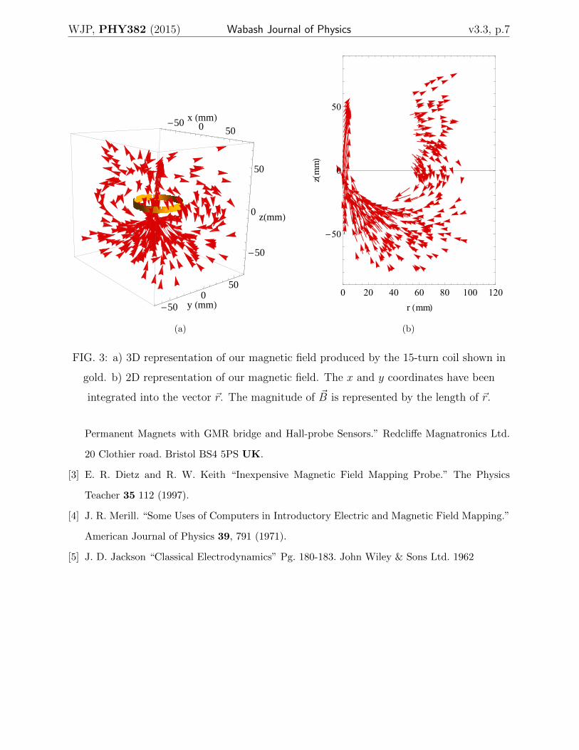
To plot the field and compare the fields, we plotted the magnetic field vector vs the position

of the sensor. As we can see from Figure 3, the map created by the apparatus is in strong

agreement with the predicted field. We can say, then, that the apparatus is a good tool for

measuring and mapping magnetic fields. Further calibration could increase the accuracy of

the apparatus, but as it is now, the apparatus works in a reliable fashion. This same sort of

comparison was done for multiple types of fields in an effort to ensure that the known fields


èè

èè

èè

èè

èè

èè

èè

èè

èè

èè

èè

èè

èè

èèè

èè

èè

èè

èè

èè

èè

èè

èè

èè

èè

èè

èè

èè

è

è DataFit

0 200 400 600 800 1000 1200 14000

50

100

150

raw position

yHm

mL

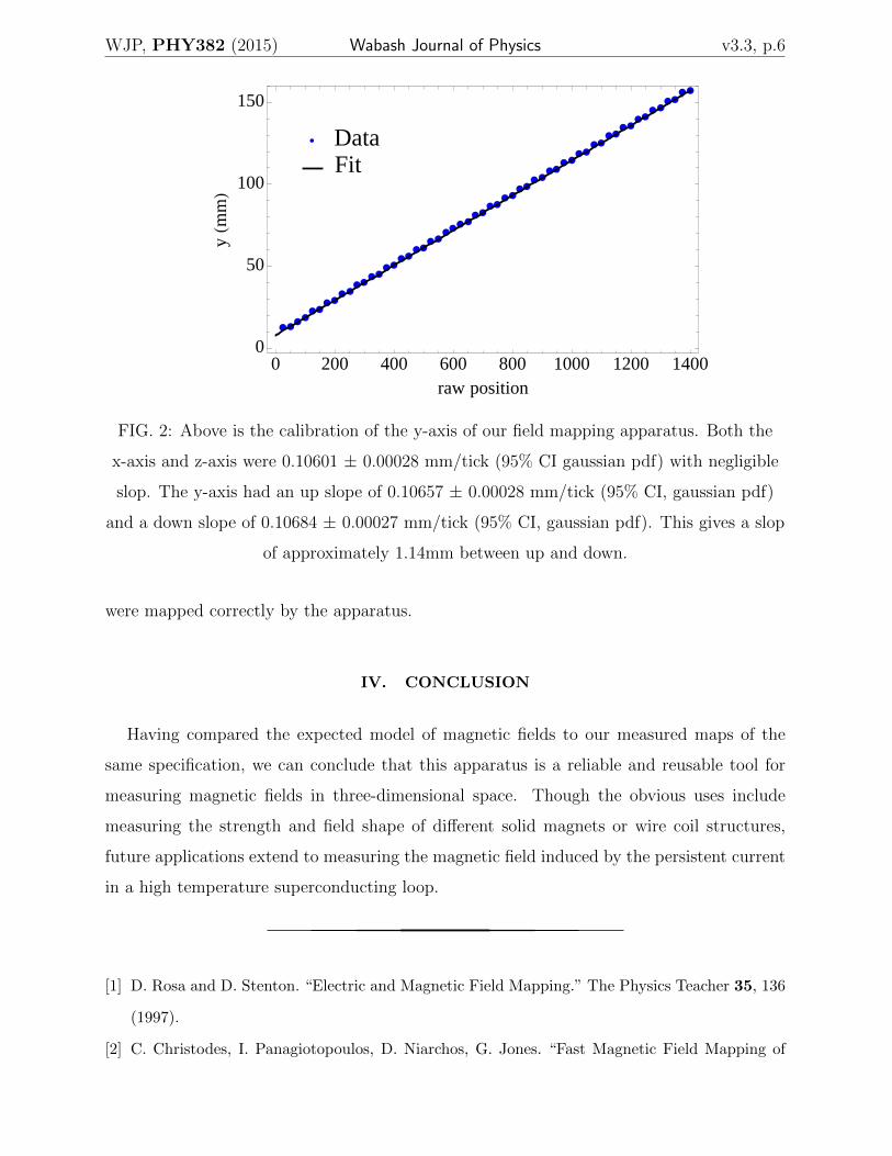
FIG. 2: Above is the calibration of the y-axis of our field mapping apparatus. Both the

x-axis and z-axis were 0.10601 ± 0.00028 mm/tick (95% CI gaussian pdf) with negligible

slop. The y-axis had an up slope of 0.10657 ± 0.00028 mm/tick (95% CI, gaussian pdf)

and a down slope of 0.10684 ± 0.00027 mm/tick (95% CI, gaussian pdf). This gives a slop

of approximately 1.14mm between up and down.

were mapped correctly by the apparatus.

IV. CONCLUSION

Having compared the expected model of magnetic fields to our measured maps of the

same specification, we can conclude that this apparatus is a reliable and reusable tool for

measuring magnetic fields in three-dimensional space. Though the obvious uses include

measuring the strength and field shape of different solid magnets or wire coil structures,

future applications extend to measuring the magnetic field induced by the persistent current

in a high temperature superconducting loop.

[1] D. Rosa and D. Stenton. “Electric and Magnetic Field Mapping.” The Physics Teacher 35, 136

(1997).

[2] C. Christodes, I. Panagiotopoulos, D. Niarchos, G. Jones. “Fast Magnetic Field Mapping of


-50 0 50

x HmmL

-50

050

y HmmL

-50

0

50

zHmmL

(a)

0 20 40 60 80 100 120

-50

0

50

r HmmLzHm

mL

(b)

FIG. 3: a) 3D representation of our magnetic field produced by the 15-turn coil shown in

gold. b) 2D representation of our magnetic field. The x and y coordinates have been

integrated into the vector ~r. The magnitude of ~B is represented by the length of ~r.

Permanent Magnets with GMR bridge and Hall-probe Sensors.” Redcliffe Magnatronics Ltd.

20 Clothier road. Bristol BS4 5PS UK.

[3] E. R. Dietz and R. W. Keith “Inexpensive Magnetic Field Mapping Probe.” The Physics

Teacher 35 112 (1997).

[4] J. R. Merill. “Some Uses of Computers in Introductory Electric and Magnetic Field Mapping.”

American Journal of Physics 39, 791 (1971).

[5] J. D. Jackson “Classical Electrodynamics” Pg. 180-183. John Wiley & Sons Ltd. 1962


0 20 40 60 80 100

-50

0

50

r HmmL

zHmm

L

(a)

0 20 40 60 80 100

-50

0

50

r HmmL

zHmm

L

(b)

FIG. 4: a) shows our data, as vectors, superimposed with our model as field lines for our

15 turn coil. The black rectangle is our source or coil b) The above figure shows our data,

as vectors, superimposed with our model as field lines for our toilet seat coil. The black

rectangle is our source or coil.


àà

à

à

à

à

à

à

à

à

à

àà

à

à

à

à

à

à

à

à

à

à

à

àà

ææ

ææ

æ

æ

æ

æ ææ

æ

æ

æ

æ

æ

æ ææ

æ

ææ

ææ

ææ

æ

UC Model

à UC Data

TS Model

æ TS Data

-40 -20 0 20 40

500.

1000.

1500.

2000.

2500.

-255

-127

0

127

255

z HmmL

Bz

HmG

L

FIG. 5: The above figure shows and overlay of the magnetic field data and model for a

z-axis scan through the center of the coils.

magnetic field mapping of coiled current-carrying wires · magnetic field mapping of coiled...

Documents