magnetic moment definitions of field quantities and

Characterization of Materials, edited by Elton N. Kaufmann.Copyright � 2012 John Wiley & Sons, Inc.

MAGNETIC MOMENTAND MAGNETIZATION

MICHAEL E. MCHENRY AND DAVID E. LAUGHLIN

Carnegie Mellon University, Pittsburgh, PA, USA

INTRODUCTION

Magnetismhas engaged explorers and scientists for overtwo millennia. The ancient Greeks and Turks notedthe attraction between magnetite (lodestone) and iron(Cullity and Graham, 1978). Explorers used lodestone’smagnetization to construct compass needles used topoint to the direction of the earth’s magnetic NorthPole. This singularly important device aided in naviga-tion and the exploration of the planet. Today, theminiaturization of magnetic sensors has propelled themagnetic recording industry as well as contributed tofar-reaching applications such as planetary exploration(Diaz-Michelena, 2009).

Michael Faraday’s (1791–1867) discovery of electro-magnetic inductionprovides theprinciple forunderstand-ing theoperationofelectric generators, transformers,anda variety of other magnetic devices. The quantummechanical description of the origin of atomic magneticdipole moments provides the basis for understanding avariety of disparate phenomena including the magneticresponse of materials.

The intrinsicmagnetic properties ofmaterials refer to:

i. the origin, magnitude, and directions of atomicmagnetic dipole moments;

ii. the nature of the interaction between atomicmagnetic dipole moments on neighboring atomsin the solid;

iii. whether these result in collective magnetic phe-nomena; and

iv. the resulting temperature dependence of themagnetization.

For materials exhibiting collective magnetic response,otherintrinsicmagneticpropertiesincludethestrengthofthe coupling of magnetic moments to one another andto crystallographic directions, magnetoelastic couplingcoefficients, and the temperature(s) at which magneticphase transformations occur. The intrinsic magneticproperties, of species at surfaces and interfaces, areknown to be distinctly different from those of the bulkinmany cases. This article reviews the theory of intrinsicmagneticpropertiesofdipolemomentandmagnetizationas well as theory and examples of collective magneticresponse. The National Institute of Standards and Tech-nology (NIST) keeps an up-to-date compilation of units.ThesecanbefoundinR.B.GoldfarbandF.R.Fickett,U.S.DepartmentofCommerce,NationalBureauofStandards,Boulder, Colorado80303,March1985NBSSpecial Pub-lication696forsalebytheSuperintendentofDocuments,U.S.GovernmentPrintingOffice,Washington,DC20402.

DEFINITIONS OF FIELD QUANTITIES

Discussion of the magnetic properties of materialsbegins by defining macroscopic field quantities.1 Thetwo fundamental quantities are the magnetic induction,~B, and the magnetic field, ~H , both of which are axialvector quantities. In many cases the induction and thefield will be collinear (parallel) so that we can treat themas scalar quantities, B and H.2

In a vacuum, the magnetic induction, ~B, is related tothe magnetic field, ~H :

~B ¼ m0 ~H ; ~B ¼ ~H ð1Þ

where the permeability of the vacuum, m0, is4p� 10�7 H=m in SI (mksa) units. This quantity is takenas 1 in cgs units. In cgs units, the induction and fieldhave the same values. In SI (mksa) units we assign apermeability to the vacuum, so the two are proportional.

In a magnetic material the magnetic induction canbe enhanced or reducedby thematerial’smagnetization,~M (defined as net dipole moment per unit volume),so that

~B ¼ m0ð~H þ ~M Þ; ~B ¼ ~H þ4p~M ð2Þ

where the magnetization, ~M , is expressed in linearresponse theory as

~M ¼ wm ~H ð3Þ

and the constant of proportionality is called themagneticsusceptibility, wm. The magnetic susceptibility thatrelates two vector quantities is a polar second-ranktensor. For most discussions (whenever B and H arecollinear or when interested in the magnetization com-ponent in the field direction) we treat the susceptibilityas a scalar.

Wecontinueourdiscussionconsidering scalar induc-tion, field, and magnetization. We can further expressB ¼ mrH as

B ¼ m0ð1þ wmÞH ; B ¼ ð1þ4pwmÞH ð4Þ

and we see that the relative permeability, mr, can beexpressed as

mr ¼ m0ð1þ wmÞ; mr ¼ 1þ4pwm ð5Þ

mr thus represents an enhancement factor of the fluxdensity in a magnetic material due to the magnetizationthat is an intrinsic material property. If we have wm < 0,we speak of diamagnetic response, and for wm > 0 (andno collective magnetism) we speak of paramagnetic

1 Selected formulas are introduced in SI (mksa) units followedby cgs units.2 Formany discussions it is sufficient to treat field quantities asscalars; when this is not the case, vector symbols will be explic-itly used.

response. A superconductor is a material that acts as a

perfect diamagnet so that wm ¼ �1 or wm ¼ �1

4p.

MAGNETIC DIPOLE MOMENTS—DEFINITIONSAND ATOMIC ORIGINS

A magnetic dipole moment has its origin in circulatingcharge (Fig. 1). This concept is made more complicatedby the need to treat circulating charges of electronswithin the framework of quantum mechanics.

Concepts relating circulating charge, angularmomentum, and dipole moments are:

i. A dipole moment for a circulating charge isdefined formally as

~m ¼ IA~u~r�~J ¼ðV

~r � ~J dV ð6Þ

where ~r is the position vector of the charged particleabout the origin for the rotation. ~r is the currentdensity of the orbiting charge. I is the current dueto the circulating charge,A ¼ pr2 is the area swept outby the circulating charge, andV is the volume. ~u~r�~J isa unit vector normal to the area, A.

ii. We relate the magnetic dipole moment to theangular momentum. Let ~P be a general angularmomentum vector. In classical mechanics, theangular momentum vector, expressed as~P ¼ ~r �m~v, hasmagnitudemvr ¼ mo0r

2, whereo0 is an angular frequency, and is directed nor-mal to the current loop (parallel to the dipolemoment). The fundamental relationship betweenmagnetic dipole moment and the angularmomentum vector is

m ¼ ge

2mP; m ¼ g

e

2mcP ð7Þ

where g is called the Lande g-factor. For an orbitingelectron the constant g ¼ 1. The dipole momentassociated with spin angular momentum has g ¼ 2.

iii. In quantum mechanics, every electron has adipole moment associated with its spinningcharge density (spin) and its orbit about thenucleus (orbit). Angular momentum (whetherspin or orbital) is quantized in units of Planck’s

constant divided by 2p, that is, �h ¼ h

2p¼ 1:05�

10�34 J s ¼ 1:05� 10�27 erg s.Wedefine the fun-damental unit of magnetic dipole moment, theBohr magneton, as

mB ¼ e

2m�h; m ¼ mB ¼ e

2mc�h ð8Þ

The Bohr magneton is calculated to have thefollowing value:

mB ¼ 9:27� 10�24 Am2 ðJ=TÞ;

m ¼ mB ¼ 9:27� 10�21 erg=G ð9Þ

iv. An atomic dipole moment is calculated by sum-mingall of the electrondipolemoments for a givenatomic species. Quantum mechanical rules forthis summing called Hund’s rules are discussedbelow.

v. For a collection of identical atoms the magneti-zation, M, is

M ¼ Namatom ð10Þ

where Na is the number of dipole moments per unitvolume and matom is the atomic dipole moment.

vi. The potential energy of a dipole moment in thepresence of a field is

Ep ¼~m � ~B ¼ mB cosy ð11Þ

where y is the angle between the dipole moment and~B. This implies that magnetization (or other fieldquantity) multiplied by another field has units ofenergy per unit volume. It is important to begin tothink of energy densities (energy per unit volume) formagnetic systems. In quantum mechanical systems,the component of the dipole moment vector projectedalong the field direction is quantized and only partic-ular values of the angle y are allowed.

Closed Shell Diamagnetism: Langevin Theoryof Diamagnetism

The diamagnetic susceptibility of closed shells is dis-cussed in Box 1.

Diamagnetism is the atomic magnetic response dueto closed shell orbits of core electrons.

This is tobe contrastedwith theperfectdiamagnetismof a superconductor. Magnetic flux is excluded from theinterior of a superconductor and it is a consequence of

B ¼ 0, which requires that wm ¼ �1 or wm ¼ �1

4p.

q v

r

μ

Figure 1. Geometryof a chargedparticle orbitingat adistance r,with a linear velocity, v. The particle orbit sweeps out anarea,A,and gives rise to a dipole moment, ~m.

2 MAGNETIC MOMENT AND MAGNETIZATION

The magnitude, L ¼ j~L j, of the orbital angularmomentum vector, ~L , and its projection, Lz, onto an axisof quantization, z, by the application of a field, Bz, isquantized in units of �h. For Lz the quantum number ml

quantizes theprojectedorbital angularmomentum.Thishas the further consequence that the orbital angularmomentum vector, ~L , can precess about the field axis,z, only at a set of discrete angles, y:

Lz ¼ ml�h; ml ¼ �l � � � 0 � � � þ l;

y ¼ arccosLz

L¼ arccos

ml

lð13Þ

Open Shell Atomic Dipole Moments—Hund’s Rules

We now examine systems where the electrons responsi-ble for the dipoles exist in localized states assigned to aparticular atom. In systems (typically ionic) where theatomic orbitals responsible for the magnetic dipolemoments are localized on specific atoms in a solid,discrete magnetic states can be calculated using quan-tummechanical rules calledHund’s rules (Hund, 1927).This discussion is applicable in understanding themag-netic dipoles in ionic systems such as oxides and salts oftransition metals.

A general angular momentum vector, ~P, can havecontributions from orbital angular momentum, ~L , andspin angular momentum, ~S . Both moments are quan-tized inunits of �h. The fundamental atomic unit of dipolemoment is the Bohr magneton.

In addition to the orbital moment, there is an addi-tional contribution to the magnetic moment of an elec-tron, due to spin. Spin is a purely quantum mechanicalproperty though we can view it semiclassically consid-ering an electron as a particle with a rotating surfacecurrent. The classical problem yields a spin momentsimilar to that which is derived in the quantummechan-ical description (Cullity and Graham, 1978).

Determining atomic dipole moments requires sum-ming spin and orbital angular momenta over all elec-trons on an atom. The summed orbital and spin angularmomenta is zero for closed shells. The closed shells thenonly contribute to the small diamagnetic moment of theprevious section.3 In open shells we need to considerrules for summing thespinandorbital angularmomentafor all electrons in the open shell. Hund’s rules allow usto describe the ground-state multiplet including the ml

and ms eigenstates and allow us to calculate the com-ponents of the orbital, L, spin, S, and total angular, J,momenta. The magnitudes of orbital and spin angularmomenta are constructed by summing angularmomen-tum over a multielectron shell:

L ¼Xni¼1

ðmlÞi�h; S ¼Xni¼1

2ðmsÞi�h ð14Þ

The projection of the total angular momentum vector,~J ¼ ~L þ ~S , along the applied field direction is alsosubject to quantization conditions. Hund’s rules requirethat J (J ¼ L þS) is jL�Sj for less than half-filledshells and jL þSj for greater than half-filled shells. Todetermine the occupation of eigenstates of S, L, and

MAGNETIC SUSCEPTIBILITY OF A SIMPLE DIAMAGNET

Consider an atom with a closed electronic shell. Forfilled shells, electrons orbit the nuclei, but the netcurrent associated with their motion is zero becauseof cancellation of their summed orbital angularmomentum, ~L (i.e., ~L ¼ 0). However, even for a closedshell, in the presence of an applied field a net currentis induced. By Lenz’s law this current results in adipole moment that opposes the applied field. TheLarmor frequency, oL, is the characteristic frequencyof this circulating induced current and has a value

oL ¼ eH

m; oL ¼ eH

mcð12aÞ

If we wish to construct an atomic dipole moment, wemust consider the moment due to Z electrons thatorbit the nucleus. Assuming that all Z electrons orbitthe nucleus with the same angular frequency, oL, weexpress the current, I, as follows:

I ¼ dq

dt¼ ZeoL

2pð12bÞ

The induced moment is calculated as the currentmultiplied by the area and the orbital atomic mag-netic dipole moment is then

matom ¼ �ZeoL

2

hr2i3

ð12cÞ

where the minus sign reflects Lenz’s law and hr2i isthe average value of r2 for the orbit. The average valueof the square of the orbital radius is

hr2i ¼ hx2iþ hy2iþ hz2i ð12dÞ

and for an isotropic environment:

hx2i ¼ hy2i ¼ hz2i ¼ hr2i3

ð12eÞ

Thismaybeassociatedwith thenegative diamagneticsusceptibility (for N atoms/volume):

wm ¼ NmatomH

¼ �NZe2

6m; wm ¼ Nmatom

H¼ �NZe2

6mc

ð12fÞ

which describes well the diamagnetism of coreelectrons and of closed shell systems. Typicallymolardiamagnetic susceptibilities are on the order of wm ¼10�6 to 10�5 cm3=mol ¼ 10�12 to 10�11 m3=mol.

3 For open shells this diamagnetic contribution is small enoughto ignore.

MAGNETIC MOMENT AND MAGNETIZATION 3

J we use Hund’s rules that state that for a closedelectronic shell J ¼ L ¼ S ¼ 0. For an open shell multi-electron atom:

i. We fill ml states (which are (2l þ1)-fold degener-ate) in such a way as to first maximize total spin.

ii. We fill ml states first in such a way as to firstmaximize total spin.

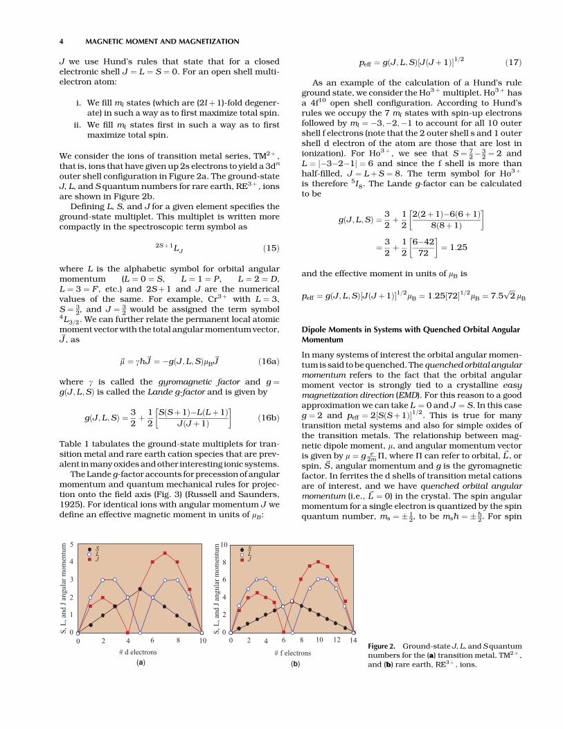
We consider the ions of transition metal series, TM2þ ,that is, ions that have given up 2s electrons to yield a 3dn

outer shell configuration in Figure 2a. The ground-stateJ, L, and S quantum numbers for rare earth, RE3þ , ionsare shown in Figure 2b.

Defining L, S, and J for a given element specifies theground-state multiplet. This multiplet is written morecompactly in the spectroscopic term symbol as

2Sþ1LJ ð15Þ

where L is the alphabetic symbol for orbital angularmomentum (L ¼ 0 ¼ S, L ¼ 1 ¼ P, L ¼ 2 ¼ D,L ¼ 3 ¼ F , etc.) and 2Sþ1 and J are the numericalvalues of the same. For example, Cr3þ with L ¼ 3,S ¼ 3

2, and J ¼ 32 would be assigned the term symbol

4L3=2. We can further relate the permanent local atomicmoment vectorwith the total angularmomentumvector,~J , as

~m ¼ g�h~J ¼ �gðJ ;L;SÞmB~J ð16aÞ

where g is called the gyromagnetic factor and g ¼gðJ ;L ;SÞ is called the Lande g-factor and is given by

gðJ ;L;SÞ ¼ 3

2þ 1

2

SðSþ1Þ�LðL þ1ÞJðJ þ1Þ

� �ð16bÞ

Table 1 tabulates the ground-state multiplets for tran-sition metal and rare earth cation species that are prev-alent inmanyoxidesandother interesting ionic systems.

TheLande g-factor accounts for precession of angularmomentum and quantum mechanical rules for projec-tion onto the field axis (Fig. 3) (Russell and Saunders,1925). For identical ions with angular momentum J wedefine an effective magnetic moment in units of mB:

peff ¼ gðJ ;L;SÞ½JðJ þ1Þ�1=2 ð17Þ

As an example of the calculation of a Hund’s ruleground state, we consider the Ho3þ multiplet. Ho3þ hasa 4f10 open shell configuration. According to Hund’srules we occupy the 7 ml states with spin-up electronsfollowed by ml ¼ �3;�2;�1 to account for all 10 outershell f electrons (note that the 2 outer shell s and 1 outershell d electron of the atom are those that are lost inionization). For Ho3þ , we see that S ¼ 7

2� 32 ¼ 2 and

L ¼ j�3�2�1j ¼ 6 and since the f shell is more thanhalf-filled, J ¼ L þS ¼ 8. The term symbol for Ho3þ

is therefore 5I8. The Lande g-factor can be calculatedto be

gðJ ;L;SÞ ¼ 3

2þ 1

2

2ð2þ1Þ�6ð6þ1Þ8ð8þ1Þ

� �

¼ 3

2þ 1

2

6�42

72

� �¼ 1:25

and the effective moment in units of mB is

peff ¼ gðJ ;L;SÞ½JðJ þ1Þ�1=2mB ¼ 1:25½72�1=2mB ¼ 7:5ffiffiffi2

pmB

Dipole Moments in Systems with Quenched Orbital AngularMomentum

In many systems of interest the orbital angular momen-tum is said tobequenched.Thequenchedorbital angularmomentum refers to the fact that the orbital angularmoment vector is strongly tied to a crystalline easymagnetization direction (EMD). For this reason to a goodapproximation we can take L ¼ 0 and J ¼ S. In this caseg ¼ 2 and peff ¼ 2½SðSþ1Þ�1=2. This is true for manytransition metal systems and also for simple oxides ofthe transition metals. The relationship between mag-netic dipole moment, m, and angular momentum vectoris given by m ¼ g e

2m P, where P can refer to orbital, ~L , orspin, ~S , angular momentum and g is the gyromagneticfactor. In ferrites the d shells of transition metal cationsare of interest, and we have quenched orbital angularmomentum (i.e., ~L ¼ 0) in the crystal. The spin angularmomentum for a single electron is quantized by the spinquantum number, ms ¼ � 1

2, to be ms�h ¼ � �h2. For spin

S, L

, and

J an

gula

r mom

entu

m

S, L

, and

J an

gula

r mom

entu

m

# f electrons# d electrons

0 00 02 2

2

1 2

4

3

4

5

4

4

6 6

6

8

8

8

10

10 1210 14

(a) (b)

SLJ

SLJ

Figure 2. Ground-state J, L, and S quantumnumbers for the (a) transition metal, TM2þ ,and (b) rare earth, RE3þ , ions.


only, the gyromagnetic factor is g ¼ 2, and the singleelectron dipole moment is

m ¼ �ge

2m

�h

2¼ � �he

2m; � g

e

2mc

�h

2¼ �he

2mcð18aÞ

m ¼ �ge

2m

�h

2or � g

e

2mc

�h

2ð18bÞ

Thus, m ¼ �mB with

mB ¼ 9:27� 10�24 Am2 ðJ=TÞ or 9:27� 10�21 erg=G

ð18cÞ

For a multielectron atom, the total spin angularmomentum is

S ¼Xni¼1

ðmsÞi�h

with the sum over electrons in the outer shell. Hund’srules determine the occupation of eigenstates of S.The first states that for an open shell multielectron atomwe fill the (2l þ1)-fold degenerate (for d electrons l ¼ 2,ð2l þ1Þ ¼ 5) orbital angular momentum states so as tomaximize total spin. To do so, wemust fill each of the fived states with a positive (spin-up) spin before returningto fill the negative (spin-down) spin. The total spin angu-lar momentum for 3d transition metal ions is summa-rized in Table 2. The dipole moments are all integralnumbers of Bohr magnetons allowing for simplificationof the analysis of the magnetization of ferrites that typ-ically have quenched angular momentum.

Atomic Dipole Moments—Energy Band Theory

In systemswith significant atomic overlap of the electronwave functions for orbitals responsible for magneticdipole moments, the energy and angular momentum

Table 1. Ground-State Multiplets of Common TM and RE Ions (Van Vleck, 1932)

Ion S L J

neff

Term g½JðJ þ1Þ�1=2 Observed g½SðSþ1Þ�1=2

d-Shell electrons1 Ti3þ , V4þ 1

2 2 32

2D3=2 1.55 1.70 1.732 V3þ 1 3 2 3F2 1.63 2.61 2.833 V2þ , Cr3þ 3

2 3 32

4F3=2 0.77 3.85 3.874 Cr2þ , Mn3þ 2 2 0 5D0 0 4.82 4.905 Mn3þ , Mn3þ 3

2 0 52

5S5=2 5.92 5.82 5.926 Fe2þ 2 2 4 5D4 6.7 5.36 4.907 Co2þ 3

2 3 92

4F9=2 6.63 4.90 3.878 Ni2þ 1 3 4 3F4 5.59 3.12 2.839 Cu2þ 1

2 2 52

2D5=2 3.55 1.83 1.7310 Cuþ , Zn2þ 0 0 0 1S0 0 0 0f-Shell electrons1 Ce3þ 1

2 3 52

2F5=2 2.54 2.512 Pr3þ 1 5 4 3H4 3.58 3.563 Nd3þ 3

2 6 92

4I9=2 3.62 3.34 Pm3þ 2 6 4 5I4 2.68 —5 Sm3þ 5

2 5 52

6H5=2 0.85 (1.6) 1.746 Eu3þ 3 3 0 7F0 0 (3.4) 3.47 Gd3þ , Eu3þ 5

2 0 52

8S7=2 7.94 7.988 Tb3þ 3 3 6 7F6 9.72 9.779 Dy3þ 5

2 5 152

6H15=2 10.63 10.6310 Ho3þ 2 6 8 5I8 10.60 10.411 Er3þ 3

2 6 152

4I15=2 9.59 9.512 Tm3þ 1 5 6 3H6 7.57 7.6113 Yb3þ 1

2 3 72

2F7=2 4.53 4.514 Lu3þ , Yb3þ 0 0 0 1S0 0 —

z J

L

S

μJ

μSμL

μ = μS + μL

Figure 3. Vector (analogous to planetary orbit) model for theaddition of angular momentum with spin angular momentumprecessing around the orbital moment that precesses aboutthe total angular momentum vector. z is the field axis (axis ofquantization).


states for these electrons are no longer discrete. Insteadenergy levels4 form a continuum of states over a range ofenergies called an energy band. The distribution func-tion for these energy levels is called the density of states.The density of states (per unit volume), gðeÞ, is formallydefined such that the quantity gðeÞde represents thenumber of electronic states (per unit volume) in therange of energies from e to eþde:

gðeÞde ¼ 1

V

dNe

dede ð19Þ

Note that this definition is not specific to the freeelectron model.

Figure 4a shows thedensity of states for free electronswith its characteristic e1=2 energy dependence. Manyother forms (shapes) for gðeÞ are possible given differentsolutions toSchrodinger’s equationwithdifferent poten-tials. The quantity gðeÞde is viewed as an electronic statedistribution function.

Implicit in the free electron theory is the ignoring ofpotential energy and therefore its influence on angularmomentum. With more realistic potentials, we can cal-culate densities of states whose shape is influenced bythe orbital angular momentum. To first approximation(and a relatively good approximation for transitionmetals), the orbital angular momentum can be consid-ered to be quenched and we concern ourselves onlywith spin angular momentum. The formal definitionis general while an e1=2 dependence results from theassumptions of the free electron model.

In magnetic systems we are often interested in theinfluence of an applied or internal (exchange) field onthe distribution of energy states. Figure 4b shows thedensity of states for free electrons where the spin degen-eracy is broken by a Zeeman energy due to an applied orinternal (exchange) field. We divide the density of states,gðeÞde, by two,placinghalf the electrons inspin-upstatesand theotherhalf inspin-downstates. Spin-upelectronshave potential energy lowered by �mBH, where H is anapplied, Ha, or internal exchange, Hex, field. Spin-downelectrons have their potential energy increased by mBH.

We integrate each density of states separately to yield adifferent number of electrons per unit volume in spin-upand spin-down bands, respectively:

n" ¼ N"V

¼ðeF0g"ðeÞde; n# ¼ N#

V¼

ðeF0g#ðeÞde ð20Þ

The magnetization, net dipole moment per unit volume,is then very simply

M ¼ ðn"�n#ÞmB ð21Þ

To calculate the thermodynamic properties of transitionmetals, one can calculate electronic structure and totalenergies using state-of-the-art local density functionaltheory. The total energy of a crystal can be calculatedself-consistently and a potential function determinedfrom the variation of the total energy with interatomicspacing. From the potential curve the equilibrium latticespacing, the bulk modulus, cohesive energy, compress-ibility, etc., can be determined. gðeÞ is generated at theequilibrium separation describing the ground-stateelectronic structure. Spin-polarized calculations canbe performed to determine magnetic properties. Withincreasing computational power andmore sophisticatedalgorithms, it is possible to calculate these quantitiesaccurately. Nevertheless, it is useful to have approxi-mate analytic models for describing properties such asthis or the Friedel model.

Pauli paramagnetism is a weak magnetism that isassociated with the conduction electrons in a solid.

Pauli paramagnetism does not involve permanentlocal dipole moments that gave rise to the Curie law.Instead it involves a magnetic moment that is caused bythe application of a field. We now describe the electronicdensity of states in a field.

The free electron density of states specifically ac-counts for a spin degeneracy of two. If we instead defineda spin-up and spin-down density of states with identicaldegenerate states as illustrated in Figure 4a, as in theZeeman effect, the spin degeneracy is lifted in a fieldand for a free electron metal we assume the spin-upstates to be rigidly shifted by an amount, �mBH, whereH is the applied field and mB is the spin dipole moment.Similarly the spin-down states are rigidly shifted by anenergy equal to þ mBH. Now the Fermi energy of elec-trons in the spin-up and spin-down bands mustremain the same so we remember that

n" ¼ N"V

¼ðeF0g"ðeÞde; n# ¼ N#

V¼

ðeF0g#ðeÞde

and n" þn# ¼ n is the electron density. The magnetiza-tion, M, is M ¼ ðn"�n#ÞmB.

We determine the T-dependent magnetic susceptibil-ity, wðT Þ, by performing a Taylor series expansion of thedensity of states in the presence of a perturbing field:

Table 2. Transition Metal Ion Spin and Dipole Moments(L¼0)

d Electrons Cations S m ðmBÞ1 Ti3þ , V4þ 1

2 12 V3þ 1 23 V2þ , Cr3þ 3

2 34 Cr2þ , Mn3þ 2 45 Mn2þ , Fe3þ 5

2 56 Fe2þ 2 47 Co2þ 3

2 38 Ni2þ 1 29 Cu2þ 1

2 110 Cuþ , Zn2þ 0 0

4 We use e to denote the energy per electron and not the totalenergy which would be integrated over all electrons.


g"ðe;HÞ ¼ gðeþ mBHÞ ¼ gðeÞþ mBH@g

@eð22Þ

g#ðe;HÞ ¼ gðe�mBHÞ ¼ gðeÞ�mBH@g

@eð23Þ

and therefore

M ¼ ðn"�n#ÞmB ¼ mB2

ðeF0ðgðeÞþ mBH

@g

@eÞde

�

�ðeF0ðgðeÞ�mBH

@g

@eÞde� ¼ m2BH

ðeF0

@g

@e

� �de ¼ m2BHgðeFÞ

and

w ¼ m2BgðeFÞ ð24Þ

which is essentially invariant with temperature. Sounlike local moment paramagnetism that obeys theCurie law, with a strong 1

T dependence, free electron(Pauli) paramagnetism is nearly T independent.

A band theory of ferromagnetism can also beexpressed in free electron theory. Building on the theoryof Pauli paramagnetism, band theory considersexchange interactions between spin-up and spin-downelectrons whereby electrons with parallel spins have alower energy by�Vex than antiparallel spins (i.e.,V ¼ 0).With B ¼ 0, the total energy is unstable with respect toexchange splitting when

Vex >4eF3N

ð25Þ

This Stoner criterion determines when a systemwill havea lower energy with a spontaneous magnetization(ferromagnetic) than without (paramagnetic). This freeelectron ferromagnetism is called itinerant ferromagne-tism. Topologically close-packed alloys can have elec-tronic structures with sharp peaks in the density ofstates near the Fermi level. These peaks allow the mate-rials to satisfy the Stoner criterion. This explains itiner-ant ferromagnetism observed in the Laves phase, ZrZn2.

The Friedel model for transition metal alloys alsodescribes the d electron density of states in transitionmetals (Harrison, 1989). The d states are generally morelocalized and atomic-like, especially for the late transi-tion metals with more filling of the d shells. The Friedelmodel assumes that the density of states for d electron

bands can be approximated by a constant density ofstates overabandwidth,W. This is equivalent to smooth-ing the more complicated density of states and para-meterizing it in terms of the constant gðeÞ and the band-width, W. This approximation will serve us quite well inour approximate description of the electronic structureof transitionmetals. Friedel’s model considers contribu-tions to the density of states of transitions metals due tothe constant d electron density of states and the freeelectron s states. The d density of states (Fig. 4a) iscentered at ed with a bandwidth, Wd, that is:

gðeÞde ¼ 10

Wd; ed�Wd

2< e < ed þ Wd

2;

gðeÞde ¼ 0 otherwise ð26Þ

and we see that integrating gðeÞde over the entire rangefrom ed�Wd

2 to ed þ Wd

2 accounts for all 10 of the d elec-trons. The s electronDOS begins at e ¼ 0 and ends at theFermi level, e ¼ eF, and obeys the functional dependencegsðeÞ ¼ Ce1=2.

The Fermi level is determined by superimposing thetwo densities of states and filling to count the totalnumber of electrons. Note that the atomic d and s elec-tron count usually is not conserved (but of course thetotal must be). In the solid state we can use Nd and Ns todesignate the integrated number of d and s electrons,respectively, such that

Nd ¼ðeF�Wd=2

gdðeÞde ¼ðð�Wd=2Þþ ðNdWd=10Þ

�Wd=2

10

Wdde;

Ns ¼ðeF0gsðeÞde ð27Þ

A ferromagnetic Friedel model considers spin-up andspin-down d bands shifted rigidly by an amount þDwith respect to the original nonmagnetic configuration(Fig. 5b). Since the magnetism observed in transitionmetals is predominantly determined bymore localized delectrons, the Friedel model will give more illustrativeresults than the free electron model. Consider the ide-alized density of states shown above in which a transi-tion metal d band is modeled with a constant densityof states and the s band with a free electron density ofstates. The atomic configuration for these atoms is givenby dn�2s2 and Nd ¼ n�2.

Spin down

Spin up

2μBB

g(ε)

g (

) εg

( ) ε

εF εF

0

0

ε (eV)

ε

2 4 6 8 10

(a) (b)

Figure 4. (a) Free electron density of states and (b) freeelectron density of states where the spin degeneracy isbroken by a Zeeman energy due to an applied or internal(exchange) field.


For solids, the s electrons are counted by integratingtheDOSandNd ¼ n�Ns. A rough estimate approximatesthat Ns � 0:6 so the d count is usually higher. Theaverage magnetic moment as a function of compositionpredictedby theFriedelmodel givesSlater–Pauling curveand alloy dipole moment data. Weak solutes, with avalence difference DZ � 1, are explained by a rigid bandmodel. A virtual bound state (VBS) model is employedwhen the solute perturbing potential is strong, DZ 2.

In dilute alloys, solute atoms that are only weaklyperturbing (i.e., having a valency difference DZ � 1), arigid band model can be employed to explain alloyingeffects onmagneticmoment. Rigid band theory assumesthat d bands do not change much in alloys but just getfilled or emptied depending on composition (Fig. 5). Inthis model, the magnetic moment of the solvent matrixremains independent of concentration. At the site of asolute atom the locally mobile minority-spin electronsare responsible for ensuring that the solute nuclearcharge is exactly screened; thus, a moment reductionof DZmB is to be expected at the solute site. The averagemagneticmoment per solvent atom is the concentration-weighted average of that of the matrix and solute:

m ¼ mmatrix�DZCmB ð28Þ

whereC is the solute concentration andDZ is the valencydifference between solute and solvent atoms. This is

the basis for explaining the Slater–Pauling curve (Fig. 6)(Slater, 1937; Pauling, 1938). Figure 6b shows amore sophisticated band structure determination ofthe Slater–Pauling curve for FeCo alloys. Figure 6bshows the band theory prediction of the average (spin-only) dipole moment in FeCo to be in good quantitativeagreement with the experimentally derivedSlater–Pauling curve.

For transition metal impurities that are strongly per-turbing, Friedel (1958) has proposed a VBS model toexplain departure from the simple relationship for thecompositional dependence of dipole moment above. Inthis case the change in average magnetic moment andsuppression are predicted to be

m ¼ mmatrix�ðDZ þ10ÞCmB;dmdC

¼ �ðDZ þ10ÞmB ð29Þ

Figure 7a shows the binary FeCo phase diagram.Figure 7b and c shows spin-resolved densities of statesfor Co and Fe atoms, in an equiatomic FeCo alloy, as afunction of energy (where the Fermi energy, eF, is takenas the zero of energy). The number of spin-up and spin-down electrons in each band is calculated by integratingthese densities of states as are the atom-resolvedmagnetic dipole moments. Knowledge of atomicvolumes allows for the direct calculation of the alloymagnetization.

0 εF

g(ε )

g (ε )

10/W

εd – W/2 εd + W/2εd

d band

s band

g ( )ε

εF εF

5/W

5/W

(a) (b)

Figure 5. (a) Transition metal d and s band densities ofstates for the Friedel model and (b) for a spin-polarizedFriedel model (d band only).

2.33

2.5

1.5

0.5

0

(Cr) (Mn) (Fe) (Co) (Ni) (Cu)24 25 26

Number of electrons

(a) (b)Data taken from Bozorth, PR 79,887 (1950)

27 28 29

2

1

Mag

entiz

atio

n pe

rato

m (m

) (μ

n)

Mom

ent

2.2

2.1

2.0

1.9

1.8

1.70

S.P curveFe–VFe–CrFe–NiFe–CoNi–CoNi–CuNi–ZnNi–VNi–CrNi–MinCo–CrCo–MnPure metals

20 40 60 80 100Co (at.%)

Figure 6. (a) Slater–Pauling curve for Fe alloys and (b) spin-only Slater–Pauling curvefor an ordered Fe–Co alloy as determined from LKKR band structure calculations(MacLaren et al., 1999).


There has been considerable growth in the field ofinterfacial, surface, and multilayer magnetism(MacLaren et al.,1990; McHenry et al.,1990). Funda-mental interest in these materials stems frompredictions of enhanced localmoments and phenomenaassociated with two-dimensional (2D) magnetism.Technological interest in these lies in their potentialimportance in thin film recording, spin electronics, etc.For a magnetic monolayer as a result of reduced mag-netic coordination the magnetic d states become morelocalized and atomic-like, often causing the moment togrow since the exchange interaction greatly exceedsthe bandwidth. This behavior is mimicked in buried(sandwiched) single layers or in multilayers of a mag-netic species and a noninteracting host. Transitionmetal/noble metal systems are examples of such sys-tems (McHenry and MacLaren, 1991).

Magnetization and Dipolar Interactions

We now turn to the definition of the magnetization, M.This is the single most important concept in the chapter!

Magnetization, M, is the net dipole moment per unitvolume.

It is expressed as

M ¼ Satoms � matomV

ð30Þ

where V is the volume of the material.5 Magnetizationis an extrinsic material property that depends on theconstituent atoms in a system, their respective dipolemoments, and how the dipole moments add together.Because dipole moments are vectors, even if they arecollinear, they can add or subtract depending onwhether they are parallel or antiparallel. This can giverise to many interesting types of collective magnetism.

A paramagnet is a material where permanent localatomic dipole moments are aligned randomly.

In the absence of an applied field, Ha, the magnetiza-tion of a paramagnet is precisely zero since the sum ofrandomly oriented vectors is zero. This emphasizes theimportance of the word “net” in the definition of magne-tization. A permanent nonzero magnetization does notnecessarily follow from having permanent dipolemoments. It is only through a coupling mechanism thatacts to align the dipoles in the absence of a field that amacroscopic magnetization is possible.

Two dipole moments interact through dipolar inter-actions that are described by an interaction force anal-ogous to the Coulomb interaction between charges. Ifwe consider two coplanar (xy plane) magnetic dipolemoments (Fig. 8a), ~m1 and ~m2, separated by a distance

2000

1500

1000

Liquid

80

70

60

50

40

30

Den

sity

of s

tate

s (a

rbitr

ary

units

)

20

10

0

70

60

50

40

30

20

10

0

–0.4 –0.3 –0.2 –0.1 0 0.1

–0.4 –0.3 –0.2 –0.1 0 0.1

Energy (Ha)

Energy (Ha)

(c)(a)

(b)

tcc

tcc

bcc

bcc

bcc

AlA2

A2A1

Tc

T c

TB2–A2

500

Tem

pera

ture

(K

)

00 0.5Fe

B2

1.0Co

Up (Co)Down (Co)

Up (Co)Down (Co)

Figure 7. Binary FeCo phase diagram (a), and spin- and atom-resolved densities of states foran FeCo equiatomic alloy: (b) spin up and (c) spin down.

5 Magnetization can also be reported as specificmagnetization,which is net dipole moment per unit weight.


r12 where the first dipole moment is inclined at an angley1 with respect to the position vector~r 12 and the secondat an angle y2, then the field components of field com-ponents ~m1 due to ~m2 acting at ~m1 can be written as

H1x ¼ �m24pm0

2 cosy2r312

; H1x ¼ �m22 cosy2

r312ð31aÞ

H1y ¼ m24pm0

siny2r312

; H1y ¼ m2siny2r312

ð31bÞ

anda similar expression follows for thefield components~m2 due to ~m1 acting at ~m2. In general, the interactionpotential energy between the two dipoles is given by

Up ¼ 1

4pm0r312ðð~m1 �~m2Þ�

3

r212ð~m1 �~r Þð~m2 �~r ÞÞ ðSIÞ ð32aÞ

Up ¼ 1

r312ðð~m1 �~m2Þ�

3

r212ð~m1 �~r Þð~m2 �~r ÞÞ ðcgsÞ ð32bÞ

which for collinear dipoles pointing in a directionperpendicular to ~r 12 reduces to

Ep ¼ �m1m24pm0r312

; Ep ¼ �m1m2r312

ð32cÞ

which is the familiar Coulomb’s law.6

Like net charge in a conductor, free dipoles collect atsurfaces to form the North and South Poles of a magnet(Fig. 8b). Magnetic flux lines travel from the N to the Spole of a permanentmagnet. This causes a self-field, thedemagnetization field,Hd, outside of themagnet.Hd canact to demagnetize a material for which the magnetiza-tion is not strongly tied to an easy magnetization direc-tion (EMD). This allows us to distinguish between a softmagnet and a hard magnet.

Most hard magnets have a large magnetocrystallineanisotropy that acts to strongly fix the magnetizationvector along particular crystal axes. As a result, they aredifficult to demagnetize. A soft magnet can be used aspermanentmagnet, if its shape is engineered to limit thesize or control thepathof thedemagnetizationfield tonot

interact with the magnetization vector. Fe is an exampleof a softmagneticmaterialwitha largemagnetization. Touse Fe as a permanent magnet it is often shaped into ahorseshoemagnet (Fig. 8c) where the return path for fluxlines is spatially far from the material’s magnetization.

Magnetization in Superconductors

The superconducting state is a state of a material inwhich it has no resistance to the flow of an electriccurrent. The discovery of superconductivity byOnnes (1911) followed his successful liquification ofHe in 1908 (Onnes and Clay, 1908). The interplaybetween transport and magnetic properties in super-conductors was further elucidated in theMeissner effect(Meissner and Ochsenfeld, 1933) (Fig. 9), where thephenomena of flux expulsion and perfect diamagnetismof superconductors were demonstrated. London (1950)gave a quantum mechanical motivation for an electro-dynamic model of the superconducting wave function.This work coincided with the Ginzburg–Landau (GL)theory (Ginzburg and Landau, 1950).

The phenomenological GL theory combined anexpansion of the free energy in terms of powers of thesuperconducting electron density (the modulus of thesuperconducting electron wave function) with tempera-ture-dependent coefficients and incorporation of elec-trodynamic terms in the energy. The original GL theorydescribed the intermediate state in type I superconduc-tors arising from geometric (demagnetization) effects.

+ + + + +

- - - - -

N

S

(a) (b) (c)

y

xθ1 θ2

r12

N S

Figure 8. (a) Geometry of two coplanar dipolemoments used to define dipolar interactions, (b) netsurface dipole moments at the poles of a permanentmagnetwithasingledomain,and (c) flux returnpathfor magnetic dipoles in a horseshoe magnet.

ZFC FC FC

Superconductor Perfect conductor

(a) (b)

Figure 9. Flux densities for a superconductor (a), zero-fieldcooled (ZFC) or field cooled (FC) to T < Tc, and for a perfectconductor (b), which is FC.

6 Someauthors (Cullity andGraham,2009, e.g.) usep todenotedipole moment.


The GL theory also allowed for Abrikosov’s (1957)description of the mixed state and type II superconduc-tivity in hard superconductors.

A fundamental experimental manifestation ofsuperconductivity is the Meissner effect (exclusion offlux from a superconducting material). This identifiesthe superconducting state as a true thermodynamicstate and distinguishes it from perfect conductivity.This is illustrated in Figure 9 that compares the mag-netic flux distribution near a perfect conductor and asuperconductor, for conditions where the materials arecooled in a field (FC) and for cooling in zero field withsubsequent application of a field (ZFC).

After cooling (ZFC) the superconductor and perfectconductor have the same response. Both the perfectconductor and superconductor exclude magnetic fluxlines in the ZFC case because of diamagnetic screeningcurrents that oppose flux changes in accordance withLenz’s law. The first case (FC) distinguishes a super-conductor from a perfect conductor. The flux profile in aperfect conductor does not change on cooling below ahypothetical temperature where perfect conductivityoccurs. However, a superconductor expels magneticflux lines on field cooling, distinguishing it from perfectconductivity. In a clean superconductor this Meissnereffect implies

B ¼ 0 ¼ H þ4pM ð33Þ

and that the magnetic susceptibility, w ¼ MH ¼ �1

4p for asuperconductor.

Further evidence of the superconducting state as adistinct thermodynamic state is given by observation ofthe return to a normal resistive state for fields exceedinga thermodynamic critical field, Hc(T), for type I super-conductors. Early descriptions of the T dependence(Fig. 10) of Hc (e.g., Tuyn’s law (Tuyn, 1929),HcðT Þ ¼ H0ð1�t2Þ, where t ¼ T

Tc) suggested the supercon-

ducting transition to be second order. Thermodynamicconsiderations of the Gibb’s free energy density give

gs ¼ jðT Þ; gn ¼ jðT Þþ H2c ðT Þ8p

�H2

8pð34Þ

the free energies for the same material in the super-conducting (type I) and normal metal states, respec-tively, and where the Meissner effect (B¼0) has beenexplicitly used in expressing gs. These require that inzero field:

Dg ¼ gn�gs ¼ H2c ðT Þ8p

ð35Þ

These free energy densities imply a latent heat for thesuperconducting transition:

L ¼ THc

4p@Hc

@T

� �Tc

ð36Þ

which is less than 0. Further, the superconductingtransition is second order with a specific heatdifference:

Dc ¼ cs�cn ¼ T

4pHc

@2Hc

@T2

@Hc

@T

� �2" #

ð37Þ

implying a specific heat jump at the transition temper-ature Tc:

Dc ¼ T

4p@Hc

@T

� �2

T¼Tc

ð38Þ

Figure 10a shows the typical temperature dependenceof the thermodynamic critical field for a type Isuperconductor.

For a type II superconductor in a zero or constantfield, Ha, the superconducting phase transition is sec-ond order. A type II superconductor has two criticalfields, the lower critical field, Hc1ðT Þ, and upper criticalfield, Hc2ðT Þ. On heating, a type II superconductor, in afield, Ha < Hc1 (0K), a transition is observed both fromthe Meissner to the mixed state and from the mixed tothe normal states at temperatures T1 (Ha ¼ Hc1) and T2

(Ha ¼ Hc2). Since dMdH ¼ ‘atHa ¼ Hc1, it canbeshown that

the entropy changes continuously at approaching T1

from below. The entropy has an infinite temperaturederivative in the mixed state, that is, approaching T1

from above. The second-order transition at Hc1ðT1Þmanifests itself in a l-type specific heat anomaly. As thetemperature is further increased toT2 (i.e.,Ha ¼ Hc2ðT2Þ)the entropy in the mixed state increases with increasingT and a specific heat jump is observed at T2 consistentwith a second-order phase transition. Only a singletransition is observed atHc2 if the constant applied fieldexceeds Hc1 (0K).

The equilibriummagnetization (M vs.H) curve, shownin Figure 11a, for a type I superconductor reflects theMeissner effect slope, �1

4p in the superconducting state,and the diamagnetic moment disappearing above Hc.The Meissner effect provides a description of the mag-netic response of a type I superconductor, for H < Hc,only for long cylindrical geometries with H parallel tothe long axis. For cylinders in a transverse field or for

Meissner state

Hc(T)Hc

H

TTc

Type I

Meissner state

Hc2(T)

Hc1

H

TTc

Vortex state

Hc1(T)

Hc2

(a) (b)

Type II

Figure 10. Critical field temperature dependence for (a) type Isuperconductor showing the thermodynamic critical fieldHc(T)and (b) type II superconductors showing the lower critical fieldHc1ðT Þ and upper critical field Hc2ðT Þ.


noncylindrical geometries demagnetization effects needto be considered. The internal field and magnetizationcan be expressed as

Hi ¼ Ha�DM ; M ¼ �1

4pð1�DÞH ð39Þ

whereD is thedemagnetization factor (13 for a sphere,12 for

a cylinder or infinite slab in a transverse field, etc.).For noncylindrical geometries, demagnetization

effects imply that the internal field can be concentratedto values that exceed Hc before the applied field Ha

exceeds Hc. Since the field energy density is not greaterthan the critical thermodynamic value, the entire super-conductor is unstable with respect to breaking downintoa lamellar intermediate statewithalternatingsuper-conducting and normal regions (de Gennes, 1966). Theintermediate state becomes possible for fields exceedingð1�DÞHc, for example, a superconducting sphere existsin the Meissner state for H < 2

3Hc, in the intermediatestate for 2

3Hc < H < Hc, and in the normal state forH > Hc.

Observations of the equilibriummagnetization,M(H),and the H–T phase diagrams of type II superconductorsare different. As shown in Figure 11b, theMeissner state(perfect diamagnetism) persists only to a lower criticalfield, Hc1. However, superconductivity persists until amuch larger upper critical field, Hc2, is achieved. Thepersistence of superconductivity above Hc1 is explainedin terms of a mixed state in which the superconductorcoexists with quantized units of magnetic flux calledvortices or fluxons. The H–T phase diagram thereforeexhibits a singleMeissner phase forH < Hc1ðT Þ, amixedstate, Hc1 < H < Hc2 in which the superconducting andnormal states coexist, and the single normal state phasefor H > Hc2ðT Þ.

For applications it is important to pin magnetic fluxlines. This flux pinning determines the critical currentdensity, Jc. Jc represents the current density that freesmagnetic flux lines from pinning sites (McHenry andSutton, 1994). Studies of high-temperature supercon-ductors have elucidated the crucial role played bycrystalline anisotropy in determining properties.Thermally activated dissipation in flux creep has beenidentified as an important limitation for Jc. The time-dependent decay of the magnetization has been used to

study the distribution of pinning energies in HTSCs(Maley et al.,1990).

Large anisotropies in layered superconductors lead tonewphysicalmodels of theH–Tphase diagram inHTSCs(Nelson, 1988). This includes the notions of vortex liquidand vortex glass phases (Fisher, 1989). Examples ofproposed H–T phase diagrams for HTSC materials areillustrated in Figure 12. In anisotropic materials, fluxpinning and Jc values are different for fields alignedparallel and perpendicular to a crystal’s c-axis. Thepinning of vortex pancakes is different than for Abriko-sov vortices. The concept of intrinsic pinning has beenused to describe low-energy positions for fluxons inregions between Cu–O planes (for field parallel to the(001) plane in anisotropic materials). Models based onweakly coupledpancake vortices have beenproposed forfields parallel to the c-axis for layered oxides. The vortexmelting line of Figure 12a and b is intimately related tothe state of disorder as provided by flux pinning sites.Figure 12c shows schematics of intrinsic pinning andFigure 12d shows pinning of pancake vortices in ananisotropic superconductor.

COUPLING OF MAGNETIC DIPOLE MOMENTS:MEAN FIELD THEORY

Dipolar interactions are important in defining demag-netization effects. However, they are much too weak toexplain the existence of a spontaneousmagnetization in

–4πM –4πM

ΗΗc

(a) (b)

ΗΗc1 Ηc2

Figure 11. Equilibrium M(H) curves for (a) type I and (b) type IIsuperconductors.

Vortexlattice

Vortexliquid

(a) (b)

(c) (d)

a

b

HH

CuO2planes

Defect pinning of

H II ab H II c

Vortexliquid

Vortexglass

Meissner phase Meissner phase

H HHc2 H*(T) H*(T)

Hc1

Tc

Hc1

Hc1(T) Hc1(T)

Hc2

Hc2(T)

Hc2(T)

Figure 12. Vortex lattices with a melting transition for an ani-sotropic material with weak random pinning (a) and a materialwith strong randompinning (b). Schematics of intrinsic pinning(c) and pinning of pancake vortices (d) in an anisotropicsuperconductor.


a material at any appreciable temperature. This isbecause thermal energy at relatively low temperaturewill destroy the alignment of dipoles. To explain a spon-taneous magnetization it is necessary to describe theorigin of an internal magnetic field or other strong mag-netic interaction that acts to align atomic dipoles in theabsence of a field.

A ferromagnet is a material for which an internal fieldor equivalent exchange interaction acts to alignatomic dipole moments parallel to one another in theabsence of an applied field (H ¼ 0).

Ferromagnetism is a collective phenomenon sinceindividual atomic dipole moments interact to promoteparallel alignment with one another. The interactiongiving rise to the collective phenomenon of ferromagne-tism has been explained by two models:

i. Mean field theory: considers the existence of anonlocal internal magnetic field, called theWeissfield,whichactstoalignmagneticdipolemomentseven in the absence of an applied field, Ha.

ii. Heisenberg exchange theory: considers a local(nearest neighbor) interaction between atomicmoments (spins) mediated by direct or indirectoverlap of the atomic orbitals responsible for thedipole moments. This acts to align adjacentmoments in the absence of an applied field, Ha.

Bothof these theorieshelp to explain theTdependenceofthe magnetization.

The Heisenberg theory lends itself to convenientrepresentations of other collectivemagnetic phenomenasuch as antiferromagnetism, ferrimagnetism, helimag-netism, etc., illustrated in Figure 13.

An antiferromagnet is a material for which dipoles ofequal magnitude on adjacent nearest neighboratomic sites (or planes) are arranged in an antipar-allel fashion in the absence of an applied field.

Antiferromagnets also have zero magnetization inthe absence of an applied field because of the vectorcancellation of adjacent moments. They exhibit temper-ature-dependent collectivemagnetism, though,because

the arrangement of the dipole moments is preciselyordered.

A ferrimagnet is a material having two (or more) sub-lattices, for which the magnetic dipole moments ofunequal magnitude on adjacent nearest neighboratomic sites (or planes) are also arranged in an anti-parallel fashion.

Ferrimagnets have nonzero magnetization in theabsence of an applied field because their adjacentdipole moments do not cancel.7 All of the collectivemagnetsdescribed thus far are collinearmagnets,mean-ing that their dipole moments are either parallel orantiparallel. It is possible to have ordered magnets forwhich the dipole moments are not randomly arranged,but are not parallel or antiparallel. The helimagnet ofFigure 13d is a noncollinear ordered magnet. Otherexamples of noncollinear ordered magnetic statesinclude the triangular spin arrangements in some fer-rites (Yafet and Kittel, 1952).

Classical and Quantum Theories of Paramagnetism

The phenomenon of paramagnetism results from theexistence of permanent magnetic dipole moments onatoms. We have shown that in the absence of a field, apermanent atomic dipole moment results from incom-plete cancellation of the electron’s angular momentumvector.

In a paramagnetic material in the absence of a field,the local atomic moments are uncoupled.

For a collection of atoms, in the absence of a field,these atomic moments will be aligned in random direc-tions so that h~matomi ¼ 08 and therefore M ¼ 0. We nowwish to consider the influence of an applied magneticfield on these moments. Consider the induction vector,~B, in our paramagnetic material arising from an appliedfield vector, ~H . Each individual atomic dipole momenthas a potential energy9:

Up ¼ �~m � ~B ¼ �mB cosy ð40aÞ

The distinction between the classical and quantum the-ories of paramagnetism lies in the fact that a continuumof values of y and therefore continuous projections of ~Mon the field axis are allowed in the classical theory. In thequantum theory only discrete y and projected moments,m, are allowed consistent with the quantization of angu-lar momentum. Notice that in either case the potential(a) (b)

(c) (d)

Figure 13. Atomic dipole moment configurations in a variety ofmagnetic ground states: (a) ferromagnet, (b) antiferromagnet,(c) ferrimagnet, and (d) noncollinear spins in a helimagnet.

7 Ferrimagnetsarenamedaftera classofmagneticoxidescalledferrites.8 We will use the symbol hai to denote the spatial average of thequantity a.9 This is the Zeeman energy and represents the internal poten-tial energy for electrons in a field.


energy is minimized when local atomic moments andinduction, ~B, are parallel.

We are now interested in determining the tempera-ture-dependent magnetic susceptibility for a collectionof local atomic moments in a paramagnetic material.In the presence of an applied field, at 0K, allatomic moments in a paramagnetic material will alignthemselves with the induction vector, ~B, so as tolower their potential energy, Up. At finite temperature,however, thermal fluctuations will cause misalignment,that is, thermal activation over the potentialenergy barrier leading to a T dependence of thesusceptibility, wðT Þ. To determine wðT Þ for a classicalparamagnet, we express the total energy of acollection of equal atomic magnetic dipole moments inSI units as

U totp ¼

Xatoms;i

�matomðm0HÞcosyi ð40bÞ

where yi is the angle between the ith atomic dipolemoment and ~B. We consider a field along the z-axis andthe set of vectors ni ¼ ~m

m, which are unit vectors in thedirection of the ith atomicmoment, to determine wðT Þ; wewish todiscover the temperature distribution function ofthe angle yi . The probability of any particular potentialenergy state being occupied is given by Boltzmann sta-tistics, in SI units as

p ¼ C expUp

kBT

� �¼ C exp

matomðm0HÞcosykBT

� �ð40cÞ

where p ¼ pðUpÞ ¼ pðyÞ. As shown in Figure 14, thenumber of dipoles for a given yi at T ¼ 0K and H ¼ 0is given by

dn ¼ 2p siny dy ð40dÞ

since all angles are equally probable. At finite T and H:

dn ¼ C expmatomðm0HÞcosy

kBT

� �2p siny dy ð40eÞ

and integrating

N ¼ð2p0

dn ð40fÞ

gives the number of dipoles, N. We now calculate anaverage projected moment (along the axis of ~B) as

h~matomi ¼Ð 2p0 m cosy dnÐ 2p

0 dn

¼Ð 2p0 C exp matomðm0HÞcosy

kBT

h im cosy 2p siny dyÐ 2p

0 C exp matomðm0HÞcosykBT

h i2p siny dy

ð40gÞ

and using the substitution x ¼ matomm0HkBT

, we have

h~matomimatom

¼Ð 2p0 exp½x cosy�cosy p siny dyÐ 2p

0 exp½x cosy�p siny dyð40hÞ

and evaluation of the integrals reveals

h~matomimatom

¼ cothðxÞ�1

x¼ LðxÞ ð40iÞ

where L(x) is called the Langevin function (Lange-vin, 1907). The Langevin function has two interestingattributes as illustrated in Figure 15:

limx !‘

LðxÞ ¼ 1; limx !0

dLðxÞdx

¼ 1

3

To calculate the magnetization we remember that M isdefined as the total dipole moment per unit volume (weare interested in the component of ~M parallel to ~B); thus:

M ¼ Nmh~matomi ¼ NmmatomLðxÞ ð41aÞ

where Nm is the number of magnetic dipoles per unitvolume. In the large x limitLðxÞ ¼ 1, andwe infer that thesaturation magnetization, Ms, is given by

Ms ¼ Nmmatom ð41bÞ

and the temperature (and field) dependence of the mag-netization can be expressed as

M

Ms¼ LðxÞ ð41cÞ

In the low a limit (low field, high temperature), LðxÞ � x3,

and

M ¼ Msm0matom3kBT

� �H

Tð41dÞ

and

w ¼ M

H¼ Nmm0ðmatomÞ2

3kBT¼ C

Tð41eÞ

H

dA

dφ R dφ

R dθ

θ θ + dθ

R

Figure 14. Distribution ofmoment vector angleswith respect tothe field axis.


which is the Curie law of paramagnetism. Notice that ifwe know Nm (the concentration of magnetic atoms) froman independent experimental measurement, then anexperimental determination of wðT Þ allows us to solvefor C (as shown in Fig. 16) as the slope of w versus 1

T andtherefore matom. matom is associatedwith the local effectivemoment as given by Hund’s rules. In materials with aphase transition the dipoles may order below a criticaltemperature, Tc. For these the paramagnetic response isobserved for T > Tc and the Curie law is replaced by aCurie–Weiss law:

w ¼ M

H¼ Nmm0ðmatomÞ2

3kBðT�TcÞ ¼ C

T�Tc; C ¼ NmðmatomÞ2

3kBðcgsÞ

ð41fÞ

This ordering temperature can be associated with aninternal Weiss molecular field, Hint, through the follow-ing expression:

Tc ¼ lC; Hint ¼ lM ð41gÞ

where l is called the molecular field constant.

To further describe the response of the quantumparamagnet we again consider an atom left with a per-manentmagneticdipolemomentofmagnitudematom ¼ m,due to its unfilled shells. We can now consider itsmagnetic behavior in an applied field. The magneticinduction, ~B, will align the atomic dipole moments.The potential energy of a dipole oriented at an angle ywith respect to the magnetic induction is

Up ¼ �~m � ~B ¼ gmBð~J � ~BÞ ð42aÞ

where g is the gyromagnetic factor. Now our quantummechanical description of angular momentum tells usthat jJz j, the projection of the total angular momentumon the field axis, must be quantized, that is:

Up ¼ ðgmBÞmJB ð42bÞ

where mJ ¼ J ;J�1; . . .��J and J ¼ j~J j ¼ j~L þ ~S j thatmay take on integral or half-integral values. In the caseof spin only, mJ ¼ ms ¼ � 1

2. The quantization of Jz

requires that only certain angles y are possible for theorientation of ~m with respect to ~B. The ground statecorresponds to ~mjj~B. However, with increasing thermalenergy, it is possible tomisalign~m so as to occupy excitedangular momentum states. If we consider the simplesystemwith spin only, the Zeeman splitting between theeigenstates is mBB, the lower lying state corresponding tomJ ¼ ms ¼ � 1

2 with the spinmoment parallel to the field.The higher energy state corresponds tomJ ¼ ms ¼ 1

2 andan antiparallel spin moment. For this simple two-levelsystem we can use Boltzmann statistics to describe thepopulation of these two states.WithN isolatedatomsperunit volume in a field, we define

N1 ¼ N" ¼ A expmBðm0HÞkBT

� �;

N2 ¼ N# ¼ A exp�mBðm0HÞ

kBT

� �ð43aÞ

Recognizing that N ¼ N1 þN2 and the net magnetization(dipole moment/volume) is M ¼ ðN1�N2Þm, we have

M ¼ N

Aðexpx þ expð�xÞÞ � Aðexpx�expð�xÞÞm

5000

4000

3000

2000

1000

0800

bcc Fe

820

1/χ

T (ºC)920900880860840

Figure 16. Curie–Weiss law fit to paramagnetic magnetizationdata for bcc Fe above its ordering temperature Tc ¼ Y ¼ 794K(measurements of Sucksmith and Pearce).

L(x)

L(x)

x

x/3

x0.0 0.5 1.0 1.5 2.0 2.5

0.6

0.5

0.4

0.3

0.2

0.1

0.00 5 10 15 20 25 30 35 40

0.0

0.2

0.4

0.6

0.8

M/M

s

M/M

s

1.0

(a) (b)Figure 15. (a) Langevin function and (b) itslow-temperature limiting form.


¼ Nmexpx�expð�xÞexpx þ expð�xÞ ¼ Nm tanhx ð43bÞ

where x ¼ mBðm0HÞkBT

. Notice that for small values of x,tanhðxÞ � x andwe can approximateM and determine w:

M ¼ NmmBðm0HÞkBT

¼ Nm2Bðm0HÞkBT

; w¼M

H¼ Nm0m

2B

kBTð43cÞ

The expression relating w to 1T is called the paramagnetic

Curie law.For the case where we have both spin and orbital

angular momenta, we are interested in the J quantumnumber and the2J þ1possible values ofmJ , eachgivinga different projected value (Jz) of J along the field (z) axis.In this case we no longer have a two-level system butinstead a ð2J þ1Þ-level system. The 2J þ1 projectionsare equally spaced in energy. Again considering aBoltzmann distribution to describe the thermal occupa-tion of the excited states, we find that~m � ~B ¼ J

JzmBB and

m ¼P

JJJzmB exp J

Jz

mBðm0HÞkBT

h iP

JexpJJz

mBðm0HÞkBT

h i ; N ¼XJ

expJ

Jz

mBðm0HÞkBT

� �

ð44aÞ

so that finally

M ¼ Nm ¼ N

P�JJ

JJzmB exp J

Jz

mBðm0HÞkBT

h iP

JexpJJz

mBðm0HÞkBT

h i ¼ NgJmBBJ ðxÞ

ð44bÞ

where x ¼ gJmBBkBT

andBJ ðxÞ is called theBrillouin functionand is expressed as

BJ ðxÞ ¼ 2J þ1

2Jcoth

ð2J þ1Þx2J

� �� 1

2Jcoth

x

2J

h ið44cÞ

For J ¼ 12, BJ ðxÞ ¼ tanhðxÞ as before. The small x expan-

sion for BJ ðxÞ is

BJ ðxÞ ¼ xðJ þ1Þ3

; x 1 ð45aÞ

For small x we then see that

M ¼ Ng2ðm0HÞm2BJðJ þ1Þ3kBT

¼ Np2eff ðm0HÞ3kBT

ð45bÞ

where

peff ¼ g½JðJ þ1Þ�1=2mB ð45cÞ

is called the effective local moment. This expression is aCurie law with

w ¼ C

T; C ¼ Np2

eff

3kBTð45dÞ

The effective local moment can be contrasted with themaximum value that occurs when all of the dipolesare aligned with the magnetic field. This has thefollowing value:

mH ¼ gJmB ð45eÞ

Experimentally derivedmagnetic susceptibility versus Tdata can be plotted as 1

w versus T to determineC (from theslope) and therefore peff (if the concentration of para-magnetic ions isknown).Figure17shows thebehavior ofM versus H

T for a paramagnetic material. At low temper-ature MðxÞ � x

3. MðHÞ is well described by a Brillouinfunction with a characteristic H

T scaling bringing curvesfrom different temperatures into coincidence.

Mean Field Theory—Ferromagnetism

Ferromagnetic response is distinct from paramagneticresponse, in that local atomic moments are coupled inthe absence of an applied field. A ferromagnetic materialpossesses a nonzero magnetization over a macroscopicvolume, called a domain, containing many atomicsites, even for H ¼ 0. Ferromagnetism is a collectivephenomenon since individual atomic moments interactso as to promote alignment with one another. The inter-action between individual atomic moments gives rise tothe collective phenomenon of ferromagnetism thatcan be explained in terms ofmean field theory orHeisen-berg exchange theory. We consider themean field theoryhere and the Heisenberg exchange theory (Heisen-berg, 1928) below. The two theories do lead to differentpictures of certain aspects of the collective phenomenaand the ferromagnetic phase transformation. The Hei-senberg theory also lends itself to quite convenientrepresentations of other collectivemagnetic phenomenasuch as antiferromagnetism, ferrimagnetism, helimag-netism, etc.

The mean field theory of ferromagnetism was intro-duced by Weiss (1907). Weiss postulated the existenceof an internal magnetic field (theWeiss field), ~H int, which

–1.5 –10 –0.5 0.0 0.5 1.0 1.5

20

15

M (e

mu/

g)

–20

–10

–15

10

–5

5

0

4K5K6K7K10K100K

H/T (T/K)

Figure 17. Paramagnetic responseofGd3þ ions inGd2C3nano-crystals with H

T scaling (Diggs et al., 1994).


acts to align the atomic moments even in the absence ofan external applied field, Ha. The main assumption ofmean field theory is that the internal field is directlyproportional to the magnetization of the sample:

~H int ¼ l~M ð46aÞ

where the constant of proportionality, l, is called theWeiss molecular field constant (we can think of it as acrystal field constant). We write the field quantities asvectors because it is possible to have situations in whichthemagneticdipolesarenoncollinearbutstillordered(i.e.,a helimagnet where the ordering is wave-like, or a trian-gular spin structure). In the cases discussed below, fer-romagnetism, antiferromagnetism, and ferrimagnetism,the dipoles are collinear, either parallel or antiparallel.

We now wish to consider the effects on ferromagneticresponse of application of an applied field, Ha, and therandomizing effects of temperature. We can treat thisproblem identically to that of a paramagnet but nowconsidering thesuperpositionof theappliedand internalmagnetic fields. By analogy we conclude that

h~matomimatom

¼ cothðx 0Þ� 1

x 0 ¼ Lðx 0Þ; M

Ms¼ Lðx 0Þ ð46bÞ

where

x 0 ¼ m0matomkBT

Ha þ lM½ � ð46cÞ

for a collection of classical dipole moments. Similarly,M ¼ Nmh~matomi and

M

Nmmatom¼ M

Ms¼ L

m0matomkBT

Ha þ lM½ ��

ð46dÞ

where this simple expression represents a formidabletranscendental equation to solve. Under appropriateconditions, this leads to solutions for which there is anonzero magnetization (spontaneous magnetization)even in the absence of an applied field.We can show thisgraphically consideringMðH ¼ 0Þdefining the variables:

b ¼ m0matomkBT

lM½ � ð46eÞ

which is dimensionless (andMð0Þ ¼ MsLðbÞ) and define:

Tc ¼ Nmm0ðmatomÞ2l3kB

ð46fÞ

Notice that Tc has units of temperature. Notice also that

b

Tc¼ 3

T

Mð0ÞMs

� �ð46gÞ

so that

Mð0ÞMs

¼ bT

3Tc¼ LðbÞ ð46hÞ

The reduced magnetization equations (i.e., Mð0ÞMs

¼ bT3Tc

and Mð0ÞMs

¼ LðbÞ) can be solved graphically, for any choiceof T by considering the intersection of the two functionsb3

TTc

� �and L(b). As is shown in Figure 18, for T Tc

the only solutions for which the two equations aresimultaneously satisfied are when M ¼ 0, that is, nospontaneous magnetization and paramagneticresponse. For T < Tc we obtain solutionswith a nonzero,spontaneous, magnetization, the defining feature of aferromagnet. For T ¼ 0 to T ¼ Tc we can determine thespontaneous magnetization graphically as the intersec-tion of our two functions b

3TTc

� �and L(b). This allows us

to determine the zero-field magnetization, Mð0Þ, as afraction of the spontaneous magnetization as a functionof temperature. As shown in the phase diagram ofFigure 18c, Mð0;T Þ

Msdecreases monotonically from 1, at

0K, to 0 at T ¼ Tc, where Tc is called the ferromagneticCurie temperature. At T ¼ Tc, we have a phase transfor-mation from ferromagnetic to paramagnetic responsethat can be shown to be second order in the absenceof a field. In summary, mean field theory for ferromag-nets predicts:

i. For T < Tc, collective magnetic response givesrise to a spontaneous magnetization even in theabsence of a field. This spontaneous magnetiza-tion is the defining feature of a ferromagnet.

ii. ForT > Tc, themisaligning effects of temperatureserve to completely randomize the direction of theatomicmoments in theabsence of afield. The loss

m =

M/M

s

m =

M/M

s

x′ x′(a) (b) (c)

MaMa

Mc

L(x′)L(x′)

Ferromagnet

Paramagnet

Phasediagram

1

T > Tc T = Tc T < Tc

1.00.90.80.70.60.50.40.30.20.10.0

1.00.90.80.70.60.50.40.30.20.10.0

0 1 2 3 4 5 0 2 4 6 8 10

m(t)

t = T/T c

Figure 18. (a) Intersection between the curves b3

TTc

� �and L(b) for T < Tc gives a nonzero, stable

ferromagnetic state and (b) the locus of M(T) determined by intersections at temperaturesT < Tc; (c) reduced magnetization, m, versus reduced temperature, t ¼ T

Tc, as derived from (b).


of the spontaneous magnetization defines thereturn to paramagnetic response.

iii. In the absence of a field, the ferromagnetic toparamagnetic phase transition is second order(first order in a field).

Table 3 summarizes structures, room-temperature, and0K saturation magnetizations and Curie temperaturesfor elemental ferromagnets (O’Handley, 2000).

As a last ramification of the mean field theory weconsider the behavior of magnetic dipoles in the para-magnetic stateT>Tcwith the application of a small field,H. We wish to examine the expression for the paramag-netic susceptibility, wðT Þ ¼ MðH ;T Þ

H . Here again we canassume that we are in the small argument regime fordescribing the Langevin function so that

MðH ;T ÞH

¼ Lðx 0Þ ¼ a 0

3¼ m0matoml

3kBTðH þ lMÞ ð47aÞ

and

M ¼Nmm0ðmatomÞ2

3kB

h iH

T� Nmm0ðmatomlÞ23kB

¼ CH

T�Tcð47bÞ

Thus, the susceptibility, wðT Þ, is described by the so-called Curie–Weiss law:

w ¼ M

H¼ C

T�Tcð47cÞ

where, as before, C is the Curie constant and Tc is theCurie temperature. Notice that

C ¼ Nmm0ðmatomÞ23kB

" #ð47dÞ

It is possible todetermine theatomicmomentandmolec-ular field constant from wðT Þ data. Plotting 1

w versus Tallows for determination of a slope ¼ 1

C

, from which

matom can be determined, and an intercept� Tc

C ¼ �l. Theferromagnetic toparamagnetic phase transition isnot assharp at T ¼ Tc in a field, exhibiting a Curie tail thatreflects the ordering influence of field in the high-tem-perature paramagnetic phase.

Mean Field Theory for Antiferromagnetism andFerrimagnetism

Mean field theories for antiferromagnetic and ferrimag-netic ordering require expanding the internal field in

terms of more than one molecular field constant,each multiplied by the magnetization due to a differentsublattice. An antiferromagnet has dipole momentson adjacent atomic sites arranged in an antiparallelfashion below an ordering temperature, TN, called theNeel temperature. Cr is an example of an antiferromag-net. The susceptibility of an antiferromagnet does notdiverge at the ordering temperature but instead has aweak cusp. The mean field theory for antiferromagnetsconsiders two sublattices, an A sublattice for whichthe spin moment is down. We can express, in meanfield theory, the internal fields on the A and B sites,respectively:

~Hint

A ¼ �lBA ~MB; ~Hint

B ¼ �lAB ~M A ð48aÞ

where by symmetry lBA ¼ lBA, and ~M A and ~MB are themagnetizations of the A and B sublattices. The meanfield theory thus considers a field at the B atoms due tothe magnetization of the A atoms and vice versa. Usingthe paramagnetic susceptibilities wA and wB, which arethe same and both equal wp, we can express the high-temperature magnetization for each sublattice as

~M A ¼ wpð~H a þ ~Hint

A Þ ¼ CA

Tð~H a�lBA ~MBÞ ð48bÞ

~MB ¼ wpð~H a þ ~Hint

B Þ ¼ CB

Tð~H a�lAB ~M AÞ ð48cÞ

Now for an antiferromagnet themoments on the A and Bsublattices are equal and opposite so that CA ¼ CB ¼ Cand on rearranging we get

T ~M A þClAB ~MB ¼ C~H a ð48dÞ

ClAB ~M A þT ~MB ¼ C~H a ð48eÞ

In the limit as Ha !0 these two equations havenonzero solutions (spontaneous magnetizations) for~M A and ~MB if the determinant of the coefficientsvanishes, that is:

T lClC T

�� ¼ 0 ð48fÞ

and we can solve for the ordering temperature:

TN ¼ lC ð48gÞ

Table 3. Structures, Room-Temperature, and 0 K SaturationMagnetizations and Curie Temperatures for Elemental Ferromagnets(O’Handley, 1987)

Element Structure Msð290KÞ (emu/cm3) Msð0KÞ (emu/cm3) nBðmBÞ Tc (K)

Fe bcc 1707 1740 2.22 1043Co hcp, fcc 1440 1446 1.72 1388Ni fcc 485 510 1.72 627Gd hcp — 2060 7.63 292Dy hcp — 2920 10.2 88


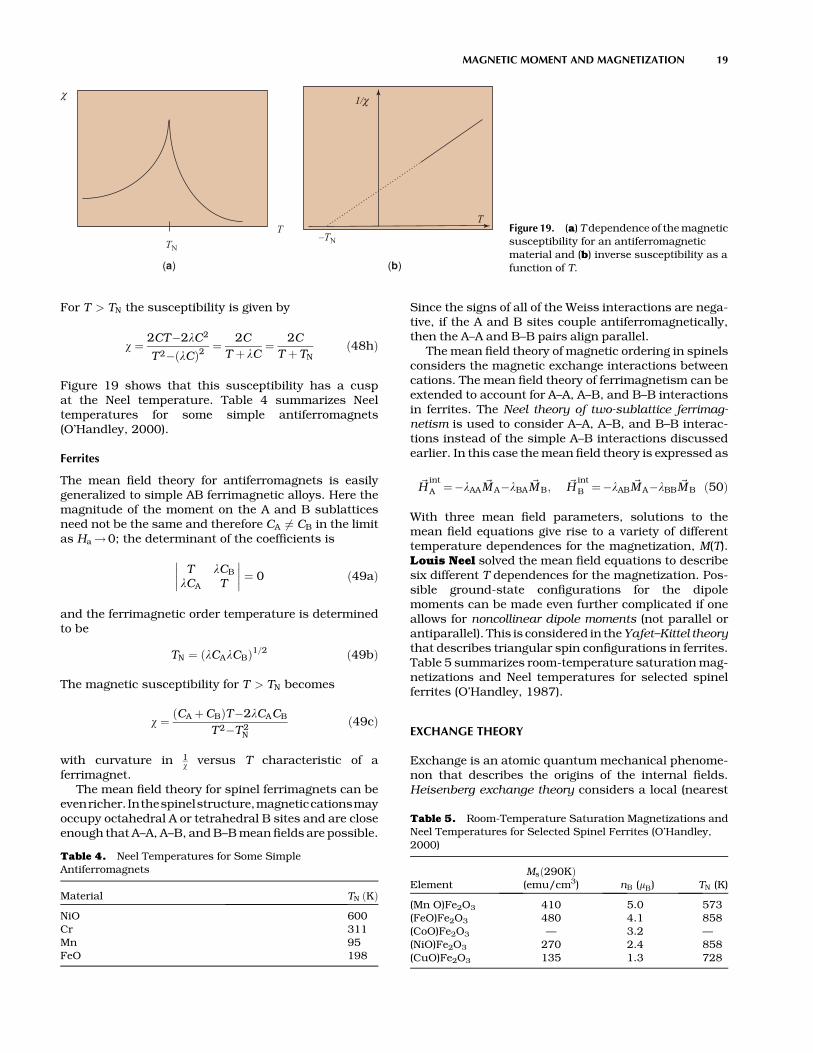
For T > TN the susceptibility is given by

w ¼ 2CT�2lC2

T2�ðlCÞ2 ¼ 2C

T þ lC¼ 2C

T þTNð48hÞ

Figure 19 shows that this susceptibility has a cuspat the Neel temperature. Table 4 summarizes Neeltemperatures for some simple antiferromagnets(O’Handley, 2000).

Ferrites

The mean field theory for antiferromagnets is easilygeneralized to simple AB ferrimagnetic alloys. Here themagnitude of the moment on the A and B sublatticesneed not be the same and therefore CA 6¼ CB in the limitas Ha !0; the determinant of the coefficients is

T lCB

lCA T

�� ¼ 0 ð49aÞ

and the ferrimagnetic order temperature is determinedto be

TN ¼ ðlCAlCBÞ1=2 ð49bÞ

The magnetic susceptibility for T > TN becomes

w ¼ ðCA þCBÞT�2lCACB

T2�T2N

ð49cÞ

with curvature in 1w versus T characteristic of a

ferrimagnet.The mean field theory for spinel ferrimagnets can be

evenricher. Inthespinelstructure,magneticcationsmayoccupy octahedral A or tetrahedral B sites and are closeenough that A–A, A–B, andB–Bmeanfields are possible.

Since the signs of all of the Weiss interactions are nega-tive, if the A and B sites couple antiferromagnetically,then the A–A and B–B pairs align parallel.

The mean field theory of magnetic ordering in spinelsconsiders the magnetic exchange interactions betweencations. The mean field theory of ferrimagnetism can beextended to account for A–A, A–B, and B–B interactionsin ferrites. The Neel theory of two-sublattice ferrimag-netism is used to consider A–A, A–B, and B–B interac-tions instead of the simple A–B interactions discussedearlier. In this case themean field theory is expressed as

~Hint

A ¼�lAA ~M A�lBA ~MB; ~Hint

B ¼�lAB ~M A�lBB ~MB ð50Þ

With three mean field parameters, solutions to themean field equations give rise to a variety of differenttemperature dependences for the magnetization, M(T).Louis Neel solved the mean field equations to describesix different T dependences for the magnetization. Pos-sible ground-state configurations for the dipolemoments can be made even further complicated if oneallows for noncollinear dipole moments (not parallel orantiparallel). This is considered in theYafet–Kittel theorythat describes triangular spin configurations in ferrites.Table 5 summarizes room-temperature saturationmag-netizations and Neel temperatures for selected spinelferrites (O’Handley, 1987).

EXCHANGE THEORY

Exchange is an atomic quantum mechanical phenome-non that describes the origins of the internal fields.Heisenberg exchange theory considers a local (nearest

TTN

–TN

T

χ 1/χ

(a) (b)

Figure 19. (a) Tdependence of themagneticsusceptibility for an antiferromagneticmaterial and (b) inverse susceptibility as afunction of T.

Table 4. Neel Temperatures for Some SimpleAntiferromagnets

Material TN ðKÞNiO 600Cr 311Mn 95FeO 198

Table 5. Room-Temperature Saturation Magnetizations andNeel Temperatures for Selected Spinel Ferrites (O’Handley,2000)

ElementMsð290KÞ(emu/cm3) nB (mB) TN (K)

(Mn O)Fe2O3 410 5.0 573(FeO)Fe2O3 480 4.1 858(CoO)Fe2O3 — 3.2 —(NiO)Fe2O3 270 2.4 858(CuO)Fe2O3 135 1.3 728


neighbor) interaction between atomic moments (spins)that acts to align adjacentmoments in the absence of anapplied field. Various types of exchange interactionsexist in materials. These can be divided into directexchange and mediated (indirect) exchange. Directexchange results from the direct overlap of the orbitalsresponsible for atomic dipole moments. Indirectexchange mechanisms include those mediated by over-lap between the magnetic orbitals and nonmagneticorbitals on the same or other species. The superex-change mechanism involves overlap between magneticorbitals and theporbitals on intervening oxygen or otheranions. RKKY interactions are those mediated throughthe conduction electrons. Exchange determines thestrength of the coupling between dipoles and thereforethe temperature dependence of the magnetization.The term random exchange refers to the weakening ofexchange interactions by disorder and its consequenteffects on the temperature dependence of themagnetization.

Heisenberg Exchange Theory

Heisenberg exchange theory (Heisenberg, 1928) consid-ers a local (nearest neighbor) interaction between atomicmoments (spins) that acts to align adjacent momentseven in the absence of a field. The Heisenberg modelconsiders ferromagnetism and the defining spontane-ous magnetization to result from nearest neighborexchange interactions that act to align spins in a parallelconfiguration. The Heisenberg model can be furthergeneralized to account for atomic moments of differentmagnitude, that is, in alloys, and for exchange interac-tions that act to align nearest neighbor moments in anantiparallel fashion or in a noncollinear relationship.Let us consider first the Heisenberg ferromagnet. Herewe assume that the atomic moments on nearest neigh-bor sites are coupled by a nearest neighbor exchangeinteraction giving rise to a potential energy:

Up ¼ Jex~Si � ~Si þ1 ð51aÞ

between identical spins at sites iand i þ 1 in a1D lattice.For identical spins:

Up ¼ �2JexS2 cosyi;i þ1 ð51bÞ

which for Jex > 0 favors parallel spins. For a linearchain of N spins (where N is large) or exploiting periodic,Born–Von Karmon BC, the total internal energy is

Up ¼ �2JexS2XNi¼1

cosyi;i þ1 ð51cÞ

which for Jex > 0 is minimized for a configuration inwhichall the spinsarealigned inaparallel ferromagneticconfiguration.

Combining mean field theory and the Heisenbergmodel, the Curie temperature can be estimated. Astatistical mechanical description of exchange hasbeen developed within the context of the Ising model.One of the results of this model allows us to associatethe exchange interaction with the Weiss molecular fieldof mean field theory. This results in the followingrelationship:

l ¼ ZJex

4Nm0m2Bð52Þ

Thus, larger exchange interactions result inhigherCurietemperatures. This allows us to use the results of meanfield theory to express the T dependence of the magne-tization. For spin-only angular momentum this is

MðT Þ ¼ M0 tanhm0mBkBT

H þ ZJexM

4Nm0mB

� �� ð53Þ

and similar expressions for the Langevin and Brillouinfunctions for classical and total angular momentummodels.

Exchange interactions result from the spatiallydependent energy functional for electrons with parallelor antiparallel spins (or canted spins in more compli-cated models). For the hydrogen molecule, for example,as shown in Figure 20a the configuration with electronspins aligned parallel is stable at larger interatomicseparations and that aligned antiparallel at smallerinteratomic separations. The choice of spin configura-tion depends on the relationship between the crossoverradius and the equilibrium separation of the atoms.

The famous Bethe–Slater curve (Bethe and Sommer-feld, 1984;Slater,1930) (Fig. 20b)predicts thesignof the

(a) (b)

Parallel

Antiparallel

2.0

1.6

1.2

0.8

0.4

0.00 1 2 3 4 5 6

r (arbitrary)

U (a

rbitr

ary)

Interatomic distance (D/d)

Exch

ange

inte

gral

γMn

α

-Fe

-FeCo

NiGd

1.5 1.75 2.0

+

−

0

2.25

Figure 20. (a) Energies for parallel andantiparallel spins in the hydrogen moleculeas a function of interatomic separation and(b) the Bethe–Slater curve predicting thesign of the exchange interaction in 3dtransition metal solids (Bethe andSommerfeld, 1984; Slater, 1930).


exchange interaction in 3d transition metal solids. Theinterplay between electron–electron Coulomb interac-tions and the constraints of the Pauli exclusion principledetermine the sign of the exchange interaction. In tran-sition metal solids a measure of the overlap betweennearest neighbor d orbitals is given by the ratio of theatomic to the 3d ionic (or nearest neighbor) radius.The Bethe–Slater curve provides an empirical descrip-tionof the exchange integral as a functionof composition(or more accurately, with interatomic spacing to 3dorbital ratio). The ratio of the 3d ionic radius to the nearneighbor distance describes the amount of orbital over-lap (or exchange).

At this point it is useful to repeat the Heisenbergmodel predictions for other magnetic ground states. Forexample, notice that if Jex < 0, an antiparallel configu-ration for adjacent spins in a 1D chain is predicted,consistent with an antiferromagnetic ground state asshown in Figure 13b. We can deduce a ferrimagneticground state as illustrated in Figure 13c and observed,for example, for ferrites when we have Jex < 0 and twomagnetic sublattices, for example, a and b, for whichma 6¼ mb. In 3D systems it is possible to relax the restric-tions of nearest neighbor exchange and it is also possibleto have noncollinear exchange interactions as shownin Figure 13d for a helimagnet. In certain ferrite systems(e.g., Mn2O3) it has been observed that Mn atoms inthe octahedral and tetrahedral sites in fcc intersticesof the oxygen anion sublattice couple in a Yafet–Kitteltriangular spin configuration (Yafet and Kittel, 1952).

Superexchange

In the context of the ferrites and other oxides we maydistinguish between direct and indirect exchange. Wehave described ferrimagnetic and Yafet–Kittel triangularspin configurations between neighboring magnetic cat-ion sites. This is an example of an indirect exchangemechanism since it must be transmitted through inter-vening nearest neighbor oxygen sites. In fact, theexchange interaction is transmitted through overlapbetween magnetic d orbitals on the cation sites and theporbitals of oxygen (Neel, 1932). This particular porbitaltransmitted indirect exchange interaction is given thename superexchange and illustrated in Figure 21.

The size of superexchange interactions depends onthedistanceandangles of thed–p–dbonds in the crystal.These are determined by the crystallography. Figure 22

illustrates the geometry of the superexchangeinteractions in the spinel structure. The strongestsuperexchange interactions occur for bond anglesapproaching 180�.

RKKY Exchange

Another form of indirect exchange has recently beenshown to be important in, for example, rare earth metalsystems and in magnetic/nonmagnetic multilayers.This exchange is the oscillatory RKKY exchange(Fig. 23a) (Ruderman and Kittel, 1954; Kasuya, 1984;Yosida, 1957) that is mediated through the conductionelectron gas often associated with nonmagnetic atomsbut sometimes associated, for example, with sp conduc-tion electrons of the magnetic atoms in rare earths. Thisindirect exchange is transmitted by polarization of thefree electron gas. The free electron sea can be charac-terized by a wavevector called the Fermi wavevector thatis defined as

kF ¼ 3p2NV

� �1=3ð54Þ

where NV is the number of free electrons per unit volume.

Examples of magnetic systems coupling throughRKKY interactions include the rare earths. In thesethe Hund’s rule ground state is determined by 4f elec-trons that are very localized, that is, close to the nucleusandshieldedbyconductionelectrons. Therefore, there isno direct exchange since 4f states do not overlapfrom site to site. Instead coupling occurs through freeelectrons. 4f dipole moments in rare earth elementspolarize the free electrons around them; these in turncommunicate the information to 4f dipole momentson adjacent sites. Coupling through the conductionelectrons is influenced by Friedel oscillations in theconduction electron spin density.

d p d

– ––

–

–

Figure 21. Superexchange interaction of magnetic cation dorbitals mediated by an O p orbital.

A site B site

AB1 AB2

0.25

0.25

0.25

0.25

0.250.22

0.22

BB1

155º135º

125º90º

BB 2

AA

HAB Large

HBB Moderate

HAASmall80º

0.29

0.44

0.44

Figure 22. Geometry of the superexchange interactions in thespinel structure.


In describing RKKY interactions we consider a polar-ization plane wave emanating from a magnetic ion at aposition r ¼ 0. The first waves influenced by a polarizingfield are those with wavevector k ¼ kF and therefore thesign of the exchange interaction oscillates spatially likecosð~kF �~r Þaswell asdecayingexponentially asa functionof r. To determine the sign of the indirect exchangeinteraction between the magnetic ion at r ¼ 0 and atr ¼ r we calculate cosð~kF �~r Þ. The RKKY exchange isweaker inmagnitude and oscillates in sign spatially andcan be described as

JRKKY ¼ J0ðrÞcosð~kF �~r Þ ð55Þ

where the prefactor J0ðrÞ decays exponentially with r.RKKY interactions are important in a variety of thin

film magnetic multilayer devices such as spin valves.These have interactions between 2D ferromagneticlayers that are coupled through a conducting layer(Fig. 23b). By varying the thickness of the conductinglayer, the sign and magnitude of the exchange interac-tion can be varied.

Random Exchange

Because of large deviations in interatomic spacings inamorphous alloys as compared with bulk crystalline,they have distributed exchange interactions that alterthe mean field description of the temperature depen-dence of the magnetization, M(T) (Chien, 1978;Kaneyoshi, 1984). A mean field theory for the T depen-

dence of the magnetization in amorphous alloys hasbeen proposed by Kobe (1969) and Handrich (1969).In this Handrich–Kobe theory was proposed an expres-sion for the reduced magnetization mðT Þ ¼ MðT Þ

Mð0KÞ thatconsisted of amodified Brillouin function where a singleexchange parameter was replaced by an exchangeparameter reflecting thedistribution of nearest neighborpositions in the amorphous phase. This is expressedas follows:

mðT Þ ¼ 1

2ðBs ð1þ dÞx½ � þBs ð1�dÞx½ �Þ ð56aÞ

where

x ¼ 3S

Sþ1

m

T; t ¼ T

Tc; d ¼

ffiffiffiffiffiffiffiffiffiffiffiffiffiffihDJ2

exihJexi2

sð56bÞ

The first expression is the argument of a conventional(spin-only) Brillouin function. The exchange fluctuationparameter, d, is defined by the second expression. Thisparameterizes the root mean square (rms) fluctuationin the exchange interaction. The root mean squareexchange fluctuation has been suggested to have a Tdependence of the form (Bhatnagar, 1984) d ¼ d0ð1�t2Þ.Figure 24a compares mean field results for M(T) in theclassical, spin-only, and total angularmomentumrepre-sentations. Figure 24b showsmean field results forM(T)taking into account the disorder-induced fluctuationsin the exchange parameter in hypothetical amorphous

1.0 1.0

0.00.0 0.00.0

0.2 0.60.2

0.20.2

0.4

0.4

0.4

0.6

0.6

0.6

0.4

0.8

0.8

0.8

0.8

J = S = 1/2

t = T/Tc t = T/Tc

δ = 0, 0.4, 0.6, 0.8J = 1/2

1.01.0

J = 7/2 (Gd3+)

J = ∞ (classical)

m =

M(T

)/M(0

)

m =

M(T

)/M(0

)

High δ

δ = 0 (crystal)

(a) (b)

Figure 24. Comparison of magnetization as afunction of reduced temperature t (a) in a spin-onlyferromagnet (using a J ¼ 1

2 Brillouin function), forJ ¼ 1

2 and for the classical limit J ¼ ‘, and (b) inan amorphous magnet with J ¼ 1

2 and differentvalues of the exchange fluctuation parameter d(figure courtesy of Hiro Iwanabe).

Ferromagnetic monolayer

Ferromagnetic monolayer

Conducting layers

k Fr

Jex

(a) (b)

5 10 15 20

+

+– – Figure 23. (a) Spatial dependence of

the RKKY exchange interaction and(b) magnetic bilayer system withintervening conducting layer thatexhibits anRKKYexchange interaction.


alloys. This construction then predicts a quite remark-able change in the mean field theory thermomagneticresponse for amorphous magnets.

The T dependence of the magnetization forFe88Zr7B4Cu amorphous alloy has been measured byGallagher et al. (1999). A two-parameter exchangefluctuation mean field theory is shown to give signifi-cantly better fits than the single-parameterHandrich–Kobe model to m(T) for these amorphousalloys. The deviation in atomic nearest neighbor (NN)distances in this amorphous alloy was estimated fromX-ray scattering data. The Bethe–Slater curve wasused to estimate fluctuations in the exchange interac-tion. An explanation for the relative invariance ofM(T) indisordered Co-based alloys as compared with Fe-basedalloys was proposed and good qualitative agreement ofthe model and experimental data has been demon-strated. The modification made to the Handrich–Kobe(Kobe, 1969; Handrich, 1969) equation allowed for two dparameters, dþ and d� (Fig. 25). The new equation is asfollows:

mðT Þ ¼ 1

2ðBs ð1þ dþ Þx½ � þBs ð1�d�Þx½ �Þ ð57Þ

where dþ and d� are not necessarily the same andtherefore can act as a first-order fit to an asymmetricdistribution function. The Gallagher (Gallagheret al.,1999) model gives a better quantitative fit to thetemperature dependence of the magnetization.

MICROSCOPIC MAGNETIZATION AND DOMAINS

A magnetic domain is macroscopic volumes over whichatomic magnetic moments are aligned. For a ferromag-net, when Ha ¼ 0, the existence of a spontaneous mag-netization requires the existence of domains. It is per-haps surprising that ferromagnetic materials can existin a “virgin state” for which the magnetization is zero inthe absence of an applied field. This is understood byferromagnetic domain theory. In a typical magnetic

material amacroscopic volume containsmanydomains.Each domain has a spontaneous magnetization of mag-nitude, Ms. In the absence of an applied field the mag-netization vectors are randomly aligned from domain todomain (just like in a paramagnet atomic dipoles wererandom). Taking a vector sum of the magnetization overmany domains yields zero sample magnetizationbecause of vector cancellation.

We can qualitatively understand this by recognizingthat magnetic flux line leaves the north pole of a magnetand enters the south pole. This gives rise to a fieldoutside themagnet, thedemagnetizationfield,Hd,whichwould like to misalign the dipole moments in the fer-romagnet. It requires internal energy to maintain thealignment of the dipoles.

A configuration for which the demagnetization field isreducedwill lower the total energy of the system. For twodomains (Fig. 26)we significantly reduce the returnpaththat is necessary to be taken by fringing fields. By apply-ing successively more domains we can further reducethe magnetostatic self-energy to nearly zero. In the casewhere we have two long domains and two closuredomains the magnetization makes a nearly circuitouspath reducing the demagnetization field to nearly zero.There is no free lunch, though. Each boundary betweendomains requires that we pay an energy associated witha domain wall. The configuration of domains and wallsultimately depends on the balancing of these twoenergies.

CONCLUSIONS

The basic notions of magnetic dipole moments andmagnetization in solids have been summarized. In par-ticular, the origin of magnetic dipoles from an atomic, aband structure, and a shielding current (superconduc-tors) picture has been described. The coupling ofmagnetic dipoles, the field and temperature dependenceof themagnetization, and simplemagnetic phase transi-tions have been illustrated. This serves to definecertain basic magnetic phenomena that will be elabo-rated on, illustrated, and extended in subsequentunits. Magnetic phenomena are rich and varied; thefundamental principles of the origin, coupling, andvector summation of magnetic dipole moments are atthe heart of a comprehensive understanding ofmagneticphenomena.

m =

m(T

)/M(0

)

1.0

t = T/Tc

0.8

1.0

0.6

0.8

0.4

0.6

0.2

0.40.20.00.0

Figure 25. Reducedmagnetization,m, as a function of reducedtemperature, t, in an amorphous Fe88Zr7B4 alloy fit withtwo asymmetric exchange fluctuation parameters, dþ and d�(Gallagher et al., 1999).

+ + + + +

- - - - -

N

S

Figure 26. Reduction in the demagnetization field as a result ofthe introduction of magnetic domains into a ferromagneticsample.


BIBLIOGRAPHY

LITERATURE CITED

Abrikosov, A. A. 1957. On the magnetic properties of super-conductors of the second group. Sov. Phys. JETP-USSR

5 (6):1174–1183.

Bhatnagar, K., Prasad, B. B. and Jagannathan, R. 1984. Phys.Rev. B, 29. 4896.

Bethe, H. A. and Sommerfeld, A. 1933. Handbuch der Physik,Vol. 24. Springer, Berlin.

Chien, C. L, 1978. Mossbauer study of a binary amorphousferromagnet: Fe80 B20, Phys. Rev. B. 18:1003–15.

Cullity, B. D. and Graham, C. D. 2009. Introduction toMagnetic Materials, 2nd ed. IEEE Press/John Wiley andSons, Hoboken, NJ.

de Gennes, P. G. 1966. Superconductivity of Metals and Alloys.Benjamin, New York.

Diaz-Michelena, M. 2009. Small magnetic sensors for spaceapplications. Sensors 9:2271–2288.

Diggs, B., Zhou, A., Silva, C., Kirkpattrick, S., McHenry, M. E.,Petasis, D., Majetich, S. A., Brunett, B., Artmen, J. O., andStaley, S. W. 1994. Magnetic properties of carbon-coatedrare earth carbide nanocrystals produced by a carbon arcmethod. J. Appl. Phys. 75:5879.

Fisher,M.P.A.1989.Vortex-glass superconductivity: Apossiblenew phase in bulk high-Tc oxides. Phys. Rev. Lett. 62:1415.

Friedel, J. 1958. Theory of magnetism in transition metals.Nuevo Cim. Suppl. 7:287.

Gallagher, K. A., Willard, M. A., Laughlin, D. E., andMcHenry, M. E. 1999. Distributed magnetic exchange inter-actions and mean field theory description of temperaturedependent magnetization in amorphous Fe88Zr7B4Cu1

alloys. J. Appl. Phys. 85:5130–5132.

Ginzburg, V. L. and Landau, L. D. 1950. Zh. Eksp. Teor. Fiz.20:1044.

Handrich, K. 1969. A Simple Model for Amorphous and LiquidFerromagnets. Phys. Status Solidi. 32:K55.

Harrison, W. A. 1989. Electronic Structure and the Propertiesof Solids: The Physics of the Chemical Bond. DoverPublications, New York.

Heisenberg,W. 1928.On the theory of ferromagnetism. Z. Phys.49:619.

Hund, F. 1927. Linienspektren und periodische system derelemente. Springer, Berlin.

Kammerlingh-Onnes,H.andTuyn,W.1929.LeidenComm.198.

Kaneyoshi, T. 1984. Amorphous Magnetism Chemical RubberCorp., Boca Raton, FL.

Kasuya, T. 1956. Electrical resistance of ferromagnetic metals.Prog. Theor. Phys. 16:45.

Kobe, S. 1969. Phys. Status Solidi. 32:K55.

Kobe, S. 1970. ibid. 41:K13.

Kobe, S., Handrich, K., Tverd, Fiz. and Leningrad, Tela. 1971.13, 887 and Sov. Phys. Solid State. 13:734.

Langevin, P. 1907. Magnetisme et Theorie des Electrons. Ann.Chem. Phys. 5:70.

London, F. 1950. Superfluids, Vol. 1. John Wiley and Sons,New York.

MacLaren, J. M., McHenry, M. E., Eberhart, M. E., andCrampin, S. 1990. Magnetic and electronic properties ofFe/Au multilayers and interfaces. J. Appl. Phys. 61:5406.

MacLaren, J. M., Schulthess, T. C., Butler, W. H., Sutton, R. A.,andMcHenry,M.E.1999.CalculatedExchange Interactionsand Curie Temperature of Equiatomic B2 FeCo. J. Appl.

Phys. 85:4833–35.

Maley, M. P., Willis, J. O., Lessure, H., and McHenry, M. E.1990. Dependence of flux creep activation energy uponcurrent density in grain-aligned YBa2Cu3O7-x. Phys. Rev.B 42:2369.

McHenry, M. E. andMacLaren, J. M. 1991. Iron and chromiummonolayer magnetism in noble-metal hosts: Systematicsof local moment variation with structure. Phys. Rev. B

43:10611.

McHenry,M.E.,MacLaren, J.M.,Eberhart,M.E., andCrampin,S. 1990. Electronic and magnetic properties of Fe/Au multi-layers and interfaces. J. Magn. Magn. Met. 88:134.

McHenry, M. E. and Sutton, R. A. 1994. Flux pinning anddissipation in high temperature oxide superconductors.Prog. Met. Sci. 38:159.

Meissner, W. and Ochsenfeld, R. 1933. Ein neuer Effekt beiEintritt der Supraleitfahigkeit. Naturwissenschaften

21:787–788.

Neel, L. 1932. Influences des Fluctuations du Champ Molecu-laire sur les Proprietes Magnetiques des Corps. Ann. Phys.18:5–105.

Nelson, D. R. 1988. Phys. Rev. Lett. 60:1973.

Onnes,H.K.1911.Thesuperconductivityofmercury.Commun.

Phys. Lab. Univ. Leiden 122, 124.

Onnes, H. K. andClay, J. 1908. On the change of the resistanceof themetals at very low temperatures and the influence on itby small amounts of admixtures. Commun. Phys. Lab. Univ.

Leiden 99c:17–26.

O’Handley, R. C. 1987. Physics of ferromagnetic amorphousalloys. J. Appl. Phys. 62 (10):R15–R49.

O’Handley, R. C. 2000. Modern Magnetic Materials, Principlesand Applications. John-Wiley and Sons, New York.

Pauling, L. 1938. The nature of the interatomic forces inmetals.Phys. Rev. 54:899.

Ruderman, M. A. and Kittel, C. 1954. Indirect exchangecoupling of nuclear magnetic moments by conductionelectrons. Phys. Rev. 96:99.

Russell, H. N. and Saunders, F. A. 1925. New regularities in thespectra of the alkaline earths. Astrophys. J. 61:38.

Slater, J. C. 1930. Atomic shielding constants. Phys. Rev.

36:57–64.

Slater, J. C. 1937. Electronic structure of alloys. J. Appl. Phys.8:385.

Van Vleck, J. H. 1932. The Theory of Electric and MagneticSusceptibilities. Oxford University Press, New York.

Weiss, P. 1907. L’hypothese du Champ Moleculaire et laPropriete Ferromagnetique. J. Phys. 6:661.

Yafet, Y. and Kittel, C. 1952. Antiferromagnetic arrangementsin ferrites. Phys. Rev. 87 (2):290–294.

Yosida, K. 1957. Magnetic properties of Cu–Mn alloys. Phys.Rev. 106:893.

KEY REFERENCES

Solid State Physics Texts—Introductory (Undergraduate)Level

Eisberg, R. and Resnick, R. 1974. Quantum Physics of Atoms,

Molecules, Solids, Nuclei and Particles. JohnWiley and Sons,

New York.


Rosenberg, H. M. 1990. The Solid State. Oxford Science Publica-

tions, Oxford.

Solymar, L. and Walsh, D. 1998. Lectures on the Electrical

Properties of Materials. Oxford University Press, New York.

Solid State Physics Texts—Intermediate to Graduate LevelAshcroft,N.W.andMermin,N.D. 1976.SolidStatePhysics.Holt,

Rinehart and Winston, New York.

Blakemore, J. S. 1981. Solid State Physics. Cambridge Univer-

sity Press, Cambridge, UK.

Burns, G. 1985. Solid State Physics. Academic Press, SanDiego,

CA.

Kittel, C. 1976. Introduction to Solid State Physics. John Wiley

and Sons, New York.

Physics of MagnetismChikazumi, S. 1978. Physics of Magnetism.Kreiger,Malabar, FL.

Keefer, F. 1982. Helimagnetism. In McGraw-Hill Encyclopedia

of Physics (S. P. Parker, ed.). McGraw-Hill, New York.

Morrish,A.H.1965.ThePhysicalPrinciplesofMagnetism.Wiley,

New York.

Mydosh, J.A. 1993.SpinGlasses,AnExperimental Introduction.

Taylor and Francis, London, Washington, DC.

White, R. M. 1983. Quantum Theory of Magnetism, Springer

Series in Solid State Physics 32. Springer-Verlag, Berlin.

Magnetic Materials

Berkowitz, A. E. and Kneller, E. 1969. Magnetism and

Metallurgy, Vol. 1. Academic Press, San Diego, CA.

Bozorth, R. M. 1951. Ferromagnetism. Van Nostrand,

New York.

Chen, C.-W. 1986. Metallurgy of Soft Magnetic Materials. Dover,

New York.

Coey, J. M. D. 2010. Magnetism and Magnetic Materials,

Cambridge University Press, Cambridge.

Cullity, B. D. 2009. Introduction to Magnetic Materials, 2nd ed.

IEEE Press, Hoboken, NJ.

Kouvel, J. S. 1969.MagnetismandMetallurgy 2 (A. E. Berkowitz

and E. Kneller, eds.), p. 523. Academic Press, New York.

McCurrie, R. A. 1994. Ferromagnetic Materials: Structure and

Properties. Academic Press, London.

Morrish, A. H. 2001. The Physical Principles of Magnetism. IEEE

Press, New York.

O’Handley, 2000. See above.

Fine Particle and NanomagnetismBean, C. P. and Livingston, J. D. 1959. J. Appl. Phys.

30:120S–129S.

Bitter, F. 1932. Phys. Rev. 38:1903; ibid. 41:507 (1932).

Jacobs, I. S. and Bean, C. P. 1963. Magnetism, Vol. 3 (G. T. Rado

and H. Suhl, eds.). Academic Press, New York.

Luborsky, F. E. 1962. J. Appl. Phys. 32:171S–183S.
