magneto-hydro-dynamic waves in the collisionless space plasma

Sun and Geosphere, 2007; 2(2): 65 - 77 ISSN 1819-0839

65

Magneto-Hydro-Dynamic Waves in the Collisionless Space Plasma

N.S. Dzhalilov 1, V.D. Kuznetsov 2, J. Staude 3

1 Shamakhy Astrophysical Observatory (ShAO) named after N.Tusi,

Azerbaijan National Academy of Sciences, Baku, Azerbaijan

e-mail: [email protected]

2 Pushkov Institute of Terrestrial Magnetism, Ionosphere and Radio Wave Propagation (IZMIRAN),

Russian Academy of Sciences, Troitsk, Moscow Region, Russia 3 Astrophysicalisches Institut Potsdam (AIP), Potsdam, Germany

Received: 15 October 2007; Accepted: 10 December 2007

Abstract. The instability of magneto-hydro-dynamic (MHD) waves in an anisotropic, collisionless, rarefied hot plasma is studied. Anisotropy properties of such a plasma are caused by a strong magnetic field, when the thermal gas pressures across and along the field become unequal. Moreover, there appears an anisotropy of the thermal fluxes. The study of the anisotropy features of the plasma are motivated by observed solar coronal data. The 16–moments equations derived from the Boltzmann-Vlasov kinetic equation are used. These equations strongly differ from the usual isotropic MHD case. For linear disturbances the wave equations in homogenous anisotropic plasma are deduced. The general dispersion relation for the incompressible wave modes is derived, solved and analyzed. It is shown that a wide wave spectrum with stable and unstable behavior is possible, in contrast to the usual isotropic MHD case. The dependence of the instability on magnetic field, pressure anisotropy, and heat fluxes is investigated. The general instability condition is obtained. The results can be appliedto the theory of solar and stellar coronal heating, to wind models and in other modeling, where the collisionless approximation is valid.

2007 BBSCS RN SWS. All rights reserved.

Keywords: MHD waves, collisionless space plasma, anisotropy, instability, coronal heating

1. Introduction Since the first identification of the coronal emission

lines as forbidden lines of multiply ionized atoms (Fe, Ni)by Grotrian [1] and Edlén [2] it has been recognized that the corona has a high temperature of T > 106 K and requires permanent heating. Heating by acoustic waves was first proposed by Biermann [3]. Later the idea has been extended to magneto-hydro-dynamic (MHD) waves because heating seems to be focused to regions with magnetic field concentrations, to closed fields in particular. Parker [4, 5] suggested heating by currents due to topological dissipation of magnetic fields braided by photospheric footpoint motions. So far a huge number of interesting heating mechanisms have been suggested, but it turned out to be difficult to select and prove the most probable mechanisms by existing observations. Recently, new excellent space-borne data became available; simultaneously the plasma physics simulations and MHD modeling in particular have reached a degree of realism which suggests to look again for a solution of the problem. For example, Aschwanden et al [6] gave 10 arguments against local heating in the corona, but in favor of primary heating in

the upper chromosphere and transition region, in the footpoint regions of closed magnetic loops.

Our knowledge of coronal loop oscillations has greatly improved by imaging observations, mainly onboard the SOHO and TRACE satellites [7]. Different kinds of strongly damped oscillation modes are observed as transverse amplitude oscillations with periods of 2 – 30 min. By imaging radio measurements modes with much shorter periods are detected. The great variety of waves and oscillations observed in detail in the corona [7, 8] suggests to consider wave heating again. Acoustic waves are damped in the lower chromosphere. MHD waves, transverse incompressible Alfvén waves in particular, can travel along the magnetic field, reach coronal heights and bring enough energy to these heights. However, it is difficult to convert globally this energy into heat. In order to increase the dissipation various mechanisms of damping of such waves have been suggested (see [9]), such as phase mixing, resonant damping, coupling to compressible (slow and fast) MHD modes, and kinetic effects (ion-cyclotron resonance). The coronal emission lines arising practically at all altitudes with different magnetic configurations demonstrate a non-thermal broadening of the profiles. From Doppler shift estimates the amplitudes of such

N.S. Dzhalilov, et al. MHD Waves in the Collisionless Space Plasma

66

motions are in the range of 25 – 50 km s 1. The origin of such turbulent motions is unclear.

The coronal plasma is very anisotropic and inhomogeneous, in cross-field direction in particular [7]. Various topologies of a strong magnetic field with open and closed configurations in an almost collisionless, rarefied, hot space plasma lead to its strong anisotropy, and the transport coefficients become tensor quantities. Under such circumstances a traditional hydro-dynamical description of the plasma is impossible. That is why we try to extend the MHD equations by considering the anisotropy of the magnetized collisionless plasma.

Let us consider, for instance, the characteristic parameters of the solar corona: a temperature of Te Ti = 106 K, a density of ne np = 109 cm 3 (subscripts e, i, and p mark values for electrons, ions, and protons, respectively), and a range of magnetic field strengths of B = 0.1 100 G. Using these parameters we get the following estimates: electron and ion thermal velocities of Tev 4 × 103 km s 1 and Tiv 100 km s 1, electron and

ion collision times of e 10 2 s and i 0.8 s, electron

and ion mean free paths of e 40 km and i 80 km,

electron and ion gyroradii of Ber 200 0.2 cm and Bir9000 9 cm, electron and ion gyrotimes of Be

10 6 10 9 s and Bi 10 2 10 5 s, Alfvén and sound

speeds of Av 10 104 km s 1 and Sc 100 km s 1,respectively. Hence the conditions of a strong magnetic field — e » Ber , i » Bir , e » Be , and i » Bi — are well satisfied. That means, particles gyrating around the magnetic field lines are localized across the field at a distance of the Larmor radius which for motions across the magnetic field plays the role of a free path length of particles. Thus the dynamical motion of a collisionless plasma with characteristic scales of L » Br and » Bbehaves across the magnetic field as a fluid.

Frequent collisions turn the plasma distribution function to an isotropic one, and thus the thermal pressure is isotropic as well. If collisions rarely occur, the energies of chaotic motions are no longer “mixed”, and pressure becomes anisotropic. The presence of a magnetic field will maintain a “non-mixed” state of the energies of longitudinal and transverse motions of particles. So, the transverse and longitudinal pressures will differ from each other, 1|||| TTpp (here

p and T are the mean thermal pressure and

temperature). For a very short time Be across the magnetic field mean values of thermal pressure and temperature are established, but this does not occur so fast along the field. As a result the plasma becomes colder along the magnetic field, TT|| . A distinct

thermal anisotropy of 32~||TT has been observed in

the solar wind, see for example, Feldman et al [10], Marsch et al [11], and Casper et al [12]. A strong anisotropy of temperature of the ionospheric plasma

reaching 50-60 percent is really found in experiments, see Clark et al [13] and Likhter et al [14]. Large heavy-ion thermal anisotropies ( 100||TT ) were also detected in

the solar corona by UVCS/SoHO by Kohl et al [15] and Cranmer et al [16]. A similar but smaller anisotropy exists for protons, see Cranmer et al [16], and for the coronal hole temperature anisotropy, see Dodero et al [17] and Antonucci et al [18]. It is now generally accepted that the observed large ion temperature anisotropies are related to the physical mechanism by which the solar corona and solar wind are heated, see Hollweg and Isenberg [19], and Marsch [20].

Along the magnetic field the plasma is collisionless, if the particle parallel mean free path is not small in comparison with the considered characteristic scales:

ie, 50 km, so that the wavelength along the

magnetic field is || < 50 km. The hydro-dynamical

description can also be applied to the motions of such a plasma. The criterion of applicability of the hydro-dynamical description in this case is obtained by comparing self-consistently the electric force with the pressure gradient; it is connected with the smaller thermal velocity of particles in comparison with the speeds of the directed stream: AT vvv ~0

21 , see Oraevskii et al [21].

Due to the anisotropy of the kinematic temperatures of protons and heavy ions the corresponding partial pressures become anisotropic in this way. This makes the total thermal pressure anisotropic too,

||pp . Physically

such a situation can be realized only if the particle collisions in the plasma are rare. In the present paper we consider the wave peculiarities which can appear in a collisionless plasma. With this objective we formulate in Section 2 the basic equations, which are the integrated moments’ equations of the kinetic Boltzmann-Vlasov equation. In Section 3 the linear wave equation and the general dispersion relation for the incompressible case are derived. The solutions and analyzes of the dispersion equation are the topic of Section 4. In Section 5 we investigate the instability domains in dependence on the magnetic field, on the pressure anisotropy parameter, and on thermal fluxes. The discussion and conclusions are presented in Section 6. In the Appendix the common expression describing the boundaries of the instability domains is derived.

2. Basic Equations A successful way to describe a plasma is the use of

the system of the equations consisting of the kinetic equations for the distribution functions of the particles and the Maxwell equations for the electromagnetic field. The hydro-dynamical approach is based on the isotropic character of the distribution of the degrees of freedom of thermal energy for the plasma components in the form of (or very close to) the Maxwell function. However, in real situations the distribution functions of the space plasma components, ions in particular, differ strongly from the Maxwell function.

Despite the relative smallness of Tie,

« 1 ( T is the

thermal scale height), the coronal plasma, for example,


67

cannot be described satisfactory by theories supposing that local velocity distribution functions are close to Maxwellians, see Marsch [20].

The distribution function trufa ,, describes the density of particles of a kind a in the six-dimensional phase space ru, ; it is the solution of the kinetic Boltzmann-Vlasov equation:

aauaaaa

aaa QfBu

cEeF

mfu

tf 11 (1).

Here E and B are the total electric and magnetic fields, ae and am are the charge and mass of particles

of a sort a , aF are the non-electromagnetic forces; c is

the speed of light, u is the gradient in the velocity

space, and aa fQ are the integrals of collisions. This statistical equation for the plasma is deduced assuming that the ratio of the average energy of the interaction of two particles to their average kinetic energy is small enough. That means the number of particles in a plasma sphere with a Debye radius Dr should be 31 Dnrg « 1.

In a collisionless approach 0aQ . The left-hand part of Eq. (1) gives an effect of the order of unity, while the right-hand part for pair collisions (Landau integrals of collisions), for example, gives an effect of order g [22]. For coronal conditions g 10 6, hence the collisionless approach can be applied. All the macroscopic parameters (density, plasma flow speed, pressure, thermal flux, tensor of viscosity, etc.) are defined as the corresponding speed moments of the distribution function:

k

j jak

kk vfdutrMM

1 ,)(...1 ),( , 3,2,1i .

For example, the density of particles is udftrnn ),( , the hydro-dynamical speed of the

plasma is udfutrvn ),( , where zyx dududuud .

Due to the complexity of Eq. (1), usually the equations for the moments of the distribution function are deduced, and these equations refer to the hydro-dynamical or the transport equations. The main difficulty in deducing these transport equations consists in the problem that in the infinite chain the momentum equations become coupled among each other, therefore some additional physically proved assumptions for truncating this chain are required.

In a collision dominated plasma one can decompose the distribution functions around the basic state of an isotropic equilibrium which is described by the Maxwell function, and if hydrodynamics can be applied a truncation of the chain of moment equations leads to rather simple MHD equations. If collisions among particles are rare and a strong magnetic field is present, the conditions become more complicated, however, for a collisionless plasma mainly across a magnetic field the hydro-dynamical approach can be used, see, e.g., Chew et al [23], and Rudakov and Sagdeev [24]. In this approximation the distribution function in a strong

external magnetic field will depend on both speeds, those along and across the field:

),,,(),,( || tuurfturf .

The solution of the kinetic equations is searched for in the form of the expansion

vk

kvv truPtratruftruf

,

)(0 ),,,(),(),,(),,( (2)

where 0f is the weighting function of the expansion (the

zero-approach distribution function), va are the

expansion coefficients, v are the coordinates, )(kP is an orthogonal polynomial of order k (for example, a Hermitian polynomial). If a Maxwellian distribution is chosen for the weight function 0f , Eq. (2) describes a state close to the thermodynamic equilibrium. Such an approach refers to the method of Grad [25]. However, the method of Grad cannot be applied to describe a plasma with arbitrary anisotropic pressure. For this purpose Oraevskii et al [26, 21] have used a bi-Maxwellian quasi-equilibrium distribution,

.22

exp22 ||

2||

221

||0 kT

mukT

mukTm

kTmnf (3)

For a small parameter 0g the plasma is closer to a thermo-dynamical equilibrium state. In that case the multi-partial distribution function is close to a product of single partial distribution functions [22]. Therefore it is justified to use a bi-Maxwellian distribution calculated by multiplying the two functions along the magnetic field and across the field. This method introduces two vectors of thermal fluxes, and the total distribution function is expressed through 16-moments. The method of Grad results in 13–moments equations. The conditions for truncating the chain of the equations to the 16–moments equations are reduced to the following two statements:

a) the components of the viscosity tensor should be much smaller than the pressures across and along the field, ||, pp ;

b) thermal fluxes ||, SS « 3Tv , where mkTvT is

the thermal speed. These requirements are satisfied in the transverse

direction, if LrB « 1, B « 1. In the longitudinal

direction we should have |||| Lva TII «1. 0||ameans small pressure forces (thermal motion of particles) in comparison with the electromagnetic forces, i.e. the plasma is “cold”. In this case the equation of motion is transformed into the equations of motion for the separate components of the plasma.

The 16–moments set of equations was used by many authors in different theoretical approaches, especially for modeling the solar wind, see Demars and Schunk [27], Olsen and Leer [28], Li [29], and Lie-Svendsen et al [30]. Thus, the 16–moments set of transport or MHD (not in the sense of the usual isotropic case) equations for the collisionless plasma in the presence of gravity g but


68

without magnetic diffusivity under the conditions of B «

V , B « Tv is given as follows, see Oraevskii et al [21]:

,0divvdtd (4)

,][

41

8

||||

2

pphhhhhdivhpp

gBBBpdtvd

(5)

,2||3

2

3

2|| Bh

BS

BS

hBBBpdtd (6)

,2BShB

Bp

dtd (7)

,3 ||

4

3||

4

3|| p

hBpBS

dtd (8)

,||

||2||

2 BhBppppph

pSdtd (9)

,0vBvdivBdtBd ,0Bdiv (10)

where ,|| ,|| hh and

,vtdt

d ,|| vvvBBh (11)

Here ||S and S are the heat fluxes along the

magnetic field by parallel and perpendicular thermal motions. If the thermal fluxes are neglected, S = 0 and

||S = 0, we receive the equations describing the laws of

the change of longitudinal and transverse thermal energy along the trajectories of the plasma (the left-hand parts of Eqs. (6) and (7). These so-called “double-adiabatic” parities and Eqs. (4), (5), and (10) form as though a closed system of equations, the CGL (Chew-Goldberger-Low) equations, see Chew et al [23]. However, using the CGL-equations can result in unsatisfactory Eqs. (8, 9). This is because deducing the CGL equations the third moments of the distribution function, hence the thermal fluxes, have been lost without any proof, see Chew et al [23], and Baranov and Krasnobayev [31]. The equations following from the 16–moments set in our case, Eqs. (4 - 10), consider the thermal fluxes, they are more complete, and the CGL equations do not follow from these equations as a special case. One should compare the final results in the limits S 0 and ||S 0 with the results based on the

CGL equations, deduced by many authors, see, e.g., Kato et al [32], Baranov and Krasnobayev [31], and Kuznetsov and Oraevskii [33].

3. Wave equations For simplicity we will now assume, that the basic initial

equilibrium state of the plasma is homogeneous, g = 0, and the following quantities are constant:

,,,,,, 000||00 SBppv o and 0||S . Eqs. (4–10) will

automatically satisfy such an equilibrium state with non-

zero thermal fluxes. We will consider small linear perturbations of all physical variables, e.g. for pressure in the form ).,(0 trppp

Let ,exp~),( trkitrp where kv00

is the wave frequency observed in the moving frame of the fluid, and k is the wave number of the fluctuations. For the perturbations we receive the equations

00 vk (12)

,0

44

||00

000

pphkhkhkh

BBkBBpkv (13)

,000 vBkvkBB ,0Bk (14)

,0

20

10

0 aBBa

ppa (15)

.0

20

10||

||0 b

BBb

pp

b (16)

Deriving these equations we have excluded fluctuations of the thermal fluxes, using

,20

000||000

00|| SBB

pppppk

S (17)

.433

000||

00||

||

0

20||

|| BBS

ppkp

S (18)

Here ,00|| pp ,000 BBhcos0* kkhk . The indices II and correspond

to the values of the parameters along and across the magnetic field. Even if we insert in Eqs. (17–18)

,000|| SS the perturbations of these functions will

never become zero: 0,0|| SS . That means, using

the 16–moments equations we should get more reliable results on the wave properties in an anisotropic plasma than with the CGL equations based on the 13–moments equations.

Strictly speaking, the heat fluxes of particles of a kind a should be defined as ,2

21

aaaaa ccmnS where

aa vuc is the chaotic thermal speed. In the presence of an external magnetic field the components of this flux are defined by the solutions of the kinetic Eq. (1). However, we should use here some appropriate estimate as a parameter.

The initial collisionless heat flux functions 0||S and 0Sshould be estimated by taking the thermal energy density of the electrons multiplied by the non-thermal flow speed along the magnetic field

0v :

.43

23

||00||0|| pvvTknS Be

Hollweg [34, 35] has given some estimates of the correction parameter ( in his papers) assuming various realistic shapes of the electron distribution function in Eq. (1) and checking the results for


69

agreement with space observations. depends on the magnetic field. In the range of B = 0.1 100 G we have

4 0.1. In the same way pvS 00 43 . Using the

condition 3||,||, )( TvS mentioned above, we get

some restriction for 0v : 30

2Tes vvc . Even for the

maximum Alfvén velocity Avv0 this condition is

obeyed. For coronal conditions we should identify 0vwith the observed non-thermal velocities which follows from the broadening of spectral lines: ~ 30 50 km s 1.

Let us introduce dimensionless parameters (in the further text indexes “0” of physical parameters will be omitted for simplicity):

,cos,4

,,1,

||||||2||

2

||

2

||2||

||

kckccv

pB

pc

pp

A

(19)

,,||||||

|||| cp

SScp

SS

22

21|| sin,cos,2 llSSS (20)

Note that is defined here inversely proportional to the often used “plasma beta”. By means of these parameters the coefficients 2,1,0a and 2,1,0b are defined

as2

12

0 21,1 Saa , (21)

,21 22 Sa (22)

.343,2,31 2||21

20 SbSbb (23)

Having excluded and P from Eqs. (12-16) we receive

,02

41

0

2

0

2

0

1

0

1

0

2

0

1

||

vkaa

bb

BB

aa

bb

BB

BB

pBBvk

aa

BB

aa

kk

cv

(24)

.0,0 BkvkvkBB

BB (25)

The k - and B -components of these vector equations are given by

,02

411

0

1

0

2

1

2

||10

2

0

2

1

22

BB

bb

aa

ll

pBB

lvk

bb

aa

ll

(26)

,021

0

12

0

2

|| BB

bb

BBBvk

bb

BcvB (27)

.0,02||

BkB

BBvkBc

vB (28)

In analogy to usual MHD as used by Somov et al [36], there are two independent wave branches in the plasma: waves which do not compress the plasma ( 0vdiv ), and waves compressing the plasma ( 0vdiv ). In this paper we shall restrict ourselves to the wave modes uncompressing the plasma.

Having inserted in Eqs. (26–28) the condition of incompressibility 0vk , and excluded the variables

vB and BB we receive

Fig. 1. Increment/decrement of the instability normalized to as a function of the anisotropy parameter in the

domain of the instability (left picture). In the right picture the phase velocity of the unstable modes |||| ckRV eph

normalized to is shown. The numbers on the curves are values of the propagation angle . These figures are asymptotic

limit cases of unstable solution of Eq. (31).


70

.02

12

0

1

20

1

0

11

0

1

BB

bb

BB

aa

bbl

aa

(29)

As far as 0B the dispersion relation must be fulfilled:

.02120

12

0

1

0

11

0

1

bb

aa

bb

laa (30)

This is a polynomial equation of 6th order in the frequency of the fluctuations. For the parameter

||||1 kcZ this equation can be written in the

form,001

22

33

44

55

66 cZcZcZcZcZcZc (31)

where

126215

2114

21123

2112

121

120

2,2,234

,223,4234,223

,23

llcllclllc

llllclllc

llcllc

Here the dimensionless parameter ||043 cv is

introduced, by which the heat fluxes are defined: .2,|| SSS In the usual isotropic MHD

case only the Alfvén waves with 22||

2Avk can arise,

the phase velocities of which are equal to each other in both directions with respect to the magnetic field. So, instead of 2Z in the isotropic MHD we have deduced now the 6-th order Eq. (32) in the anisotropic MHD. With the non-zero heat fluxes 0 , odd non-zero

coefficients 531 ,, ccc will result in wave propagation velocities depending on the direction of the magnetic field. We can expect prograde and retrograde wave modes. Let us first consider the most important limit cases of Eq. (32) which can be solved analytically.

4. Limit cases 4.1. Strong magnetic field

Let us consider the case 2||

2 cva or the limit

. Using the usual asymptotic expansion we find the six solutions of Eq. (31):

12

211

6

5

6

21

2,1 cc

ciZ (32)

Here 1 and 06c should be obeyed. In the case

1we have 22 cos12Z .That means, 22

||2

Avk along the magnetic field,

0 , and 22||

2 2 Avk across the magnetic field,

2 . In the opposite case 1 we get an

analogy to the inclined Alfvén waves, 222Avk . So,

the solution (32) describes the prototype of the usual (isotropic) Alfvén waves. But for more realistic values of the anisotropy parameter )1(~ O these mode becomes unstable. The instability condition is

1cos1cos2

2

2 (33)

Instability does not arise for waves propagating along the magnetic field, 0 . The growing time increases with the magnetic field and does not depend on . The second term in Eq. (32) defines the phase velocity of the unstable modes, which is independent from the magnetic field, but it depends strongly on . The instability increment and the phase velocity are defined

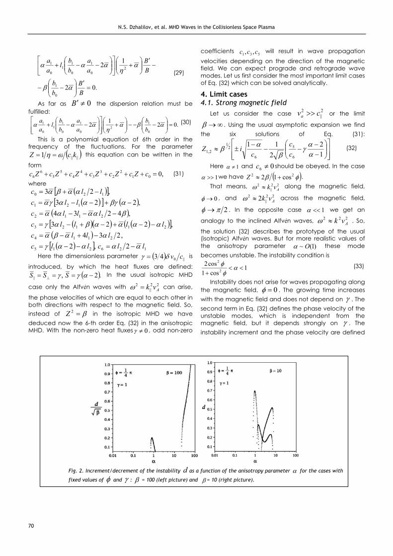
Fig. 2. Increment/decrement of the instability d as a function of the anisotropy parameter for the cases with

fixed values of and : = 100 (left picture) and = 10 (right picture).


71

as

.)1(4)34()Re(

,)34(

114)Re()Im(

6

2

||||

26

cl

ckV

lcd

ph

(34)

d has both signs and Vph > 0, the unstable modes are running along the magnetic field. In Figs. 1 these parameters are shown in the instability range of . The instability growing increment (or damping decrement) has rather high values. The maxima of d correspond to the minima of the phase velocities. For more inclined modes d becomes larger and the minima of Vph

decrease. From the figures for different values of and the increments and phase velocities can easily be

estimated. The other solutions of Eq. (31) present stable waves,

,1:0)Im( 4,3Z

1211222 222

6,5Z (35)

The first one is practically a symmetric slow wave with .|| Ahp vcV The second solutions are strongly

asymmetric stable waves, Vph > 0 means prograde waves, Vph < 0 retrograde waves. For < 1 we have Z5 > 0, that means prograde waves, and Z6 < 0 retrograde ones. In this case |Z6| > |Z5|, that means retrograde waves are faster. For > 1 we get the opposite case: Z5

< 0 and Z6 > 0. In the range 1 < < 2 prograde waves are faster, |Z6| > |Z5|, and for > 2 we have |Z5| > |Z6|. =2 is a symmetric case, |Z5| = |Z6|. Anti-symmetric features of waves are due to thermal fluxes. If the thermal fluxes are not included, = 0, both waves have the same velocities, such as in the isotropic case. We found analytically the asymptotic solutions of Eq. (31) for . In this case only one pair of solutions is complex and can become unstable.

Fig. 3. Increment/decrement of the instability d as a function of the anisotropy parameter for the cases with fixed values of

and : = 1 (left picture) and = 0.1 (right picture).

Fig. 4. Two characteristic cases of phase velocity ||||)Re( ckVhp as a function of the anisotropy parameter for the cases with

fixed values of and : = 1 (left picture) and = 100 (right picture).


72

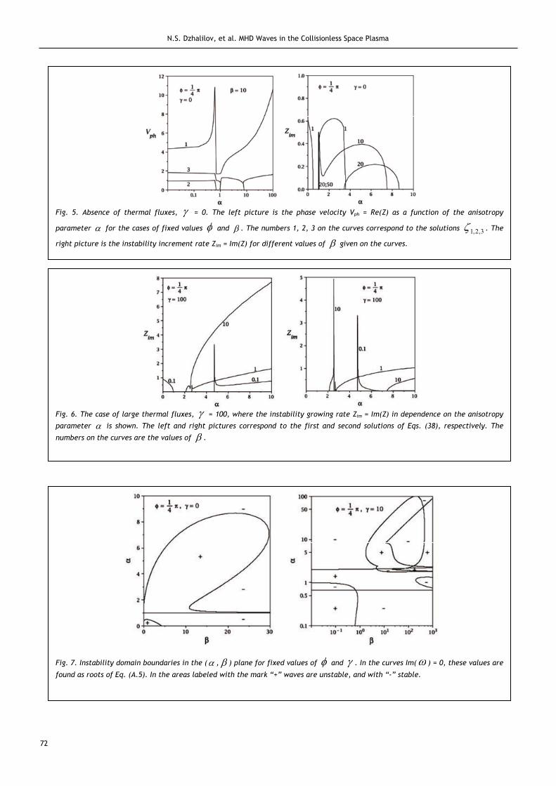
Fig. 7. Instability domain boundaries in the ( , ) plane for fixed values of and . In the curves Im( ) = 0, these values are

found as roots of Eq. (A.5). In the areas labeled with the mark “+” waves are unstable, and with “-” stable.

Fig. 6. The case of large thermal fluxes, = 100, where the instability growing rate Zim = Im(Z) in dependence on the anisotropy

parameter is shown. The left and right pictures correspond to the first and second solutions of Eqs. (38), respectively. The

numbers on the curves are the values of .

Fig. 5. Absence of thermal fluxes, = 0. The left picture is the phase velocity Vph = Re(Z) as a function of the anisotropy

parameter for the cases of fixed values and . The numbers 1, 2, 3 on the curves correspond to the solutions 3,2,1 . The

right picture is the instability increment rate Zim = Im(Z) for different values of given on the curves.


73

Let us take from Figs. 1 one characteristic case, say = 0.25 and =1. For this case the exact numerical solutions of Eq. (31) can be found. The cases = 100, 10, 1, and 0.1 are demonstrated in Figs. 2 and 3, where the increments of the unstable waves are shown.

For moderate values of all the solutions become complex. For > 300 the picture of instability tends to the asymptotic case as shown in Fig. 1. In these figures we see only three roots of the polynomial equation. The other three roots are symmetric with negative sign. Two characteristic cases of phase velocities are shown in Figs. 4. For small and large values of the solutions are more symmetric, prograde and retrograde modes have more or less the same velocities. Waves with |Vph| 1 practically exist in all cases. A more complicated case is the range 1 < < 2, where the anisotropy of the modes is strong. An anisotropic propagation of waves is a consequence of the thermal fluxes. Let us consider the two limit cases, 0 and , analytically.

4.2. Special case 0 Although the absence of fluxes, 0S and 0||S ,

is far from reality, this simplified case has been investigated by other authors using the 13–moments equations. Putting = 0 into Eq. (31) we receive a cubic

equation for 2Z :

0022

43

6 cccc (36)

So we have only symmetric solutions, Z :

.23

321

,3

212

213,2

2211

ssigss

gss (37)

Here ,93,, 221

2331

2,1 ggqrqrs

.,,

,2763

600621642

32021

ccgccgccg

ggggr

The analytical solutions 21 , , and 3 allow to investigate them in more detail in dependence on the parameters , , and . For low values of 1 is real

and positive, but the 3,2 values are complex conjugate

functions. Some characteristic cases are shown in Figs. 5. For small 1 there appear two ranges of , where the waves become unstable, 0)Im(Z . These instability domains are in the < 1 and > 1 regions. With increasing the left instability domain becomes narrow and is shifted to the point = 1. The right domain is shifted from this point away to the right-hand sight. With further increase of in the right domain the instability disappears, Im(Z) 0. For large values of ( >> 1 for

< 1 and >> 2 for > 1) the first solution of

21

1Z passes to the solution (32), which is the prototype of Alfvén waves. The reason is that for such large we get )Re()Re( 21 ss and )Im()Im( 21 ss , so

01 and 03,2. In the subsequent section we

investigate the dependence of the parameters determining the conditions for the appearance of the instability. For the present case = 0 this condition is Eq. (41) which describes the points of Im(Z) = 0 in Figs. 5.

4.3. Highly anisotropic wave propagation The more realistic case >> 1 is also of interest. We

have already seen that for large values 0makes the wave propagation velocities strongly anisotropic with respect to the magnetic field direction. In the limit >> 1 we have the following asymptotic solutions of Eq. (31):

5

512332

0

3205

20

0202

404

606

0

24

,)2(2

ccccc

Z

cZcZcZcZcZcZZ

(38)

The four asymptotic solutions, which are included in Eqs. (38), are symmetric with respect to the phase velocities, but they are highly unstable. Some characteristic pictures for the instability growing rates of these solutions are shown in Figs. 6. It is seen that with increasing the instability areas are shifted to the region > 2.

The remaining two solutions of Eq. (31) describe stable, but highly anisotropic modes with slow and high phase velocities:

25

6354

6

56

21

3021

2

1

0

1

05 ,

ccccc

ccZ

ccccc

cc

ccZ

(39)

These asymptotic solutions can be used for moderate values of . In the limit >> 1 we have four stable and two unstable solutions. We consider here only complex solutions describing instability:

22

12 lliZ (40)

In this case the instability range is 21122 lll .This condition is obeyed only for the propagation angles

40 .

The asymptotic solutions which are valid for large are in good agreement with the exact numerical solutions of Eq. (31). They can simply be handled.

5. Domains of instability The coefficients 61.....cc of Eq. (31) are real functions

of the magnetic field parameter , of the anisotropy parameter , of the thermal flux parameter , and of


74

the wave propagation angle . In dependence on these parameters the solution ,,,Z can become complex, otherwise an instability will arise. Formally in this case an exponential damping and a growing of the wave amplitudes exist at the same time. This is because the nonzero imaginary part of the solution of Eq. (31) has both signs. In the Appendix we derive analytically the general condition for which the instability can exist. The parametric equation 0,,,D in Eq. (A.5) (See: Appendix) defines the boundaries of the instability domain. If thermal fluxes are absent which is fitted by the limit case = 0, Eq. (A.5) is drastically simplified.

We have = 1, 0212 116 llc ,

and0492227 2

4622262

2440

26

200 cccccccccccD . (41)

In the instability domains D > 0. This idealized case is shown in Figs. 7. Instability areas are labeled by the sign “+”. The line = 1 divides the areas into two parts. With increasing the instability disappears. The differences of these results from the corresponding results of Baranov and Krasnobayev [31] and, Kuznetsov and Oraevskii [33] are probably due to the more general equations which we are using here.

A physically more interesting range of parameters with 0 for the instability areas is also shown in Figs. 7. In this case all conditions are more complicated. For the given set of parameters we can get one, two, or all three pairs of complex solutions. The condition Eq. (A.5) includes all of these situations. Every point in these curves corresponds to the boundary of the instability domain. The thermal flux case 0 make the areas very complicated, especially for strong magnetic fields,

>>1. All the increments or instability rate regions shown in the pictures above as examples are described by the general Eq. (A.5).

6. Concluding remarks Our approach has been motivated by earlier and

recent coronal spectral line observations, which suggest that the following three unresolved coronal physics problems have probably a common origin:

i) a broadening of coronal line profiles due to some permanent turbulent motions, which exist globally everywhere;

ii) the sources of coronal heating are independent from the magnetic activity phase and to a minor extent from the magnetic configurations;

iii) the particle acceleration and the solar wind problems seem to have the same origin.

We prefer here the idea of the wave mechanism. In spite of so much theoretical efforts based on the isotropic MHD equations, the problems remained unsolved. The usual MHD equations are derived assuming that the plasma is still collision-dominated and the gas pressure is isotropic. However, this approximation cannot work satisfactory in a rarefied hot magnetized plasma.

Of course, the best way is the use of the kinetic Boltzmann-Vlasov equations avoiding usual MHD.

However, the solution of these nonlinear integro-differential equations written for each plasma component in the 6-dimensional phase space of (u, r) is extremely difficult. Besides, we are not interested in any small-scale plasma wave turbulence. We have to study the plasma motions integrated over large space and time scales (this is done by applying the MHD equations in usual cases). For this aim we use the 16–moments transport equations, derived as integrated moments of the kinetic equations. In earlier similar attempts the 13–moments equations have been used. However, these equations without any motivations exclude the appearance of the thermal fluxes and they are therefore incomplete.

Anisotropy is the main feature of a collisionless plasma with a strong magnetic field ( Bie r, ). Within

large enough time intervals, t , both the electron and the ion components of the plasma tend to reach a steady Maxwellian distribution. If there would be no external magnetic field, an isotropic state would be reached. However, the magnetic field results in non-uniform distributions of speeds, uu|| , that leads to an

anisotropy in the impulses of particles. In the present study the pressure anisotropy is described by the parameter and heat fluxes by . Taking = 0 we do no pass to the 13–moments equations, or taking = 1 and = 0 we do no pass to the isotropic MHD case. The 16–moments equations are in principle different equations. Using these equations we have shown that a wide unstable and stable wave spectrum in the collisionless anisotropy plasma is possible, even in the incompressible approximation. If 0 (heat fluxes are present) the waves run along and against the magnetic field with different speeds. This behavior is different from the usual isotropic MHD case. This spectrum range is strongly dependent on the magnetic field value (parameter ), on the pressure anisotropy parameter ,on the heat fluxes parameter , and on the wave

propagation angle with respect to the magnetic field. The deduced instability increments are rather large. We have obtained the general instability condition.

Let us consider some example of the instability growing time for coronal values. In accordance with observations it is probable that the ions (protons and heavy ions) are heated more strongly in the direction across the magnetic field than along it: .1||TTSome observations of the solar wind (see, e.g., Marsch [20]) detected an electron temperature anisotropy with an opposite relation: ee TT || . In the corona the ion

temperature anisotropy results in an anisotropy of the partial gas pressure and thus of the total pressure,

ie ppp . If we take ie nn and iee TTknp ,

then |||| TTTTpp ee . To estimate we

should know the relation between Te and ||,T .

Four cases should be considered: 1) ||TTe and then 5.021 ;


75

2) TTe and then 212 ;3) 2||TTTe and then ,331 where

0.33 < < 3;

4) 2||22 TTTe

and ,2121 22

where 21211

.The first version is perhaps the most probable one. In

any case let us take = 1.5. Let also B0 = 3G and Te = 106 K. Then 10 and ~|| scc 100 km s 1. We assume

||0 ~ cv and then ~1. So from Figs. 2 we see that for

such parameters d 0.3 and Vph ~ 1. d 0.3 means that Pw/tins ~ 2, where Pw is the wave period, and tins is the characteristic growing time. For Pw ~ 5 min we have a transverse wavelength of ~103 km. These estimates belong to the oscillation range observed in coronal loops [7] (see Section 1). Quickly growing modes will likely disappear due to nonlinear dissipation.

In a collisionless approach under the influence of an external magnetic field we should, strictly speaking, consider the equations for four different temperatures,

TT|| and ie TT . However, on real conditions the

relaxation time of particles is small enough, ie,

. Thus,

the balance between ion and electron temperatures is quickly restored, and the anisotropic temperatures with respect to the magnetic field become more important.

In subsequent studies the present work should be extended to the compressible case and to the consideration of radiative losses, such as it has been done by Somov et al [36] for isotropic MHD.

AcknowledgementThe present work has been supported by the German Science

Foundation (DFG) under grant No. 436 RUS 113/931/0-1 (R) which is gratefully acknowledged.


76

Appendix A: Dependence of the instability domains on the parameters

Let us consider a polynomial equation of degree Nwith real coefficients cN:

00

N

n

nn ZcP (A.1)

Here the coefficients are functions of several parameters, say ,, and . Physically instability is possible only if the solutions become complex, because Z is a dimensionless wave frequency. As the coefficients are real the complex solutions of Eq. (A.1) are conjugated: Z = x ± iy. For x and y we have two equations:

0Im1,0Re 21 Py

fPf (A.2)

where .;;,;; 2211 yxcffyxcff jj The boundaries

of the instability domains are defined by the equations 00;;1 xcf j and 00;;2 xcf j . So we get from Eq.

(A.1) the following two equations: N

n

nn

N

n

nn xncxc

0

1

00,0 (A.3)

To verify this statement let us first test the quadratic equation case: N = 2. In this case Eq. (A.1) has two solutions:

202112 42 ccccZc . The instability appears

if the condition 2021 4 ccc is fulfilled. In this case the

boundaries of the domain of instability are given by the parametric equation 04,,, 20

21 cccD . For

this sample Eqs.(A.3) are 02,0 21

2210 xccxcxcc

Excluding here the variable x we can get the same domain equation 0,,,D .

The same procedure can be applied to the more general case when N is an arbitrary number. For our 6 th-order wave dispersion Eq. (31) N = 6. If we exclude x from Eqs. (A.3) in this case we receive the necessary condition for the wave instability.

Let us take ,6,...,0,61 jcjd jj

,646

5;65

36

45

1

652

6

5541 d

ccd

mccm

ccddm

,4636

64

426

35

1

63

6

45

1

23 cd

ccd

mcd

ccd

mmm

,64,

6 36

45

3

12410

6

15

1

20 d

ccd

mmrmcd

ccd

mmr

,26

662

206

15

1

61

6

25

1

21 cc

ccd

mc

dccd

mmr

,3626

63

316

25

1

62

6

35

1

22 cd

ccd

mc

dcc

dmmr

,6 0

6

15

3

400 c

ccd

mmrs

,62

16

25

3

10

3

411 d

ccd

mmr

mmrs

,63

26

35

3

11

3

422 d

cc

dmmr

mmrs

,2

132

2

1

2

0313 s

smrss

ssmrs

.2

132

2

004 s

smrss

rs (A.4)

Then we have the final parametric equation for boundaries of the instability domain to be determined:

0,,, 03

41

2

3

42 s

sss

sssD (A.5)


77

References [1] W.Grotrian, “Sonne und Ionosphare“, Naturwiss., v.27, 1939,

pp.555-577.[2] B.Edl´en, P. Swings, “Term Analysis of the Third Spectrum of

Iron (Fe III)”, Ap.J., v.95, 1942, pp.532-539. [3] L.Biermann, “Oszillatorenstarken in verschiedenen

Grenzkontinuen in den Spektren von Mg II und Si II”, Naturwiss., v. 33, 1946, pp.118-119.

[4] G.B.Parker, “Topological Dissipation and the Small-Scale Fields in Turbulent Gases’, Ap.J., v.174, 1972, pp.499-504.

[5] G.B.Parker, “Magnetic Neutral Sheets in Evolving Fields - Part Two - Formation of the Solar Corona”, Ap.J., v. 264, 1983, pp.642-649.

[6] M.J.Aschwanden, A.Winebarger, D.Tsiklauri, H.Peter, “The Coronal Heating Paradox”, Ap.J., v.659, 2007, pp.1673-1681.

[7] M.J.Aschwanden, “Physics of the Solar Corona. An Introduction with Problems and Solutions” (2nd edition), Springer, 2005, p.892.

[8] M.J.Aschwanden, R.W.Nightingale, J.Andries, M.Goossens, T. Van Doorsselare, “Observational Tests of Damping by Resonant Absorption in Coronal Loop Oscillations”, Ap.J., v. 598, 2003, pp.1375-1386.

[9] J.Heyvaerts, Asymptotic structure of MHD winds and jets, Astronomical and Astrophysical Transactions, v. 20, Issue 2, pp.295-302.

[10] W.C.Feldman, J.A.Asbridge, S.J.Bame, M.D.Montgomery, “Interpenetrating solar wind streams”, Rev. Geophys. Space Phys., v. 12, 1974, pp.715-723.

[11] E.Marsch, K.-H.Muhlhauser, R.Schwen, H.Rosenbauer, W.G.Pilipp, F.M.Neubauer, “Solar wind protons - Three-dimensional velocity distributions and derived plasma parameters measured between 0.3 and 1 AU”, J. Geophys. Res., v.87, 1982, pp.52-72.

[12] J.C.Casper, A.J.Lazarus, S.P.Gary, A.Szabo, in: “Solar Wind Ten”, M.Velli, R.Bruno, and F.Malara (Eds.), Proc. 10th Intern. Solar Wind Conference, Pisa, Italy, 12-21 June 2002, AIP Conf. Proc., v.679, 2003, p.538.

[13] D.H.Clark, W.J.Raitt, A.P.Willmore, “A measured anisotropy in the ionospheric electron temperature”, J. Atmos. Terr. Phys., v.35, 1973, pp.63-67.

[14] Ja.I.Likhter, V.I.Larkina, Yu.M.Mikhailov, et.al. Space Res., v.19, 1979, p.339.

[15] J. L.Kohl, G.Noci, E.Antonucci, and 28 coauthors, “UVCS/SOHO Empirical Determinations of Anisotropic Velocity Distributions in the Solar Corona”, Ap.J., v.501, 1998, L127-L129.

[16] S.R.Cranmer, J.L.Kohl, G.Noci, and 28 coauthors, “An Empirical Model of a Polar Coronal Hole at Solar Minimum”, Ap.J., v.511, 1999, pp.481-501.

[17] M.A.Dodero, E.Antonucci, S.Giordano, R.Martin, “Solar Wind Velocity and Anisotropic Coronal Kinetic Temperature Measured with the O VI Doublet Ratio”, Sol. Phys., v.183, 1998, pp.77-90.

[18] E.Antonucci, M.A.Dodero, S.Giordano, “Fast Solar Wind Velocity in a Polar Coronal Hole during Solar Minimum”, Sol. Phys., v.197, 2000, pp.115-134.

[19] J.V.Hollweg, P.A.Isenberg, “Generation of the fast solar wind: A review with emphasis on the resonant cyclotron interaction’, J. Geophys. Res., v.107, 2002, pp.1147-1155.

[20] E.Marsch, “Kinetic Physics of the Solar Corona and Solar Wind”, Living Rev. Solar Phys., v.3, 2006, p.1.

[21] V.N.Oraevskii, Y.V.Konikov, G.V.Chazanov, “Transport Processes in Anisotropic Near-Earth Plasma”, Moscow, Nauka, 1985, p.173.

[22] A.I.Achieser, “Electrodynamics of Plasma”, Moscow, Nauka, 1974, p.719.

[23] G.F.Chew, M.L.Goldberger, F.E.Low, “The Boltzmann Equation and the One-Fluid Hydromagnetic Equations in the Absence of Particle Collisions”, Proc. Roy. Soc. London A, v.236, 1956, p.112.

[24] L.I.Rudakov, R.Z.Sagdeev, in: “The Plasma Physics and Problems of Controlling Nuclear Reaction”, Moscow, v.3, 1958, p.268.

[25] H.Grad, Commun. Pure and Appl. Math., v. 2, 1949, p.331. [26] V.Oraevskii, R.Chodura, W.Feneberg, Hydrodynamic equations

for plasmas in strong magnetic fields - I: Collisionless approximation Plasma Phys., v.10, 1968, pp.819-828.

[27] H.G.Demars, R.W.Schunk, “Transport equations for multispecies plasmas based on individual bi-Maxwellian distributions”, J. Phys. D, v.12, 1979, pp.1051-1077.

[28] E.L.Olsen, E.Leer, “A study of solar wind acceleration based on gyrotropic transport equations”, J. Geophys. Res., v.104, 1999, pp.9963-9972.

[29] X.Li, “Proton temperature anisotropy in the fast solar wind: A 16-moment bi-Maxwellian model”, J. Geophys. Res., v.104, 1999, pp.19773-19786.

[30] O.Lie-Svendsen, E.Leer, V.H.Hasteen, “A 16-moment solar wind model: From the chromosphere to 1 AU”, J. Geophys. Res., v.106, 2001, pp.8217-8232.

[31] V.B.Baranov, K.V.Krasnobayev, “Hydrodynamics of Cosmic Plasma”, Moscow, Nauka, 1977, p.335.

[32] Y.Kato, M.Tajiri, T.Taniuti, “Propagation of Hydromagnetic Waves in Collisionless Plasma, I”, J. Phys. Soc. Japan, v.21, 1966, pp.765-771.

[33] V.D.Kuznetsov, V.N.Oraevskii, Astron. Lett., v.18, 1992, p.547. [34] J.V.Hollweg, “On electron heat conduction in the solar wind”,

J. Geophys. Res., v.79, 1974, pp.3845-3850. [35] J.V.Hollweg, “Collisionless electron heat conduction in the

solar wind”, J. Geophys. Res., v.81, 1976, pp.1649-1658. [36] B.V.Somov, N.S.Dzhalilov, J.Staude, “Peculiarities of entropy

and magnetosonic waves in optically thin cosmic plasma”, Astron. Lett., v.33, 2007, pp.309-318.

magneto-hydro-dynamic waves in the collisionless space plasma

Documents