magnetoencephalography with a chip-scale atomic magnetometer

Magnetoencephalography with a chip-scale atomic magnetometer

T. H. Sander,1 J. Preusser,2 R. Mhaskar,2,3 J. Kitching,2 L. Trahms,1 and S. Knappe2,3,* 1Physikalisch-Technische Bundesanstalt, Berlin, Germany

2National Institute of Standards and Technology, Boulder CO, USA 3University of Colorado, Boulder CO, USA

*[email protected]

Abstract: We report on the measurement of somatosensory-evoked and spontaneous magnetoencephalography (MEG) signals with a chip-scale atomic magnetometer (CSAM) based on optical spectroscopy of alkali atoms. The uncooled, fiber-coupled CSAM has a sensitive volume of 0.77 mm3 inside a sensor head of volume 1 cm3 and enabled convenient handling, similar to an electroencephalography (EEG) electrode. When positioned over O1 of a healthy human subject, α-oscillations were observed in the component of the magnetic field perpendicular to the scalp surface. Furthermore, by stimulation at the right wrist of the subject, somatosensory-evoked fields were measured with the sensors placed over C3. Higher noise levels of the CSAM were partly compensated by higher signal amplitudes due to the shorter distance between CSAM and scalp. © 2012 Optical Society of America OCIS codes: (120.0120) Instrumentation, measurement, and metrology; (230.0230) Optical devices; (170.0170) Medical optics and biotechnology.

References and links 1. M. Hämäläinen, R. Hari, R. J. Ilmoniemi, J. Knuutila, and O. V. Lounasmaa, “Magnetoencephalography –

theory, instrumentation, and applications to noninvasive studies of the working human brain,” Rev. Mod. Phys. 65(2), 413–497 (1993).

2. P. Hansen, M, Kringelbach, and R. Salmelin, MEG: an Introduction to Methods (Oxford University Press, 2010). 3. J. Vrba, J. Nenonen, and L. Trahms, “Biomagnetism,” in The SQUID Handbook. Vol. II. Applications of SQUIDs

and SQUID Systems, J. Clarke, and A. I. Braginski, ed. (Wiley-VCH, Weinheim, 2006). 4. H. B. Dang, A. C. Maloof, and M. V. Romalis, “Ultrahigh sensitivity magnetic field and magnetization

measurements with an atomic magnetometer,” Appl. Phys. Lett. 97(15), 151110 (2010). 5. M. N. Livanov, A. N. Kozlov, A. V. Korinevskiĭ, V. P. Markin, and S. E. Sinel’nikova, “O registratsii

magnitnykh poleĭ cheloveka [Recording of human magnetic fields],” Dokl. Akad. Nauk SSSR 238(1), 253–256 (1978).

6. G. Bison, R. Wynands, and A. Weis, “Dynamical mapping of the human cardiomagnetic field with a room-temperature, laser-optical sensor,” Opt. Express 11(8), 904–909 (2003).

7. G. Bison, N. Castagna, A. Hofer, P. Knowles, J. L. Schenker, M. Kasprzak, H. Saudan, and A. Weis, “A room temperature 19-channel magnetic field mapping device for cardiac signals,” Appl. Phys. Lett. 95(17), 173701 (2009).

8. H. Xia, A. Ben-Amar Baranga, D. Hoffman, and M. V. Romalis, “Magnetoencephalography with an atomic magnetometer,” Appl. Phys. Lett. 89(21), 211104 (2006).

9. R. Wyllie, M. Kauer, G. Smetana, R. Wakai, and T. Walker, “Magnetocardiography with a modular spin-exchange relaxation free atomic magnetometer array,” arXiv:1106.4779v2 (2011).

10. S. Taue, Y. Sugihara, T. Kobayashi, S. Ichihara, K. Ishikawa, and N. Mizutani, “Development of a highly sensitive optically pumped atomic magnetometer for biomagnetic field measurements: A phantom study,” IEEE Trans. Magn. 46(9), 3635–3638 (2010).

11. C. Johnson, P. D. D. Schwindt, and M. Weisend, “Magnetoencephalography with a two-color pump-probe, fiber-coupled atomic magnetometer,” Appl. Phys. Lett. 97(24), 243703 (2010).

12. S. Xu, V. V. Yashchuk, M. H. Donaldson, S. M. Rochester, D. Budker, and A. Pines, “Magnetic resonance imaging with an optical atomic magnetometer,” Proc. Natl. Acad. Sci. U.S.A. 103(34), 12668–12671 (2006).

13. I. M. Savukov, V. S. Zotev, P. L. Volegov, M. A. Espy, A. N. Matlashov, J. J. Gomez, and R. H. Kraus, Jr., “MRI with an atomic magnetometer suitable for practical imaging applications,” J. Magn. Reson. 199(2), 188–191 (2009).

14. W. C. Griffith, S. Knappe, and J. Kitching, “Femtotesla atomic magnetometry in a microfabricated vapor cell,” Opt. Express 18(26), 27167–27172 (2010).

#162795 - $15.00 USD Received 9 Feb 2012; revised 5 Apr 2012; accepted 15 Apr 2012; published 17 Apr 2012(C) 2012 OSA 1 May 2012 / Vol. 3, No. 5 / BIOMEDICAL OPTICS EXPRESS 981

15. J. Dupont-Roc, S. Haroche, and C. Cohen-Tannoudji, “Detection of very weak magnetic fields (10−9 gauss) by 87Rb zero-field level crossing resonances,” Phys. Lett. A 28(9), 638–639 (1969).

16. V. Shah, S. Knappe, P. D. D. Schwindt, and J. Kitching, “Subpicotesla atomic magnetometry with a microfabricated vapour cell,” Nat. Photonics 1(11), 649–652 (2007).

17. J. C. Allred, R. N. Lyman, T. W. Kornack, and M. V. Romalis, “High-sensitivity atomic magnetometer unaffected by spin-exchange relaxation,” Phys. Rev. Lett. 89(13), 130801 (2002).

18. S. Knappe, T. H. Sander, O. Kosch, F. Wiekhorst, J. Kitching, and L. Trahms, “Cross-validation of microfabricated atomic magnetometers with superconducting quantum interference devices for biomagnetic applications,” Appl. Phys. Lett. 97(13), 133703 (2010).

19. S. Knappe, V. Gerginov, P. D. D. Schwindt, V. Shah, H. G. Robinson, L. Hollberg, and J. Kitching, “Atomic vapor cells for chip-scale atomic clocks with improved long-term frequency stability,” Opt. Lett. 30(18), 2351–2353 (2005).

20. M. J. Mescher, R. Lutwak, and M. Varghese, “An ultra-low-power physics package for a chip-scale atomic clock,” in The 13th International Conference on Solid-State Sensors, Actuators and Microsystems, 2005. Digest of Technical Papers. TRANSDUCERS '05 (IEEE, 2005), Vol. 1, pp. 311–316.

21. M. Burghoff, T. H. Sander, A. Schnabel, D. Drung, L. Trahms, G. Curio, and B.-M. Mackert, “DC Magnetoencephalography: Direct measurement in a magnetically extremely-well shielded room,” Appl. Phys. Lett. 85(25), 6278–6280 (2004).

22. D. Cohen, “Magnetoencephalography: evidence of magnetic fields produced by alpha-rhythm currents,” Science 161(3843), 784–786 (1968).

23. H. Stefan, C. Hummel, G. Scheler, A. Genow, K. Druschky, C. Tilz, M. Kaltenhäuser, R. Hopfengärtner, M. Buchfelder, and J. Romstöck, “Magnetic brain source imaging of focal epileptic activity: a synopsis of 455 cases,” Brain 126(11), 2396–2405 (2003).

24. A. Korvenoja, E. Kirveskari, H. J. Aronen, S. Avikainen, A. Brander, J. Huttunen, R. J. Ilmoniemi, J. E. Jääskeläinen, T. Kovala, J. P. Mäkelä, E. Salli, and M. Seppä, “Sensorimotor cortex localization: comparison of magnetoencephalography, functional MR imaging, and intraoperative cortical mapping,” Radiology 241(1), 213–222 (2006).

25. S. M. Stufflebeam, N. Tanaka, and S. P. Ahlfors, “Clinical applications of magnetoencephalography,” Hum. Brain Mapp. 30(6), 1813–1823 (2009).

26. J. Tiihonen, R. Hari, and M. Hämäläinen, “Early deflections of cerebral magnetic responses to median nerve stimulation,” Electroencephalogr. Clin. Neurophysiol. 74(4), 290–296 (1989).

27. R. Hari and N. Forss, “Magnetoencephalography in the study of human somatosensory cortical processing,” Philos. Trans. R. Soc. Lond. B Biol. Sci. 354(1387), 1145–1154 (1999).

28. T. H. Sander, M. Burghoff, G. Curio, and L. Trahms, “Single evoked somatosensory MEG responses extracted by time delayed decorrelation,” IEEE Trans. Signal Process. 53(9), 3384–3392 (2005).

29. R. Mhaskar, J. Kitching, and S. Knappe are preparing a manuscript to be called “Performance of transmission-based low-field atomic micro-magnetometers.”

30. J. Preusser, V. Gerginov, S. Knappe, and J. Kitching, “A microfabricated atomic magnetometer,” in Proceedings of IEEE Conference on Sensors (IEEE, 2008), pp. 344–346.

31. A. I. Ahonen, M. S. Hämäläinen, R. J. Ilmoniemi, M. J. Kajola, J. E. T. Knuutila, J. T. Simola, and V. A. Vilkman, “Sampling theory for neuromagnetic detector arrays,” IEEE Trans. Biomed. Eng. 40(9), 859–869 (1993).

32. S. Taulu and M. Kajola, “Presentation of electromagnetic multichannel data: the signal space separation method,” J. Appl. Phys. 97(12), 124905 (2005).

1. Introduction

Optical technologies are broadly used and widely investigated for application to problems in biomedicine. In most cases, optical fields are made to interact directly with biological tissue, giving information about structure and chemical content related to the optical properties of the medium. On the other hand, optical fields can also be used as a spectroscopic source for instruments outside the body. Such optics-based instruments, for example optical magnetometers, can make sensitive external measurements and infer associated properties inside the body.

Magnetoencephalography (MEG), for example, is an established (usually non-optical) technique for imaging sources of magnetic fields inside the brain. Because of its high bandwidth and electromagnetic measurement focus, MEG gives access to neuronal electrochemical function and can be used to deduce localized neuronal activity in the brain. Superconducting quantum interference device (SQUID) magnetic sensors are currently the most widely used technology for MEG [1,2,], with more than 100 systems containing over 200 SQUIDS each, in operation worldwide [3]. However, optical spectroscopy of well-controlled atomic ensembles confined in vapor cells enables equally precise measurement of magnetic fields with instruments that do not need to be cooled to cryogenic temperatures, and


hence are potentially far simpler and less costly to operate. Atomic or optical magnetometry has seen rapid progress over the last decade. The sensitivity of laboratory prototypes has been improved by more than two orders of magnitude to less than 0.2 fT/Hz1/2 over a narrow frequency range near DC [4]. Such atomic magnetometers are currently far from being multichannel turnkey systems, but nevertheless show the potential for an uncooled alternative to SQUIDs for some applications.

While magnetic fields emitted by the human heart have already been measured with atomic magnetometers in the 1970s [5] the field found a new revival with the work of Bison et al. [6], who recently demonstrated a room-temperature 19-channel magnetocardiography (MCG) system [7]. Work led by the Princeton group to suppress spin-exchange collisions in atomic magnetometers [4] has enabled much higher sensitivities and allowed for the recording of magnetoencephalography signals in a low ambient magnetic field environment [8]. Since then, a number of other groups have worked towards the use of atomic magnetometers for a variety of biomedical applications such as MCG [9], MEG [10,11], and magnetic resonance imaging (MRI) [12,13]. For most of these applications, the high sensitivities of atomic magnetometers combined with the characteristics of room-temperature sensors are the most attractive features. Nevertheless, these sensors are by no means compact, and their practical operation in a real biomagnetic measurement is often no easier than the use of helium-cooled SQUIDs. Also, their relatively large measurement volume over which the magnetic measurement is integrated complicates the interpretation of the data.

Chip-scale microfabricated versions of atomic magnetometers (CSAMs) allow for a reduced sensitive volume and the potential for low-cost manufacturing, at the expense of worse fundamental sensitivity. Simple and scalable fabrication based on methods of microelectromechanical systems (MEMS) could enable relatively inexpensive and low-maintenance multi-channel systems. The best sensitivity reported to date was 5 fT/Hz1/2 in a laboratory system with a sensitive volume of 1 mm3 [14]. The small size of these sensors in combination with their flexible optical and electrical wiring allows placing the sensors very close to the skull or thorax, so that they can be attached almost like electrocardiography (ECG) or encephalography (EEG) electrodes. Here, we report on the first measurement of somatosensory and spontaneous MEG signals recorded with a chip-scale optical magnetometer. Brain signals can be easily distinguished in MEG from artifact signals by their field map, which requires a multi-channel system. For the CSAM, only a single channel was available and the reasoning that a brain signal was detected relies on a particular temporal sequence of peaks. This sequence is well known for the two types of brain activity investigated and corroborated by multi-channel SQUID measurements, as the same brain signals were recorded by use of a SQUID sensor array within 20 minutes and without moving the subjects.

2.2. Principle of operation

2.2.1. Chip-scale atomic magnetometer design

The magnetometer is based on optical measurements of electron-spin precession of a vapor of rubidium atoms in a magnetic field. The atoms can be spin polarized when they absorb light from a circularly-polarized light field, one of a class of processes called optical pumping. This leads to a macroscopic polarization, and corresponding magnetization, of the atomic vapor. In a weak magnetic field, the mean polarization of the atomic ensemble precesses and the reorientation of the resulting polarization, detected through the interaction with a probe light field, is a measure of the magnetic field strength. In a simple version, as implemented in this chip-scale magnetometer, pump and probe light come from the same laser beam. The transmission of this light through the atomic vapor is a measure of the steady-state spin polarization, which is a function of the applied magnetic field [15,16]. In order to improve the signal-to-noise ratio (SNR), an oscillating magnetic field at 1.8 kHz is applied perpendicular to the direction of the laser beam. While a higher frequency would be desirable to reduce 1/f components in the noise spectrum, the signal will roll off at higher frequencies, limited by the


intrinsic bandwidth of the atoms. The signal is demodulated by means of a lock-in amplifier such that the output of the magnetometer is a voltage proportional to the component of an external magnetic field parallel to the applied oscillating field. In order to reach high sensitivities, the magnetometer is operated in the so-called spin-exchange relaxation-free regime [17]. This limits the dynamic range of the sensors to roughly a few hundred nanoteslas, when operated without feedback in an open-loop configuration, as done in these experiments.

2.2.2. Sensor construction/fabrication/assembly

The optical magnetometer is similar to the one described in [18] and a photograph and schematic can be seen in Fig. 1. The magnetometer sensor head has a volume of roughly 1 cm3. A microfabricated vapor cell [19] of volume (2 mm)3 contains 87Rb atoms and is suspended on a web of polyimide [20]. It is heated by microfabricated bifilar titanium heaters, which are lithographically patterned onto 300 μm thick glass slides and glued to both windows of the vapor cell, to raise the number of atoms in the vapor. The current flowing through the heaters is modulated at 30 kHz, which lies outside the bandwidth of the optical magnetometer.

Light at 795 nm from a diode laser is carried to and from the sensor through optical fibers of 5 m length. The optical fibers connect to a remotely situated control system that houses the lasers, optics, and detectors. On the sensor head itself, a micro-prism directs the light through the vapor cell. The interaction region of the light with the atoms roughly defines the sensitive volume of the sensor to a cylinder of 2 mm length and 700 μm diameter, since the diffusion can be neglected due to the high buffer-gas pressure. The distance between the center of this

Fig. 1. (Top) Vision of a flexible fiber-coupled magnetometer system. (Middle) Schematic of the microfabricated sensor head. (Bottom) Photograph of the microfabricated sensor head.


volume and one surface of the sensor is 4 mm. A second micro-prism behind the cell directs the light onto a mirco-ball lens, which focuses it onto a multi-mode fiber. At the end of the fiber, the transmitted light is detected with a single slow photodiode.

2.3. Sensor characterization

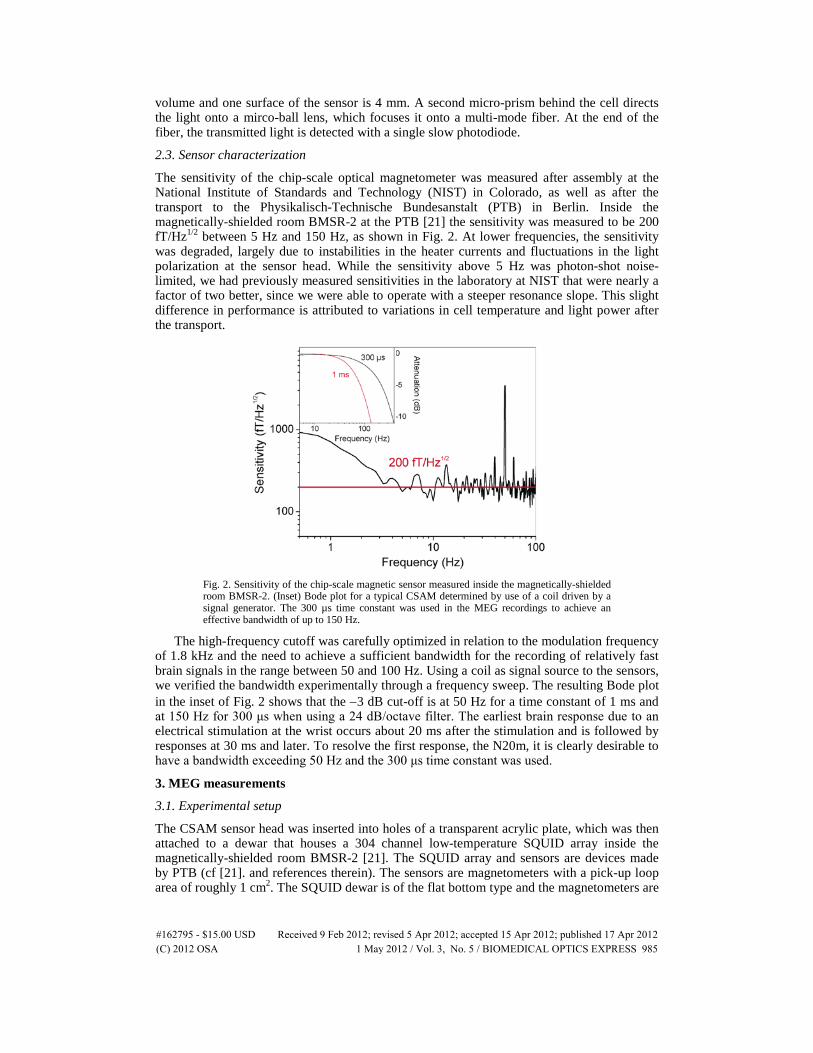
The sensitivity of the chip-scale optical magnetometer was measured after assembly at the National Institute of Standards and Technology (NIST) in Colorado, as well as after the transport to the Physikalisch-Technische Bundesanstalt (PTB) in Berlin. Inside the magnetically-shielded room BMSR-2 at the PTB [21] the sensitivity was measured to be 200 fT/Hz1/2 between 5 Hz and 150 Hz, as shown in Fig. 2. At lower frequencies, the sensitivity was degraded, largely due to instabilities in the heater currents and fluctuations in the light polarization at the sensor head. While the sensitivity above 5 Hz was photon-shot noise-limited, we had previously measured sensitivities in the laboratory at NIST that were nearly a factor of two better, since we were able to operate with a steeper resonance slope. This slight difference in performance is attributed to variations in cell temperature and light power after the transport.

Fig. 2. Sensitivity of the chip-scale magnetic sensor measured inside the magnetically-shielded room BMSR-2. (Inset) Bode plot for a typical CSAM determined by use of a coil driven by a signal generator. The 300 µs time constant was used in the MEG recordings to achieve an effective bandwidth of up to 150 Hz.

The high-frequency cutoff was carefully optimized in relation to the modulation frequency of 1.8 kHz and the need to achieve a sufficient bandwidth for the recording of relatively fast brain signals in the range between 50 and 100 Hz. Using a coil as signal source to the sensors, we verified the bandwidth experimentally through a frequency sweep. The resulting Bode plot in the inset of Fig. 2 shows that the −3 dB cut-off is at 50 Hz for a time constant of 1 ms and at 150 Hz for 300 μs when using a 24 dB/octave filter. The earliest brain response due to an electrical stimulation at the wrist occurs about 20 ms after the stimulation and is followed by responses at 30 ms and later. To resolve the first response, the N20m, it is clearly desirable to have a bandwidth exceeding 50 Hz and the 300 μs time constant was used.

3. MEG measurements

3.1. Experimental setup

The CSAM sensor head was inserted into holes of a transparent acrylic plate, which was then attached to a dewar that houses a 304 channel low-temperature SQUID array inside the magnetically-shielded room BMSR-2 [21]. The SQUID array and sensors are devices made by PTB (cf [21]. and references therein). The sensors are magnetometers with a pick-up loop area of roughly 1 cm2. The SQUID dewar is of the flat bottom type and the magnetometers are


sensitive to the normal direction of the bottom. The SQUID dewar was hanging vertically from the ceiling with the CSAM attached to the bottom center and therefore SQUIDs and CSAM measure the same field component, although there is a vertical offset between the two due to the vacuum space of the Dewar. The control system was kept outside the seven-layer mu-metal room, and the cables and fiber connections to the sensor head were routed through small tubes that penetrate the walls of the shielded room. The sensor was oriented such that the radial component of the magnetic field of the head was measured. Both CSAM and SQUID signals were collected with the same data recording system with a sampling rate of 1 kHz and an analog bandpass filter of 0.1 to 500 Hz. For the SQUID signals, the bandwidth given by the recording bandpass filter, while the bandwidth of the CSAM signals is limited by its driving circuitry, as was discussed in section 2.3.

Fig. 3. Sketch of the measurement positions on the head used to detect magnetoencephalographic signals. Spontaneous activity around 10 Hz linked to closing and opening of the eyes was measured with the sensor positioned above O1 (international 10-20 system for electrode positioning), whereas signals related to an electrical stimulation at the wrist were obtained over position C3.

3.2. Spontaneous brain activity

Spontaneous α–oscillations, triggered by a closing of the eyes, are employed in numerous studies as exemplary signals of spontaneous brain activity. The corresponding MEG was recorded for the first time several decades ago even before the advent of SQUIDs [22].

To detect α–oscillations, the magnetic sensors were placed over the occipital region of a subject (O1), the area where the signals were expected to be biggest (see Fig. 3). Here, both CSAM and SQUID array were positioned over the same area of the head, with the Dewar

Fig. 4. Time-frequency analysis of the CSAM signal (left) and a SQUID signal (right) obtained during a repeated sequence of 20 s of eyes open followed by 20 s of eyes closed. The eyes-closed sections start at 20 s and 60 s, lasting for 20 s as indicated, and the increase in α–power in the 10 Hz band is immediately visible both in the CSAM and the SQUID signal. Measurement position was O1, as sketched in Fig. 3 (International 10-20 system).


housing the SQUIDs above the CSAM at a much larger distance to the subject’s head. The subject was instructed verbally via a speaker to alternately close and open the eyes in intervals of 20 s. The alternating states of the eyes are known to induce changes of bioelectric brain activity in the alpha band (8-13 Hz) and, accordingly, should lead to related changes in MEG signal power around 10 Hz. To analyze the spectral content of the data, a wavelet transform (Morlet type) with a frequency resolution of 2 Hz was applied to the data. The results are shown in Fig. 4 as a time-frequency distribution of the CSAM time series (left) and a SQUID signal (right). The first twenty seconds refer to the condition with eyes open, and, upon closing the eyes at t = 20 s, signal energy clearly appears in the 10 Hz band for the next 20 s. This is repeated subsequently at 60 s. The two data sets for CSAM and SQUID were measured consecutively, without the subject changing positions. Simultaneous measurements were not possible, since CSAM heaters caused a perturbing field at 30 kHz that saturated the SQUIDs. The data of Fig. 4 give clear evidence for the detection of α–oscillations by the CSAM. The signal strength in the CSAM measurements is higher, due to a closer proximity of the CSAMs to the skull. We will come back to this point in the following section.

3.3. Somatosensory evoked fields (SEFs)

For applications such as studies on cognitive processes or clinical preoperative function mapping [23–25], brain responses due to a stimulation are often more important than spontaneous signals. A continuous signal is recorded for a sequence of up to several thousands of stimulations, and a stimulus-triggered average of the brain signal is calculated offline. This so called event-related field due to brain activity is usually completely obscured by technical noise in the raw data, biological artifact signals, and spontaneous brain signals unrelated to the stimulation. Here, we use an electrical stimulation at the wrist to evoke a well-defined biomagnetic brain activity starting 20 ms after the stimulus. This somatosensory-evoked field component, the N20m, is known since long from MEG studies using SQUIDs [26,27]. Here, we use CSAMs to measure N20m signals and compare them with those obtained with SQUIDs.

The dewar with the CSAM was placed roughly 5 mm from the scalp, above position C3 of a healthy human subject, lying on his right side, as sketched in Fig. 3. A 100 μs current pulse of 8 mA, repeated every 223 ms, was applied to the Median nerve of the right hand, which excites primarily the left somatosensory cortex associated with C3. In total, the MEG signal following the stimulation pulses was recorded sequentially using CSAM and SQUID, but without changing the position of the subject. The responses to the 5000 stimuli were averaged in the subsequent preprocessing of the data. It is known that the N20m response does not show habituation effects for at least 10000 stimulations [28] and the sequential measurement is a reasonable approach. By choosing a stimulation periodicity of 223 ms, any harmonic relation to the 50 Hz power-line noise is avoided. This means that the 50 Hz power-line noise is effectively suppressed in the averaged data and the N20m is clearly visible.

Averaged SEFs from recordings of three subjects (S1, S2, and S3) are shown in Fig. 5. For display purposes the SQUID signal was low pass filtered to achieve a bandwidth similar to the CSAM. Both CSAM and SQUID signal consist of a sequence of three peak regions. The first peak at 0 ms has a technical origin, because the current stimulation pulse at the wrist creates a magnetic field and the occurrence of this peak is indirect proof for proper recording conditions. The second peak can occur between 20 and 25 ms and it is of physiological origin. It is due to a focal current within the so-called somatosensory cortex, which becomes excited once the peripheral nerve signal is relayed through subcortical structures to the cortex. Note that the 20 ms delay between stimulation and brain response corresponds to the speed of signal propagation along the nerves, which is in the range of 50 m/s. The temporal location of the third peak is less well defined as several brain areas become activated in sequence after the N20m. The observed peak at about 50 ms (termed the P50m due to EEG nomenclature) is a superposition of contributions from more than one activity center [27], which can vary between subjects. Therefore a sequence of three peaks leads to the conclusion that the N20m is indeed observed in the CSAM signal in Fig. 5 of the three subjects.


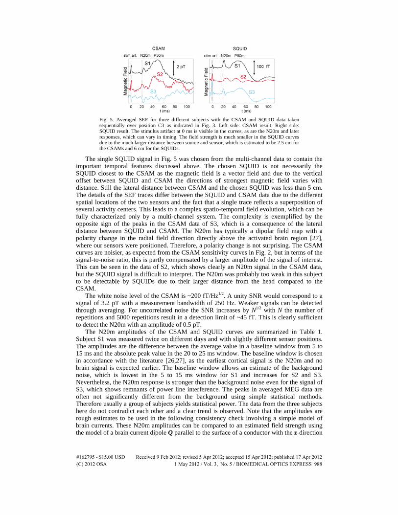
Fig. 5. Averaged SEF for three different subjects with the CSAM and SQUID data taken sequentially over position C3 as indicated in Fig. 3. Left side: CSAM result; Right side: SQUID result. The stimulus artifact at 0 ms is visible in the curves, as are the N20m and later responses, which can vary in timing. The field strength is much smaller in the SQUID curves due to the much larger distance between source and sensor, which is estimated to be 2.5 cm for the CSAMs and 6 cm for the SQUIDs.

The single SQUID signal in Fig. 5 was chosen from the multi-channel data to contain the important temporal features discussed above. The chosen SQUID is not necessarily the SQUID closest to the CSAM as the magnetic field is a vector field and due to the vertical offset between SQUID and CSAM the directions of strongest magnetic field varies with distance. Still the lateral distance between CSAM and the chosen SQUID was less than 5 cm. The details of the SEF traces differ between the SQUID and CSAM data due to the different spatial locations of the two sensors and the fact that a single trace reflects a superposition of several activity centers. This leads to a complex spatio-temporal field evolution, which can be fully characterized only by a multi-channel system. The complexity is exemplified by the opposite sign of the peaks in the CSAM data of S3, which is a consequence of the lateral distance between SQUID and CSAM. The N20m has typically a dipolar field map with a polarity change in the radial field direction directly above the activated brain region [27], where our sensors were positioned. Therefore, a polarity change is not surprising. The CSAM curves are noisier, as expected from the CSAM sensitivity curves in Fig. 2, but in terms of the signal-to-noise ratio, this is partly compensated by a larger amplitude of the signal of interest. This can be seen in the data of S2, which shows clearly an N20m signal in the CSAM data, but the SQUID signal is difficult to interpret. The N20m was probably too weak in this subject to be detectable by SQUIDs due to their larger distance from the head compared to the CSAM.

The white noise level of the CSAM is ~200 fT/Hz1/2. A unity SNR would correspond to a signal of 3.2 pT with a measurement bandwidth of 250 Hz. Weaker signals can be detected through averaging. For uncorrelated noise the SNR increases by N1/2 with N the number of repetitions and 5000 repetitions result in a detection limit of ~45 fT. This is clearly sufficient to detect the N20m with an amplitude of 0.5 pT.

The N20m amplitudes of the CSAM and SQUID curves are summarized in Table 1. Subject S1 was measured twice on different days and with slightly different sensor positions. The amplitudes are the difference between the average value in a baseline window from 5 to 15 ms and the absolute peak value in the 20 to 25 ms window. The baseline window is chosen in accordance with the literature [26,27], as the earliest cortical signal is the N20m and no brain signal is expected earlier. The baseline window allows an estimate of the background noise, which is lowest in the 5 to 15 ms window for S1 and increases for S2 and S3. Nevertheless, the N20m response is stronger than the background noise even for the signal of S3, which shows remnants of power line interference. The peaks in averaged MEG data are often not significantly different from the background using simple statistical methods. Therefore usually a group of subjects yields statistical power. The data from the three subjects here do not contradict each other and a clear trend is observed. Note that the amplitudes are rough estimates to be used in the following consistency check involving a simple model of brain currents. These N20m amplitudes can be compared to an estimated field strength using the model of a brain current dipole Q parallel to the surface of a conductor with the z-direction


normal to the surface (Eq. (35) in [1]). By applying this model we treat the head surface locally as a plane, which is sufficient to get an estimate of brain currents close to a sensor. The choice of a current dipole parallel to the plane reflects the fact that in a precisely spherical conductor geometry, only tangential currents contribute to the magnetic field. Following [1] the field Bz normal to the plane is

03

( ) .4

Q zz

Q

Q r r eBr r

µπ

× − ⋅=

−

(1)

Here r is the position of the sensor, rQ is the position of the current dipole, Q is the current dipole source, ez is the unit vector normal to the surface, and μ0 is the Bohr magneton. It is assumed for simplicity that Q and (r-rQ) are perpendicular to each other and that the CSAM and the SQUID are offset horizontally with respect to the position of the current dipole. Directly above Q the nominator in Eq. (1) is zero, and consequently Bz = 0.

Fig. 6. Sketch of the geometry of brain current dipole source Q parallel to the surface of a horizontally layered conductor and the two sensors used in this study. Both sensors measure Bz, which is zero directly above Q, and therefore the sensors are assumed to be offset horizontally.

This geometry is sketched in Fig. 6, and Eq. (1) simplifies to

03

sin( ),

4

Q

zQ

Q r rB

r r

αµπ

⋅ − ⋅=

−

(2)

where α is determined by the horizontal offset. In the literature [2,26] the magnitude Q for a somatosensory source is in the range of 10 nA m. Using this value for Q and a horizontal distance between rQ and sensors of 1 cm, a vertical distance between CSAM and rQ of 2.5 cm, and vertical distance between SQUID and rQ of 6 cm, the following results are estimated: Bz(CSAM) = 550 fT, Bz(SQUID) = 42 fT. This agrees well with observed values given in Table 1.

Table 1. Measured N20m amplitudes for CSAM and SQUID from the curves in Fig. 5

CSAM N20m (fT) SQUID N20m (fT)

S1 500 30 S2 700 20 S3 700 45 S1 700 50


4. Summary and outlook

We report on MEG measurements of healthy human subjects with a fiber-coupled chip-scale atomic magnetometer. Spontaneous and somatosensory-evoked brain fields were measured and validated with SQUID measurements. While the noise of the optical magnetometer was higher than that of the SQUID, this was partly compensated for by an increased amplitude of the physiologic signal of interest. This benefit was made possible by the small size of the CSAM and the easy handling of the devices, which enables the attachment of the sensors close to the surface of the skull, almost like conventional EEG electrodes.

The sensitivity of the CSAM sensor is currently limited by the photon-shot noise in the detected light. Since the beam diameter covers only 20% of the vapor cell area, and the detection efficiency is only 30%, the sensitivity of the CSAMs could be improved by an order of magnitude when more light is detected. More detailed numerical calculations suggest that sensitivities around 3 fT/Hz1/2 should be achievable with the current method [29]. Higher sensitivities can be reached with larger cell sizes, but since the noise floor in most commercially-available shielded rooms is of similar sensitivity, cell sized around (2 mm)3 seem reasonable. We furthermore plan to optically heat the CSAMs, which would eliminate the fields generated at 30 kHz and allow for simultaneous measurements with SQUIDs and CSAMs [30].

While these measurements presented here can give us some ideas about the capabilities of CSAMs as inexpensive, uncooled sensors for biomedical applications, the next step would be the design of a multi-channel system to be able to localize sources and to suppress noise signals using multivariate statistics such as principal component analysis (PCA) and independent component analysis (ICA). The spatial sampling needed for brain magnetic fields was analyzed for SQUID-based sensor arrays in [31]. Those results might need minor adjustments due to the smaller distance between brain source and CSAM compared to the brain to SQUID array geometry. Newer results [32] estimating the necessary number of sensors from the degrees of freedom of brain magnetic fields indicate that 100 sensors are the absolute minimum. Therefore, the optimal number of channels in a CSAM system is not obvious at present and will be investigated in the future. Further CSAM system design improvements might include closed-loop configuration to extend the dynamic range needed for less-well shielded environments, the demonstration of gradiometers, and full vector-field measurements. These might allow at some point a fully geometrically flexible and lightweight MEG system, although the reality of this is still a long way ahead. Many small developments are needed, e.g., the projection vectors for the subtraction of background noise cannot be easily computed for a flexible geometry.

Acknowledgments

All measurements on human subjects were carried out at the Physikalisch-Technische Bundesanstalt and followed established PTB IRB protocols for measurements of human subjects. This work is a contribution of NIST, an agency of the U.S. government, and is not subject to copyright. The measurements were performed collaboratively by J. P. and T. S and both authors have contributed equally to this work.


magnetoencephalography with a chip-scale atomic magnetometer

Documents