McGraw Hill 14th Edition

Standard Handbook for Electrical Engineers 1998

MAGNETOHYDRODYNAMICS

by M. S. Tillack and N. B. Morley

The authors wish to acknowledge the generous extraction of material on gaseous

MHD power generation from the previous edition, authored by John C. Cutting.

Contents

1. Introduction

2. Basic Equations

2.1 The Full Set of MHD Equations

The MHD equations

Magnetic induction

Dimensionless parameters

2.2 Electrical Equations and Ohm's Law

The Lorentz force

The Hall effect

Generalized Ohms Law

Circuits with conducting ducts

2.3 Basic Flow Characteristics and Power Production

Hartmann flow

Channel power and conversion efficiency

3. Liquid MHD

3.1 Introduction

3.2 Closed Channel Flows

3.2.1 Fully Developed Channel Flow

Equations and boundary conditions for 2D fully-developed flow

Invicid core flow and boundary layers

3.2.2 Developing flows, variable fields, variable duct sizes and

entrance effects

Duct flows in varying magnetic fields

General core flow equations

3.3 EM Pumps and Flow Meters

3.3.1 MHD flow meters

3.3.2 Conduction pumps

3.3.3 Induction pumps

3.3.4 MHD ship propulsion

3.4 Turbulence in Liquid MHD Flow

3.5 Open Channel Flows

Applications in metals processing

4. Gaseous MHD

4.1 Introduction

4.2 Generator Configurations

4.3 Energy Extraction and Flow Relations

4.4 Working Fluid Conductivity

5. Two-phase MHD

5.1 Flow characteristics

5.2 MHD generators and power conversion

1. Introduction

The interaction of moving conducting fluids with electric and magnetic fields provides for a

rich variety of phenomena associated with electro-fluid-mechanical energy conversion.

Effects from such interactions can be observed in liquids, gases, two-phase mixtures, or

plasmas. Numerous scientific and technical applications exist, such as heating and flow

control in metals processing, power generation from two-phase mixtures or seeded high-

temperature gases, magnetic confinement of high-temperature plasmas — even dynamos

that create magnetic fields in planetary bodies. Several terms have been applied to the

broad field of electromagnetic effects in conducting fluids, such as magneto-fluid-

mechanics, magneto-gas-dynamics, and the more common one used here — magneto-

hydrodynamics, or “MHD”.

Practical MHD devices have been in use since the early part of the 20th century. For

example, an MHD pump prototype was built as early as 1907 [1]. More recently, MHD

devices have been used for stirring, levitating, and otherwise controlling flows of liquid

metals for metallurgical processing and other applications [2]. Gas-phase MHD is prob-

ably best known in MHD power generation. Since 1959 [3,4], major efforts have been

carried out around the world to develop this technology in order to improve electric

conversion efficiency, increase reliability by eliminating moving parts, and reduce emis-

sions from coal and gas plants. Closed-cycle liquid metal MHD systems using both single-

phase and two-phase flows also have been explored.

Still more novel applications are in development or on the horizon. For example, recent

research has shown the possibility of seawater propulsion using MHD [5] and control of

turbulent boundary layers to reduce drag [6]. Extensive worldwide research on magnetic

confinement of plasmas has led to attainment of conditions approaching those needed to

sustain fusion reactions [7].

In the following sections, we review the basic equations describing coupled MHD behavior

as well as some basic MHD phenomena in liquids, gases and two-phase mixtures. Much

of the underlying physics described is common to many of the applications cited above.

Also included are discussions of several of the most important applications, together with

their special analysis techniques and examples of equipment involved.

2. Basic Equations

2.1 The Full Set of MHD Equations

The MHD Equations

The complete set of magnetohydrodynamic equations for a Newtonian, constant property

fluid flow includes the Navier-Stokes equations of motion (i.e., momentum equation), the

equation of mass continuity, Maxwell’s equations, and Ohm’s Law. In differential form

they constitute the following system of equations:

u

t + (u• )u = – p + j B + f 2u + g (1)

/ t + • u = 0 (2)

E = – Bt (3)

B = m j (4)

j = (E + u B) (5)

where the MHD body force j B is included in the Navier-Stokes equation The displace-

ment current has been neglected from Ampere’s Law, which is a valid approximation for

non-relativistic phenomena typical of the response of an inertial liquid. Implicit in Eqs.

1–5 are the following additional relations:

• B = 0 (6)

• j = 0 (7)

This system of equations is a rich one, describing not only all of the phenomena generally

associated with electromagnetics and fluid mechanics, but new phenomena not seen in

either discipline. Simplifications usually are required to obtain solutions to physical sys-

tems of interest. For instance, for quasi-steady flow problems where t is negligible,

the electric field can be represented as the gradient of an electric potential , which simpli-

fies the problem by eliminating vector Eq. 3.

Magnetic induction

The magnetic induction equation is derived easily by taking the curl of Ohm's Law:

j/ = E + u B) (8)

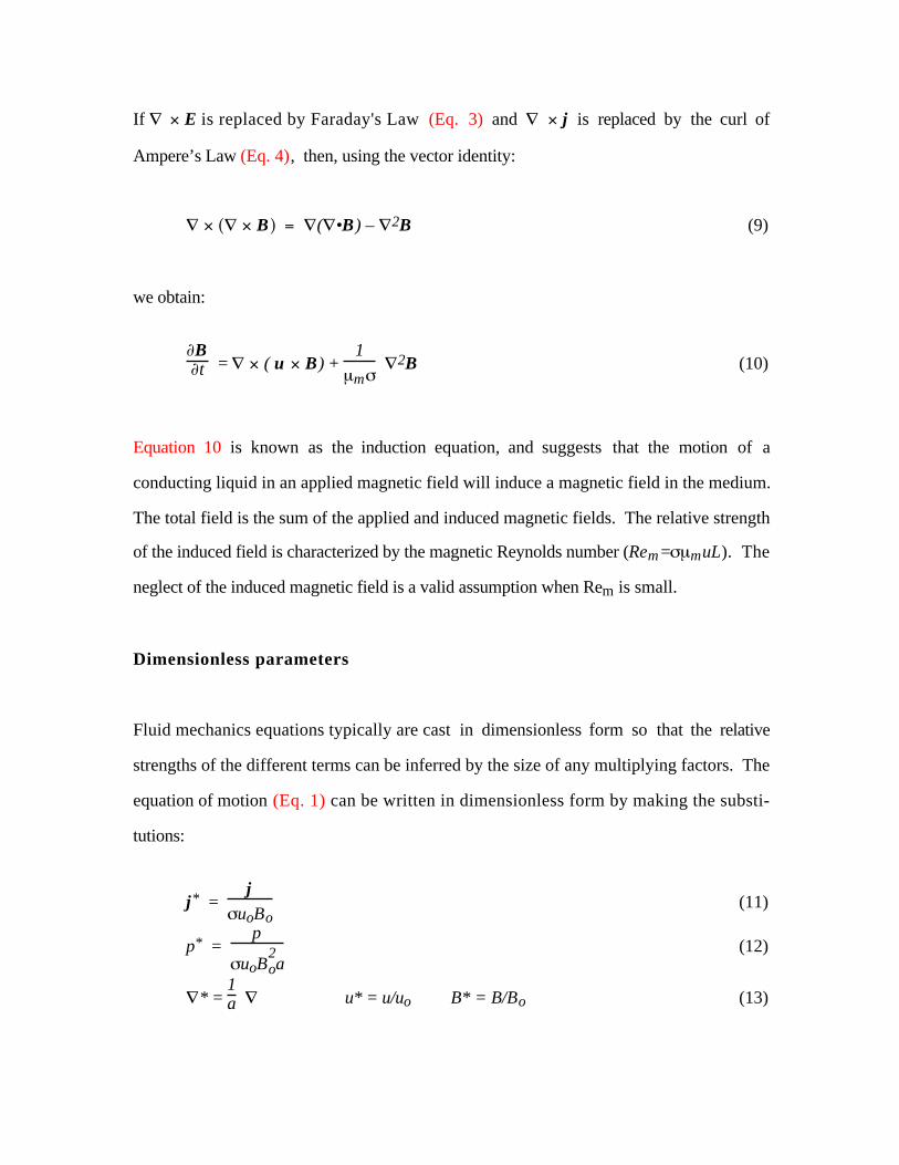
If E is replaced by Faraday's Law (Eq. 3) and j is replaced by the curl of

Ampere’s Law (Eq. 4), then, using the vector identity:

B ( •B) – 2B (9)

we obtain:

Bt = ( u B) +

1

m 2B (10)

Equation 10 is known as the induction equation, and suggests that the motion of a

conducting liquid in an applied magnetic field will induce a magnetic field in the medium.

The total field is the sum of the applied and induced magnetic fields. The relative strength

of the induced field is characterized by the magnetic Reynolds number (Rem= muL). The

neglect of the induced magnetic field is a valid assumption when Rem is small.

Dimensionless parameters

Fluid mechanics equations typically are cast in dimensionless form so that the relative

strengths of the different terms can be inferred by the size of any multiplying factors. The

equation of motion (Eq. 1) can be written in dimensionless form by making the substi-

tutions:

j* = j

uoBo (11)

p* = p

uoB2oa

(12)

* = 1a u* = u/uo B* = B/Bo (13)

where a, uo and Bo are characteristic values of length, velocity and applied magnetic field.

Characteristic values of the current density and pressure have been selected carefully in

order to scale the phenomena of interest; different values could have been selected, leading

to different systems of non-dimensionalization. Using this system, the equation of motion

(excluding gravity) becomes:

1N

u*

t + (u*• )u* = – p* + j* B* +

1Ha2 2u* (14)

The characteristic parameters Re, Ha and N are the Reynolds number, the Hartmann

number, which is an average measure of the ratio of magnetic to viscous forces, and the

interaction parameter, which is a measure of the ratio of magnetic to inertial forces. They

are defined as:

Re = uoa/ f (15)

Ha = aBo f / f (16)

N = Ha2/Re = aB2o f / uo (17)

Table 1 gives representative values of these characteristic dimensionless parameters for

example cases of interest. When the Hartmann number and interaction parameter are both

sufficiently large, the momentum equation (Eq. 14) throughout the bulk of the fluid can be

reduced to the simple form:

p = j B (18)

2.2 Electrical Equations and Ohm's Law

The Lorentz force

Underlying the MHD body force is the fact that free charges moving in a magnetic field

experience a “Lorentz” force perpendicular to both their velocity and the magnetic field

induction:

Fq = q (v B) (19)

For collisionless particles, the Lorentz force results in pure harmonic motions in the plane

perpendicular to the magnetic field (Bz) with characteristic cyclotron frequency c=qBz/m:

m •vy = – q vx Bz m •vx = q vy Bz (20)

••vy = –qBzm •vx = –

qBz

m 2 vy

••vx = qBzm •vy = –

qBz

m 2 vx (21)

vy = A1 cos ωct + A2 sin ωct vx = A3 cos ωct + A4 sin ωct (22)

In contrast, for collisional particles that are forced to follow the fluid velocity u, the Lorentz

force acts on electrons and ions in a direction perpendicular to the flow, but in in opposite

directions for positive and negative charges. The net result is charge separation, leading to

electric fields. The open circuit voltage between electrodes spaced a distance d apart in a

conducting fluid is:

Voc = ⌡⌠o

d

( u B) • d l (23)

An electric field arises between the electrodes such that +u B=0, corresponding to the

zero-current condition in Ohm’s Law (Eq. 5). If current is allowed as a result of some

return current path, then the electric field and electrode voltage are reduced due to the

electrical resistance of the fluid:

= (u B – j/ ) (24)

The Hall effect

In the regime between collisional and collisionless particles, the Hall effect can be impor-

tant. Usually the current induced in the fluid is carried predominantly by electrons, which

are considerably more mobile than ions. The electron drift velocity, given by:

j = nee ue (25)

leads to a second component of velocity, and so, according to Eq. 19, a secondary force

and electric field:

H = j B (26)

where β=1/nee is the Hall constant. The current component created by this electric field,

i.e. the “Hall current”, is given by – ej B , where e= /B is the electron mobility. This

leads to a more generalized statement of Ohm’s Law including the Hall effect:

j/ = ( + u B) – e j B (27)

A vector diagram of the electric field components from this relation is shown in Fig. 1.

Further theoretical discussion of the generalized Ohm's Law can be found in Refs. 8–11.

Generalized Ohm's Law

Ohm's Law cited above is a constitutive relationship (for instance, analogous to the

equation of state for gases) and as such has a limited range of applicability. Various forms

of Ohm’s Law can be obtained depending upon the approximations made in deriving the

current-field relationships from the equations of motion and the interactions of the

constituent parts of the fluid. For weakly-ionized gases in thermal equilibrium at moderate

temperature, Eq. 27 has the equivalent tensor form (neglecting ion current):

j = ^ • ( + u B) = ^ • * (28)

or

j = k

k

*k (29)

When B = z1 Bz,

^ / f =

1

1 + 2 2

–

1 + 2 2 0

1 + 2 2

1

1 + 2 2 0

0 0 1

(30)

where

= eBme

electron cyclotron frequency

= ce electron collision mean free time

= eB Hall parameter

The dimensionless product , often called the “Hall parameter”, is an important

characteristic number in MHD design. The conductivity tensor is anisotropic due to the

Hall component unless ωτ«1 (typical values for weakly-ionized gases are 1–5). On a

microscopic scale, the Hall parameter indicates the average angular travel of electrons

between collisions. Typical values are ~10–7 m, ce~105 m/s, ~10–12 s,

x ~ 1012 /s for B=6 T. Since the mean free path is inversely proportional to

pressure, lower pressure and higher values of B give larger values of ωτ.

On a macroscopic scale, the value of indicates the relative importance of the Hall field

and Hall current. When =1, the total current is directed 45˚ to the left of the ε* vector

(see Figure 1), and for large values of the current vector is nearly perpendicular to ε*

(predominantly Hall current). In weakly-ionized gases, if both the electron ( ) and ion

( i i) Hall parameters are large simulataneously then the angle is reduced. In this case, the

conductivity is reduced due to a phenomenon called “ion slip”. Even though i is ordinarily

larger than e, i is much smaller than e, such that the product i i is usually negligible.

For highly collisional fluids (such as condensed liquids) where τ→0, the Hall current is

negligible, and the use of Eq. 5 without further modification is satisfactory.

Circuits with conducting ducts

For MHD flows in electrically conducting ducts with no external load, a return current can

exist in the duct walls (see Fig. 2). For a uniform flow velocity u, the loop voltage

equation is written:

o∫ • dl = 2b

uB – jy

f – 2b

jw

w = 0 (31)

where the subscript w denotes values in the wall. Conservation of current dictates:

jy a = jw (32)

so that Eq. 31 becomes:

jy = f uB (33)

where Φ is the “wall conductance ratio”:

= w

fa (34)

For this type of uniform flow, Eq. 18 can be used to estimate the pressure required to drive

a flow at velocity u through the duct.

2.3 Basic Flow Characteristics and Power Production

Hartmann flow

Equation 33 predicts zero current when the walls are not electrically conducting, however,

the no-slip condition on the fluid at the walls results in a non-uniform channel velocity and

the formation of a boundary layer with a reduced u B emf, allowing a conducting return-

current path through the fluid itself.

For 1-D, fully-developed (hence inertialess) flow, the momentum equation for ux(z)

becomes:

dpdx = jy Bz + f

d2ux

dz2 (35)

where dpdx is constant, and Ohm’s Law is:

jy = ( – ux Bz) (36)

The electric field also is constant. Substituting Ohm’s Law into the momentum equation,

we obtain a simple differential equation for ux:

fd2ux

dz2 – fB2ux =

dp

dx – fB (37)

The solution to this equation is:

uxub

= Ha cosh Ha

Ha cosh Ha – sinh Ha

1 – cosh Ha

za

cosh Ha (38)

where ub is the bulk average velocity. For large values of the Hartmann number, Eq. 38

simplifies to:

uxub

1 – exp

Ha

z

a – 1 (39)

Equation 39 describes a velocity profile that is nearly flat throughout the duct, with thin

boundary layers at the walls where viscous drag forces the flow to zero. The thickness of

the Hartmann boundary layer scales as a/Ha. The shape of the Hartmann profile is shown

in Fig. 3 for a range of Hartmann numbers.

Channel power and conversion efficiency

The total electric power generated internally in a channel is equal to the mechanical work

against the MHD body force, which is given by the product of the volume flow rate and

pressure drop.

For a distributed medium, the Lorentz force leads to the pressure gradient:

p = nFq = nqv B = j B (40)

so that the power density is simply:

Pi = u • p = u • (j B) (41)

The amount of power delivered to the external load is

PL = j • (42)

so that we can write the local electrical efficiency as:

e = PiPL

= j•

ux jy B z (43)

3. Liquid MHD

3.1 Introduction

As seen above, the presence of the j B force on the flow of conducting liquids can alter

the velocity and pressure characteristics of the flow. The interaction with a magnetic field

also can significantly delay the onset of turbulent fluctuations. These two effects together

or individually can dramatically alter the heat transfer characteristics and fluid drag in closed

or open channel flows. Technological applications of such phenomena include cooling

systems for magnetic fusion reactors and reduced-drag ship hulls and airplane fuselages.

The MHD force can be applied in such a way that useful work can be done. For example,

EM pumps can be designed to precisely control liquid flows – liquid metal flows, in

particular – where high temperature and corrosive tendencies prohibit the use of seals in

standard mechanical pumps. Such pumps have no moving parts and are extremely reliable.

The converse is also possible; MHD generators can produce high currents at low voltages.

This section is concerned with exploring the interaction of the magnetic field with liquid

flows both with and without applied electrical currents. For incompressible liquids, the

equations of Section 2.1 are valid, with Eq. 2 reduced to:

•u = 0 (44)

A discussion of various applications where such phenomena are encountered is included as

well. More comprehensive discussions of many of these subjects can be found in text-

books [12–14] as well as the numerous other references provided throughout this section.

3.2 Closed Channel Flows

3.2.1 Fully Developed Channel Flow

The term fully developed, used to describe Hartmann flow in Section 2, denotes a

condition where the velocity profile is no longer changing (zero derivative) in the main flow

direction, i.e., a flow that has reached a stable steady state driven by a constant pressure

gradient, P = –dp/dx. The study of fully-developed flow with a constant applied magnetic

field is useful because the equations can be solved analytically for a variety of cases, and

then can be used as benchmark problems for complete numerical algorithms. In addition,

the fully developed solutions predict some phenomena of general interest, especially the

existence of different boundary layers, which are important for a general understanding of

MHD flows. By controlling the amount of current that can flow in the main body of the

liquid, these boundary layers and the MHD boundary conditions exert a significant

influence on the velocity profile and pressure drop.

Equations and boundary conditions for 2D fully-developed flow

In a rectangular channel (a round pipe is fundamentally the same), we denote the flow

direction as x and restrict the applied magnetic field Bo to be constant and aligned with z, as

seen in Fig. 2. The MHD equations, Eqs. 1, 3–5 and 44, can be simplified to the

following form:

f

2u

y2 + 2uz2 +

Bo

m

Bz = –P (45)

1

f m

2B

y2 + 2Bz2 + Bo

uz = 0 (46)

where the velocity vector has only one component in the x-direction, and the magnetic field

is the sum of the constant applied field in the z-direction and the small field induced in the x

direction.

u = [u(y,z),0,0] B = [B(y,z),0,Bo] (47)

Terms quadratic in Bx have been discarded as small, an assumption equivalent to assuming

small Rem, so that B really represents a stream function for the electric current, where:

mjy Bx/ x mjz – Bx/ z (48)

Walls parallel to the magnetic field (i.e., “side walls”) are located at y = ±b, and walls

perpendicular to the field (i.e., “Hartmann walls”) are located at z = ±a. The boundary

condition for the velocity is the standard fluid-mechanical no-slip condition:

V = 0 (@ all walls). (49)

For certain boundary conditions on the induced field B, analytic solutions exist in the form

of infinite series to the system. Much of the classical work in the 1950’s and 1960’s

focused on solving these equations either exactly or approximately by expanding one

dimension in an appropriate set of eigenfunctions. Some boundary conditions for the

induced field are summarized in Eqs. 50–52. These conditions are derived by considering

the behavior of the normal n and tangential s current at the wall, and using Eq. 48 to phrase

these conditions in terms of the induced magnetic field.

B = 0 electrically insulated wall [15], [16] (50)∂B∂n = 0 perfectly conducting wall [17] (51)

aΦ∂B∂n – B = 0 thin conducting walls [18], [19], [20] (52)

Invicid core flow and boundary layers

When Ha is large, the infinite series solutions cited above show (see Fig. 4) the existence

of a flat, inviscid core region in the central section of the duct, bordered by different types

of viscous boundary layers near the Hartmann walls and side walls [21]. In this core

region, the driving force of pressure is balanced entirely by the MHD force, p = j B .

The curl of this equation implies (B )j = 0, indicating that the current density is constant

along (applied) field lines in the core. A constant pressure and a constant current produce a

flat constant velocity in the core region.

On the Hartmann walls at z = ±1 , a Hartmann layer forms (similar to that seen in the 1D

example of Section 2.3), as shown in Figure 5 . Hartmann layers have thickness of a/Ha,

and join smoothly to the core value of the velocity. The Hartmann layer serves as a region

where electric currents induced in the core flow in the y-direction can return and complete

the current loop. This role as current return path makes the Hartmann layer an active

boundary layer, one whose properties controls the amount of flow possible in the core

region. If the Hartmann wall is electrically conducting, the electric current will flow

preferentially in the wall, and the influence of the Hartmann layer on the core flow will be

accordingly reduced.

In most cases, it is the combined conductivity of the Hartmann layer and Hartmann wall

that determines the MHD resistance to the fluid flow in the core, and so governs the

pressure gradient P (i.e., the pressure gradient required to drive the flow at a given average

velocity). In an electrically insulated channel, the increase in P is due to increased shear

friction at the walls as a result of the modification of the parabolic laminar velocity profile.

The average electromagnetic force in this case is zero since all the current induced in the

flow closes through boundary layers in the fluid itself. For large Ha, P increases linearly

with Ha. For electrically conducting channels, the net electromagnetic force is no longer

zero, but can in fact be quite large. For perfectly conducting channel with large Ha, P

increases with Ha2.

On the side walls at y = ± , one observes the formation of a different type of boundary

layer, alternately known as a “side layer”, “shear layer”, or “Shercliff layer”. The inter-

pretation of these layers is a region where mismatched electric potentials equalize, some-

times with a significant jet of liquid when the Hartmann walls are electrically conducting

(this is the case pictured in Fig. 4). These jets can carry an appreciable portion of the net

mass flux under certain cases. The thickness of side layers is of order a/Ha1/2, which is

much greater than that of the Hartmann layer. Thus, in most cases (except when the

Hartmann walls are highly conducting but the sidewalls are not), the electrical resistance of

the side layers does not add significantly to the total resistance of the return current path,

and so does not influence the core velocity. For larger Hartmann numbers on the order of

103 or 104, the flow in the core region drops almost to zero, and the velocity jets can be up

to a factor of Ha times the core flow velocity. Obviously, such velocity structures can be

very important in determining heat transfer in liquid metal coolant pipes, as well as

affecting corrosion, mass diffusion and other important physical processes.

Hartmann layers will form on any wall that has a normal component of Bo, but shear layers

form only along the magnetic field lines. Thus, if the channel is not perfectly aligned with

Bo, then all walls will have Hartmann layers, and the shear layers will detach from the wall

and form about the magnetic field line that intersects the corner of the duct (see Fig. 5b).

Shear layers that extend into the fluid are known as free shear layers [22].

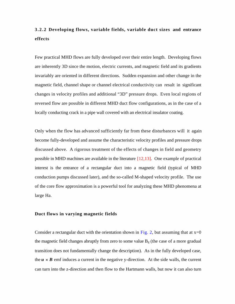
3 .2 .2 Developing flows, variable fields, variable duct sizes and entrance

effects

Few practical MHD flows are fully developed over their entire length. Developing flows

are inherently 3D since the motion, electric currents, and magnetic field and its gradients

invariably are oriented in different directions. Sudden expansion and other change in the

magnetic field, channel shape or channel electrical conductivity can result in significant

changes in velocity profiles and additional “3D” pressure drops. Even local regions of

reversed flow are possible in different MHD duct flow configurations, as in the case of a

locally conducting crack in a pipe wall covered with an electrical insulator coating.

Only when the flow has advanced sufficiently far from these disturbances will it again

become fully-developed and assume the characteristic velocity profiles and pressure drops

discussed above. A rigorous treatment of the effects of changes in field and geometry

possible in MHD machines are available in the literature [12,13]. One example of practical

interest is the entrance of a rectangular duct into a magnetic field (typical of MHD

conduction pumps discussed later), and the so-called M-shaped velocity profile. The use

of the core flow approximation is a powerful tool for analyzing these MHD phenomena at

large Ha.

Duct flows in varying magnetic fields

Consider a rectangular duct with the orientation shown in Fig. 2, but assuming that at x=0

the magnetic field changes abruptly from zero to some value Bz (the case of a more gradual

transition does not fundamentally change the description). As in the fully developed case,

the u B emf induces a current in the negative y-direction. At the side walls, the current

can turn into the z-direction and then flow to the Hartmann walls, but now it can also turn

(more easily) into the x-direction and return to the other side wall through the region of no

field directly adjacent to the region of high field, see Fig. 6. The same electric field set up

by the charge seperation that drives return current through the Hartmann layers (walls) will

drive this current in the no-field region. Thus, an additional current closure path exists,

and so more core current can flow in the high field region as compared to the correspon-

ding fully developed flow in a region of constant Bz. This additional current results in a

greater pressure drop, usually denoted ∆p3D.

The current in the x-direction near the side walls also causes a distortion of the velocity

profile near the region of changing Bz. The jx current, which is positive in the upper part

of the channel (y > 0), will induce a force in the negative y-direction near the sidewall.

This force will essentially pressurize the sidelayer, and cause a velocity jet to form in the

sidelayer. A similar result occurs in the lower half (y < 0) plane. The result is a velocity

profile called “M-shaped”, where the velocity is reduced in the core due to increased j B

forces, but increases in the side layers. This looks very similar to the side layer jets that

can occur in fully-developed flow when the Hartmann walls are electrically conducting, but

the M-shaped profile forms in the developing region even when the entire channel is non-

conducting. Like the fully-developed side layer jets, the M-shaped velocity profile is

shorted out when the side walls are highly conducting, since the jx current preferentially

flows in the walls in this case, and no force is induced in the liquid itself. The same effect

occurs at the exit of a magnetic field, and even if the field is more gradually varied.

Mathematically, the formation of the M-shaped velocity profile can be understood by taking

the curl of the steady invicid equation of motion:

(u• )u = – p + j B (53)

and considering the z component of vorticity:

u z

x – jx Bzx – Bz

jyy (54)

Both terms on the right hand side of Eq. 54 will be negative in the upper right quadrant of

Fig. 6, and positive in the lower right quadrant. These sources of z-directed vorticity can be

thought of as swirling motion around z that decelerates the center and shifts fluid to the side

layers causing the formation of the velocity jets. It is easily seen that the formation of side

layer jets in fully-developed flow is also governed by the last term in the above equation,

which is present in regions of constant Bz as well.

General core flow equations

For high conductivity liquids like liquid metals, calculations can become very difficult

unless simplifying approximations are made. One such approximation indicated by the

above discusion is the so called core flow approximation, where the momentum equation is

simplified to:

p = j B (55)

In 1968, Kulikovskii [23] showed that the core equations (Eqs. 5, 7, 44 and 60) could be

manipulated in such a way as to reduce the solution for any flow geometry without side

walls or internal shear layers to, at most, four two-dimensional partial differential

equations. In addition, the magnetic field is assumed to arise from external currents only

(Rem=0). The unique features of these equations allow us to separate components of

velocity and current into components parallel and perpendicular to the magnetic field:

J = BB2 p (56)

J|| = ⌡⌠

B

1B2 • p dl + A1 (57)

v = – 1

B2 p + BB2 (58)

v|| = ⌡⌠

B

1B2 • +

p •

1

B2 + 2p

B2 dl + A2 (59)

J⊥ is obtained by taking the cross product of B with the momentum equation (Eq. 55).

Similarly, v⊥ is obtained by taking the cross product of B with Ohm’s Law (Eq. 5). J||

and v|| are obtained by integrating the conservation laws (Eqs. 7 and 44) along the magnetic

field direction, dl, defined by ∇|| = ddl .

Finally, the electric potential can be related to the parallel current:

l = J|| (60)

= ⌡⌠

⌡⌠

B

1B2 • p dl´ dl + A1l + A3 (61)

The boundary conditions at the walls completely determine the unknown functions (A1,

A2, p, and φ). There are four boundary conditions. Zero mass flux into the walls and

conservation of current are applied twice for each field line: once where the field line enters

the fluid and once where it exits.

v • n = 0 (62)

= J • n for conducting ducts (63)1

Ha ( v ) • n = J • n for nonconducting ducts (64)

This method has been successfully applied to the solution of a number of basic geometries

[24]. For symmetric problems, the constants A1 and A2 can be eliminated. The constant

A3 can be replaced by the evaluation of ϕ at any location along l. (For example, A3 can be

replaced by ϕw – the potential at one wall.) In this case, only two partial differential

equations remain for p and ϕw.

The resulting set of linear partial differential equations can be solved using any appropriate

numerical technique. In the work described in [24], a finite difference representation was

applied and SOR was used to solve the resulting system of algebraic equations.

Corrections for side layers and internal shear layers also have been developed [25].

3.3 EM pumps and Flow Meters

One of the more practical uses of the MHD force is in pumping systems, where electrical

energy is converted directly into force on the working liquid. “EM pumps” (as they are

commonly known) have been in existence for many years, and many different designs have

been successfully developed and employed. A generic conduction style pump is shown in

Fig. 7. Another common MHD device is the EM flow meter, where the potential induced

by fluid motion is measured and used to infer the average flow rate

These devices can be constructed with no moving parts and no direct contact with the

working liquid. This is a distinct advantage if high temperature and/or corrosive liquids

must be handled. The absence of seals or moving parts leads to a highly reliable system.

In addition, EM pumps are typically controllable, and even reversible, by varying the

magnitude and direction of the applied current.

3 .3 .1 MHD flow meters

Eq. 23 suggests that the voltage induced by the u B emf would provide an ideal method

by which one could measure the average flowrate of a conducting liquid. However, it is

impossible to achieve a completely open-circuit configuration as described by Eq. 23, as

return current will flow in pipe walls and boundary layers of all finite size channels. Some

accounting for these return currents must be included when determining a relation for the

voltage signal as a function of the flow velocity. Ohm’s Law, as written in Eq. 24, shows

the effect of return currents on the measured voltage signal in a rectangular channel like that

in Fig. 2:

– /2b = uB – j/ (65)

where is the voltage signal. Any core current allowed to flow, then, reduces the

measured voltage signal by some amount. Using the result of Eq. 33 for the core current

density we see that the voltage signal is:

= 2buB

1+ =

QB

2a(1+ ) , (66)

which is independent of the electrical conductivity of the liquid, except as it appears in the

wall conductance ratio . This means that many moderately conducting liquids can also be

measured by this method, especially when an electrically insulated channel can be used (for

insulated channels, substitute Ha–1 for Φ in Eq. 66). For common laboratory and indus-

trial values of the flowrate Q, magnetic field induction and duct dimensions, the measured

voltage is typically in the range of hundreds of microvolts to several millivolts.

Most MHD flowmeters do not use rectangular channels, but instead use round pipes that

can fit easily into standard piping systems, like that shown in Fig. 8. Ref. [26] suggests

the following relation for the volumetric flowrate in a pipe made of an electrically conduc-

ting material:

Q = 3162 k4

k1 k2 k3 d

(67)

where Q is in units of gpm, B is in Gauss, the inside pipe diameter d is in inches and the

electric leads to measure are attached to the outside of the pipe wall.

Equation 71 takes into account, in the form of semi-empirical multiplicative constants k1-4,

several non-ideal effects that were ignored in Eq. 65. k1 is the pipe-wall current shunting

correction factor defined as:

k1 = 2dD

D2 + d2 + w

f ( )D2 – d 2

(68)

where D is the outside pipe diameter, also in inches.

Poorly conducting liquids tend to have a k1 correction factor that deviates significantly from

unity, meaning that the electrical signal is lower for the same flowrate and so more difficult

to measure accurately. k2 is the magnetic field end-effect correction factor. It is empirically

obtained as a function the magnet pole piece length L . Typical values are given in Table 2.

k3 is the magnetic material, temperature correction factor, which accounts for changes in the

magnetic field as a function of temperature of the permanent magnetic material or electro-

magnet windings. The manufacturer of such materials typically provides the appropriate

temperature correction factors. k4 is the pipe thermal expansion correction factor which

accounts for changing pipe sizes as a function of temperature, and can be expressed as k4 =

1 + (T – To), where γ is the thermal expansion coefficient for the pipe material. For 304

stainless steel the value of γ is 9.6 µ-in/in F

The idea behind these simple DC flowmeters has evolved into more complicated imple-

mentations where pulsed DC or pulsed AC electromagnets are used to sample the flowrate

at some pulse rate. The pulsed electromagnet devices have lower power consumption and

lower heat generation in the electric coils. These devices are available commercially [27]

with all manner of pipe materials and sizes, and can be inserted easily into existing piping

configurations. Small units (d ≈ 1 inch) have accuracies of around 1% at full scale. The

accuracy tends to improve as pipe sizes become larger.

3 .3 .2 Conduction pumps

Liquid metal conduction pumps, or “Faraday” pumps, consist of a rectangular channel in

the gap of a magnet (either a permanent or electromagnet) where an electric current is

passed through the conducting liquid perpendicular to the field. The resulting j B force

drives the flow. This type of pump is a conceptually simple extension of the rectangular

duct flows discussed above with side walls replaced by electric bus bars connected to an

outside voltage source which drives current in the direction opposite to the v B emf.

To understand the pressure and flow rate behavior of a simplified conduction pump,

pictured in Fig. 7, it is helpful to represent the pump by an equivalent electrical network

(Fig. 9). Here RLM is the effective resistance of the liquid in the channel, RLoss is the

resistance of any loss paths such as the channel walls and fringing paths outside of the

magnetic field area, and Ei is the voltage induced in the flow which works against the

applied current, Ia. Assuming slug flow of flow rate Q in a rectangular pumping channel of

flow length L within the field, with walls of thickness δw and electrical conductivity σw,

the following approximations can be applied:

RLM = b

La f RLoss =

b

L w w (69)

ILM = 2a p

B Ei = 2bvB = QB2a (70)

The duct geometry used is the same as in Fig. 2, and the RLoss term only takes into account

current losses through conducting Hartmann walls. The circuit then can be solved to give

the following linear relationship between pressure and flow rate:

∆p = BAIa/2a – B2LQΦσf

A(1+Φ) (71)

where A = 4ab is the flow cross sectional area, and Φ is the wall conductance ratio defined

in the usual way as in Eq. 34. This relationship is plotted in Fig. 10 for a small conduction

pump with various values of Φ. We see the obvious need for thin and/or low conductivity

walls in the pumping channel structure in order to maximize the pumping power. In the

case of Φ = 0.1, all of the applied current is simply shunted through the walls, as the

induced emf is larger than the applied voltage. Current flow in the core is reversed and

MHD drag, instead of pumping, results.

The applied voltage for this particular pump, assuming Q=10 l/s and Φ=0.01, is only 213

mV. The inherently low voltage and high current of conduction pumps is one of their

disadvantages, since they require special power supplies capable of coupling efficiently to

such a load. Possible power supplies which are more efficient than standard transformer-

rectifier systems include homopolar and unipolar generators, which can be up to 80%

efficient. To increase the voltage of the load somewhat, it is common to run the field coil

windings of the electromagnet in series with the LM section, so that only one supply (albeit

at a greater power level) is needed.

The power dissipated in the conduction pump system for our example above is:

Pa = 0.215 V • 1500 A = 322 W (72)

The power delivered to the fluid (Q • ∆p) is Pf = 0.01 m3/s • 25.7 kPa = 257 W. This

gives an efficiency of 81%. A formula for the electrical efficiency in the general case is

easily constructed in terms of either the applied voltage or the applied current:

e = Q pVaIa

= BQ

2aVa

1 + 1–BQ/2aVa

= 2bIa – BLQ f

2bIa

1 + 2bIa

BLQ f

(73)

However, the losses in the wall included in this simple calculation are not the only losses

the conduction pump experiences. Applied current usually fringes outside the area of the

applied magnetic field where it induces no j B force. Energy is lost to the damping of

turbulence and restructuring of the average velocity profile as the liquid enters the magnetic

field area. Energy losses occur due to friction of the flow on the channel walls and the

applied magnetic field is altered by the field induced by the applied current itself. All of

these effects decrease the net efficiency of conduction pumps to the order of 15–20% for

small pumps, and 40–50% percent for larger pumps. Including losses in generators and

field windings, the bus bar efficiency for liquid metal conduction pumps varies from 10%

to 40%, increasing with pump size [28].

As seen from Eq. 73, even in the absence of losses other than the resistance of the LM

itself, the electrical efficiency of the system is equal to ηe = ηind = 2bvB/Va, which is the

induction efficiency, i.e., the ratio of induced voltage due to the v B emf to the applied

voltage Va.

3 .3 .3 Induction Pumps

An alternative to the conduction pump is the induction pump, where electric currents are

induced in the liquid metal by means of a time-varying magnetic field, producing a j B

force with the instantaneous field to drive the flow. Many types of induction pumps are

possible. Here we focus on the flat linear induction pump and the annular linear induction

pump. The advantage of induction pumps is that they can be driven easily by single-phase

or 3-phase AC power sources, possibly with a step transformer for control of the flow rate.

Typical disadvantages are greater power losses and the need for electrical insulation at high

temperatures close to the working liquid.

The flat linear induction pump, or FLIP, is conceptually similar to an AC induction motor.

The 3-φ winding, however, produces a sliding, rather than rotating magnetic field, which

tends to pull the fluid along. The action of this class of pump is easily pictured by contem-

plating the simplified induction pump shown in Fig. 11. If the peak vertical magnetic field

is sliding to the right, leaving behind a slightly reduced magnetic field, a current loop will

be induced. This induced current tries to maintain the field at its original strength. The

induced current into the page will be in a region of stronger magnetic field than the current

coming out of the page, since the field peak is propagating to the right, so the net j B

force will to the right.

The disadvantage to these systems is that in order to have a relatively wide channel for

liquid flow, the gap between the stators must be larger than that in induction motors, and

the field losses are relatively higher. In addition, field fringing occurs at the boundaries of

the wide flat channel where the magnetic core stops. One-sided stator induction pumps are

also possible, but losses will be even higher. Such systems have uses as EM stirrers and

for ship propulsion, as will be discussed later.

The annular linear induction pump (ALIP), sometimes called an Einstein-Szilard pump, is a

modification of the FLIP so that end effects do not cause additional field losses. The ALIP

consists of an annular flow region with an internal magnetic core. Induced currents flow in

a continuous loop through the liquid and no core edge exists off which magnetic fields

fringe. In essence, an ALIP is like a FLIP that has been bent around until the free ends are

joined.

Design guidelines and photographs of various styles of EM induction pumps are available

in Ref. [29].

3.3.4 MHD Ship Propulsion

Another potential use of EM pumping technology is MHD thrusters for ship propulsion.

Seawater has a moderate electrical conductivity, of the order of 5 Ω–1m–1, and under the

appropriate set of conditions can be pumped by the Lorentz force. Care must be taken to

avoid large losses in conducting walls in this application, but this is more easily done when

the working fluid is seawater, rather than high temperature liquid metals.

Conduction pump thrusters [30] are more commonly envisioned for MHD ship propulsion

because of the difficulty inducing large currents in poorly conducting water. Using the

above equations for the conduction pump, we find that the ideal conduction pump thruster

will deliver a power to the liquid equal to:

Pw = FEM v = (1– e) e fVaLa

b (74)

For a given size channel (usually limited by the size of the craft under consideration), a

given applied voltage (usually limited by the power supply aboard the craft, e.g. a battery)

and a given liquid (seawater), the mechanical power is maximized at ηe=50%. This means

one half of the electrical power supplied is lost as Ohmic heating. Thruster designers must

decide whether their goal is to maximize mechanical power, or to minimize energy con-

sumption.

For a moderately sized submarine (10-m diameter, 83-m length) using four conduction

thrusters with length L=55 m, b=5 cm and a=15 cm, a 5 T field is sufficient to generate

reasonable thrust and efficiency. At a speed of 36 knots, the thrusters will consume about

66 MW of electric power, requiring a 200 MW thermal nuclear plant with a typical thermal

conversion efficiency (excluding power needed for other boat systems). This level of

power is not unreasonable for a submarine of this size. Superconducting magnets are

necessary for this field strength and core size, since the Ohmic losses in resistive magnets

would be unacceptable.

At least one design using an induction pump thruster has been advanced. The “ripple

motor” described by Mitchell and Gubser [31] utilizes a 3-φ AC solendoidal winding

around a core of sea water. An annulus of liquid sodium or other liquid metal serves as an

intermediate layer separated from the sea water by a flexible membrane. The thickness of

the sodium layer is matched to the skin depth of the AC field. The traveling magnetic field

sets up a traveling pressure wave in the sodium, and thus a traveling wave on the flexible

membrane. This wave pushes along the seawater and eventually ejects it out of the trailing

end of the thruster, providing the thrust.

3.4 Turbulence in Liquid MHD Flow

MHD forces can have a large effect on the turbulence structure of liquid flows. Not only

does the induction of a current density result in Ohmic dissipation of energy, a new energy

loss mechanism that augments the viscous dissipation, but the field also changes the

average velocity profiles as discussed in previous sections, resulting in new turbulence

creation scenarios as compared to non-MHD flows. The magnetic field is typically thought

to laminarize already turbulent flows, or to prevent the transition to turbulence in laminar

flows. In theory, it is possible to laminarize any flow with a sufficiently strong magnetic

field.

In electrically conducting channels, core velocity fluctuations are damped for values of

Ha/Re > 0.008 [12]. Near the side layer jets, though, turbulent fluctuations increase,

indicating that the strong velocity jets, like those depicted in Fig. 4, are unstable and

periodically break down. For Ha/Re > 0.02 these fluctuations are also damped (or at least

unresolved due to boundary layer thinning), and the liquid flow becomes effectively

laminar.

Electrically insulating channels exhibit a change, as the field is applied, from standard

turbulence to a quasi-2D turbulence, where the vorticity of the turbulent fluctuations is

predominately aligned with the direction of the field. Turbulence fluctuations of this type

can be quite long lived and probably result from the reorganization of the flow as it enters

into a magnetic field. The formation of M-shaped velocity structures, which then decay

into rotating vortices, is the source of such fluctuations. In an infinitely long, electrically

insulated channel, all turbulence fluctuations are eventually damped when Ha/Re > 0.008.

Control of turbulence near the wall of a ship or submarine can in theory reduce the overall

drag on the structure. Early work on MHD channels flows [32] showed that the pressure

drop in an initially turbulent LM duct flow could be reduced by the judicious application of

a magnetic field (too strong a field will result in increased MHD drag, as discussed above).

For the control of turbulence near ships, one must contend with the fact that sea water is a

poor electrical conductor, and that induced currents alone will not dissipate enough energy

to stabilize a turbulent boundary layer. Instead, currents must be generated by an applied

voltage.

One such scheme to reduce drag on, and radiated noise from, a flat plate is to construct the

surface with alternating north and south pole magnets interspersed between positive and

negative electrodes (see Fig. 12). The criss-crossing lines of magnetic field and current

induce a j B force in the streamwise direction, acting as a sort of one sided conduction

pump. Preliminary experiments [33] have shown that turbulent fluctuations can be reduced

over much of the boundary layer when the modified interaction parameter

(N*=JoBoθ/0.5ρuτ2 where Jo, Bo are the current, field at the electrode, magnet surface and

θ and uτ are the standard momentum thickness and friction velocity of the boundary layer)

is order one or larger. The boundary layer is found to approach an asymptotic value, rather

than growing indefinitely and breaking down due to instability. Work in this area by a

number of researchers is continuing.

3.5 Open Channel Flows

Open channel flows of liquids in magnetic fields are of interest for metallurgical and

welding applications where melts and melt layers are influenced by electric currents and

applied magnetic fields. There is also interest in open channel MHD flows in magnetic

fusion energy reactors were it might be advantageous to have high heat flux surfaces facing

the burning plasma be covered with a flowing liquid metal layer. When the problem of

open channel MHD flows is examined closely, one finds that the complicated motion of

closed channel duct flows described above become even more complicated when the liquid

interface (free surface) is allowed to move in reponse to MHD forces.

The interfacial boundary condition for open channel flows requires that the tangential com-

ponent of the viscous stress must be continuous. The term “free surface” implies the less

general case where the liquid surface is unhampered by friction with a gas phase outside the

liquid region, and so the tangential component of the stress vanishes. However, this

condition is changed in MHD flows where the total stress, the sum of the tangential viscous

and magnetic stresses, must be continuous. The magnetic stress is represented by the

Maxwell stress tensor (found elsewhere in this handbook), and can exist in vacuum as well

as in conducting media. This EM stress vanishes for temporally and spatially uniform

magnetic fields, but needs to be considered in the general case.

Some simple cases of flow down an inclined plate are analyzed by Alpher [34], Aitov [35],

Morley [36] and others. It is seen that for a magnetic field normal to the surface of a very

wide, long plate, that a half-Hartmann velocity profile forms in the surface normal

direction. The flow is essentially that shown in Fig. 3 split open, where z = 0 is the free

surface, and z=1 is the back plate. The Hartmann layer on the plate is exactly the same as

one would expect in channel flow, and provides a return current path for currents generated

in the core. Also similar to flow in ducts, the modification of the velocity profile and the

unbalanced j x B force can cause an increase in drag. For flow down an inclined plate,

where there can be no applied pressure driving the flow, this results in a thickening and

slowing down of the flow.

Similarly to the effect of magnetic fields on turbulence, is the stabilizing effect of magnetic

fields at the free surface. It has been shown both theoretically and experimentally that a

constant strong magnetic field can stabilize an otherwise wavy free surface, resulting in a

smooth flow. For the flow described in the preceding paragraph, Hsieh [37] found that for

high Ha, the surface is stable to long wavelengths provided that:

Re < exp(2 Ha)

4 cot (75)

where Re is the Reynolds number of the flow and is the angle of inclination of the plate

to gravity. This is a much greater range of Reynolds number than the classical non-MHD

result of Re < 5/4 cot .

Applications in Metals Processing

Metals processing requires the handling of large amount of liquified metals in a controlled

manner. Certainly the MHD devices discussed above, e.g. pumps and flowmeters, will

have manifold applications in this industry. But it is also possible to actively control the

shape of a free surface by use of high frequency AC magnetic fields.

A high frequency magnetic field in the region around an electric conductor, like a liquid

metal, takes a finite time to penetrate into the conductor. It is easily seen from Eq. 10 in the

limit of slow motion of the liquid u as compared to the sinusoidal oscillation frequency ω,

that:

B

τ ≅

1

σfµm B

δ2 (76)

If the characteristic time τ is taken as 2 ω–1, then the skin depth δ ≅ (2/σfµmω)1/2. This

means that if δ is small, the field cannot penetrate far into the conducting medium during

the oscillation period of the AC field. In reality, currents induced in the skin region act to

nullify the applied field variation. The resulting j x B force can have both a pressure-like

component and a tangential stress component. The pressure component can be applied to

the free surface in such a way to deflect and shape jets of liquids issuing from a nozzle and

even levitate an entire melt. The tangential stress components can be used induce motion

and stir the melt as desired. The induced currents can also provide significant joule heating

in the skin region.

Using a combination of all these effects it is possible to design various MHD devices like

levitating, self-stirred, induction furnaces where the LM never comes in contact with a solid

crucible surfaces, and MHD granulators where free LM jets or sheets decay into droplets

that then solidify into powders. The interested reader is referred to Moreau [12] and

Kolesnichenko [2] for more detailed mathematical descriptions of these problems with

more complete bibliographies.

4. Gaseous MHD

4.1 Introduction

Since 1959, substantial effort has been devoted to exploring the conditions under which a

conducting gas moving through a magnetic field might generate useful electrical power.

The primary motivation for the development and use of MHD generators in central-station

power plants is the production of power at lower cost through reduced fuel costs per unit of

energy produced, traded off against additional capital and operating costs. Operation at

high thermal conversion efficiency provides the added benefit of reduced thermal discharge

from the plant, thus reducing thermal pollution as compared with conventional steam plants

with η~40% or nuclear plants with efficiency as low as 30%.

As originally envisioned, the MHD generator was a “topping” unit on an otherwise

conventional steam turbine-generator station. In this case, electric power is generated in the

MHD unit, and its exhaust heat, with temperature as high as 2200 K, is used to generate

steam. The limiting Carnot efficiency for such a station might be raised from a maximum

of about 65% (T1=850 K, T2=300 K) upward toward 85% (T1=2600 K, T2=420 K). The

net efficiency of the combined cycle can be expressed as η1+η2(1–η1), where η1 is the

efficiency of the MHD generator and η2 is the efficiency of the “bottom” steam plant.

Typical values are η1=0.25 and η2=0.4, for an overall efficiency of 0.55.

Perhaps the greatest importance of the MHD steam plant, as now envisioned, is its potential

for very low air pollution while burning high-sulfer coal [38]. The SO2, NO2 and

particulate emmissions are all reduced to very low levels by their interaction with the MHD

“seed” material. In pilot plant tests, 2.2 wt.% sulfer coal was burned in a cyclone furnace

at 2200˚C with seed concentration of 1 g•mole K2CO3/kg coal with 99.8% removal of

SO2, leaving only 5 ppm SO2 in the gaseous effluent. This occurs because of an affinity

that the potassium seed material has for SO2. So seed recovery in the MHD system, which

is necessary for economic reasons, also removes the SO2. The seed removal costs are

calculated as approximately 1/5 of the SO2 removal costs in a conventional coal-fired plant.

In the same tests, through the use of 2-stage combustion, NOx emissions were reduced

below 150 ppm, and complete combustion of CO was achieved [38,39].

Table 3 summarizes the main features of both open and closed cycle systems which remain

the subject of both theoretical and experimental investigation. Generally, practical designs

have DC output taken from electrodes at the sides of the MHD channel. AC power then is

obtained using electronic inverters.

In the remainder of this section, we first review the main generator configurations used in

MHD power generation, together with their governing electrical equations. Flow behavior

is described for an example case, using the segmented-electrode Faraday type of generator.

Following this, properties of seeded gases are given, and finally the major engineering

issues for electrodes and magnets are summarized.

4.2 Generator Configurations

Figure 13 depicts the basic elements of a generic MHD generator, having quasi-one-

dimensional flow of partially-ionized gas channeled through a perpendicular, static magnet-

ic field. For this geometry, u = x ux and B = z Bz. In the general case, the components

of Ohm's Law (Eq. 9) are:

jx = x – e jy Bz (77)

jy = y – ux Bz + e jx Bz (78)

jz = z = 0 (79)

Four alternative generator configurations are considered here and depicted in Fig. 14:

(a) segmented-electrode Faraday generator,

(b) continuous-electrode Faraday generator,

(c) Hall generator, and

(d) diagonally-connected generator.

(a) Segmented-electrode Faraday generator . Configurations in which the circuit for jy is

completed through the external load are called “Faraday generator” configurations. If the

electrodes are segmented along the x-direction in order to electrically isolate each pair, then

the Hall current is suppressed (jx≈0).

Assuming uniform conditions across the channel, the open circuit voltage (jy=0) is given

by Eq. 78:

Voc = – ⌡⌠o

d

y dy = – ⌡⌠o

d

u x B z dy = – ux Bz d (80)

and the load power generated is:

PL= jy y = – (ux Bz – y) y = – u2x B2

z (1–K) K (81)

where the dimensionless loading parameter K is defined by K=εy/uxBz. Using Eq. 43, we

find that the conversion efficiency is:

e = jy y

ux jy B z =

yux B z

= K (82)

(b) Continuous-electrode Faraday generator . In a continuous-electrode generator, εx=0 and

the Hall current is finite, jx≠0. The x-component of current (in the direction of the fluid

flow) has its circuit completed through the electrode walls. The jy component is reduced

due to this effect:

jx = – e jy Bz

jy = 1 + 2 2 ( y – ux Bz) =

u x B z

1 + 2 2 (1 – K) (83)

The load power is:

PL= jy y = 1 + 2 2 ( y – ux Bz) y = –

u 2x B 2

z

1 + 2 2 (1–K) K (84)

The open-circuit terminal voltage is the same for both types of Faraday generator, as is the

local electrical efficiency, ηe=K. However, the power density is reduced by 1+ω2τ2 when

the electrodes are continuous.

(c) Hall generator . In the Hall generator configuration, opposing electrode pairs are short

circuited (εy=0) and the circuit for jx is completed through the external load. In this case,

the current components derived from Eqs. 77–79 are:

jx = 1 + 2 2 ( x + ux Bz) (85)

jy = 1 + 2 2 ( x – ux Bz) (86)

The open circuit voltage (jx=0) across the full channel length is given by:

Voc = – ⌡⌠o

L

x dy = ⌡⌠o

L

u x B z dx = ux Bz L (87)

In this case, the Hall loading parameter is written KH=–εx/ωτ uxBz, so that the load power

generated is:

PL= jx x = 1 + 2 2 ( x + uxBz) x =

u 2x B 2

z

1 + 2 2 (1–KH) KH (88)

The conversion efficiency is:

e = jx x

ux jy B z =

(1–KH) KH

KH + 1/ (89)

A comparison between Faraday and Hall generator efficiencies is given in Fig. 15. Good

efficiency in a Hall generator requires high ωτ and a small loading parameter, whereas the

Faraday generator efficiency is independent of ωτ and improves with higher values of the

loading parameter.

(d) Diagonally-connected generator . A configuration that has been favored recently is

diagonal connection of electrodes along equipotential surfaces at the angle θ=tan–1εy/εx

with respect to the vector u×B . Ideally with this configuration, the Hall current is zero and

the electrode voltage between opposite pairs is the same as for the Faraday generator. With

the diagonal connections, the overall circuit is a series connection of multiple Faraday-

generator electrodes. The output, at comparatively high voltage, is taken between the first

and last electrodes in the series.

The characteristics of the diagonally connected generator are intermediate between those of

the Hall and Faraday generators. Allowing for a finite Hall current, the current components

in their most general form are:

jx = 1 + 2 2 ( )x – y – u x B z)

= u x B z

1 + 2 2

(1–K) –

K

tan (90)

jy = 1 + 2 2 ( x + y – ux Bz)

= – u x B z

1 + 2 2

1 – K + K

tan (91)

The condition jx=0 is satisfied if:

K = tan

1 + tan (92)

In this case, the local electrical efficiency is η=K.

4.3 Energy Extraction and Flow Relations

In general, numerical solutions are needed to solve the complete set of equations governing

power generation and flow. The simple case of a quasi-one-dimensional constant-velocity

ideal gas flow is examined here in closed form in order to provide insight into the flow

behavior. The velocity is maintained constant as the gas expands by adjusting the flow area

Ac such that mass conservation leads to:

ddx ( Ac) = 0 (93)

A Faraday generator configuration with segmented electrodes is assumed. In this case, the

Hall current vanishes and Ohm’s Law can be written:

j = ( – uB) = – uB(1–K) (94)

The pressure variation is linear for a constant field:

dpdx = jB = – uB2(1–K) (95)

The solution can be written in terms of the pressure at the inlet (x=0):

ppo

= 1 – xLi

(96)

Li = 1

1–K po

uB2 (97)

where Li is the “interaction length” [40], which is an approximate measure of the channel

length required to extract an appreciable amount of the gas energy.

The energy equation can be used to determine the temperature variation along the duct. The

total fluid enthalphy (per unit mass) is the sum of the kinetic energy, internal energy and

static pressure:

H = u2/2 + e + p/ (98)

Conservation of energy equates the rate of change of fluid energy with the electric power

dissipated:

dHdt = j • (99)

With constant velocity, we can replace H by the static enthalpy h:

h = H – u2/2 (100)

For an ideal gas, h=CpT, so that the energy equation becomes:

Cp u dTdx = j (101)

We can replace the current density and electric field in Eq. 101 using Eq. 18 and the defini-

tion of the loading parameter, K=ε/uB:

Cp u dTdx =

1B

dpdx • uBK (102)

Solving for K,

K = Cp dTdp (103)

For an ideal gas, the temperature and pressure are related by:

Cp T = –1

p

(104)

If we use Eq. 103 to replace ρ in Eq. 104, we find:

dTT = K

–1 dpp (105)

This can be integrated to give the relation between p and T:

TTo

=

p

po K( –1)/

(106)

The pressure, temperature, flow area and Mach number are plotted in Fig. 16. The Mach

number is:

M ucs

= u

P/ =

u

RT/Wm

(107)

where cs is the local speed of sound, R is the universal gas constant, and Wm is the molec-

ular weight of the gas. For constant velocity:

MMo

=

T

To 1/2

=

p

po –1/2 K( –1)/

(108)

4.4 Working Fluid Conductivity

Conductivity of the working fluid is a critical parameter in a gaseous MHD topping unit.

The conductivity is obtained by summing the contributions from each species. However,

electrons contribute most of the conductivity due to their higher mobility.

= nee e = nee

me (109)

At low ionization states, the electron mobility is inversely related to the collision frequency

with neutral particles. As the degree of ionization increases, the mobility is reduced by

electron-ion and electron-electron collisions, which have higher cross sections. At only 1%

ionization, already this effect becomes significant. Therefore, a high degree of ionization is

not necessary to achieve an appreciable fraction of the fully-ionized conductivity.

Temperatures for fossil-fuel combustion are in the range of 2500–3000 K. At these tem-

peratures, thermal ionization of air, combustion product gases or inert gases is so low that

the electron density is orders of magnitude below that necessary to obtain suitable conduc-

tivity (see Fig. 17). One might obtain marginally acceptable conductivity by reducing the

gas pressure, however, this also would result in larger duct and heat exchanger sizes.

Fortunately, a large increase in conductivity can be obtained by seeding the gas with a small

percentage of materials with much lower ionization potential. The ionization potential of

the outermost electron in air is ~14 V, and those of inert gases are even higher. Alkali

metals make exceptional seed materials, with ionization potential of 3.89 V for cesium,

4.34 V for potassium, and 5.4 V for lithium. Some calculated conductivities of seeded

gases are shown in Fig. 18 as a function of temperature and pressure. In general, these

curves are in close agreement with measured values (e.g., Ref. 41).

Unfortunately, alkali metals also carry a relatively high collision cross section, such that an

increasing percentage of seed atoms not only increases the electron density but also

decreases the mobility. An optimum seeding percentage is reached at about 0.1% for

cesium and potassium in argon, and about 0.3% in neon [42].

5. Two-phase MHD

5.1 Flow characteristics

MHD of conducting two-phase mixtures, consisting of liquid and gas phases, raises new

phenomena providing the potential for unique applications. Two-phase mixtures may arise

from boiling or from mixing of distinct gas and liquid phases — for example, helium

mixed with a liquid metal. Here we summarize the basic flow characteristics of two-phase

mixtures and the application to liquid metal MHD (LMMHD) for power conversion.

Much of the early progress studying two-phase flows was based on empirical results

[43–46], since the underlying flow structures can be very complex. Similar to single-phase

flows, the effect of the magnetic field is to suppress turbulence and to alter the velocity

profiles. In addition, modifications in the interface configuration and slip between phases

occur, and the transition between flow regimes can be shifted.

Typical two-phase flow patterns are depicted in Fig. 19. As in ordinary two-phase flow,

increasing superficial gas velocity causes the flow to transition from bubbly, to churn, to

slug, and finally to annular mist flow regimes [47]. However, observable differences

between MHD and non-MHD behavior occur, as summarized in Fig. 19.

5.2 MHD generators and power conversion

Liquid metal MHD power conversion using two-phase mixtures was contemplated as early

as the 1960’s [48]. In the 1970’s, an extensive program was conducted at Argonne

National Laboratory (ANL) [46,49–52], culminating in the development of a constant-

velocity DC Faraday generator using N2 with Na or NaK. Following this early work, a

rather extensive program was initiated at Ben-Gurion University, where a variety of power

conversion systems have been analyzed and/or tested [51].

The use of liquid metals for power conversion avoids the very high temperatures required

to maintain an ionized gas in the conducting state. In that case, practically any heat source

can be used, including solar, geothermal, nuclear, or even coal combustors. In addition,

the higher conductivity of liquid metals makes possible higher power density with moderate

magnetic fields, so that relatively small size generators are possible. For example, liquid

metals offer condictivities of the order of 106–107 (Ωm)–1 at low temperature, as compared

with 10 (Ωm)–1 for the case of He seeded with 0.45% Cs at 2000 K. Considerable

support has been obtained for research on space-based power supplies, due in part to these

advantages [52].

In general, a thermodynamic cycle requires a working medium (or “thermodynamic

medium”) that can expand and contract with temperature, e.g., gas or steam. For MHD

power conversion, the thermodynamic fluid is mixed with an electrodynamic fluid (the

liquid metal) to allow MHD generation.

Because the heat capacity of the liquid phase significantly exceeds the gas phase, two-phase

flow expansion (and compression) occurs nearly isothermally. This results in potentially

higher thermal conversion efficiency, approaching that of the ideal Carnot cycle. For

example, Fig. 20 compares a standard gas Brayton cycle T-s diagram with a modified cycle

using a LMMHD generator.

Several classes of thermodynamic cycles are possible, depending on the types of coolant

(e.g., gas, liquid, and/or 2-phase fluid), the use of evaporation or gas mixing, and the use

of bottom cycles. These are summarized in Table 4.

In the “homogeneous cycle”, the thermodynamic and electrodynamic fluids remain mixed

throughout the cycle (see Fig. 21). The heat source causes the working fluid to evaporate,

which drives expansion through the 2-phase generator.

In an Ericsson cycle, a mixer/separator combination provides the ability to operate over

wider temperature ranges. The main steps are depicted in Fig. 22. In this example, the top

cycle has four main steps: (1) the liquid metal is heated by a heat source, (2) a mixer

combines the thermodynamic fluid with the liquid metal, (3) the mixture is expanded

through a generator, and (4) the two phases are separated. The gas side of the cycle may

itself take advantage of the useful heat by expansion through a Brayton cycle turbine, or it

could utilize a 2-phase MHD compressor.

In the Rankine cycles, typically water is injected into a chemically compatible liquid metal

(such as a lead-alloy). A steam turbine and/or 2-phase generator is used for electric

generation.

Nomenclature

a channel half-width parallel to B

b channel half-width perpendicular to B

B magnetic field intensity

Bo characteristic field strength, used to non-dimensionalize equations

ce RMS electron thermal velocity in a Maxwellian distribution, (3kTe/me)1/2

cs speed of sound

e charge on an electron

Ha Hartmann number, aB σ/µf

j current density

jf current density in fluid

jw current density in wall

jf current density in fluid

k Boltzmann constant

K loading parameter

KH Hall loading parameter

l length

m mass

me electron mass

ne number density of free electrons

p fluid pressure

P pressure gradient

q electric charge

Rem Magnetic Reynolds number, σµvl

RL load resistance

Te electron temperature

u fluid velocity

ue drift velocity of electrons

v particle velocity

vb bulk average velocity

vo characteristic velocity, used to non-dimensionalize equations

V nondimensional velocity

Voc open circuit voltage

Wm molecular weight

X non-dimensional x-coordinate

Y non-dimensional y-coordinate

β rectangular channel aspect ratio

δ wall thickness or skin depth

ε electric field

λ electron mean free path

µe electron mobility, ωτ/B

µf fluid dynamic viscosity

µm magnetic permeability

ν electron-atom collision frequency

νf kinematic viscosity, µf/ρ

ρ fluid density

σ electrical conductivity

σf electrical conductivity of fluid

σw electrical conductivity of wall

τ electron mean collision time, λ/C

ϕ electric scalar potential

Φ wall conductance ratio

ωe electron cyclotron frequency, eB/me = µeB/τ

ωc cyclotron frequency

References

[1] E. F. Northrup, “Some Newly Observed Manifestations of Forces in the Interior of

an Electrical Conductor,” Phys. Rev. 24 (6), p.474, 1907.

[2] A. F. Kolesnichenko, “Electromagnetic Processes in Liquid Material in the USSR

and Eastern European Countries,” Iron and Steel Institute of Japan (ISIJ) 30 (1) pp.

8–26, 1990.

[3] P. Sporn and A. Kantrowitz, “Magnetohydrodynamics: Future Power Process?,”

Power 103 (11), pp. 62–65, Nov. 1959.

[4] L. Steg and G. W. Sutton, “Prospects of MHD Power Generation,” Astronautics 5 ,

pp. 22–25, August 1960.

[5] P. Graneau, “Electrodynamic Seawater Jet: An Alternative to the Propeller?,” IEEE

Transactions of Magnetics 25(5) pp. 3275-3277, 1989.

[6] A. Tsinober, “MHD Flow Drag Reduction,” in Viscous Drag Reduction in Boundary

Layers, American Institute of Astronoutics and Aeronautics, 1990.

[7] C. C. Baker, R. W. Conn, F. Najmabadi, and M. S. Tillack, “Status and Prospects

for Fusion Energy from Magnetically Confined Plasmas,” Energy 23 (7/8) pp. 649-

694, 1998.

[8] L. Spitzer, Jr., “Physics of Fully-Ionized Gases,” Interscience, New York, 1962.

[9] S.-I. Pai, “Magnetogasdynamics and Plasma Dynamics,” Springer-Verlag, Vienna,

1962.

[10] A. G. Kulikovskii and G. A. Lyubimov, “Magnetohydrodynamics,” Addison-

Wesley, Reading MA, 1965.

[11] G. W. Sutton and A. Sherman, “Engineerring Magnetohydrodynamics,” McGraw-

Hill, New York, 1965.

[12] R. J. Moreau, “Magnetohydrodynamics,” Kluwer Academic Publishers, 1990.

[13] H. Branover, “Magnetohydrodynamic Flow in Ducts,” Keter Publishing House,

Jerusalem (1978).

[14] J. A. Shercliff, “A Textbook of Magnetohydrodynamics,” Pergamon Press, Oxford,

1965.

[15] J. A. Shercliff, “Steady Motion of Conducting Fluids in Pipes Under Transverse

Magnetic Fields,” Proc. Cambridge Philosophical Society 49 , pp. 126-144, 1953.

[16] R. Gold, “Magnetohydrodynamic Pipe Flow, Part I,” J. Fluid Mechanics 13 , p.

505, 1962.

[17] C. C. Chang and T. S. Lundgren, “Duct Flow in Magnetohydrodynamics,” ZAMP,

12 ( 2) p. 100, 1961.

[18] J. A. Shercliff, "The Flow of Conducting Fluids in Circular Pipes Under Transverse

Magnetic Field," J. Fluid Mechanics 1 , p. 644, 1956.

[19] J. C. R. Hunt, “Magnetohydrodynamic Flow in Rectangular Ducts,” J. Fluid

Mechanics 21 (4), pp. 577-590, 1965.

[20] D. J. Temperley and L. Todd, “The effects of wall conductivity in magnetohydro-

dynamic duct flow at high Hartmann number,” Proc. Cambridge Philosophical

Society, Vol. 69, pp. 337-351, 1971.

[21] J. S. Walker, “Magnetohydrodynamic Flows in Rectangular Ducts with Thin

Conducting Walls,” Journal de Mecanique 20 (1), pp. 79-112, 1981.

[22] C. J. N Alty, “Magnetohydrodynamic Duct Flow in a Uniform Magnetic Field of

Arbitrary Orientation,” J. Fluid Mechanics, Vol 48, p. 429, 1971.

[23] A. G. Kulikovskii, “Slow Steady Flows of a Conducting Fluid at Large Hartmann

Numbers,” Fluid Dynamics 3 (2) pp.3-10, 1968.

[24] M. S. Tillack, “Application of the Core Flow Approach to MHD Fluid Flow in

Geometric Elements of a Fusion Reactor Blanket,” in Liquid Metal Magneto-

hydrodynamics, J. Lielpeteris and R. Moreau, editors, Kluwer Academic Publishers,

Dordrecht, pp. 47-53, 1989.

[25] T. Q. Hua, J. S. Walker, B. F. Picologlou, and C. B. Reed, “Three-Dimensional

MHD Flows in Rectangular Ducts of Liquid-Metal-Cooled Blankets,” Fusion Tech-

nology 14 , p. 1389, Nov. 1988.

[26] “Permanent Magnet Flowmeter for Liquid Metal Piping Systems,” Technical Report

RDT C 4-5T, Division of Reactor Research and Development, U.S. Atomic Energy

Commission, 1971.

[27] The Flow and Level Handbook, Vol. 28, Omega Engineering Inc., 1992.

[28] M. M. El-Wakil, Nuclear Heat Transport, International Textbook Company, 1982.

[29] R. S. Baker and M. J. Tessier, Handbook of Electromagnetic Pump Technology,

Elsevier Science Publishing, New York, 1987.

[30] J. B Gilbert and T. F. Lin, “Analyses of Underwater Magnetohydrodynamic

Propulsion,” Proceedings of the 25th Intersociety Energy Conversion Engineering

Conference, Reno Nevada, Vol. 5, IEEE 90CH2942-1, pp.514-520, 1990

[31] D. L. Mitchell and D. U. Gubser, “Induction-Drive Magnetohydrodynamic Propul-

sion,” Journal of Superconductivity, Vol. 6, No. 4, pp. 227-235, 1993.

[32] W. Murgatroyd, “Experiments on magneto-hydrodynamic channel flow,” Philoso-

phical Magazine, Vol. 44, p. 1348, 1953.

[33] C. Henoch and J. Stace, “Experimental investigation of a salt water turbulent boun-

dary layer modifed by an applied streamwise magnetohydrodynamic body force,”

Physics of Fluids, Vol. 78, No. 6, pp. 1371-1383, 1995.

[34] R. A Alpher, et al., “Some Studies of Free Surface Mercury Magnetohydrodynam-

ics,” Review of Modern Physics, Vol. 32, No. 4, p. 758, 1960.

[35] T. N. Aitov, et al., “Flow of Electrically Conducting Fluid in a Thin Layer with a

Free Surface Under the Action of a Strong Magnetic Field,” Magnetohydrodynamics,

Vol. 21, No. 3, pp 71-76, 1985.

[36] N. B. Morley and M. A. Abdou, “Study of Fully-Developed Liquid-Metal Open-

Channel Flow in a Nearly Coplanar Mangetic Field,” Fusion Technology, Vol. 31,

pp. 135-153, 1997.

[37] D. Y. Hsieh, “Stability of a Conducting Fluid Flowing Down an Inclined Plane in a

Magnetic Field,” Physics of Fluids, Vol. 8, No. 10, pp. 1785-1791, 1965.

[38] D. Beinstock, et al., “Air Pollution Aspects of MHD Power Generation,” 13th

Symposium on Engineering Aspects of Magnetohydrodynamics, Stanford CA, 1973.

[39] F. A. Hals and P. F. Lewis, “Control Techniques for Nitrogen Oxides in MHD

Power Plants,” 12th Symposium on Engineering Aspects of Magnetohydrodynamics,

Argonne IL, 1972.

[40] R. Rosa and A. Kantrowitz, “MHD Power,” Int. Sci. Technol. 33, September 1964.

[41] T. R. Brogan, “MHD Power Generation,” IEEE Spectrum 2 , February 1964.

[42] L. S. Frost, “Conductivity of Seeded Atmospheric Pressure Plasmas,” J. Appl.

Phys. 32 , October 1961.

[43] R. G. Owen, J. C. R. Hunt, and J. G. Collier, “Magnetohydrodynamic pressure

drop in ducted two-phase flows,” Int. J. Multiphase Flow 3 (1), pp. 23–33, July

1976.

[44] I. Michiyoshi, I. Funakawa, C. Kuramoto, Y. Akita, and O. Takahashi, “Local

properties of vertical mercury-argon two-phase flow in a circular tube under trans-

verse magnetic field,” Int. J. Multiphase Flow 3 (5), pp. 445–457, Aug. 1977.

[45] M. Saito, S. Inoue, and Y. Fujii-e, “Gas-liquid slip ratio and MHD pressure drop in

two-phase liquid metal flow in strong magnetic field,” J. Nucl. Sci. Tech. 15 , pp.

476–489, 1978.

[46] M. Petrick, et al., “Experimental Two-Phase Liquid Metal Magnetohydrodynamic

Generator Program, Final Report,” ANL report MHD-79-1, 1978.

[47] A. Serizawa, T. Ida, O. Takahashi, and I. Michiyoshi, “MHD Effects on NaK-

Nitrogen Two-Phase Flow and Heat Transfer in a Vertical Round Tube,” Int. J.

Multiphase Flow 16 (5), pp. 761–788, 1990.

[48] W. D. Jackson and E. S. Pierson, “Operating Characteristics of the M.P.D.

Induction Generator,” Proc. 1st Symposium on Magnetoplasmadynamic Electric

Power Generation, Newcastle-upon-Tyne, pp.38–42, 1962.

[49] M. Petrick and H. Branover, “Liquid Metal MHD Power Generation – its Evolution

and Status,” Progress in Astronautics and Aeronautics, American Institute of

Astronautics and Aeronautics, vol. 100, pp. 371–400, 1985.

[50] G. Fabris, E. S. Pierson, I. Pollack, P. Dauzvardis, and W. Ellis, “High-Power-

Density Liquid-Metal MHD Generator Results,” Proc. 18th Symposium on

Engineering Aspects of Magnetohydrodynamics, Butte Montana, 1979.

[51] L. Blumenau, H. Branover, A. El-Boher, E. Spero, S. Sukoriansky, G. Talmadge,

and E. Greenspan, “Liquid Metal MHD Power Conversion Systems with Conven-

tional and Nuclear Heat Sources,” Proc. 24th Symposium on Engineering Aspects of

Magnetohydrodynamics, Butte Montana, 1986.

[52] F. H. Morse, “Survey of Liquid Metal Magnetohydrodynamic Energy Conversion

Cycles,” Energy Conversion, Vol. 10, Pergammon Press, pp. 155–176, 1970.

List of Tables

1. Typical values of Re, Ha, N, Rem for several materials

2. Magnetic field end effect correction factors

3. Gaseous MHD power generating system features

4. LMMHD cycles and possible working fluids

Table 1Typical values of Re, Ha, N, and Rem for several materials

(assuming a=0.1 m, B=1 T, v=1 m/s)

NaK (100˚C) Hg (20˚C) Electrolyte (20˚C) Air (3000˚C)15% KOH with 2% K

Re 1.6×105 9.1×105 4.3×104 350

Ha 6800 2700 17.5 98

N 290 8.2 7×10–3 27

Rem 0.30 0.14 1.2×10–5 1.3×10–5

Table 2Magnetic field end effect correction factors [26]

L/D k2

1.5 0.911.9 0.962.4 0.983.0 0.99

Table 3.Gaseous MHD power generating system features

Open Cycle Closed Cycle

Heat Source coal gas-cooled nuclear reactormanufactured gas coalnatural gas natural gasH2 fuel oilfuel oil

Working Fluid potassium-seeded cesium-seeded heliumcombustion products

Temperature ~2500˚C ~1400˚C

Magnetic Field DC superconducting DC superconductingSource magnets, 4–6 T magnets, 4–6 T

Table 4.LMMHD cycles and possible working fluids [51]

Cycle Type Working Fluids

1. Homogeneous cycles Na, K, Cs, etc.

2. Ericsson cycle with LMMHD compressor Na/He, Li/Heor Brayton gas turbine/compressor

3. Rankine cycles with or without steam turbine Pb-alloy/steam

4. Binary cycles(e.g., homogeneous top plus Rankine bottom)

List of Figures

1. Vector quantities in the generalized Ohm's Law

2. Current paths in a conducting duct

3. Hartmann velocity profiles for Ha=0, 2, 5, 10, 50

4. Flow profiles in a square duct with Ha = 75, insulated sidewalls, and Hartmann wallswith Φ = 0.1

5. Boundary layers in a rectangular duct (a) aligned with and (b) oblique to an appliedmagnetic field

6. Simplified current paths and velocity profile for a duct in a variable magnetic field

7. Generic DC conduction pump with rectangular channel

8. Generic DC EM flow meter

9. Circuit network equivalent of a conduction pump

10. Pressure head of a conduction pump for various wall conductance ratios

11. Operation of an induction pump

12. Turbulence reduction technique for seawater: alternating magnets and electrodes

13. Basic elements of a magnetohydrodynamic generator

14. Generator configurations: (a) segmented-electrode Faraday generator,(b) continuous-electrode Faraday generator, (c) Hall generator, and(d) diagonally-connected generator.

15. Comparison of local electrical efficiencies of Faraday and Hall generators.

16. Dimensionless ratios vs. normalized length (x/Li) in an ideal, constant-velocitychannel.

17. Conductivity of air, seeded combustion gases and seeded argon, helium and neon atatmospheric pressure.

18. Conductivity vs. temperature and pressure for seeded coal products and air using 1.5wt.% K, obtained using dry K2CO3

19. Effect of magnetic field on two-phase flow regimes

20. Standard Brayton cycle compared with MHD Brayton cycle

21. Homogeneous LMMHD cycle

22. Modified Ericsson cycle with LM heating

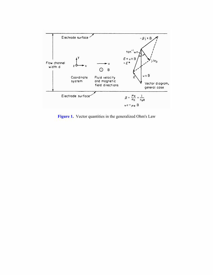
Figure 1. Vector quantities in the generalized Ohm's Law

z

xy

B

u

J

a

b

δ

++++++++++

– – – – – – –

Figure 2. Current paths in a conducting duct

1.00.80.60.40.20.00.0

0.2

0.4

0.6

0.8

1.0

1.2

1.4

1.6

Ha=0Ha=2Ha=5Ha=10Ha=50

z/a

Figure 3. Hartmann velocity profiles for Ha=0, 2, 5, 10, 50

(a)

(b)

Figure 4. Flow profiles in a square ( = 1) duct with Ha = 75, insulated side walls, andHartmann walls with F = 0.1: (a) velocity profile, (b) electric current paths

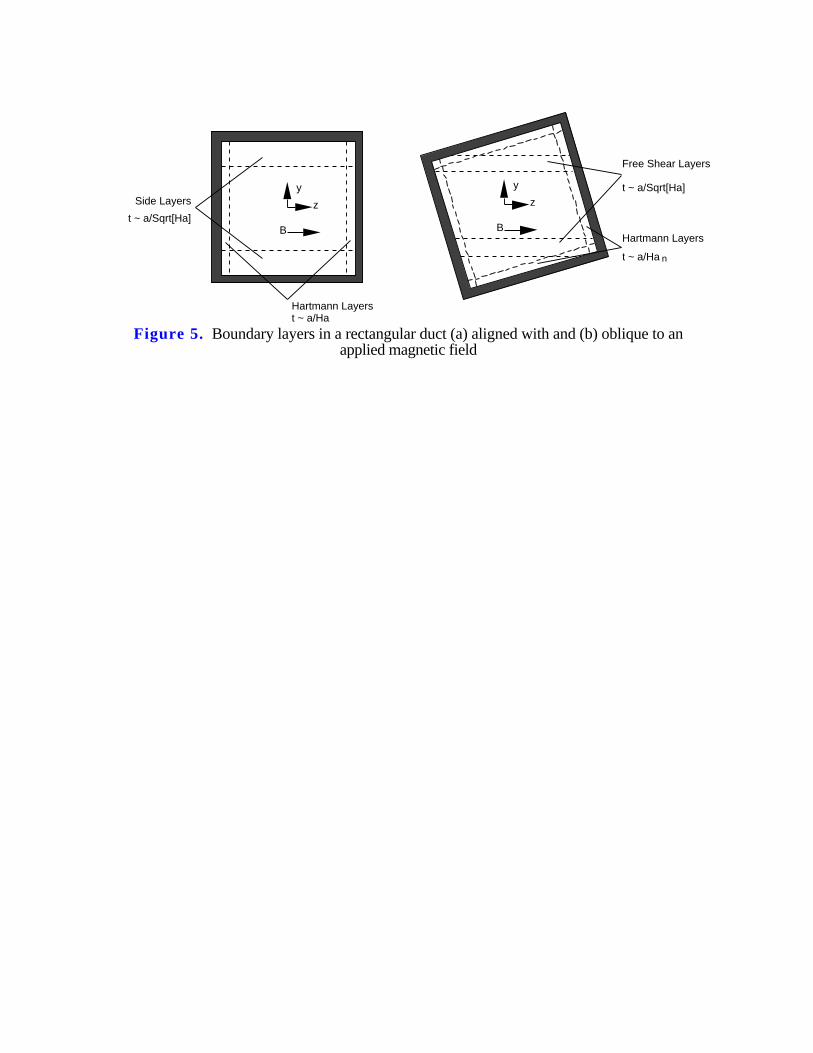
Side Layers

t ~ a/Sqrt[Ha]

Hartmann Layerst ~ a/Ha

y

z

B

y

z

B

Free Shear Layers

t ~ a/Sqrt[Ha]

Hartmann Layers

t ~ a/Ha n

Figure 5. Boundary layers in a rectangular duct (a) aligned with and (b) oblique to anapplied magnetic field

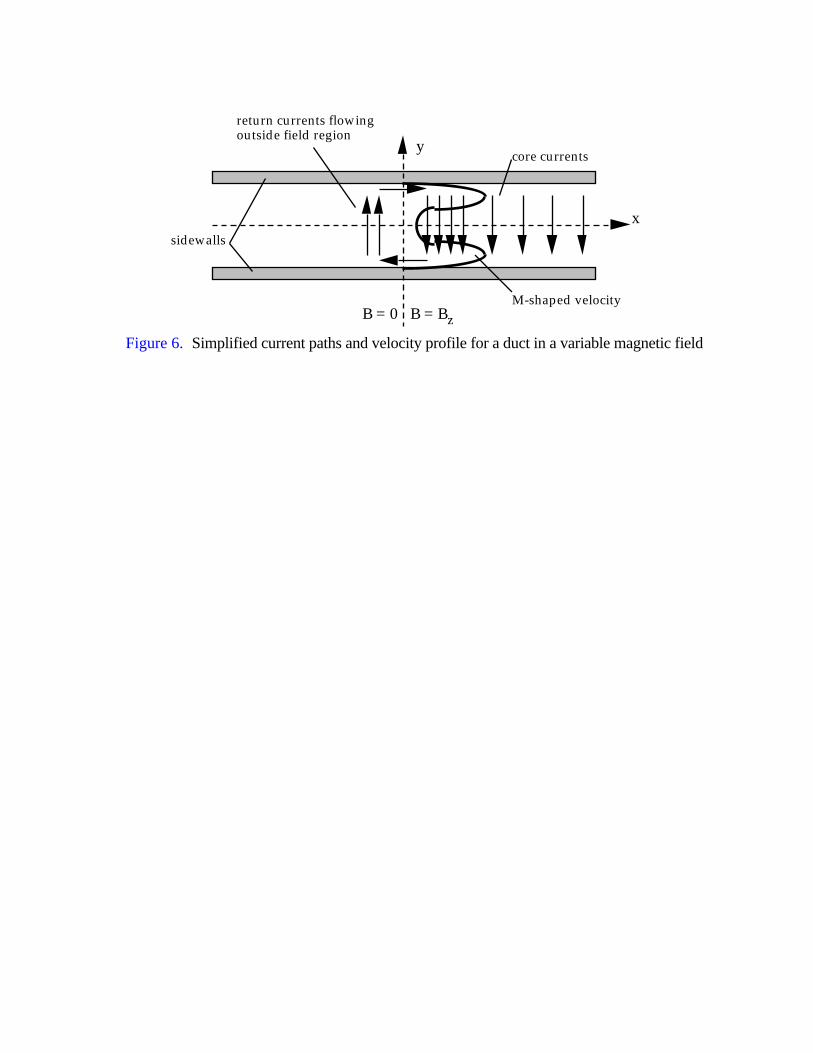
y

x

B = BzB = 0

core currents

return currents flowing outside field region

sidewalls

M-shaped velocity

Figure 6. Simplified current paths and velocity profile for a duct in a variable magnetic field

Applied Voltage

Magnet Yoke

Bus Bar

Magnet

Flow Channel

Figure 7. Generic DC conduction pump with rectangular channel

Voltage Signal Permanent Magnets

Iron Yoke

LM Flow

Figure 8. Generic DC EM flow meter

ILM ILoss

RLossRLMVa

Ia

Ei

+

+

–

–

Figure 9. Circuit network equivalent of a conduction pump

-10

0

10

20

30

40

0 2 4 6 8 10

Φ = 0Φ = 0.01Φ = 0.1

Dev

elop

ed P

ress

ure

(kP

a)

Flowrate (l/s)

Figure 10. Pressure head of a conduction pump for various wall conductance ratiosand the following parameters: a=5 cm, b=15 cm, L=30 cm,B=2 T (iron core electromagnet), Ia = 1500 amps, and σf = 106 Ω–1m–1

Peak magnetic field

Induced current loop

Windings and magnetic core

Channel wall

Direction of sliding fieldand pumping action

Figure 11. Operation of an induction pump

NSN –+–

Magnet Pole

Electrode

V and JxB

Figure 12. Turbulence reduction technique for seawater: alternating magnets andelectrodes [6,33]

Figure 13. Basic elements of a magnetohydrodynamic generator

Figure 14. Generator configurations: (a) segmented-electrode Faraday generator,(b) continuous-electrode Faraday generator, (c) Hall generator, and

(d) diagonally-connected generator.

Figure 15. Comparison of local electrical efficiencies of Faraday and Hall generators.

Figure 16. Dimensionless ratios vs. normalized length (x/Li) in an ideal,constant velocity channel.

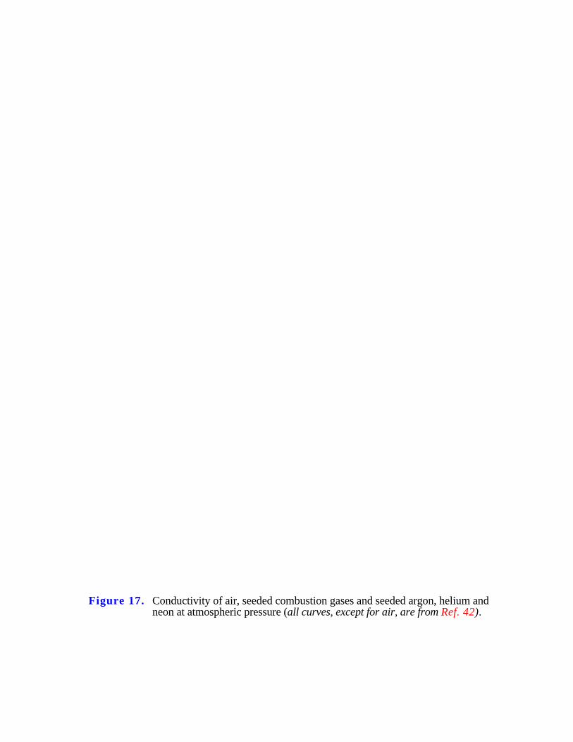
Figure 17. Conductivity of air, seeded combustion gases and seeded argon, helium andneon at atmospheric pressure (all curves, except for air, are from Ref. 42).

Figure 18. Conductivity vs. temperature and pressure for seeded coal products and airusing 1.5 wt.% K, obtained using dry K2CO3 (adaptedfrom Ref. 42).

Figure 19. Effect of magnetic field on two-phase flow regimes

1. recuperator (heated side)2. heat source3. turbine or LMMHD generator4. recuperator (cooled side)5. heat rejection6. compressors and intercoolers

T

s

1

2 3

4

56

T

s

1

2

3

4

56

Standard cycle LMMHD cycle

Figure 20. Standard Brayton cycle compared with MHD Brayton cycle

HeatSource

HeatSink

MHDGenerator

Evaporator Condensor

MHDPump

Figure 21. Homogeneous LMMHD cycle

HeatSource

HeatSink

MHDGenerator

Mixer Separator

MHDPump

Recuperator

2-phase compressor or Brayton cycle

thermodynamic fluid

electrodynamic fluid

Figure 22. Modified Ericsson cycle with LM heating