magnetometry measurements and first-order-reversal-curve

614.891.2243 | www.lakeshore.com

Magnetometry Measurements and First-Order-Reversal-Curve (FORC) AnalysisB. C. Dodrill

Lake Shore Cryotronics, Inc. | t. 614.891.2244 | [email protected] | www.lakeshore.com2

OVERVIEWMagnetometers are used to characterize magnetic material properties. Magnetometry techniques can be broadly classified into two categories: inductive and force-based. Common inductive methods include vibrating sample magnetometry (VSM), extraction magnetometry, AC susceptometry, and superconducting quantum interference device (SQUID) magnetometry. The two most commonly used inductive techniques are VSM and SQUID magnetometry. Alternating gradient magnetometry (AGM) is the most often used force-based technique. The measurement most commonly performed to characterize a material’s magnetic properties is that of a major hysteresis loop. The hysteresis or M(H) loop is typically used to determine a material’s saturation magnetization Ms (the magnetization at maximum applied field), remanence Mr (the magnetization at zero applied field after applying a saturating field), and coercivity Hc (the field required to demagnetize the material). More complex magnetization curves covering states with field and magnetization values located inside the major hysteresis loop, such as FORCs, can provide additional information that can be used to characterize magnetic interactions and coercivity distributions in magnetic materials1.

This e-book discusses some of the techniques currently used in the characterization of magnetic materials, and demonstrates the utility of the first-order-reversal-curve (FORC) measurement and analysis technique by presenting results for various magnetic materials.

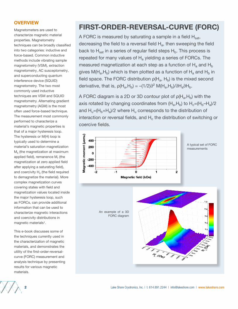
FIRST-ORDER-REVERSAL-CURVE (FORC)A FORC is measured by saturating a sample in a field Hsat, decreasing the field to a reversal field Ha, then sweeping the field back to Hsat in a series of regular field steps Hb. This process is repeated for many values of Ha yielding a series of FORCs. The measured magnetization at each step as a function of Ha and Hb gives M(Ha,Hb) which is then plotted as a function of Ha and Hb in field space. The FORC distribution ρ(Ha, Hb) is the mixed second derivative, that is, ρ(Ha,Hb) = –(1/2)∂² M(Ha,Hb)/∂Ha∂Hb.

A FORC diagram is a 2D or 3D contour plot of ρ(Ha,Hb) with the axis rotated by changing coordinates from (Ha,Hb) to Hc=(Hb–Ha)/2 and Hu=(Hb+Ha)/2 where Hu corresponds to the distribution of interaction or reversal fields, and Hc the distribution of switching or coercive fields.

A typical set of FORC measurements

An example of a 3D FORC diagram

Lake Shore Cryotronics, Inc. | t. 614.891.2244 | [email protected] | www.lakeshore.com 3

MAGNETIC MEASUREMENT TECHNIQUESVibrating sample magnetometry (VSM)

In vibrating sample magnetometry, originally developed by Simon Foner2 of MIT’s Lincoln Laboratory, a magnetic material is vibrated within a uniform magnetic field H, inducing an electric current in suitably placed sensing coils. The resulting voltage induced in the sensing coils is proportional to the magnetic moment of the sample. The magnetic field may be generated by an electromagnet or a superconducting magnet. VSM measurements can be performed from <2 K to 1273 K using integrated cryostats or furnaces.

Commercial VSM systems provide measurements to field strengths of ~3.4 T (34,000 Oe) using conventional electromagnets3,4, as well as systems employing superconducting magnets to produce fields to 16 T5,6. When used with electromagnets, very small step changes in field can be made (i.e., ~1 mOe) and the measurement is very fast. A typical hysteresis loop measurement can take as little as a few seconds to a few minutes.

Higher field strengths are possible with superconducting magnets; however, this limits the field setting resolution, and the measurement speed is inherently slower due to the speed at which the magnetic field can be varied using these magnets. Additionally, magnetometers employing superconducting magnets are more costly to operate since they require liquid helium. Cryogen-free systems employing closed cycle refrigeration systems are available but represent an expensive capital equipment investment. An advantage of superconducting magnet systems is they reach higher magnetic fields than air- or water-cooled electromagnets, which is necessary to saturate some magnetic materials, such as rare earth permanent magnets. The noise floor of commercially available VSMs is 10-7 to 10-8 emu.

Superconducting quantum interference device (SQUID) magnetometry

Quantum mechanical effects in conjunction with superconducting detection coil circuitry are used in SQUID-based magnetometers to measure the magnetic properties of materials. Theoretically, SQUIDs are capable of achieving sensitivities of 10-12 emu, but practically, they are limited to sensitivities of 10-8 emu because the SQUID also picks up environmental noise. As in a VSM, SQUIDs may be used to perform measurements from low to high temperatures (from <2 K to 1000 K). Superconducting magnets with field strengths up to 7 T are employed in SQUIDs5,6; therefore, the measurement is inherently slow due to the speed at which the magnetic field can be varied, as is the case for superconducting magnet-based VSM systems. A typical hysteresis M(H) loop measurement can take one hour or more.

Alternating gradient magnetometry (AGM)

Force methods involve determination of the apparent change in weight for a material when placed in an inhomogeneous magnetic field. The sample experiences a force f along the axis of the field gradient (dH/dz), which is given by f = m(dH/dz) where m is the magnetic moment. The equipment required for such force methods are either an electro- or superconducting magnet, and a balance for force measurements. A commercial variant of these methods is the alternating gradient magnetometer3. AGMs are capable of achieving sensitivities in the 10-8 to 10-9 emu range, and like the VSM, the AGM is a very fast measurement; a typical hysteresis loop takes seconds to minutes. Commercial AGM systems can be used for ambient temperature measurements to the moderate 2 – 3 T fields achievable with electromagnets.

Save time using faster acquisition methods

FORC measurements contain thousands if not tens of thousands of data points, and can be very time consuming (days to weeks) using superconducting magnet-based VSMs or SQUIDs. Electromagnet-based VSM and AGMs can acquire the data much more quickly (minutes to hours).

FORC STUDIESIn the pages that follow, we will also present FORC measurement results from various research papers in which either a VSM or AGM was used.

REFERENCES

1 C. R. Pike, A. P. Roberts, K. L. Verosub, “Characterizing Interactions in Fine Particle Systems Using First-Order-Reversal-Curves,” Journal of Applied Physics, 85, 6660, 1999.

2 S. Foner, Review of Scientific Instrumentation 30, 548 (1959), doi: 10.1063/1.1716679.

3 Lake Shore Cryotronics, USA; www.lakeshore.com

4 Microsense, USA; www.microsense.net

5 Quantum Design, USA; www.qdusa.com

6 Cryogenic Limited, UK; www.cryogenic.co.uk.


High-Temperature First-Order-Reversal-Curve (FORC) Study of Magnetic Nanoparticle Based Nanocomposite MaterialsTo be published in Proceedings of the 2016 XXV International Materials Research Congress (MRS Advances)

ABSTRACTFirst-order-reversal-curves (FORCs) are an elegant, nondestructive tool for characterizing the magnetic properties of materials comprising fine (micron- or nanoscale) magnetic particles. FORC measurements and analysis have long been the standard protocol used by geophysicists and earth and planetary scientists investigating the magnetic properties of rocks, soils, and sediments. FORC can distinguish between single-domain, multi-domain, and pseudo single-domain behavior, and it can distinguish between different magnetic mineral species1. More recently, FORC has been applied to a wider array of magnetic material systems because it yields information regarding magnetic interactions and coercivity distributions that cannot be obtained from major hysteresis loop measurements alone. In this paper, we will discuss this technique and present high-temperature FORC results for two magnetic nanoparticle materials: CoFe nanoparticles dispersed in a SiO₂ matrix, and FeCo-based nanocrystalline amorphous/nanocomposites.

INTRODUCTIONThe most common measurement that is performed to characterize a material’s magnetic properties is measurement of the major hysteresis loop M(H). The parameters that are most commonly extracted from the M(H) loop are: the saturation magnetization Ms, the remanence Mr, and the coercivity Hc.

First-order-reversal-curves (FORCs)2 can give information that is not possible to obtain from the hysteresis loop alone. These curves include the distribution of switching and interaction fields, and identification of multiple phases in composite or hybrid materials containing more than one phase3,4. A FORC is measured by saturating a sample in a field Hsat, decreasing the field to a reversal field Ha, then measuring moment versus field Hb as the field is swept back to Hsat. This process is repeated for many values of Ha, yielding a series of FORCs. The measured magnetization at each step as a function of Ha and Hb gives M(Ha, Hb), which is then plotted as a function of Ha and Hb in field space. The FORC distribution ρ(Ha, Hb) is the mixed second derivative, i.e., ρ(Ha, Hb) = -(1/2)∂2 M(Ha, Hb)/∂Ha∂Hb.

The FORC diagram is a 2D or 3D contour plot of ρ(Ha, Hb). It is common to change the coordinates from (Ha, Hb) to Hc = (Hb - Ha)/2 and Hu = (Hb + Ha)/2. Hu represents the distribution of interaction or reversal fields, and Hc represents the distribution of switching or coercive fields.

AUTHORS

B. Dodrill, Lake Shore Cryotronics, Inc., 575 McCorkle Blvd., Westerville, OH, USA

P. Ohodnicki, National Energy Technology Lab, 626 Cochrans Mill Road, Pittsburgh, PA, USA

M. McHenry and A. Leary, Carnegie Mellon University, Materials Science and Engineering, 5000 Forbes Ave., Pittsburgh, PA, USA

REFERENCES

1 A. R. Muxworthy, A. P. Roberts, “First-Order-Reversal-Curve (FORC) Diagrams,” Encyclopedia of Geomagnetism and Paleomagnetism. (Spring, 2007).

2 C. R. Pike, A. P. Roberts, K. L. Verosub, “Characterizing Interactions in Fine Particle Systems Using First Order Reversal Curves,” J. Appl. Phys. 85, 6660 (1999).

3 B. C. Dodrill, “First-Order-Reversal-Curve Analysis of Multi-phase Ferrite Magnets,” Magnetics Business and Technology. (Spring 2015).

4 C. Carvallo, A. R. Muxworthy, D. J. Dunlop, “First-Order-Reversal-Curve (FORC) Diagrams of Magnetic Mixtures: Micromagnetic Models and Measurements,” Physics of the Earth and Planetary Interiors. 154, 308 (2006).

5 P. R. Ohodnicki, Jr. V. Sokalski, J. Baltrus, J. B. Kortright, X. Zuo, S. Shen, V. Degeorge, M. E. McHenry, D. E. Laughlin, “Structure-Property Correlations in CoFe-SiO₂ Nanogranular Films Utilizing X-ray Photoelectron Spectroscopy and Small-Angle Scattering Techniques,” Journal of Electronic Materials 43 (1), 142 – 150 (2014).

6 S. Shen, P. R. Ohodnicki, S. J. Kernion, A. M. Leary, V. Keylin, J. F. Huth, M. E. McHenry, “Nanocomposite Alloy Design for High Frequency Power Conversion Applications,” https://www.researchgate.net/publication/236174216_Nanocomposite_Alloy_Design_for_High_Frequency_Power_Conversion_Applications.


EXPERIMENTTo demonstrate the utility of the FORC measurement and analysis protocol for characterizing high-temperature magnetic properties of materials, measurements were conducted for two different magnetic nanoparticle materials: CoFe nanoparticles dispersed in a SiO2 matrix5, and FeCo-based nanocrystalline amorphous/nanocomposites6,7. All magnetic measurements were performed using a Lake Shore Cryotronics MicroMag™ vibrating sample magnetometer (VSM) with a high-temperature furnace, enabling variable temperature measurements from room temperature to 800 °C. All measured magnetization data are presented in terms of the magnetic moment (emu) as a function of field (Oe) and temperature (°C). There are a number of open source FORC analysis software packages such as FORCinel8 and VARIFORC9. In this paper, FORCinel and custom analysis software were used to calculate the FORC distributions and plot the FORC diagrams.

DISCUSSIONCoFe Nanoparticles Dispersed in an SiO₂ Matrix

Figure 1 shows the room temperature hysteresis loops with SiO₂ volume fractions ranging from 40% to 80%, and show that the magnetic properties tend towards superparamagnetism with increasing SiO₂. Figure 2 shows the room temperature 2D FORC diagrams at SiO₂ volume fractions of 40%, 50%, and 60%. There is a single peak in each FORC distribution that is centered at Hc, and there is a distribution of both interaction (Hu, vertical axis) and switching fields (Hc, horizontal axis), the former due to interparticle interactions, and the latter due to different particles switching at different applied field strengths. Note that the peaks in the FORC distributions are shifted towards negative interaction fields (Hu, vertical axis) which is a feature that is typically associated with exchange interactions occurring between magnetic particles10.

-750

-500

-250

0

250

500

750

-400 -200 0 200 400

CoFe-SiOx Hysteresis Measurements

40%50%60%70%80%

M (e

mu/

cc)

Field (Oe)Figure 1. Room temperature hysteresis loops for CoFe nanoparticles dispersed in SiO2 with volume fractions ranging from 40% to 80% (data are volume normalized and presented in emu/cc).

7 J. Long, M. E. McHenry, D. E. Laughlin, C. Zheng, H. Kirmse, W. Neumann, “Analysis of Hysteretic Behavior in a FeCoB-based Nanocrystalline Alloy by a Preisach Distribution and Electron Holography,” J. Appl. Phys., 103, 07E710-12 (2008).

8 R. J. Harrison, J. M. Feinberg, “FORCinel: An Improved Algorithm for Calculating First-Order Reversal Curve Distributions Using Locally Weighted Regression Smoothing,” Geochemistry, Geophysics, Geosystems 9 11 (2008). FORCinel may be downloaded from: https://wserv4.esc.cam.ac.uk/nanopaleomag/?page_id=31.

9 R. Egli, “VARIFORC: An Optimized Protocol for Calculating Non-regular First-Order Reversal Curve (FORC) Diagrams,” Global and Planetary Change, 100, 203 (2013).

10 D. Roy, P. S. A. Kumar, “Exchange Spring Behaviour in SrFe12O19-CoFe₂O₄ Nanocomposites,” AIP Advances, 5 (2015).

11 B. F. Valcu, D. A. Gilbert, K. Liu, “Fingerprinting Inhomogeneities in Recording Media Using the First Order Reversal Curve Method,” IEEE Transactions on Magnetics, 47, 2988 (2011).

12 M. Winklhofer, R. K. Dumas, K. Liu, “Identifying Reversible and Irreversible Magnetization Changes in Prototype Patterned Media Using First- and Second-Order Reversal Curves,” J. Appl. Phys, 103, 07C518 (2008).

13 B. C. Dodrill, L. Spinu, “First-Order-Reversal-Curve Analysis of Nanoscale Magnetic Materials,” Technical Proceedings of the 2014 NSTI Nanotechnology Conference and Expo, CRC Press (2014).

14 B. C. Dodrill, “First-Order-Reversal-Curve Analysis of Nanocomposite Permanent Magnets,” Technical Proceedings of the 2015 TechConnect World Innovation Conference and Expo, CRC Press (2015).

15 B. C. Dodrill, “Magnetometry and First-Order-Reversal-Curve (FORC) Studies of Nanomagnetic Materials,” Dekker Encyclopedia of Nanoscience and Nanotechnology, Taylor & Francis (2016).


Figure 2. Room temperature 2D FORC diagrams for CoFe nanoparticles dispersed in SiO₂ volume fractions of 40% (left), 50% (middle), and 60% (right).

The hysteresis M(H) loops and FORCs were measured at temperatures of T = 25, 100, 200, 300, and 400 °C for the sample containing 40% volume fraction of CoFe nanoparticles dispersed in a 60% volume fraction of SiO₂. Transmission electron microscope (TEM) images show that the CoFe nanoparticles are approximately 10 nm in diameter and separated by an intergranular SiO₂ phase5. Figure 3 shows the hysteresis loops at each temperature and the measured FORCs at 25 °C. Figure 4 shows the 2D FORC diagrams at temperatures ranging from 25 to 400 °C. There is a single peak in the FORC distribution at each temperature that is centered at Hc and that shifts towards lower switching fields as temperature increases, coincident with the decrease in Hc with increasing temperature. In a FORC diagram, entirely closed contours are typically considered to be a fingerprint of single-domain (SD) particles, whereas entirely open contours that diverge towards the Hu axis are a fingerprint of multi-domain (MD) behavior1. The results shown in figure 4 demonstrate closed contours at lower temperatures and open contours at increasing temperatures, suggesting a transition from SD to MD behavior based upon the conventional interpretation of FORC diagrams. Further studies are required to better understand if this traditional interpretation is valid for such densely packed nanoparticle aggregates. At all temperatures there is a distribution of both interaction (Hu, vertical axis) and switching fields (Hc, horizontal axis), the former owing to interparticle interactions, and the latter due to different particles switching at different applied field strengths.

-0.0003-0.0002-0.0002-0.0001-0.00010.00000.00010.00010.00020.00020.0003

-500 -250 0 250 500

Mom

ent(

emu)

Field (Oe)

-0.00025-0.00020-0.00015-0.00010-0.000050.000000.000050.000100.000150.000200.00025

-750 -500 -250 0 250 500 750

Mom

ent(

emu)

Field (Oe)

25 °C100 °C200 °C300 °C400 °C

Figure 3. Hysteresis loops at T = 25, 100, 200, 300, and 400 °C (left) and measured FORCs at 25 °C (right) for CoFe nanoparticles (40%) dispersed in SiO₂ (60%).


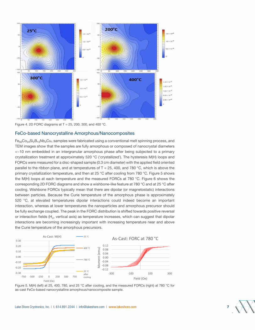
Figure 4. 2D FORC diagrams at T = 25, 200, 300, and 400 °C.

FeCo-based Nanocrystalline Amorphous/Nanocomposites

Fe56Co24Si2B13Nb4Cu1 samples were fabricated using a conventional melt spinning process, and TEM images show that the samples are fully amorphous or composed of nanocrystal diameters <~10 nm embedded in an intergranular amorphous phase after being subjected to a primary crystallization treatment at approximately 520 °C (‘crystallized’). The hysteresis M(H) loops and FORCs were measured for a disc-shaped sample (0.3 cm diameter) with the applied field oriented parallel to the ribbon plane, and at temperatures of T = 25, 400, and 780 °C, which is above the primary crystallization temperature, and then at 25 °C after cooling from 780 °C. Figure 5 shows the M(H) loops at each temperature and the measured FORCs at 780 °C. Figure 6 shows the corresponding 2D FORC diagrams and show a wishbone-like feature at 780 °C and at 25 °C after cooling. Wishbone FORCs typically mean that there are dipolar (or magnetostatic) interactions between particles. Because the Curie temperature of the amorphous phase is approximately 520 °C, at elevated temperatures dipolar interactions could indeed become an important interaction, whereas at lower temperatures the nanoparticles and amorphous precursor should be fully exchange coupled. The peak in the FORC distribution is shifted towards positive reversal or interaction fields (Hu, vertical axis) as temperature increases, which can suggest that dipolar interactions are becoming increasingly important with increasing temperature near and above the Curie temperature of the amorphous precursors.

-0.30

-0.20

-0.10

0.00

0.10

0.20

0.30

-750 -500 -250 0 250 500 750

Mom

ent (

emu)

Field (Oe)

As-Cast: M(H) 25 °C

400 °C

780 °C

25 °Ca�ercooling

-0.12-0.08-0.040.000.040.080.12

-300 -100 100 300

Mom

ent (

emu)

Field (Oe)

As-Cast: FORC at 780 °C

Figure 5. M(H) (left) at 25, 400, 780, and 25 °C after cooling, and the measured FORCs (right) at 780 °C for as-cast FeCo-based nanocrystalline amorphous/nanocomposite sample.


Figure 6. 2D FORC diagrams at 25 (upper left), 400 (upper right), 780 (lower left), and 25 °C after cooling (lower right) for a as-cast FeCo-based nanocrystalline amorphous/nanocomposites.

CONCLUSIONSFORC analysis is indispensable for characterizing interactions and coercivity distributions in a wide array of magnetic materials, including; natural magnets, magnetic recording media11,12, nanowire arrays13, permanent magnets14, and exchanged coupled magnetic multilayers15. In this paper, we have shown the evolution at high temperatures of the distribution of switching and interaction fields as determined from FORC analysis for CoFe nanoparticles and FeCo-based nanocrystalline magnetic materials


High-Temperature First-Order-Reversal-Curve (FORC) Study of Single- and Multi-Phase Permanent MagnetsMaterials Research Bulletin, Vol. 40, Issue 11, November 2015

ABSTRACTFirst-order-reversal-curves (FORCs) are a nondestructive tool for characterizing the magnetic properties of materials comprised of fine (micron- or nanoscale) magnetic particles. FORC measurements and analysis have long been the standard protocol used by geophysicists and earth and planetary scientists investigating the magnetic properties of rocks, soils, and sediments. A FORC can distinguish between single-domain, multi-domain, and pseudo single-domain behavior, and it can distinguish between different magnetic mineral species1. More recently, FORC has been applied to a wider array of magnetic material systems, because it yields information regarding magnetic interactions and coercivity distributions that cannot be obtained from measurements of a material’s major hysteresis loop alone. In this article, we discuss the FORC measurement and analysis technique and present high-temperature FORC results for multi-phase permanent magnets.

MAGNETIZATION MEASUREMENTS AND FIRST-ORDER-REVERSAL-CURVESThe most common measurement that is performed to characterize a material’s magnetic properties is measurement of the major hysteresis loop M(H) using either a vibrating sample magnetometer or superconducting quantum interference device magnetometer. The parameters that are most commonly extracted from the M(H) loop are the saturation magnetization Ms, the remanence Mr, and the coercivity Hc. In a hysteresis loop measurement, the measured coercivity Hc is the weighted coercivity of the entire ensemble of magnetic particles that constitute a magnetic material, thus if the material contains more than one magnetic phase, it is hard to discern between these phases.

FORCs2 can give information that is not possible to obtain from the hysteresis loop alone. This includes the distribution of switching and interaction fields, and identification of multiple phases in composite or hybrid materials containing more than one phase3,4. A FORC is measured by saturating a sample in a field Hsat, decreasing the field to a reversal field Ha, then measuring moment versus field Hb as the field is swept back to Hsat. This process is repeated for many values of Ha, yielding a series of FORCs. The measured magnetization at each step as a function of Ha and Hb gives M(Ha, Hb), which is then plotted as a function of Ha and Hb in field space. The FORC distribution ρ(Ha, Hb) is the mixed second derivative, ρ(Ha, Hb) = –(1/2)∂² M(Ha, Hb)/∂Ha∂Hb.

The FORC diagram is a 2D or 3D contour plot of ρ(Ha, Hb). It is common to change the coordinates from (Ha, Hb) to Hc = (Hb – Ha)/2 and Hu = (Hb + Ha)/2, where Hu represents the distribution of interaction or reversal fields, and Hc represents the distribution of switching or coercive fields.

AUTHORS

B. C. Dodrill, J. Lindemuth, C. Radu, Lake Shore Cryotronics

H. Reichard, Princeton Measurement Corp. [email protected]

REFERENCES

1 A. R. Muxworthy, A. P. Roberts, “Encyclopedia of Geomagnetism and Paleomagnetism,” D. Gubbins, E. Herrero-Ververa, Eds. (Springer, The Netherlands, 2007), pp. 266 – 272.

2 C. R. Pike, A. P. Roberts , K. L. Verosub, Journal of Applied Physics 85, 6660 (1999).

3 B. C. Dodrill, Magnetics Business and Technology 8 (Spring 2015).

4 C. Carvallo , A. R. Muxworthy , D. J. Dunlop, Physics of the Earth and Planetary Interiors 154, 308 (2006).

5 R. J. Harrison , J. M. Feinberg, Geochemistry Geophysics Geosystems 9, 11 (2008).

6 R. Egli, Global and Planetary Change 203, 110 (2013).


HIGH-TEMPERATURE FORC RESULTS FOR MULTI-PHASE PERMANENT MAGNETSTo demonstrate the utility of the FORC measurement and analysis protocol for magnetic property measurements, the characterization of high-temperature magnetic properties of materials is presented. Measurements were conducted for a synthetically produced three-phase magnet by mixing together, in approximate equal mass proportions, three different single-phase magnets: Sr-ferrite powder (Hoosier Magnetics), BaSr ceramic (Magnet Sales & Manufacturing – Integrated Magnetics), and sintered NdFeB (Magnequench). All magnetic measurements were performed using a Lake Shore Cryotronics MicroMag™ vibrating sample magnetometer with a high-temperature furnace, which allows for variable temperature measurements from room temperature to 800 °C. All measured magnetization data are presented in terms of the magnetic moment (emu) as a function of field (Oe) and temperature (°C). There are a number of open source FORC analysis software packages such as FORCinel5 and VARIFORC6, although in this paper, custom analysis software was used to calculate the FORC distributions and plot the FORC diagrams.

Figure 1 shows the hysteresis M(H) loops at temperatures of T = 25 °C, 200 °C, 300 °C, 375 °C, and 450 °C (a) and the temperature dependence of the coercivity (b) for the individual samples and three-phase mixture. The M(H) loops at 25 °C and 450 °C show evidence of a two-step and thus two-phase behavior, while the loops at intermediate temperatures essentially exhibit single-phase behavior. There is no suggestion of three-phase behavior in any of the measured M(H) loops.

Figure 1. (a) M(H) at T = 25 °C, 200 °C, 300 °C, 375 °C, and 450 °C for a three-phase mixture of Sr-ferrite powder, BaSr ceramic, and sintered NdFeB, and (b) Hc versus T plots for the individual samples and the three-phase mixture.

Figure 2 shows the measured FORCs at temperatures of T = 25 °C, 200 °C, 300 °C, 375 °C, and 450 °C and at 25 °C after cooling from 450 °C.

Figure 3 shows the 2D FORC diagrams at each temperature. At 25 °C, there are three peaks in the FORC distribution corresponding to each phase. At 200 °C, the BaSr and NdFeB peaks are not separable because their coercivities are very similar; although at temperatures above 200 °C, each phase is again distinguishable, with the NdFeB peak shifting toward lower switching fields coincident with the decrease in its coercivity with increasing temperature. The Sr-ferrite and BaSr peaks initially shift toward higher switching fields and then move toward lower switching fields with increasing temperature. This coincides with the temperature dependence of their coercivity, as determined from their M(H) loop measurements.


Figure 2. Measured FORCs at T = (a) 25 °C, (b) 200 °C, (c) 300 °C, (d) 375 °C, (e) 450 °C, and (f) 25 °C after cooling from 450 °C for a three-phase mixture of Sr-ferrite powder, BaSr ceramic, and sintered NdFeB.

Figure 3. 2D FORC diagrams at T = (a) 25 °C, (b) 200 °C, (c) 300 °C, (d) 375 °C, (e) 450 °C, and (f) 25 °C after cooling from 450 °C for a three-phase mixture of Sr-ferrite powder, BaSr ceramic, and sintered NdFeB.

From FORC measurements of the single-phase samples, it is known that the ridge feature (see Figure 3) is related to the NdFeB. The ridge continuously shifts toward lower switching fields and less negative interaction fields with increasing temperature, and is believed to be due to temperature-induced magnetostatic interactions. Also there is a fourth peak of unknown origin present in the distribution at 300 °C located between the Sr-ferrite and NdFeB peaks. At 450 °C, there is no feature associated with the NdFeB because its coercivity is small, and the ridge has entirely disappeared. Finally, the last FORC diagram shows results at 25 °C after cooling from 450 °C and depicts the reemergence of the NdFeB peak and ridge. In comparing the FORC diagrams at 25 °C before warming and after cooling, there are obvious differences owing to irreversible changes in the material resulting from thermal cycling.


CONCLUSIONSFORC analysis has been shown to be very useful for characterizing interactions and coercivity distributions in an array of magnetic materials, including magnetic nanowire arrays, permanent magnets, magnetic recording media, exchange-biased magnetic multilayer thin films, and natural magnets. We have shown the evolution at high temperatures of the distribution of switching and interaction fields as determined from FORC analysis for a three-phase mixture of three single-phase magnets. The results demonstrate the utility of FORC analysis for differentiating phases in multi-phase magnetic materials. The results shown in the figures are based on unpublished data.


First-Order-Reversal-Curve (FORC) Analysis of Multi-Phase Ferrite MagnetsMagnetics Business & Technology, March 2015

ABSTRACTMagnetically hard ferrite powders are widely used, due to their low-cost production and good performance in many electronic devices such as electrical motors, speakers and recording media. Usually ferrites are single-phase magnets but when the stoichiometry is not precise or the fabrication process is not adequate, the ferritic phase may be accompanied by other phases that promote magnetic interactions, which results in a decrease of the magnetic performance of the magnet. Additionally, there is currently strong interest in exchange spring magnets, which are comprised of a hard high coercivity phase exchange coupled to a soft high saturation magnetization phase, as this leads to a magnet with increased energy density. This results in reduced costs because less hard phase material is required. Other examples of multiphase magnets include nanostructures, such as soft shell/hard core nanowires, hybrid magnets, etc. The magnetic characterization of such materials is usually made by measuring a hysteresis loop. However, it is very difficult to unravel the complex magnetic signatures of multi-phase magnets, or to obtain information of interactions or coercivity distributions from the hysteresis loop alone. First-order-reversal-curves (FORCs) provide a means for determining the distribution of switching and interaction fields between magnetic particles, and for distinguishing between magnetic phases in composite materials that contain more than one magnetic phase. In this article, we will discuss the FORC measurement and analysis technique, and present results for various ferrite multi-phase composites.

MAGNETIZATION MEASUREMENTS AND FIRST-ORDER-REVERSAL-CURVESThe most common measurement that is performed to characterize a materials magnetic properties is measurement of the major hysteresis or M(H) loop. The parameters that are usually extracted from the M(H) loop are illustrated in Figure 1 and include: the saturation magnetization Msat (the magnetization at maximum applied field), the remanence Mrem (the magnetization at zero applied field after applying a saturating field), and the coercivity Hc (the field required to demagnetize the material). For permanent magnet materials, the maximum energy product BHmax, which is determined from the second quadrant demagnetization curve, is also commonly of interest. Note that the measured coercivity Hc is the average coercivity (or average distribution of switching fields) of the entire ensemble of magnetic particles that constitute a magnetic material.

AUTHOR

B. Dodrill, Lake Shore Cryotronics

REFERENCES


2 B. C. Dodrill, L. Spinu, “First-Order-Reversal-Curve-Analysis of Nanoscale Magnetic Materials,” Technical Proceedings of the 2014 NSTI Nanotechnology Conference, CRC Press, June 2014.

3 R. J. Harrison and J. M. Feinberg, “FORCinel: An Improved Algorithm for Calculating First-Order-Reversal-Curve Distributions Using Locally Weighted Regression Smoothing,” Geochemisty, Geophysics, Geosystems, 9, 11, 2008. FORCinel may be downloaded from: https://wserv4.esc.cam.ac.uk/nanopaleomag/?page_id=31.

4 B. C. Dodrill, “FORC Analysis of Permanent Magnet Materials,” Lake Shore Application Note (and references contained therein).

5 B. C. Dodrill, L. Spinu, “FORC Analysis of Exchange Bias Magnetic Multilayer Films,” Lake Shore Application Note (and references contained therein).

6 A. R. Muxworthy, A. P. Roberts, “First-Order-Reversal-Curve (FORC) Diagrams,” Encyclopedia of Geomagnetism and Paleomagnetism, Springer, 2007.


Figure 1. Hysteresis M(H) loop for a NdFeB sample.

More complex magnetization curves covering states with field and magnetization values located inside the major hysteresis loop, such as first-order-reversal-curves (FORCs)1, can give information that is not possible to obtain from the hysteresis loop alone. These curves include the distribution of switching and interaction fields, and differentiation of multiple phases in composite or hybrid materials containing more than one phase. A FORC is measured by saturating a sample in a field Hsat, decreasing the field to a reversal field Ha, then sweeping the field back to Hsat in a series of regular field steps Hb. This process is repeated for many values of Ha, yielding a series of FORCs. This is illustrated in Figure 2. The measured magnetization at each step as a function of Ha and Hb gives M(Ha, Hb), which is then plotted as a function of Ha and Hb in field space. The FORC distribution ρ(Ha, Hb) is the mixed second derivative, i.e., ρ(Ha, Hb) = -(1/2)∂2 M(Ha, Hb)/∂Ha∂Hb.

Figure 2. Measured first-order-reversal curves for a ferrite permanent magnet.

The FORC diagram is a 2D or 3D contour plot of ρ(Ha, Hb) with the axis rotated by changing coordinates from (Ha, Hb) to Hc = (Hb - Ha)/2 and Hu = (Hb + Ha)/2, as illustrated in Figure 3, where Hu represents the distribution of interaction fields, and Hc represents the distribution of switching fields.


Figure 3. A 2D FORC diagram for a periodic array of Ni nanowires showing the distribution of switching (Hc) and interaction (Hu) fields2.

FORC RESULTS FOR MULTI-PHASE FERRITE MAGNETSTo demonstrate the utility of FORC analysis for differentiating multiple phase materials, multi-phase composites were synthetically produced by mixing together single-phase magnets including: Sr-ferrite powder, BaFe₂O₄ ceramic, and BaFe₂O₄ and γ-Fe₂O₃ magnetic recording tapes. All magnetic measurements were performed at ambient temperature using a Lake Shore Cryotronics MicroMag™ vibrating sample magnetometer (VSM). There are a number of open source FORC analysis software packages such as FORCinel3, although in this article custom analysis software was used to calculate the FORC distributions.

Figure 4 and Figure 5 show the measured hysteresis M(H) loop and FORCs for a sample consisting of a mixture of Sr-ferrite powder and BaFe₂O₄ ceramic. The coercivities for each sample as determined from their individual M(H) loops were 1 kOe and 3 kOe, respectively. The coercivity for the mixed sample is 2.3 kOe and there is no clear evidence of multi-phase behavior from the M(H) loop results shown in Figure 4.

Figure 4. Hysteresis M(H) loop for a mixture of Sr-ferrite powder and BaFe₂O₄ ceramic.


Figure 5. FORCs for a mixture of Sr-ferrite powder and BaFe₂O₄ ceramic.

Figure 6 shows the 2D FORC diagram for the mixture of Sr-ferrite powder and BaFe₂O₄ ceramic. There are two peaks in the distribution centered at 1 kOe and 3 kOe corresponding to the Sr-ferrite powder and BaFe₂O₄ ceramic, respectively.

Figure 6. 2D FORC diagram showing the distribution of switching (Hc) and interaction (Hu) fields for a mixture of Sr-ferrite powder and BaFe₂O₄ ceramic, showing the phases of each individual material clearly differentiated.


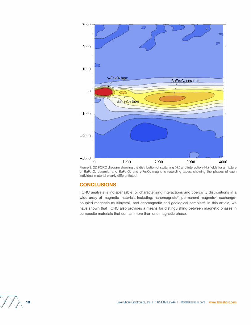
Figure 7 shows the individual and combined M(H) loops for a synthetically produced 3-phase sample, consisting of a BaFe₂O₄ ceramic, and BaFe₂O₄ (MT1) and γ-Fe₂O₃ (MT2) magnetic recording tapes with individual coercivities (as determined from the individual M(H) loops) of 2 kOe, 789 Oe, and 233 Oe, respectively. Note that the M(H) loop for the mixture of all three samples is very similar to the hysteresis loop for the BaFe₂O₄ ceramic sample alone, and is devoid of any indication of multi-phase behavior.

Figure 7. Measured M(H) loops for a BaFe₂O₄ ceramic, BaFe₂O₄, and γ-Fe₂O₃ magnetic recording tapes, and the mixture of all three samples (note: the M(H) loops for the ceramic and combined samples have been re-scaled to present all loops on the same scale).

Figure 8 and Figure 9 show the measured FORCs and 2D FORC diagram, respectively, for the mixture of all three samples. There are three peaks in the distribution centered at the coercivities corresponding to each individual sample.

Figure 8. Measured FORCs for a mixture of BaFe₂O₄ ceramic, and BaFe₂O₄ and γ-Fe₂O₃ magnetic recording tapes.


Figure 9. 2D FORC diagram showing the distribution of switching (Hc) and interaction (Hu) fields for a mixture of BaFe₂O₄ ceramic, and BaFe₂O₄ and γ-Fe₂O₃ magnetic recording tapes, showing the phases of each individual material clearly differentiated.

CONCLUSIONSFORC analysis is indispensable for characterizing interactions and coercivity distributions in a wide array of magnetic materials including: nanomagnets2, permanent magnets4, exchange-coupled magnetic multilayers5, and geomagnetic and geological samples6. In this article, we have shown that FORC also provides a means for distinguishing between magnetic phases in composite materials that contain more than one magnetic phase.


First-Order-Reversal-Curve (FORC) Study of Nanocomposite Permanent MagnetsTechnical Proceedings of the 2015 TechConnect World Innovation Conference and Expo, CRC Press, June 2015

ABSTRACTThe magnetic properties of permanent magnet materials are usually characterized by measuring a hysteresis loop using a vibrating sample magnetometer (VSM). Nanocomposite permanent magnets consist of a dispersion of nanoscale magnetic particles that can contain more than one magnetic phase, and interactions between particles can impact the magnetic performance of the magnet. It is not possible to unravel the complex magnetic signatures of multiphase materials and to obtain information of interactions or coercivity distributions from the hysteresis loop alone. First-order-reversal-curves (FORCs) provide a means for determining the distribution of interaction fields between magnetic particles, and for distinguishing between magnetic phases in composite materials that contain more than one magnetic phase. In this paper, we will discuss the FORC measurement and analysis technique, and present results for various multiphase nanocomposite magnets.

INTRODUCTIONRare-earth and ferrite permanent magnet materials are indispensable elements in many electronic devices such as electrical motors, hybrid vehicles, portable communications devices, speakers, sensors, etc. The magnets have major influence on the size, efficiency, stability, and cost of these devices and systems.

Owing to the decreased availability and increasing cost of rare-earth elements, significant research is underway to develop strong permanent magnet materials that do not rely as heavily on rare-earth constituents. These can include nanocomposite exchange spring magnets comprised of a hard high coercivity phase, exchange coupled to a soft high saturation magnetization phase, which increases the energy density and decreases the cost of the magnet because less hard phase material is needed; multi-phase composite nanostructures such as soft shell/hard core magnetic nanowires; and hybrid magnets, etc.

Additionally, magnetically hard ferrite nano- or micron-scale powders are widely used owing to their low-cost production and good performance in many electronic devices and magnetic storage media. When the stoichiometry is not precise or the fabrication process is not adequate, however, the ferritic phase is accompanied by other phases that promote magnetic interactions that results in a decrease of the magnetic performance of the magnet.

The magnetic characterization of such materials is usually made by measuring a hysteresis loop using a vibrating sample magnetometer (VSM). It is very difficult, however, to unravel the complex magnetic signatures of multiphase materials and obtain information of interactions or coercivity distributions from the hysteresis loop alone. First-order-reversal-curves (FORCs) provide a means for determining the distribution of interaction fields between magnetic particles, and for distinguishing between magnetic phases in composite materials that contain more than one magnetic phase. In this paper we will discuss the FORC measurement and analysis technique, and present results for various multiphase nanocomposite magnets.

AUTHOR

B. Dodrill, Lake Shore Cryotronics

REFERENCES


2 B. C. Dodrill, L. Spinu, “First-Order-Reversal-Curve-Analysis of Nanoscale Magnetic Materials,” Technical Proceedings of the 2014 NSTI Nanotechnology Conference, CRC Press, June 2014.

3 R. J. Harrison and J. M. Feinberg, “FORCinel: An Improved Algorithm for Calculating First-Order-Reversal-Curve Distributions Using Locally Weighted Regression Smoothing,” Geochemisty, Geophysics, Geosystems, 9, 11, 2008. FORCinel may be downloaded from: https://wserv4.esc.cam.ac.uk/nanopaleomag/?page_id=31.

4 B. C. Dodrill, “FORC Analysis of Permanent Magnet Materials,” Lake Shore Application Note (and references contained therein).

5 B. C. Dodrill, L. Spinu, “FORC Analysis of Exchange Bias Magnetic Multilayer Films,” Lake Shore Application Note (and references contained therein).

6 A. R. Muxworthy, A. P. Roberts, “First-Order-Reversal-Curve (FORC) Diagrams,” Encyclopedia of Geomagnetism and Paleomagnetism, Springer, 2007.


MAGNETIZATION MEASUREMENTS AND FIRST-ORDER-REVERSAL-CURVES (FORCS)The most common measurement that is performed to characterize a materials’ magnetic properties is measurement of the major hysteresis or M(H) loop. The parameters that are usually extracted from the M(H) loop are illustrated in Figure 1 and include: the saturation magnetization Msat (the magnetization at maximum applied field), the remanence Mrem (the magnetization at zero applied field after applying a saturating field), and the coercivity Hc (the field required to demagnetize the material). For permanent magnet materials, the maximum energy product BHmax, which is determined from the second quadrant demagnetization curve, is also commonly of interest. Note that the measured coercivity Hc is the average coercivity (or average distribution of switching fields) of the entire ensemble of magnetic particles that constitute a magnetic material.

Figure 1. Hysteresis M(H) loop for NdFeB nanoparticles.

More complex magnetization curves covering states with field and magnetization values located inside the major hysteresis loop, such as first-order-reversal-curves (FORCs)1, can give information that is not possible to obtain from the hysteresis loop alone. These curves include the distribution of switching and interaction fields and differentiation of multiple phases in composite or hybrid materials containing more than one phase. A FORC is measured by saturating a sample in a field Hsat, decreasing the field to a reversal field Ha, then sweeping the field back to Hsat in a series of regular field steps Hb. This process is repeated for many values of Ha, yielding a series of FORCs. This is illustrated in Figure 2. The measured magnetization at each step as a function of Ha and Hb gives M(Ha, Hb), which is then plotted as a function of Ha and Hb in field space. The FORC distribution ρ(Ha, Hb) is the mixed second derivative, i.e., ρ(Ha, Hb) = -(1/2)∂2 M(Ha, Hb)/ ∂Ha∂Hb.


Figure 2. Measured first-order-reversal-curves for a ferrite permanent magnet.

The FORC diagram is a 2D or 3D contour plot of ρ(Ha, Hb) with the axis rotated by changing coordinates from (Ha, Hb) to Hc = (Hb - Ha)/2 and Hu = (Hb + Ha)/2, as illustrated in Figure 3, where Hu represents the distribution of interaction fields, and Hc represents the distribution of switching fields.

Figure 3. A 2D FORC diagram for a periodic array of Ni nanowires showing the distribution of switching (Hc) and interaction (Hu) fields2.


FORC RESULTS FOR MULTI-PHASE NANOCOMPOSITE FERRITE MAGNETSTo demonstrate the utility of FORC analysis for differentiating multiple phase materials, multi-phase composites were synthetically produced by mixing together single-phase magnets including: Sr-ferrite and Ba-ferrite nanoparticles, and yttrium-iron-garnet (YIG) and Co-doped YIG nanoparticles. All magnetic measurements were performed at ambient temperature using a Lake Shore Cryotronics MicroMag™ vibrating sample magnetometer (VSM). There are a number of open source FORC analysis software packages such as FORCinel3, although in this paper custom analysis software was used to calculate the FORC distributions.

Figure 4 and Figure 5 show the measured hysteresis M(H) loop and FORCs for a sample consisting of a mixture of Sr-ferrite and Ba-ferrite nanoparticles. The coercivities for each sample as determined from their individual M(H) loops were 1 kOe and 3 kOe, respectively. The coercivity for the mixed sample is 2.3 kOe and there is no clear evidence of multi-phase behavior from the M(H) loop results shown in Figure 4.

-0.6

-0.4

-0.2

0.0

0.2

0.4

0.6

-10,000 -8,000 -6,000 -4,000 -2,000 0 2,000 4,000 6,000 8,000 10,000

Mom

ent (

emu)

Field (Oe)

Ceramic Ferrite + HM206

Figure 4. Hysteresis M(H) loop for a mixture of Sr-ferrite and Ba-ferrite nanoparticles.

Figure 5. FORCs for a mixture of Sr-ferrite and Ba-ferrite nanoparticles.


Figure 6 shows the 2D FORC diagram for the mixture of Sr-ferrite and Ba-ferrite nanoparticles. There are two peaks in the distribution centered at 1 kOe and 3 kOe, corresponding to the Sr-ferrite and Ba-ferrite, respectively.

Figure 6. 2D FORC diagram showing the distribution of switching (Hc) and interaction (Hu) fields for a mixture of Sr-ferrite and Ba-ferrite nanoparticles, showing the phases of each individual material clearly differentiated.

Figure 7 shows the M(H) loop for a mixture consisting of a yttrium-iron-garnet (YIG) and Co-doped YIG nanoparticles with individual coercivities (as determined from the individual M(H) loops) of 71 Oe and 950 Oe, respectively. The M(H) loop is devoid of any indication of multi-phase behavior.

-0.08

-0.06

-0.04

-0.02

0.00

0.02

0.04

0.06

0.08

-15,000 -10,000 -5,000 0 5,000 10,000 15,000

Mom

ent (

emu)

Field (Oe)

Figure 7. Measured M(H) loops for a mixture of YIG and Co-doped YIG nanoparticles.


Figure 8 and Figure 9 show the measured FORCs and 2D FORC diagram, respectively, for the mixture of YIG and Co-doped YIG nanoparticles. There are two peaks in the distribution centered at 71 Oe and 950 Oe, corresponding to the YIG and Co-doped YIG nanoparticles, respectively.

-0.05

-0.04

-0.03

-0.02

-0.01

0.00

0.01

0.02

0.03

0.04

0.05

-4,000 -3,000 -2,000 -1,000 0 1,000 2,000 3,000 4,000

Mom

ent (

emu)

Field (Oe)

Figure 8. Measured FORCs for a mixture of YIG and Co-doped YIG nanoparticles.

Figure 9. 2D FORC diagram showing the distribution of switching (Hc) and interaction (Hu) fields for a mixture of YIG and Co-doped YIG nanoparticles.

CONCLUSIONSFORC analysis is indispensable for characterizing interactions and coercivity distributions in a wide array of magnetic materials including: nanomagnets2, permanent magnets4, exchange-coupled magnetic multilayers5, and geomagnetic and geological samples6. In this paper, we have shown that FORC also provides a means for distinguishing between magnetic phases in composite materials that contain more than one magnetic phase.


First-Order-Reversal-Curve (FORC) Analysis of Nanoscale Magnetic MaterialsTechnical Proceedings of the 2014 NSTI Nanotechnology Conference, June 2014

ABSTRACTMagnetic nanowires, nanodots, and nanoparticles are an important class of nanostructured magnetic materials. At least one of the dimensions of these structures is in the nanometer (nm) range and thus, new phenomena arise in these materials due to size confinement. These structures are ideal candidates for important technological applications in spintronics, high density recording media, microwave electronics, permanent magnets, and for medical diagnostics and targeted drug delivery applications. In addition to these technological applications, these materials represent an experimental playground for fundamental studies of magnetic interactions and magnetization mechanisms at the nanoscale level. When investigating the magnetic interactions in these materials, one of the most interesting configurations is a periodic array of magnetic nanowires, because both the size of the wires and their arrangement with respect to one another can be controlled. Inter-wire coupling is one of the most important effects in nanowire arrays because it significantly affects magnetization switching, and microwave and magneto-transport properties. The magnetic characterization of materials is usually made by measuring a hysteresis loop, however it is not possible to obtain information of interactions or coercivity distributions from the hysteresis loop alone. First-order-reversal-curves (FORCs) provide a means for determining the relative proportions of reversible and irreversible components of the magnetization in arrays of magnetic nanowires1. In this paper, we will discuss the synthesis of magnetic nanowire arrays, the FORC measurement and analysis technique, and present results for an array of nickel (Ni) nanowires.

SYNTHESIS OF MAGNETIC NANOWIRE ARRAYSThe strength of magnetic interactions in magnetic nanowire arrays can be controlled effectively by varying the interwire spacing. The spacing provided by the polymer membranes is difficult to control due to the randomness of pore location obtained through the combination of the charged-particle bombardment (irradiation) and chemical etching1. Despite recent progress in fabrication of ion track nanochannels that allows a better control of the number of the pores in a membrane, their precise location is still problematic. Templates obtained by aluminum anodization provide for effective control of pore structures through a combination of voltage, acid concentration, oxidation reaction time, and post-anodization processing2. These methods can produce membranes with highly symmetric pores structures with a range of sizes. Figure 1 shows electron microscopy images of a series of alumina membranes prepared with different pores diameters.

Figure 1. Scanning electron microscopy (SEM) images of the top surfaces of AAO templates with pore diameters of (a) 40, (b) 60, and (c) 80 nm, and interpore distances of 100 nm.

AUTHORS

B. C. Dodrill, Lake Shore Cryotronics

L. Spinu, University of New Orleans, New Orleans LA, USA, [email protected]

REFERENCES

1 R. L. Fleischer, P. B. Price and R. M. Walker, Nuclear Tracks in Solids: Principles and Applications (University of California Press, Berkeley, 1975).

2 C. R. Martin, Chemistry of Materials 8 (8), 1739-1746 (1996).

3 F. Li, M. Zhu, C. G. Liu, W. L. Zhou and J. B. Wiley, Journal of the American Chemical Society 128 (41), 13342-13343 (2006).

4 J. H. Lim, A. Rotaru, S. G. Min, L. Malkinski and J. B. Wiley, Journal of Materials Chemistry 20 (41), 9246-9252 (2010).

5 M. Hwang, M. Farhoud, Y. Hao, M. Walsh, T. A. Savas, H. I. Smith and C. A. Ross, IEEE Transactions on Magnetics 36 (5), 3173-3175 (2000).

6 M. Bahiana, F. S. Amaral, S. Allende and D. Altbir, Physical Review B 74 (17) (2006).

7 I. D. Mayergoyz, Mathematical Models of Hysteresis and Their Applications, 1st ed. (Elsevier, Amsterdam; Boston, 2003).

8 A. Rotaru, J. H. Lim, D. Lenormand, A. Diaconu, J. B. Wiley, P. Postolache, A. Stancu, and L. Spinu, Physical Review B 84 (13), 134431 (2011).

9 Lake Shore Cryotronics MicroMag AGM R. J. Harrison and J. M. Feinberg, Geochemistry, Geophysics, Geosystems 9, 11 (2008).


Nanowires grown in such membranes have differing magnetic behavior. This can be easily observed from their hysteresis loops (Figure 2), where the field applied parallel and perpendicular to the 1000 nm nanowire axis show distinct variations in curve shape. As the nanowire diameters increase, for the same distance between their centers, the magnetic interactions increase due to the increased proximity between the wires. As a result, the hysteresis loops measured with the applied field parallel to the nanowires axis becomes more sheared with a reduced squareness (i.e., ratio between remanent and saturation magnetizations).

Figure 2. Hysteresis loops measured with the applied field parallel (black) and perpendicular (red) to the nanowires. The (a) 40, (b) 60, and (c) 80 nm nanowires were grown in the membranes shown in Figure 1, respectively, with a length of 1000 nm.

Even with standard alumina membrane growth, the average distance between the pores cannot be varied over a large range. An alternative to this problem is to use alumina membranes in which the wires are allowed to grow only in some channels, by selectively obstructing others. One way to affect this pore blockage in alumina membranes is to use photolithographic techniques3. This allows one to obtain complex nanowire arrays where extensive patterns can be obtained over a large area. An alternate method to control interwire spacing is through a multistep aluminum anodization scheme that utilizes standard techniques (mild anodization) and those involving high voltage (hard anodization)4. In this approach, one can obtain alumina membranes with more complex configurations that can be used to prepare nanowires with varying interwire distances and/or modulated diameters. An example of a membrane prepared by multistep anodization is shown in Figure 3(a). In the transition from the mild region (lower right) to the hard region (upper left), approximately half of the channels remain continuous while others terminate at the mild-hard interface. Wires grown in the hard side of these membranes are 110 nm in diameter and are readily obtained within all available pores. Wires fabricated in the mild side of the AAO template, however, only grow in selected pores. The different wire configurations that can be fabricated using this approach are presented in Figure 3(b).

Figure 3. (a) FESEM of modulated membrane—arrows indicate closed pores (b) schematic representation of the four series of samples considered (i) normal membrane (Mi) (ii) modulated membrane with increased interwire distance (Mi-Ha), (iii) modulated wires (SM Mi-Ha) and (iv) larger diameters wires (Ha-Mi).


FORC CURVES AND FORC DIAGRAMSAny experimental method used to quantify the interactions in magnetic systems must be simple to implement. This can be achieved by starting from a reproducible and easy to achieve initial state, by requiring a reasonable number of measurement points, and by providing, directly or after some preferably simple data processing, a meaningful parameter characterizing the strength of interactions. For ferromagnetic materials, the major hysteresis loop (MHL) is the distinctive fingerprint and the simplest measurement protocol, obtained by cycling the applied magnetic field and recording the ensuing change of magnetization of the specimen along the field direction. Unfortunately, through its main parameters of coercive field, remanent and saturation magnetizations, MHL cannot provide an adequate description of magnetic interactions. In spite of some attempts to consider more subtle features of the MHL as its shape (squareness, shear, etc.)5,6, it has proved not to be a suitable alternative to quantitatively characterize magnetic interactions, a situation stemming from exactly MHL’s main advantage, simplicity. This can be easily observed from the loops presented in Figure 2 where only general qualitative differences between samples can be discerned.

More complex magnetization curves covering states with field and magnetization values located inside the MHL, as first-order-reversal-curves (FORCs)7,8, can give additional information that can be used for magnetic interaction characterization. A FORC is measured by saturating a sample in a field Hsat, decreasing the field to a reversal field Ha, then sweeping the field back to Hsat in a series of regular field steps Hb. This process is repeated for many values of Ha yielding a series of FORCs. The measured magnetization at each step as a function of Ha and Hb gives M(Ha, Hb), which is then plotted as a function of Ha and Hb in field space. The FORC distribution ρ(Ha, Hb) is the mixed second derivative, i.e., ρ(Ha, Hb) = -(1/2)∂² M(Ha, Hb)/ ∂ Ha∂Hb, and a FORC diagram is a contour plot of ρ(Ha, Hb) with the axis rotated by changing coordinates from (Ha, Hb) to Hc = (Hb - Ha)/2 and Hu = (Hb + Ha)/2, where Hu corresponds to the distribution of interaction fields, and Hc the distribution of switching fields.

The most commonly employed techniques for measuring FORCs are vibrating sample magnetometry (VSM) and alternating gradient magnetometry (AGM). Since the second derivative, -(1/2)∂² M(Ha, Hb)/∂Ha∂Hb, significantly amplifies measurement noise present in the magnetization data, the sensitivity of the measurement technique is important for magnetically weak samples, such as magnetic nanowire arrays. And, a typical sequence of FORCs may contain thousands of data points which can be unwieldy and cumbersome if the measurement is inherently slow; therefore, measurement speed is very important.

FORC MEASUREMENT RESULTSFigure 4 shows a series of FORCs measured using an AGM9 for a periodic array of Ni nanowires with a mean diameter of 70 nm and an inter-pore distance of 250 nm. The FORC curves consist of 4640 points, and the data was recorded in 20 minutes. Analysis10 of these FORC curves yields the local interaction Hu and coercive Hc field distributions shown in Figure 5. This measurement protocol and analysis provide additional information regarding irreversible magnetic interactions or processes in this array of nanoscale wires, which cannot be obtained from the standard hysteresis loop measurement.


Figure 4. First-order-reversal-curves (FORCs) for an array of magnetic nanowires.

Figure 5. Distribution of interaction fields as determined from FORC analysis.

CONCLUSIONSFORCs are indispensable in characterizing interactions and coercivity distributions that reveal insight into the relative proportions of reversible and irreversible components of the magnetization in magnetic nanowire arrays. In this paper, we have discussed the FORC measurement technique and subsequent analysis which leads to the FORC diagram, and presented measurement results for a sample consisting of an array of Ni nanowires.


First-Order-Reversal-Curve (FORC) Studies of Nanomagnetic MaterialsTo be published in Technical Proceedings of the 2017 TechConnect World Innovation Conference and Expo

ABSTRACTThe magnetic characterization of nanoscale materials is usually made by measuring a hysteresis loop. However, it is not possible to obtain information of interactions or coercivity distributions from the hysteresis loop alone. Studies of magnetic interactions and magnetization mechanisms at the nanoscale level are of interest not only from a fundamental perspective, but also from a technological perspective because interactions can significantly affect magnetic properties, which in turn impacts their usefulness for technological applications. First-order-reversal-curves (FORCs) are an elegant, nondestructive tool for studying the magnetic properties of materials composed of fine (micron- or nanoscale) magnetic particles. We will discuss the FORC measurement and analysis protocol, and present results for various nanoscale magnetic materials.

MAGNETIZATION MEASUREMENTS AND FIRST-ORDER-REVERSAL-CURVES (FORCS)The most common measurement used to characterize a material’s magnetic properties is measurement of the hysteresis or M(H) loop. The most common parameters extracted from the hysteresis loop that are used to characterize the magnetic properties of magnetic materials include: the saturation magnetization Ms (the magnetization at maximum applied field), the remanence Mr (the magnetization at zero applied field after applying a saturating field), and the coercivity Hc (the field required to demagnetize the sample).

More complex magnetization curves covering states with field and magnetization values located inside the major hysteresis loop, such as first-order-reversal-curves (FORCs) can give additional information that can be used for characterization of magnetic interactions1. FORC has been extensively used by earth and planetary scientists studying the magnetic properties of natural samples because FORC can distinguish between single-domain (SD), multi-domain (MD), and pseudo single-domain (PSD) behavior, and because it can distinguish between different magnetic mineral species2,3. It has also been used to differentiate between phases in multiphase magnetic materials because it is very difficult to unravel the complex magnetic signatures of such materials from a hysteresis loop measurement alone4,5,6.

A FORC is measured by saturating a sample in a field Hsat, decreasing the field to a reversal field Ha, then measuring moment versus field Hb as the field is swept back to Hsat. This process is repeated for many values of Ha, yielding a series of FORCs as shown in Figure 1. The measured magnetization at each step as a function of Ha and Hb gives M(Ha, Hb), which is then plotted as a function of Ha and Hb in field space. The FORC distribution ρ(Ha, Hb) is the mixed second derivative, i.e., ρ(Ha, Hb) = -(1/2)∂2 M(Ha, Hb)/∂Ha∂Hb. The FORC diagram is a 2D or 3D contour plot of ρ(Ha, Hb). It is common to change the coordinates from (Ha, Hb) to Hc = (Hb - Ha)/2 and Hu = (Hb + Ha)/2. Hu represents the distribution of interaction or reversal fields, and Hc represents the distribution of switching or coercive fields. There are a number of open source FORC analysis software packages such as FORCinel7 and VARIFORC8. In this work a Lake Shore Cryotronics vibrating sample magnetometer (VSM) was used to measure the FORCs, and FORCinel was used to calculate the FORC distributions and plot the FORC diagrams. A typical 2D FORC diagram is illustrated in Figure 2.

AUTHOR

B. C. Dodrill, Lake Shore Cryotronics

REFERENCES

1 D. Mayergoyz, Mathematical Models of Hysteresis and their Applications, 2nd Ed.; Academic Press, 2003.

2 C. R. Pike, A. P. Roberts, K. L. Verosub, “Characterizing Interactions in Fine Magnetic Particle Systems Using First Order Reversal Curves,” J. Appl. Phys. 85, 6660, 1999.

3 A. P. Roberts, C. R. Pike, K. L. Verosub, “First-Order Reversal-Curve Diagrams: A New Tool for Characterizing the Magnetic Properties of Natural Samples,” J. Geophys. Res., 105, 461, 2000.

4 B. C. Dodrill, “First-Order-Reversal-Curve Analysis of Nanocomposite Permanent Magnets,” in Technical Proceedings of the 2015 TechConnect World Innovation Conference and Expo, CRC Press, 2015.

5 B. C. Dodrill, “First-Order-Reversal-Curve Analysis of Multi-phase Ferrite Magnets,” Magnetics Business and Technology, Spring 2015.

6 C. Carvallo, A. R. Muxworthy, D. J. Dunlop, “First-Order-Reversal-Curve (FORC) Diagrams of Magnetic Mixtures: Micromagnetic Models and Measurements,” Physics of the Earth and Planetary Interiors, 154, 308, 2006.

7 R. J. Harrison, J. M. Feinberg, “FORCinel: An Improved Algorithm for Calculating First-Order Reversal Curve Distributions Using Locally Weighted Regression Smoothing,” Geochemistry, Geophysics, Geosystems. 9, 11, 2008. FORCinel may be downloaded from: https://wserv4.esc.cam.ac.uk/nanopaleomag/?page_id=31.

8 R. Egli, “VARIFORC: An Optimized Protocol for Calculating Non-Regular First-Order Reversal Curve (FORC) Diagrams,” Global and Planetary Change, 203, 110, 203, 2013.

9 B. C. Dodrill, “Characterizing Permanent Magnet Materials with a Vibrating Sample Magnetometer,” Magnetics Business and Technology 11 (3), 12, 2012.


Magnetic field (Oe)

Mag

netic

mo

men

t (e

mu)

600030000-3000-6000

-0.6

-0.4

-0.2

0

0.2

0.4

0.6

HsatHa

Figure 1. Measured first-order-reversal-curves for a ferrite permanent magnet.

Figure 2. A typical 2D FORC diagram.

TYPICAL MAGNETIC MEASUREMENT RESULTSIn this section we will present FORC measurement and analysis results for: nanocomposite permanent magnets, nickel nanowire arrays, high density patterned media consisting of CoPt nanomagnet arrays, and exchange-biased magnetic multilayer thin films.

Nanocomposite Permanent Magnets

Rare-earth permanent magnet materials are indispensable elements in many electronic devices such as electrical motors, hybrid vehicles, and portable communications devices. The magnets have major influence on the size, efficiency, stability, and cost of these devices and systems9. Over the last couple of decades there has been interest in the development of nanostructured magnets, and exchange-coupled nanocomposite alloys with co-existing soft and hard phases because of the coercivity enhancement that is obtained at the single-domain size (nanometer scale).

10 Y. Cao, M. Ahmadzadeh, K. Xe, B. Dodrill, J. McCloy, “Simulation and Quantitative Analysis of FORC Diagrams for Single Phase and Multiphase System Using Preisach Hysteron Distribution Pattern,” submitted to Scientific Reports, 2016.

11 B. C. Dodrill, L. Spinu, “First-Order-Reversal-Curve Analysis of Nanoscale Magnetic Materials,” in Technical Proceedings of the 2014 NSTI Nanotechnology Conference and Exposition, CRC Press, 2014.

12 D. Roy, P. S. A. Kumar, “Exchange Spring Behaviour in SrFe12O19-CoFe2O4 Nanocomposites,” AIP Advances, 5 (2015).

13 Sample courtesy of C. Garcia, Massachusetts Institute of Technology.

14 B. C. Dodrill, “Magnetometry and First-Order-Reversal-Curve (FORC) Studies of Nanomagnetic Materials,” Dekker Encyclopedia of Nanoscience and Nanotechnology, Taylor & Francis, 2016.

15 B. F. Valcu, D. A. Gilbert, K. Liu, “Fingerprinting Inhomogeneities in Recording Media Using the First Order Reversal Curve Method,” IEEE Transactions on Magnetics, 47, 2988, 2011.

16 M. Winklhofer, R. K. Dumas, K. Liu, “Identifying Reversible and Irreversible Magnetization Changes in Prototype Patterned Media Using First- and Second-Order Reversal Curves,” J. Appl. Phys, 103, 07C518, 2008.


To demonstrate the utility of FORC analysis for differentiating phases in exchange-coupled nanocomposites, FORC data were acquired on nanometer-sized barium hexaferrite BaFe12O19.

Figures 3 and 4 show the measured hysteresis M(H) loop and FORCs, respectively. Figure 5 shows the resultant 2D FORC diagram. There is a subtle ‘kink’ in the M(H) loop (Figure 3) at low fields suggesting the presence of a low and high coercivity phase. The FORC diagram (Figure 5) shows two peaks corresponding to the low and high coercivity components, and the region between the two peaks is related to the coupling between the two phases10.

Magnetic field (Oe)

Mag

netic

mo

men

t (e

mu)

20000150001000050000-5000-10000-15000-20000

-1.5

-1.0

-0.5

0

0.5

1.0

1.5

Figure 3. Hysteresis M(H) loop for BaFe12O19 nanoparticles

Magnetic field (Oe)

Mag

netic

mo

men

t (e

mu)

80006000400020000-2000-4000-6000-8000

-1.25

-1.00

-0.75

-0.50

-0.25

0

0.25

0.50

0.75

1.00

1.25

Figure 4. FORCs for BaFe12O19 nanoparticles


Figure 5. 2D FORC diagram showing the distribution of switching (Hc) and interaction (Hu) fields for BaFe12O19 nanoparticles, showing the low and high coercivity phases clearly differentiated.

Nanomagnet Arrays

Magnetic nanowires, nanodots, and nanoparticles are an important class of nanostructured magnetic materials. At least one of the dimensions of these structures is in the nanometer (nm) range and thus, new phenomena arise in these materials due to size confinement. These structures are ideal candidates for important technological applications in spintronics, high density recording media, microwave electronics, permanent magnets, and for medical diagnostics and targeted drug delivery applications. In addition to technological applications, these materials represent an experimental playground for fundamental studies of magnetic interactions and magnetization mechanisms at the nanoscale level. When investigating the magnetic interactions in these materials, one of the most interesting configurations is a periodic array of magnetic nanowires, because both the size of the wires and their arrangement with respect to one another can be controlled. Interwire coupling is one of the most important effects in nanowire arrays because it significantly affects magnetization switching, and microwave and magneto-transport properties. Experimentally, FORCs are used to investigate the effect and strength of these interactions.

Figure 6 shows a series of FORCs measured for a periodic array of Ni nanowires with a mean diameter of 70 nm and an interwire distance of 250 nm11. Figure 7 shows the FORC diagram and shows the distribution of both local interaction Hu and coercive Hc fields resulting from coupling between adjacent nanowires.

Figure 6. FORCs for an array of nickel nanowires.


Figure 7. Distribution of interaction and coercivity fields as determined from FORC analysis.

Figure 8 shows a series of FORCs for an array of sub-100 nm CoPt nanomagnets in a high density patterned magnetic recording media, and Figure 9 shows the resultant FORC diagram. Note that the peak in the FORC distribution is shifted towards negative interaction fields (Hu, vertical axis), and that the distribution has a ‘boomerang’ shape. These features are typically associated with exchange interactions occurring between magnetic particles12.

CoPt (<100 nm) Array

Magnetic field (Oe)

Mag

netic

mo

men

t (µ

emu)

3000200010000-1000-2000-3000

-100

-80

-60

-40

-20

0

20

40

60

80

100

Figure 8. FORCs for an array of sub-100 nm CoPt nanomagnets

Figure 9. FORC diagram for an array of sub-100 nm CoPt nanomagnets.


Exchange Bias Magnetic Multilayer Films

Exchange bias magnetic multilayer films are technologically important materials for applications such as spin-valve read heads for hard disk drives, and gigahertz-range microwave devices. In these materials at least one anti-ferromagnetic (AFM) layer is intercalated between ferromagnetic (FM) layers. In addition to their technological applications, they are also useful for fundamental studies of magnetic interactions and magnetization reversal processes in magnetic nanostructures because both the number (n) of AFM/FM interfaces, and the thickness of the FM and AFM layers can be controlled.

Figure 10 shows the M(H) loop with the applied field oriented in-plane, and parallel to the easy axis for a multilayer film13 of composition [FeNi (60 nm)/IrMn (20 nm)]n where FeNi represents Ni (80%) Fe (20%), and the number of layers n = 5.

When the magnetic field is applied parallel to the exchange bias field the loop is shifted towards the left (negative field values), and the exchange bias and coercivity fields are: Hex = -30 Oe and Hc = 4 Oe. The extra steps in the curve between positive and negative saturation magnetization are related to microstructural defects/roughness of the AFM/FM interfaces. FORC analysis can give a more detailed account of the effect of in-homogeneities on the magnetization reversal of the AFM/FM interface.

[FeNi (60 nm)/IrMn (20 nm)]5

Magnetic field (Oe)

Mag

netic

mo

men

t (e

mu)

200150100500-50-100-150-200

-0.003

-0.002

-0.001

0

0.001

0.002

0.003

Figure 10. Hysteresis loop for [FeNi (60 nm)/IrMn (20 nm)]5 for the applied field parallel to the easy axis.

Figure 11 shows a series of FORCs for the field oriented parallel to the exchange bias field, and Figure 12 shows the corresponding FORC diagram14. In the diagram there is a main FORC distribution that is centered around Hc (4 Oe), however note that the distribution of switching fields extends over several Oe. The peak of the distribution in the Hu direction corresponds to the exchange bias field Hex (-30 Oe). The spread of the distribution in the Hu direction is related to interactions between the AFM and FM layers. The satellite distribution centered at Hu = -20 Oe and Hc = 7 Oe is related to structural in-homogeneities at the AFM/FM interface and are more pronounced the higher the number of layer repetitions, or equivalently the higher the number of AFM/FM interface in-homogeneities. The FORC measurement and analysis protocol provide additional information that cannot be obtained from the standard hysteresis loop measurement alone.


[FeNi (60 nm)/IrMn (20 nm)]5

Magnetic field (Oe)

Mag

netic

mo

men

t (e

mu)

40200-20-40-60-80-100-0.003

-0.002

-0.001

0

0.001

0.002

0.003

Figure 11. FORCs for [FeNi (60 nm)/IrMn (20 nm)]₅ for the applied field parallel to the easy axis.

Figure 12. FORC diagram for [FeNi (60 nm)/IrMn (20 nm)]₅ for the applied field parallel to the easy axis.

CONCLUSIONSFORC analysis is indispensable for characterizing interactions and coercivity distributions in a wide array of magnetic materials, including: natural magnets, magnetic recording media15,16, nanowire arrays, exchange coupled permanent magnets10, and exchanged biased magnetic multilayers. In this paper we have discussed the FORC measurement technique and subsequent analysis that leads to the FORC diagram, and presented measurement results for several nanoscale magnetic materials.

614.891.2243 | www.lakeshore.com

About Lake Shore Cryotronics, Inc. Supporting advanced research since 1968, Lake Shore (http://www.lakeshore.com) is a leading innovator in measurement and control solutions for materials characterization under extreme temperature and magnetic field conditions. High-performance product solutions from Lake Shore include cryogenic temperature sensors and instrumentation, magnetic test and measurement instruments, probe stations, and precision materials characterizations systems that explore the electronic and magnetic properties of next-generation materials. Lake Shore serves an international base of research customers at leading university, government, aerospace, and commercial research institutions and is supported by a global network of sales and service facilities.

magnetometry measurements and first-order-reversal-curve

Documents