main assumptions for linear programming - mansosp.mans.edu.eg/elbeltagi/eng345 ch2 p.pdf · 1...
TRANSCRIPT

1
Modeling with Linear ProgrammingModeling with Linear Programming
Main Assumptions for Linear Main Assumptions for Linear ProgrammingProgramming
� There is always a definite objective that can bemathematically represented in an equation format.
� Constraints are always limiting the use of the availableresources.
� There different alternative or solutions for the problem athand, and for each solution there is a specific value for theobjective function. The preferred solution is the one thatoptimizes the objective and satisfies the constraints.
� All relationships between variables are linear.
� Linear programming assumes confident in all gathered data.

2
Inequalities versus EquationsInequalities versus Equations
Equations
P = 750 x1 + 1000 x2
Inequalities
7 x + 4 y ≥ 1002 x – 5 y ≤ 76
Graphical Representation of Graphical Representation of InequalitiesInequalities
Example
x1 ≥ 0 ; x2 ≥ 0

3
Graphical Representation of Graphical Representation of InequalitiesInequalities
Example
4 x1 + 2 x2 ≤ 60 ; 5 x1 + 8 x2 ≥ 80
Linear Programming: Linear Programming: An Introductory ExampleAn Introductory Example
- A Computers company makes quarterly decisions about
their product mix. While their full product line includes
hundreds of products, two products will be considered:
notebook computers and desktop computers. The company
would like to know how many of each product to produce
in order to maximizes profit for the quarter.
- There are a number of limits on what the computers
company can produce. The major constraints are as
follows:

4
Linear Programming: Linear Programming: An Introductory ExampleAn Introductory Example
1. Each computer (either notebook or desktop) requires a
Processing Chip. Due to tightness in the market, their
supplier has allocated only 10,000 chips.
2. Each computer requires memory. Memory comes in
16MB chip sets. A notebook computer has 16 MB
memory installed (so needs 1 chip set) while a desktop
computer has 32MB (so requires 2 chip sets). The
company received a great deal on chip sets, so it have a
stock of 15,000 chip sets to use over the next quarter.
Linear Programming: Linear Programming: An Introductory ExampleAn Introductory Example
3. Each computer requires assembly time: a notebook
computer takes 4 minutes to assemble versus 3 minutes for a
desktop. There are 25,000 minutes of assembly time
available in the next quarter.
-Given current market conditions, material cost, and
production system, each notebook computer produced
generates LE 750 profit, and each desktop produces LE 1000
profit. How many of each computer type should the computer
company produce in the next quarter? What is the maximum
profit the computer company can make?
5
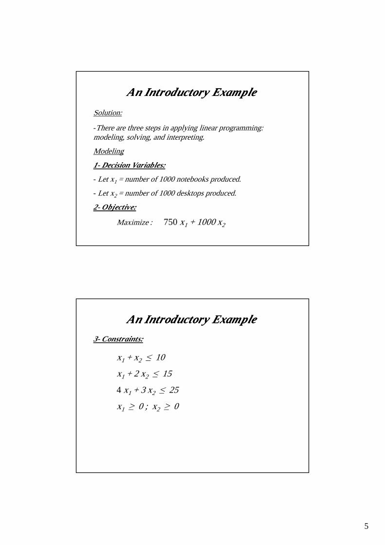
An Introductory ExampleAn Introductory Example
Solution:
-There are three steps in applying linear programming: modeling, solving, and interpreting.
Modeling
1- Decision Variables:
- Let x1 = number of 1000 notebooks produced.
- Let x2 = number of 1000 desktops produced.
2- Objective:
Maximize : 750 x1 + 1000 x2
An Introductory ExampleAn Introductory Example
3- Constraints:
x1 + x2 ≤ 10
x1 + 2 x2 ≤ 15
4 x1 + 3 x2 ≤ 25
x1 ≥ 0 ; x2 ≥ 0

6
Standard Form of Linear ModelStandard Form of Linear Model� There Linear models always have a set of resources
(constraints), m, to produce, n, activities (variables).
� Assume:� Z= value of overall measure of performance� xj = level of activity j (j=1, 2, ….. , n)� cj = increase in Z that result from each unit increase in
activity j� bi = amount of resource i that is available to activity j
(i=1, 2,…, m)� aij = amount of resource i consumed by each unit of
activity j
Standard Form of Linear ModelStandard Form of Linear Model� The general form of allocating resources to activities in
order to form the mathematical linear model is as follows :
ResourceResources usage per unit of activity
1 2 …… nAmount of resource
available
12.
m
a11 a12 …… a1na21 a22 …… a2n…. .... …… …am1 am2 ..….. amn
b1b2…bm
Contribution to Z c1 c2 ……. cn

7
Standard Form of Linear ModelStandard Form of Linear Model
� Maximize Z = c1x1 + c2x2 + …… + cnxn
� Subject to a11x1 + a12x2 + …… + a1nxn ≤ b1
a21x1 + a22x2 + …… + a2nxn ≤ b2
am1x1 + am2x2 + …… + amnxn ≤ bm
and x1 ≥ 0, x2 ≥ 0, ….. xn ≥ 0 non-negativity constraint
Resource Resources usage per unit of activity1 2 …… n
Amount of resource available
12.
m
a11 a12 …… a1na21 a22 …… a2n…. .... …… …am1 am2 ..….. amn
b1b2…bm
Contribution to Z c1 c2 ……. cn
Examples on ModelingExamples on ModelingExample:A company makes two products (X and Y) using two machines (A and B). Each unit of X that is produced requires 50 minutes processing time on machine A and 30 minutes time on machine B. Each unit of Y that is produced requires 24 minutes processing time on machine A and 33 minutes time on machine B.At the start of the current week there are 30 units of X and 90 units of Y in stock. Available processing time on machine A is 40 hours and on machine B is 35 hours. The demand for X in the current week is 75 units and for Y is 95 units. Company policy is to maximize the combined sum of the units of X and the units of Y in stock at the end of the week.
Formulate the problem as a linear program.

8
Examples on ModelingExamples on Modeling
ResourcesActivities
LimitsProduct X Product Y
Machine A time 50 24 40 x 60Machine B time 30 33 35 x 60Units needed X 1 - 75 (30 in stock)Units needed Y - 1 95 (90 in stock)
Contribution to Z 1 1
Examples on ModelingExamples on ModelingThe variables: x: number of units of X produced in the current week y: number of units of Y produced in the current week The constraints: 50x + 24y ≤ 40(60) machine A time 30x + 33y ≤ 35(60) machine B time x ≥ 75 – 30; i.e. x ≥ 45 y ≥ 95 – 90; i.e. y ≥ 5 The objective: Maximize (x+30-75) + (y+90-95) = (x+y-50); i.e. to maximize the number of units left in stock at the end of the week.

9
Examples on ModelingExamples on ModelingExample:A company manufactures two products (A and B) and the profit per unit sold is LE3 and LE5 respectively. Each product has to be assembled on a particular machine, each unit of product A taking 12 minutes of assembly time and each unit of product B 25 minutes of assembly time. The company estimates that the machine used for assembly has an effective working week of only 30 hours.
Technological constraints mean that for every five units of product A produced at least two units of product B must be produced.
Formulate the problem as a linear program.
Examples on ModelingExamples on Modeling
ResourcesActivities
LimitsProduct A Product B
Time 50 24 30 x 60Ratio A:B 5 2 -
Contribution to Z 3 5

10
Examples on ModelingExamples on ModelingThe variables: xA = number of units of A producedxB = number of units of B produced
The constraints: 12 xA + 25xB ≤ 30(60) (assembly time)xB ≥ 2(xA /5); i.e. xB - 0.4 xA ≥ 0; i.e. 5 xB ≥ 2 xAxA, xB ≥ 0
The objective: maximize 3 xA + 5 xb
Examples on ModelingExamples on ModelingExample: An aggregate mixture contains a minimum of 30% sand and no more than 60% gravel nor 10% silt. Three sources of aggregate are available: pit 1, pit 2 and pit 3 as shown in the table. A total mix of at least 10,000 m3 is required. With the objective to minimize the cost of material, Define the decision variables and Formulate a mathematical model
Pit 1 2 3
% Sand% Gravel
% SiltCost/m3
56035
LE 2
3070-
LE 10
100--
LE 8
11
Examples on ModelingExamples on Modeling
ResourcesActivities
LimitsPit 1 (x1) Pit 2 (x2) Pit 3 (x3)
Total aggregate required
1 1 1 10000
Sand % 0.05 0.3 1 3000Gravel % 0.6 0.7 - 6000
Silt % 0.35 - - 1000Contribution to Z 2 10 8
Examples on ModelingExamples on ModelingThe variables: x1 = amount of aggregate from pit 1x2 = amount of aggregate from pit 2 x3 = amount of aggregate from pit 3The constraints: Total amount of aggregate required = 10000 m3x1 + x2 + x3 ≥ 10000Amount of sand not less than 30% = 0.3 x 10000 = 3000 m30.05 x1 + 0.3 x2 + x3 ≥ 3000Amount of gravel not more than 60% = 0.6 x10000 = 6000 m30.6 x1 + 0.7 x2 ≤ 6000Amount of silt not more than 10% = 0.1 x 10000 = 1000 m30.35 x1 ≤ 1000; x1, x2, x3 ≥ 0The objective: Minimize 2 x1 + 10 x2 + 8 x3

12
An Introductory ExampleAn Introductory Example
Solving the Model Graphically
1- Plotting the constraints to bound the feasible region
An Introductory ExampleAn Introductory Example
Solving the Model Graphically
2- Finding optimal solution

13
An Introductory ExampleAn Introductory Example
Solving the Model Graphical ly
3- Terminology of the Model Solution
An Introductory ExampleAn Introductory Example
An optimal solutionis a feasible solution that has the most
favorable value of the objective function.
A corner-point feasible (CPF) solutionis a solution that lies
at a corner of the feasibleregion.
Active constraintis the constraint that share in forming the
feasible region.
In-active constraintis the constraint that doesn’t share informing the feasible region.
14
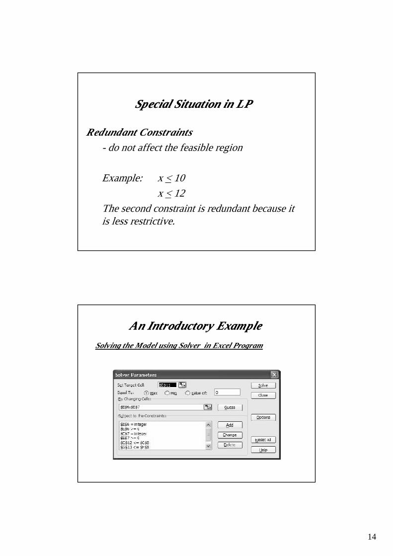
Special Situation in LPSpecial Situation in LP
Redundant Constraints - do not affect the feasible region
Example: x <10x < 12
The second constraint is redundant because it is less restrictive.
An Introductory ExampleAn Introductory Example
Solving the Model using Solver in Excel Program

15
Types of SolutionsTypes of Solutions1. Unique Optima– when one optimum solution exists
Max total weekly profit, Z = 140x1 + 160x2
Subject to: 2x1 + 4x2 ≤ 285x1 + 5x2 ≤ 50x1 ≤ 8x2 ≤ 6x1, x2 ≥ 0
Feasible region
x1 ≤ 8
1480 = 140x1 + 160x2
2x1 + 4x2 ≤ 28
5x1 + 5x2 ≤ 50
x2 ≤ 6
(6, 4) Unique optimal solution
Types of SolutionsTypes of Solutions2. Alternate Optimal Solutions– when there is more
than one optimal solution
Max 2T + 2CSubject to:
T + C < 10T < 5
C < 6T, C > 0
0 5 10 T
C
10
6
All points onRed segment are optimal

16
Types of SolutionsTypes of Solutions3. Infeasibility – when no feasible solution exists (there
is no feasible region)Example: x <10
x > 15
5x1 + 5x2 ≤ 50x1 ≥ 8x2 ≥ 6
Types of SolutionsTypes of Solutions
4. Unbounded Solutions – when nothing prevents the solution from becoming infinitely large
Max 2T + 2CSubject to:
2T + 3C > 6T, C > 0
0 1 2 3 T
C
2
1
0
17
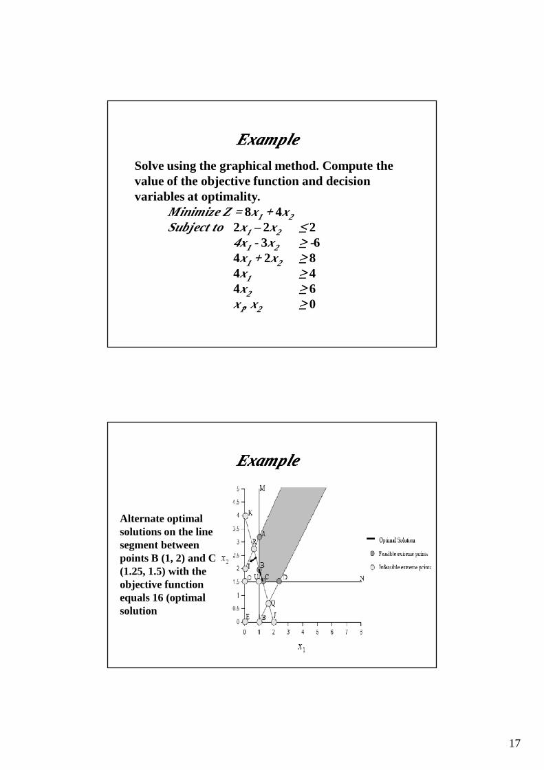
ExampleExample
Solve using the graphical method. Compute the value of the objective function and decision variables at optimality.
Minimize Z = 8x1 + 4x2Subject to 2x1 – 2x2 ≤ 2
4x1 - 3x2 ≥ -64x1 + 2x2 ≥ 84x1 ≥ 44x2 ≥ 6x1, x2 ≥ 0
ExampleExample
Alternate optimal solutions on the line segment between points B (1, 2) and C (1.25, 1.5) with the objective function equals 16 (optimal solution

18
Example Example 22- A marketing company is planning a one week advertising
campaign for their new knife. The ads have been designed
and produced and now they wish to determine how much
money to spend in each advertising outlet. They have
hundreds of possible outlets to choose from. Let’s
consider two outlets: Prime-time TV, and newsmagazines.
The problem of optimally spending advertising money can
be formulated in many ways. For instance, given a fixed
budget, the goal might be to maximize the number of
target customers reached (customer with a reasonable
chance of purchasing the product).
Example Example 2 2 (continue)(continue)- An alternative approach, which we adopt here, is to define
targets for reaching each market segment and to minimize
the money spent to reach those targets. For this product,
the target segments are teenage boys, women (ages 40-49),
and retired men. Each minute of primetime TV and page
of newsmagazine advertisement reaches the following
number of people (in millions):
19
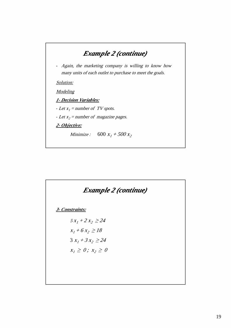
- Again, the marketing company is willing to know how
many units of each outlet to purchase to meet the goals.
Solution:
Modeling
1- Decision Variables:
- Let x1 = number of TV spots.
- Let x2 = number of magazine pages.
2- Objective:
Minimize : 600 x1 + 500 x2
Example Example 2 2 (continue)(continue)
3- Constraints:
5 x1 + 2 x2 ≥ 24
x1 + 6 x2 ≥ 18
3 x1 + 3 x2 ≥ 24
x1 ≥ 0 ; x2 ≥ 0
Example Example 2 2 (continue)(continue)

20
Solving the Model Graphical ly
Example Example 2 2 (continue)(continue)
Solving the Model using Solver in Excel Program
Example Example 2 2 (continue)(continue)

21
Proportionality Assumption
Limitations of LP ModelingLimitations of LP Modeling
Since the objective is linear, the contribution to the objective of any decision variable is proportional to the value of the decision variable.
Additivity Assumption
Since each constraint is linear, the contribution of each variable to the left hand side of each constraint is proportional to the value of the variable and independent of the values of any other variable
Divisibility Assumption
Limitations of LP ModelingLimitations of LP Modeling
When it is impossible to take a fraction of the decision variable, then the used value violates the optimality.
Certainty Assumption
It is very rare that a problem will meet all of the assumptions exactly. A model can still give useful managerial insight even if reality differs slightly from the rigorous requirements of the model.