main linac beam dynamics - linear collider collaboration · main linac beam dynamics kiyoshi kubo...
TRANSCRIPT
Main Linac Beam Dynamics
Kiyoshi KUBO2006.05.22
(Some slides will be skipped in the lecture, due to the limited time.)

ILC Main Linac Beam Dynamics
• Introduction • Lattice design• Beam quality preservation
– Longitudinal – Transverse
• Wakefield– Single bunch, Multi-bunch– BBU, Cavity misalignment
• Dispersive effect– Errors and corrections
• Initial alignment, fixed errors• Vibration, ground motion, jitters, etc.
Note• The hard copy is from very old version, having a lot of
mistakes. Please look at the latest version.• Basics will not be lectured here.
– Beam optics: What are Emittance, Beta-function, Dispersion function, etc..
– Wakefield: Definition of wake-function, etc..(See lectures yesterday.)
• Numbers quoted here and simulation results shown here may be preliminary.
About Home Work
• There are five exercises– Shown as “HMWK-1”, “HMWK-2”, , ,
“HMWK-5” in the slides• Choose at least one.
– two, if possible.

Introduction• Main Linac is very simple, compare with most of
other part of LC. – Basically many iteration of a simple unit.
• Some statistical calculations are useful because of the large number of identical components.
• Still, analytical treatment is very limited. And most studies are based on simulations.– Even in simulations, approximations are necessary for
reasonable calculation time.• e.g., 2E10 particles cannot be simulated individually.
Detailed treatment of edge fields of magnets and cavities may not be necessary. Space charge can be ignored for high energy beams.
• “What can be ignored?” is important in simulation.
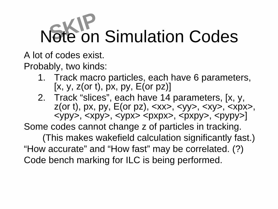
A lot of codes exist.Probably, two kinds:
1. Track macro particles, each have 6 parameters, [x, y, z(or t), px, py, E(or pz)]
2. Track “slices”, each have 14 parameters, [x, y, z(or t), px, py, E(or pz), <xx>, <yy>, <xy>, <xpx>, <ypy>, <xpy>, <ypx> <pxpx>, <pxpy>, <pypy>]
Some codes cannot change z of particles in tracking.(This makes wakefield calculation significantly fast.)
“How accurate” and “How fast” may be correlated. (?)Code bench marking for ILC is being performed.
SKIPNote on Simulation Codes

Parameter of ILC Main Linac(ECM=500 GeV)
Beam energy 13~15 GeV to 250 GeV
Acc. gradient 31.5 MV/m
Bunch Population 1 ~ 2 x10¹⁰ /bunch
Number of bunches <= 5640 /pulse
Total particles <=5.64 x10¹³ /pulse
Bunch spacing >= 150 ns
Bunch Length 0.15 ~ 0.3 mm
Emittance x (at DR exit/IP)
Emittance y (at DR exit/IP)
8/10~12 x10-6 m-rad2/3~8 x10-8 m-rad
Lattice design
• Basic layout– One quad per four cryomodules
• May be changed to one quad/three modules– Simple FODO cell
x/y = 75/65 degree phase advance/cellOther possible configurations: change along linac
• Higher the energy, larger the beta-function• FOFODODO, FOFOFODODODO, etc., in high
energy region• Vertically curved, following the earth curvature

Unit of main linacabout 240 units/linac
Cryomodule with magnet package
Cryomodules without magnet package
9-cell SC cavity
Magnet package
BPM
Quadrupole SC magnetDipole SC magnet
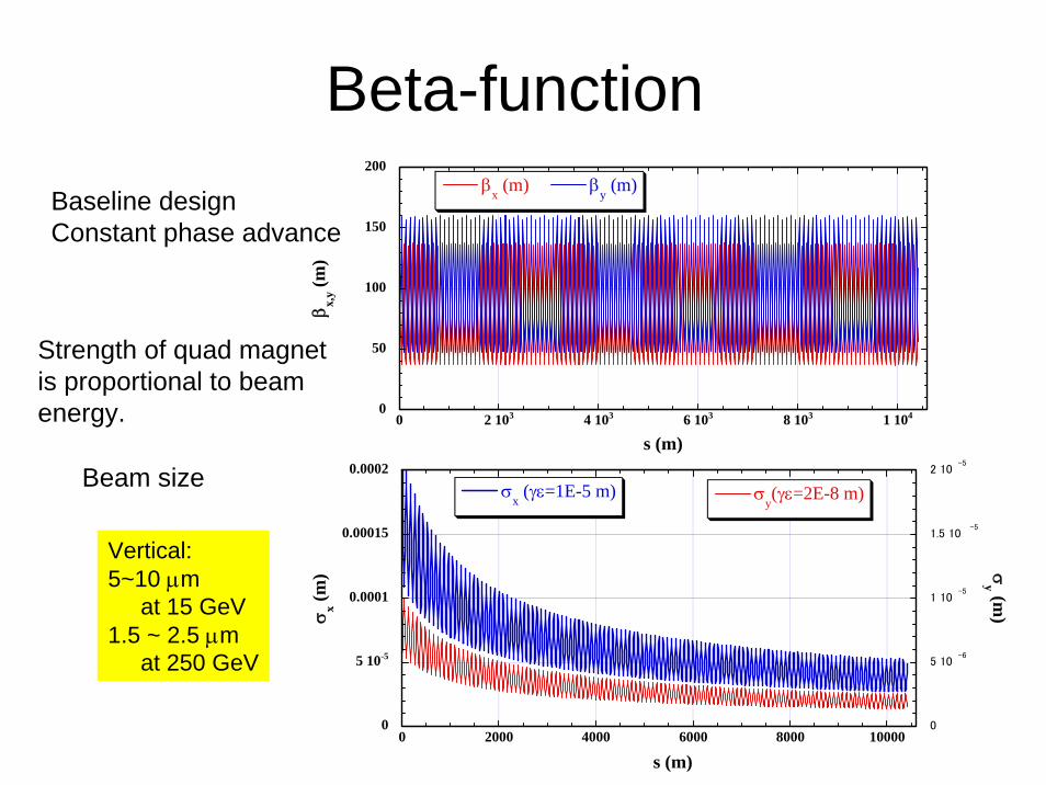
Beta-function
0
50
100
150
200
0 2 103 4 103 6 103 8 103 1 104
βx (m) β
y (m)
β x,y (m
)
s (m)
Baseline designConstant phase advance
Beam size
0
5 10-5
0.0001
0.00015
0.0002
0
5 10-6
1 10-5
1.5 10-5
2 10-5
0 2000 4000 6000 8000 10000
σx (γε=1E-5 m) σ
y(γε=2E-8 m)
σ x (m) σ
y (m)
s (m)
Vertical:5~10 μm
at 15 GeV1.5 ~ 2.5 μm
at 250 GeV
Strength of quad magnet is proportional to beam energy.
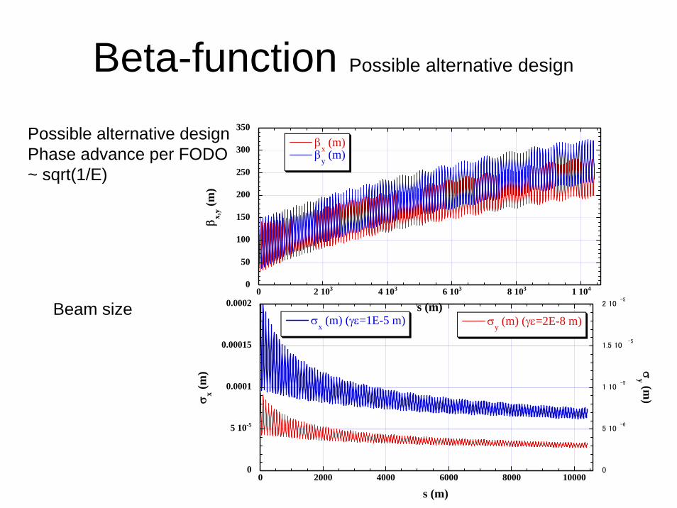
Beta-function Possible alternative design
0
50
100
150
200
250
300
350
0 2 103 4 103 6 103 8 103 1 104
βx (m)
βy (m)
β x,y (m
)
s (m)
Possible alternative designPhase advance per FODO ~ sqrt(1/E)
0
5 10-5
0.0001
0.00015
0.0002
0
5 10-6
1 10-5
1.5 10-5
2 10-5
0 2000 4000 6000 8000 10000
σx (m) (γε=1E-5 m) σ
y (m) (γε=2E-8 m)
σ x (m) σ
y (m)
s (m)
Beam size
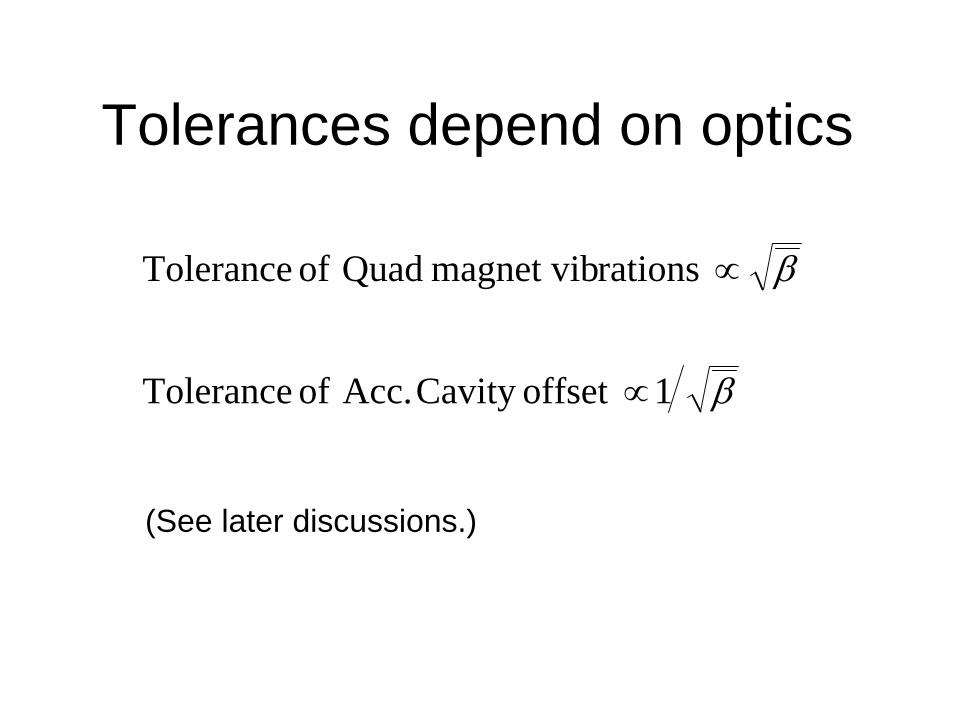
Tolerances depend on optics
β
β
1offset Cavity Acc. of Tolerance
rationsmagnet vib Quad of Tolerance
∝
∝
(See later discussions.)
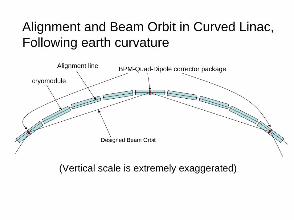
BPM-Quad-Dipole corrector packageAlignment line
Designed Beam Orbit
Alignment and Beam Orbit in Curved Linac,Following earth curvature
(Vertical scale is extremely exaggerated)
cryomodule
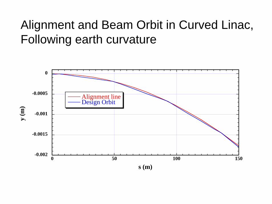
-0.002
-0.0015
-0.001
-0.0005
0
0 50 100 150
Alignment lineDesign Orbit
y (m
)
s (m)
Alignment and Beam Orbit in Curved Linac,Following earth curvature
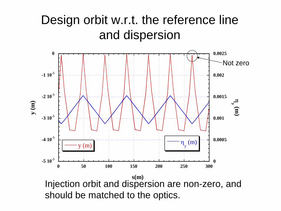
Design orbit w.r.t. the reference line and dispersion
Injection orbit and dispersion are non-zero, and should be matched to the optics.
Not zero
-5 10-5
-4 10-5
-3 10-5
-2 10-5
-1 10-5
0
0
0.0005
0.001
0.0015
0.002
0.0025
0 50 100 150 200 250 300
y (m) ηy (m)
y (m
) ηy (m
)
s(m)

Beam Quality Preservation

Beam Quality• Longitudinal particle distribution
– Energy and arriving time, or longitudinal position• E and t, or z
• Transverse particle distribution– Horizontal and vertical position and angle
• x, x’, y, y’ (or x, px, y, py)Generally, “Stable and small distributions at IP”is preferable.
Exception:x and z distribution at IP should not be too small.( beam-beam interaction)
Longitudinal Beam Quality

Longitudinal beam quality• Beam energy stability• Small energy spread.These require RF amplitude and phase stability,
which rely on RF control.The stability requirement in main linacs is less
severe than in bunch compressors.
Main Linac does (almost) nothing to the timing and bunch length.
( Bunch Compressor)
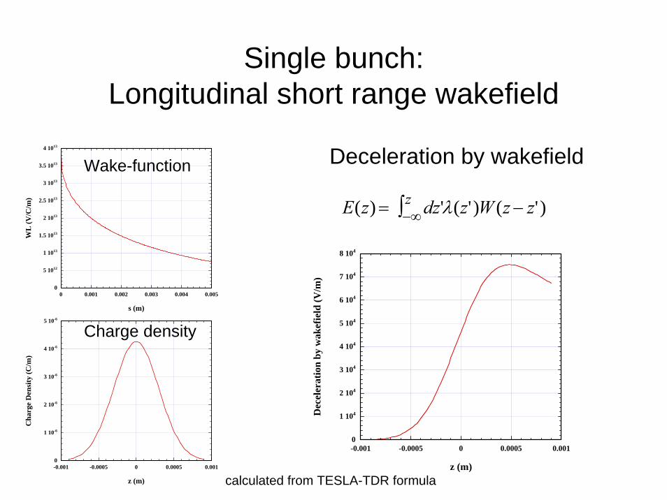
Single bunch: Longitudinal short range wakefield
0
5 1012
1 1013
1.5 1013
2 1013
2.5 1013
3 1013
3.5 1013
4 1013
0 0.001 0.002 0.003 0.004 0.005
WL
(V/C
/m)
s (m)
Wake-function
0
1 10-6
2 10-6
3 10-6
4 10-6
5 10-6
-0.001 -0.0005 0 0.0005 0.001
Cha
rge
Den
sity
(C/m
)
z (m)
E(z) = dz'−∞z∫ λ(z' )W (z − z' )
Charge density
Deceleration by wakefield
0
1 104
2 104
3 104
4 104
5 104
6 104
7 104
8 104
-0.001 -0.0005 0 0.0005 0.001
Dec
eler
atio
n by
wak
efie
ld (V
/m)
z (m)calculated from TESLA-TDR formula

Total acceleration (RF off-crest phase 4.6 deg. minimizing energy spread.)
3.125 107
3.13 107
3.135 107
3.14 107
3.145 107
0
5 104
1 105
1.5 105
2 105
-0.001 -0.0005 0 0.0005 0.001
RF fieldTotal acceleration
wakefield Acc
eler
atin
g fie
ld (V
/m)
wakefield (V
/m)
z (m)
Energy spread along linac. Initial spread is dominant.
1.5 108
1.52 108
1.54 108
1.56 108
1.58 108
1.6 108
0 5 1010 1 1011 1.5 1011 2 1011 2.5 1011
Positron
σ E (e
V)
E (eV)
0
0.002
0.004
0.006
0.008
0.01
0.012
0 5 1010 1 1011 1.5 1011 2 1011 2.5 1011
Positron
Electron
σ E/E
E (eV)
Undulator for e+ source
Bunch by bunch energy difference
• Should be (much) smaller than single bunch energy spread
• Accurate RF control will be essential – Compensation of beam loading– Compensation of Lorentz detuning
• Longitudinal higher order mode wakefield will not be a problem.
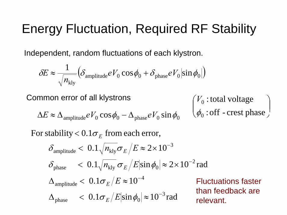
Energy Fluctuation, Required RF Stability
Common error of all klystrons
00phase00amplitude sincos φφ eVeVE Δ−Δ≈Δ
( )00phase00amplitudekly
sincos1 φδφδδ eVeVn
E +≈
Independent, random fluctuations of each klystron.
rad10sin1.0
101.0
rad102sin1.0
1021.0
error,each from 1.0stability For
30phase
4amplitude
20klyphase
3klyamplitude
−
−
−
−
≈<Δ
≈<Δ
×≈<
×≈<
<
φσ
σ
φσδ
σδ
σ
E
E
En
En
E
E
E
E
E
⎟⎟⎠
⎞⎜⎜⎝
⎛phasecrest -off :
voltage total:
0
0
φV
Fluctuations faster than feedback are relevant.
Transverse Motion

Transverse beam quality• Beam position at IP
– Offset between two beams should be (much) smaller than the beam size
• Beam size at IP, Emittance– From consideration of beam-beam interaction, ‘flat’
beam is desirable.• vertical size is much smaller than horizontal size
– Beam size at IP is limited by emittance• Hour glass effect and Oide limit
– Then, vertical emittance need to be very small.• Vertical position stability and vertical emittance
preservation are considered
Beam position jitter
• There will be position feedback in Main Linac, BDS, then, at IP, and feed-forward in RTML (turnaround).
• In Main Linac, only fast jitter (faster than the feedback) should be important, unless it causes emittance dilution.
• The dominant source can be:– vibration of quadrupole magnets.– Strength jitter of quadrupole and dipole magnets
(instability of power supplies)
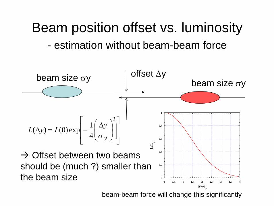
Beam position offset vs. luminosity- estimation without beam-beam force
offset Δybeam size σy beam size σy
⎥⎥
⎦
⎤
⎢⎢
⎣
⎡
⎟⎟⎠
⎞⎜⎜⎝
⎛ Δ−=Δ
2
41exp)0()(
y
yLyLσ
Offset between two beams should be (much ?) smaller than the beam size 0
0.2
0.4
0.6
0.8
1
0 0.5 1 1.5 2 2.5 3 3.5 4
L/L
0
Δy/σy
beam-beam force will change this significantly

Estimation of beam position change due to quad offset change
Final beam position is sum of all quads’ contribution. Assuming random, independent offset, expected beam position offset is:
4/sin 22222 kNaEEky fqquad
fiiiiff ββϕββ ≈>≈< ∑
iiffiiif EEkay ϕββ sin/−=ΔFinal position change due to offset of i-th quad:
final toquadth - from cephaseadvan:
onbetafuncti final : quad,th -at on betafuncti :
value,-k:energy beam final : quad,th -at energy beam :quad,th - of )( value-k: quad,th - ofoffset : 1
i
i
kEiEifkia
i
fi
ifi
-ii
ϕ
ββ
square value-k of average: on,betafuncti of average:
quads, ofnumber : offset, of rms:2k
Na q
β
Please confirm or confute expressions in this page.
HMWK-1
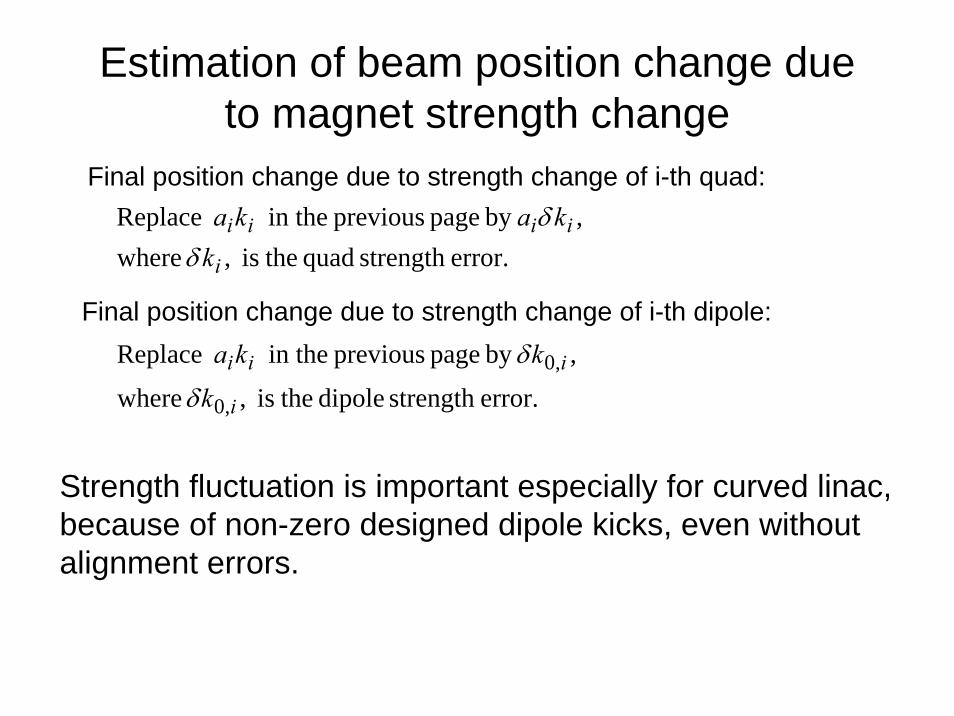
Estimation of beam position change due to magnet strength change
error.strength quad theis , where,by pagepreviousin the Replace
i
iiiik
kakaδ
δFinal position change due to strength change of i-th quad:
error.strength dipole theis , where
,by page previous in the Replace
,0
,0
i
iii
k
kka
δ
δFinal position change due to strength change of i-th dipole:
Strength fluctuation is important especially for curved linac, because of non-zero designed dipole kicks, even without alignment errors.

Stronger focus optics make quad vibration tolerance tighter
βεβε
ββ
σ y
q
fy
fq
y
f NakNay~
222=≈
><
Beam position jitter / beam size:
proportional to:quad vibrationsquare root of number of quads
inversely proportional to:square root of average beta-functionsquare root of emittance
Beam quality - Emittance• Our goal is high luminosity• For (nearly) Gaussian distribution,
emittance is a good measure of luminosity– We are usually interested in this case.
• But, . . . . .• We use emittance dilution as a measure of
quality dilution in the main linac, anyways.
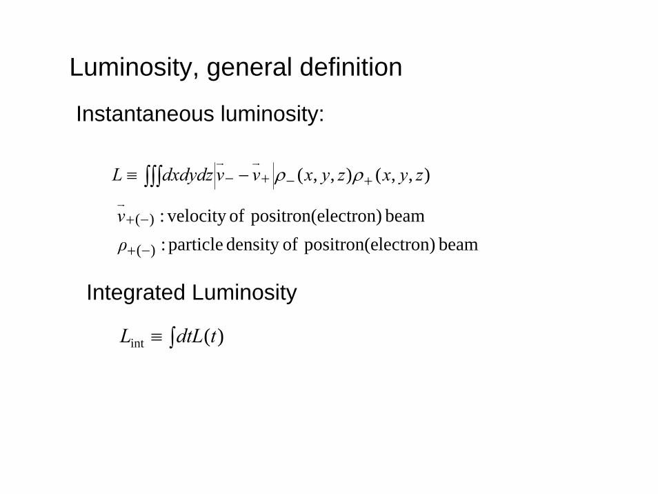
∫∫∫ +−+− −≡ ),,(),,( zyxzyxvvdxdydzL ρρ
Luminosity, general definition
beam lectron)positron(e ofdensity particle :beam lectron)positron(e of velocity :
)(
)(
−+
−+
ρv
Instantaneous luminosity:
∫≡ )(int tdtLL
Integrated Luminosity

Luminosity per bunch crossing for Gaussian beamhead on collision, no de-formation due to beam-beam force
2,
2,
2,
2,2 yyxx
NN
+−+−
+−
++=
σσσσπ
⎟⎟⎠
⎞⎜⎜⎝
⎛ +−−∝⎟
⎟⎠
⎞⎜⎜⎝
⎛−∝
+−+−
+−+−
zz
yxyx
ctzyx),(
2
),()(),(
22
)(),( 2))((exp,
2)(exp
σλ
σλ
∫ ∫∫ ∫ +−+−+−+−= yyxxzzbc dydxNcNdzdtL ,,,,,,2 λλλλλλ
zyxNzyx λλλρ =),,(
If e+ and e- beams are the same size, luminosity is proportional to inverse of beam’s cross section.
: density per volume
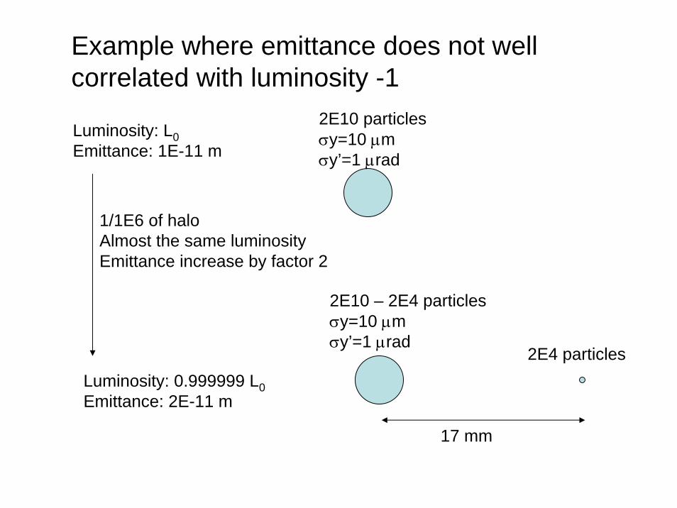
2E10 particlesσy=10 μmσy’=1 μrad
Luminosity: L0Emittance: 1E-11 m
2E10 – 2E4 particlesσy=10 μmσy’=1 μrad
17 mm
2E4 particlesLuminosity: 0.999999 L0Emittance: 2E-11 m
1/1E6 of haloAlmost the same luminosityEmittance increase by factor 2
Example where emittance does not well correlated with luminosity -1

Example where emittance does not well correlated with luminosity -2
So called “banana effect”
Same projected emittance.Different luminosity
Beam-beam interaction
z-y correlated
no correlation

NOTE• We use emittance as a measure of quality in
the main linac.• Halos, tails far from core should be ignored in
calculating the emittance.– Effects of halos or tails should be considered in
other context.• Luminosity may not be well correlated to emittance, in
some cases, because of Beam-beam force at IP• Does any parameter represent luminosity better than
emittance, which can be evaluated without collision simulations? HMWK-2

Dominant Sources oftransverse Emittance dilution
• Wakefield (transverse) of accelerating cavities– Electromagnetic fields induced by head
particles affect following bunches.• z-correlated orbit difference
• Dispersive effect– Different energy particles change different
angles by electromagnetic fields (designed or not-designed). • energy correlated orbit difference

Effects of Transverse Wakefield

Transverse Wakefield ofAccelerating cavities
• Short range - Single bunch effect– Wakefunction is monotonic function of distance– Not seriously important for ILC
• Long range - Multi-bunch effect– Many higher order oscillating mode– For ILC
• Need to be damped• Frequency spread is needed. (may naturally
exist ?)• Need to be careful for x-y coupling
• BBU [Beam Break Up] (injection error)• Effect of cavity misalignment
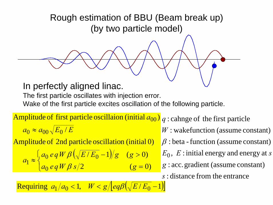
Rough estimation of BBU (Beam break up)(by two particle model)
In perfectly aligned linac.The first particle oscillates with injection error.Wake of the first particle excites oscillation of the following particle.
entrancethefromdistance:constant) (assumegradient acc.:
atenergy andenergy initial:, constant) (assumefunction -beta: constant) (assumeon wakefuncti:
particlefirst theofcahnge:
0
sg
sEE
Wq
β
( )⎩⎨⎧
=
>−≈
≈
)0(2)0(1/
)0 (initialn oscillatio particle 2nd of Amplitude/
)(initialoscillaionparticlefirst of Amplitude
0
001
0000
00
gsWqeaggEEWqea
a
EEaa
a
ββ
( )[ ]1/,1 Requiring 001 −<< EEeqgWaa β
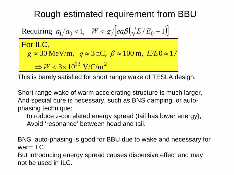
Rough estimated requirement from BBU
( )[ ]1/,1 Requiring 001 −<< EEeqgWaa β
213 V/C/m103
170 m, 100 nC,3 MeV/m, 30
×<⇒
≈≈≈≈
W
E/Eqg βFor ILC,
This is barely satisfied for short range wake of TESLA design.
Short range wake of warm accelerating structure is much larger.And special cure is necessary, such as BNS damping, or auto-phasing technique:
Introduce z-correlated energy spread (tail has lower energy),Avoid ‘resonance’ between head and tail.
BNS, auto-phasing is good for BBU due to wake and necessary for warm LC.But introducing energy spread causes dispersive effect and may not be used in ILC.
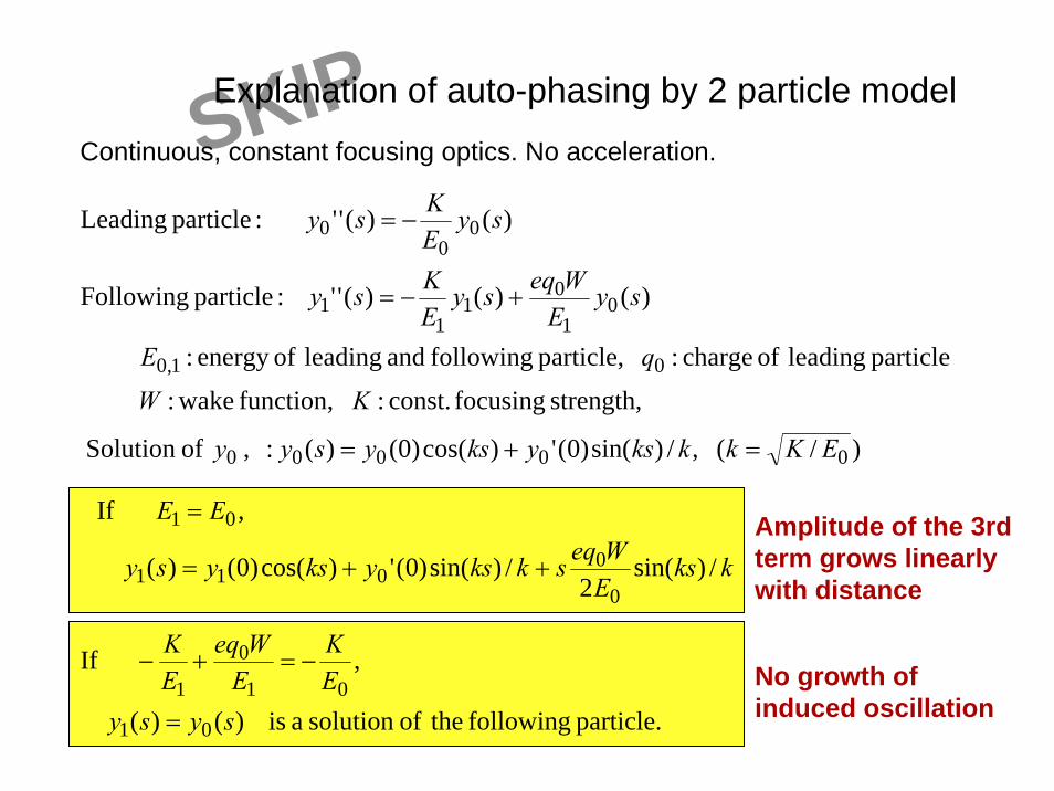
strength, focusing const.: function, wake:
particle leading of charge: particle, following and leading ofenergy :
)()()('' :particle Following
)()('' :particle Leading
01,0
01
01
11
00
0
KW
qE
syE
WeqsyEKsy
syEKsy
+−=
−=
)/( ,/)sin()0(')cos()0()(: , ofSolution 00000 EKkkksyksysyy =+=
Amplitude of the 3rd term grows linearly with distance
No growth of induced oscillation
kksEWeqskksyksysy
EE
/)sin(2
/)sin()0(')cos()0()(
, If
0
0011
01
++=
=
particle. following theofsolution a is )()(
, If
01
01
0
1
sysyEK
EWeq
EK
=
−=+−
SKIPExplanation of auto-phasing by 2 particle modelContinuous, constant focusing optics. No acceleration.
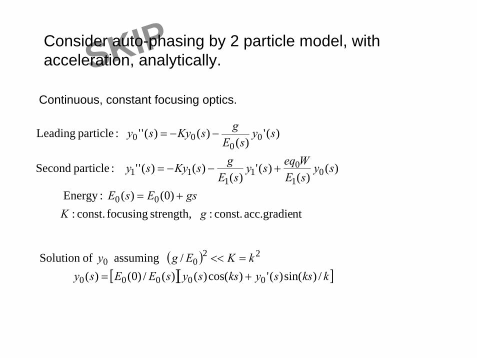
Continuous, constant focusing optics.
ntacc.gradie const.: strength, focusing const.: )0()( :Energy
)()(
)(')(
)()('' :particle Second
)(')(
)()('' :particle Leading
00
01
01
111
00
00
gKgsEsE
sysEWeqsy
sEgsKysy
sysE
gsKysy
+=
+−−=
−−=
( )[ ][ ]kkssykssysEEsy
kKEgy/)sin()(')cos()()(/)0()(
/ assuming ofSolution
00000
2200
+==<<
SKIPConsider auto-phasing by 2 particle model, with acceleration, analytically.

-15
-10
-5
0
5
10
15
0 50 100 150 200 250 300
0.1ΔEauto
-15
-10
-5
0
5
10
15
0 50 100 150 200 250 300
ΔEauto
-15
-10
-5
0
5
10
15
0 50 100 150 200 250 300
1.5ΔEauto
Oscillation piriod of the leeding bunch
-30
-20
-10
0
10
20
30
0 50 100 150 200 250 300
ΔE=0
-15
-10
-5
0
5
10
15
0 50 100 150 200 250 300
0.5ΔEauto
SKIPOscillation of second particle.Two particle model.No acceleration
Unit of the amplitude of the leading particle .
No energy difference: Amplitude grows linearly.
Auto-phasing:Oscillate as same as the leading particle.
More energy difference:BNS Damping
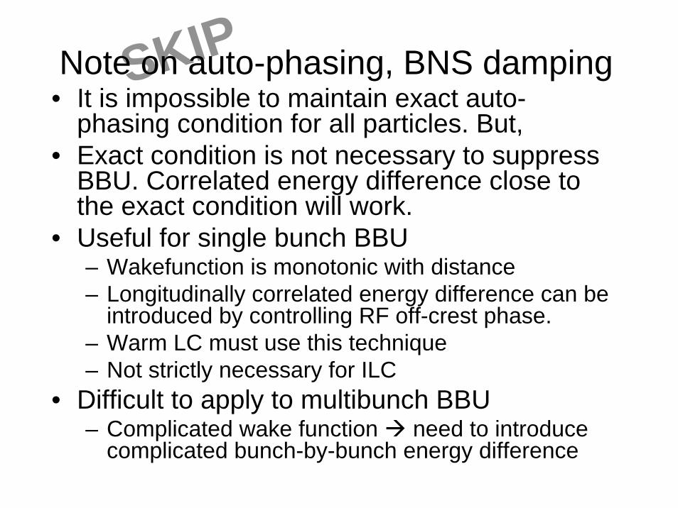
• It is impossible to maintain exact auto-phasing condition for all particles. But,
• Exact condition is not necessary to suppress BBU. Correlated energy difference close to the exact condition will work.
• Useful for single bunch BBU– Wakefunction is monotonic with distance– Longitudinally correlated energy difference can be
introduced by controlling RF off-crest phase.– Warm LC must use this technique– Not strictly necessary for ILC
• Difficult to apply to multibunch BBU– Complicated wake function need to introduce
complicated bunch-by-bunch energy difference
SKIPNote on auto-phasing, BNS damping
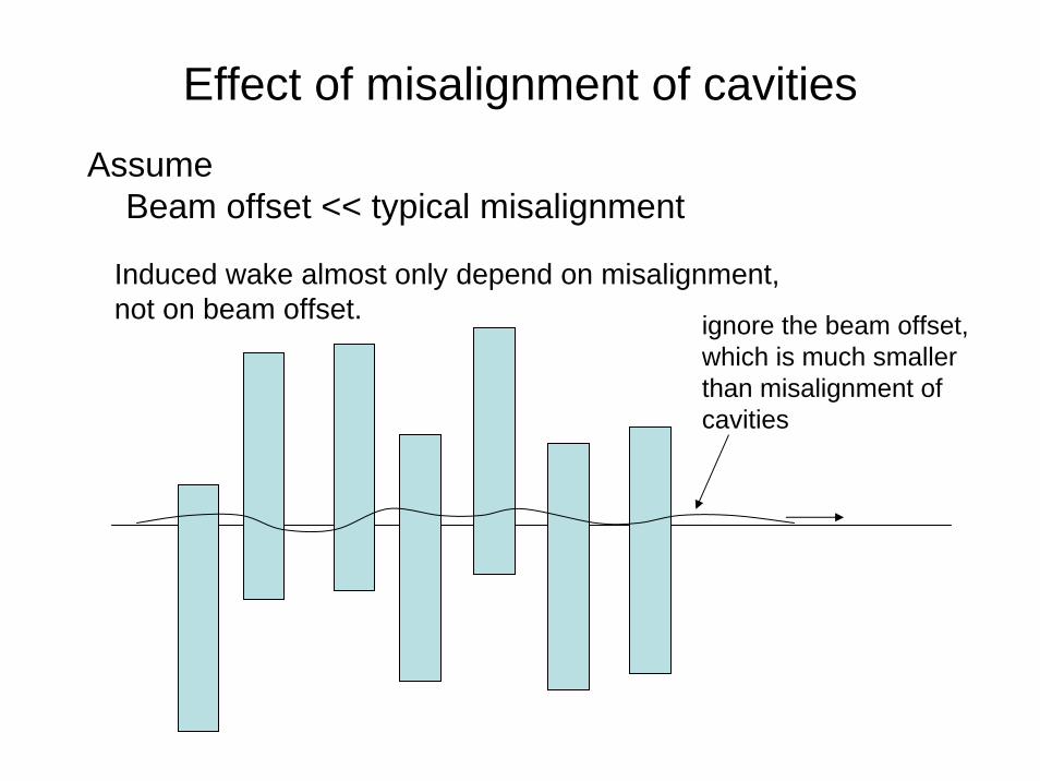
Effect of misalignment of cavitiesAssume
Beam offset << typical misalignment
Induced wake almost only depend on misalignment,not on beam offset. ignore the beam offset,
which is much smaller than misalignment of cavities

Effect of misalignment of cavities-continued
∑−=i
iiffiijifj EEWaey ϕββ sin/1,,
f
fjfcav
iiifij
fiifj gE
EEWLaeW
EEeay
2)/log(
sin 0222
22,
222
,ββ
ϕββ ≈><>=< ∑
)( :wake"- sum" , kjjk
ikij zzWqW −= ∑<
Position change of j-th particle at linac end due to i-th cavity:
Expected Position change square of j-th particle:
gradient, acc.: length,cavity : particel,th -k of charge:
final, cavity toth -i from advance phase: beta, final andcavity th -iat beta:,
energy, final andcavity th -iat energy :, cavity,th -iofoffset :
gLq
EEa
cavi
k
i
ii
fi
i
ϕββ
iiffiijifi EEWeay ϕββ sin/1,, −=
Position change at linac end:
Please confirm or confute expressions in this page.
assume all cavities have the same wakefunction
HMWK-3
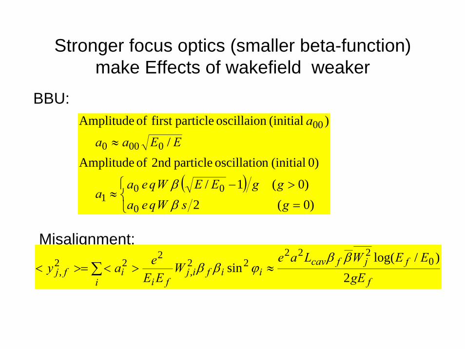
Stronger focus optics (smaller beta-function) make Effects of wakefield weaker
( )⎩⎨⎧
=
>−≈
≈
)0(2)0(1/
)0 (initialn oscillatio particle 2nd of Amplitude/
)(initial oscillaionparticlefirst ofAmplitude
0
001
0000
00
gsWqeaggEEWqea
a
EEaa
a
ββ
BBU:
Misalignment:
f
fjfcav
iiifij
fiifj gE
EEWLaeW
EEeay
2)/log(
sin 0222
22,
222
,ββ
ϕββ ≈><>=< ∑
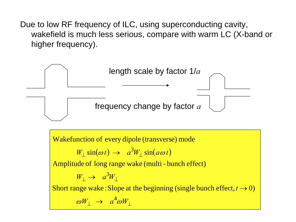
Due to low RF frequency of ILC, using superconducting cavity, wakefield is much less serious, compare with warm LC (X-band or higher frequency).
length scale by factor 1/a
frequency change by factor a
( ) ( )
⊥⊥
⊥⊥
⊥⊥
→
→→
→
WaW
tWaW
taWatW
ωω
ωω
4
3
3
)0 effect,bunch single( beginning at the Slope : wakerangeShort
effect)bunch -(multi wakerange long of Amplitudesinsin
mode e)(transversdipoleevery ofon Wakefuncti

Explanation of Wakefunction Scaling with size
length scaled by factor 1/a
Look at one dipole mode (justified by principle of superposition, for many modes)
)/(ion wakefunctse transverand 2/ on,preservatienergy from then, voltage, theof half one a feels'' change drive The
:gradient Average , :Voltage , :Energy y,offset at cavity ugh thewent throchargedriveaby fielld Exited :cavityLeft
0000
000
LyqV WqVU
EVUq
==
y q y/aq’
0311
01
20
10
3
001
03
)'/(function wakee transversand
'2/'
on,preservatienergy From:gradient Average ,:Voltage , :Energy
scaled)(length on distributi field same thegradient,sametheexited offset ugh went thro'chargedriveA :cavityRight
WaLaqyaV a
qaqVaqUa
E V aUa
y/aq
-
-
==
=⇒=−−−
−−
−
cavity length Lcavity length L/a
Please confirm or confute expressions in this page.
HMWK-4
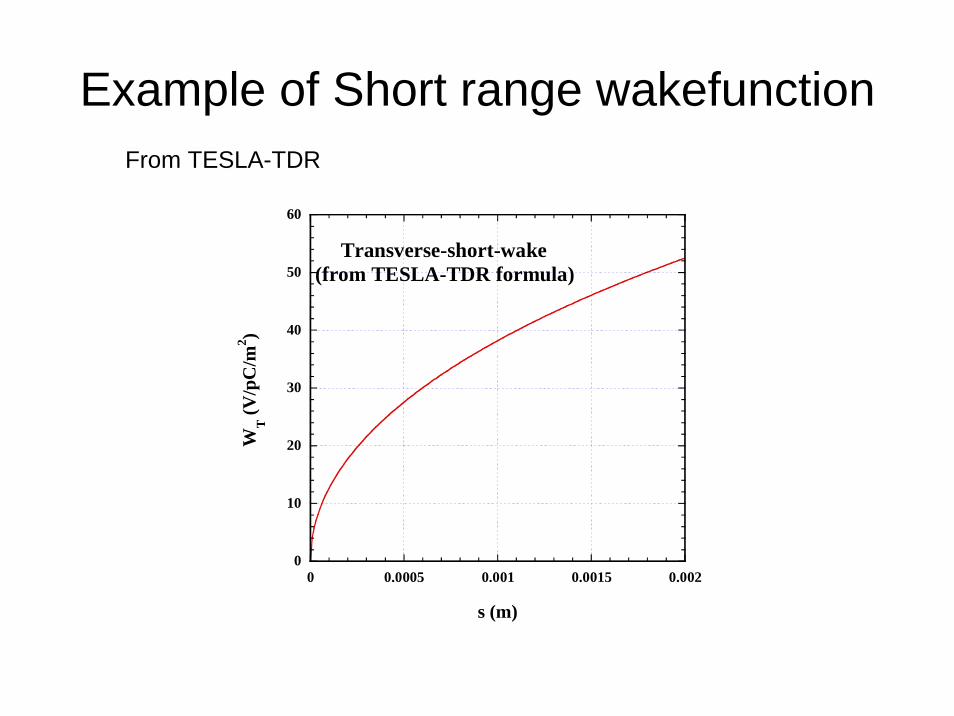
Example of Short range wakefunctionFrom TESLA-TDR
0
10
20
30
40
50
60
0 0.0005 0.001 0.0015 0.002
Transverse-short-wake(from TESLA-TDR formula)
WT (V
/pC
/m2 )
s (m)

Example of simulation of short range wake effect-1
Single bunch BBU, with injection offset in perfectly aligned linac.Emittance along linac, injection offset 1 σ of beam size. monochromatic beam.
y-z, y’-z, y’-y distribution at the end of linac
2 10-8
2.005 10-8
2.01 10-8
2.015 10-8
2.02 10-8
2.025 10-8
0 2000 4000 6000 8000 10000
proj
ecte
d γε
(μ)
s (m)
8 10-7
1 10-6
1.2 10-6
1.4 10-6
1.6 10-6
1.8 10-6
-8 10-4 -6 10-4 -4 10-4 -2 10-4 0 100 2 10-4 4 10-4 6 10-4 8 10-4
injection 1 sigma, monochro
y (m
)
z (m)
-5 10-9
0
5 10-9
1 10-8
1.5 10-8
2 10-8
2.5 10-8
-8 10-4 -6 10-4 -4 10-4 -2 10-4 0 100 2 10-4 4 10-4 6 10-4 8 10-4
injection 1 sogma, monochro
y'
z (m)
-5 10-9
0
5 10-9
1 10-8
1.5 10-8
2 10-8
2.5 10-8
8 10-7 1 10-6 1.2 10-6 1.4 10-6 1.6 10-6 1.8 10-6
y'
y (m)

Example of simulation of short range wake effect-2
Single bunch, random misalignment of cavities, sigma=0.5 mm.Emittance along linac. One linac and average of 100 seeds. monochromatic beam.
2 10-8
2.02 10-8
2.04 10-8
2.06 10-8
2.08 10-8
2.1 10-8
2.12 10-8
2.14 10-8
0 2000 4000 6000 8000 10000
average of 100 seedsexample, from one seed
proj
ecte
d γε
(m
)
s (m)
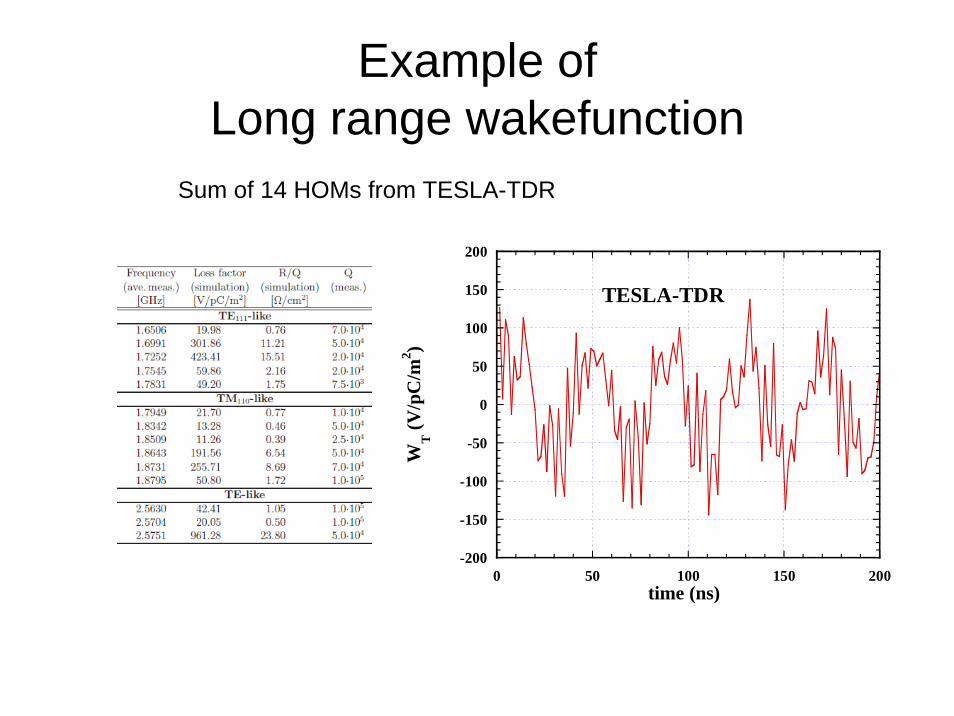
Example of Long range wakefunction
Sum of 14 HOMs from TESLA-TDR
-200
-150
-100
-50
0
50
100
150
200
0 50 100 150 200
TESLA-TDR
WT (V
/pC
/m2 )
time (ns)
Mitigation of long range transverse wakefield effect
• Damping– Extract higher order mode energy from
cavities through HOM couplers.• Detuning
– Cavity by cavity frequency spread.• Designed spread or• Random spread (due to errors)
• In LC, both will be necessary.
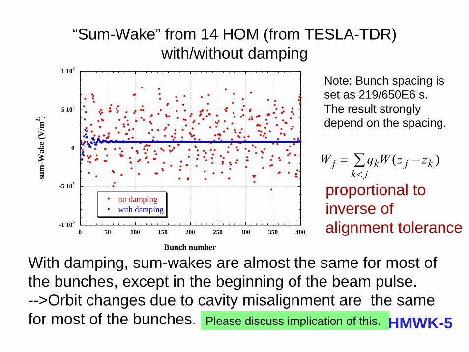
“Sum-Wake” from 14 HOM (from TESLA-TDR) with/without damping
Note: Bunch spacing is set as 219/650E6 s.The result strongly depend on the spacing.
)(∑<
−=jk
kjkj zzWqW
With damping, sum-wakes are almost the same for most of the bunches, except in the beginning of the beam pulse.-->Orbit changes due to cavity misalignment are the same for most of the bunches. Please discuss implication of this.
-1 106
-5 105
0
5 105
1 106
0 50 100 150 200 250 300 350 400
no dampingwith damping
sum
-Wak
e (V
/m2 )
Bunch number
HMWK-5
proportional to inverse of alignment tolerance
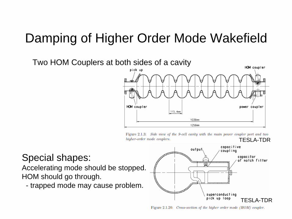
Damping of Higher Order Mode Wakefield
Two HOM Couplers at both sides of a cavity
TESLA-TDR
TESLA-TDR
Special shapes:Accelerating mode should be stopped.HOM should go through.- trapped mode may cause problem.

Detuning of wakefield
10 offactor by reduction Wakefield50bunch)next (next ns 500~for effectivefully becomes Detuning
MHz2~ 0.1% spread 2GHz,~frequency HOM Typical Linac,Main ILCIn
.2/ of Amplitude
,/2for , spread has If, of Amplitude
spread, no has If
sin
function,-betatocomparablelength in cavities
effective
effective
1effective
→≈→
→≈
≈
>≈
≈ ∑=
nt
WnW
tWnW
tWW
n
i
i
n
ii
ω
ωω
δ
δπδω
ω
ω
In X-band warm LC, carefully designed damped-detuned structures were necessary. Not for ILC.
ωi: HOM frequency of i-th cavity
For BBU: effective wake is from sum of cavities within length comparable to beta-function

Wakefunction envelope from HOMs (from TESLA-TDR) with/without random detuning (50 cavities) and damping
No detuning
Random detuningσf/f=0.1%
1
10
100
0 1 103 2 103 3 103 4 103 5 103 6 103
σf=0, no damp
σf=0, dampW
enve
lope
(V/p
C/m
2 )
time (ns)
1
10
100
0 1 103 2 103 3 103 4 103 5 103 6 103
fsf=0.1%, no damp
σf=0.1%, damp
Wen
velo
pe (V
/pC
/m2 )
time (ns)
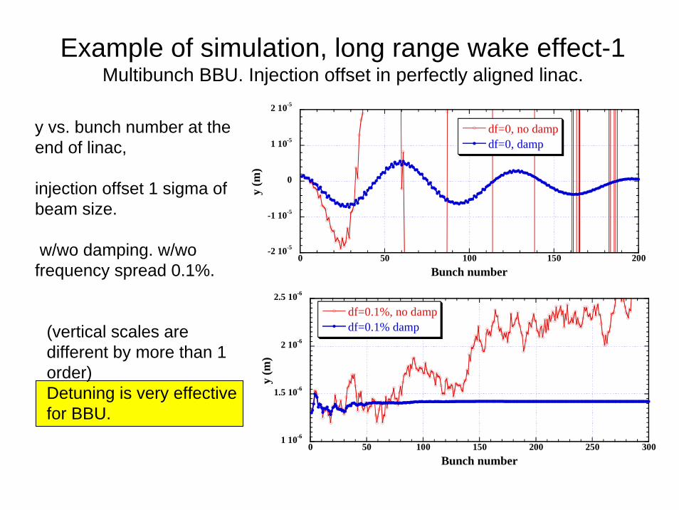
Example of simulation, long range wake effect-1Multibunch BBU. Injection offset in perfectly aligned linac.
y vs. bunch number at the end of linac,
injection offset 1 sigma of beam size.
w/wo damping. w/wo frequency spread 0.1%.
1 10-6
1.5 10-6
2 10-6
2.5 10-6
0 50 100 150 200 250 300
df=0.1%, no dampdf=0.1% damp
y (m
)
Bunch number
-2 10-5
-1 10-5
0
1 10-5
2 10-5
0 50 100 150 200
df=0, no dampdf=0, damp
y (m
)Bunch number
(vertical scales are different by more than 1 order)Detuning is very effective for BBU.

Example of simulation, long range wake effect-2Multibunch, random misalignment of cavities
y vs. bunch number at the end of linac,
Misalignment of cavities, sigma=0.5 mm..w/wo damping. w/wo frequency spread 0.1%.
-3 10-5
-2 10-5
-1 10-5
0
1 10-5
2 10-5
3 10-5
0 50 100 150 200
df=0, no dampdf=0, damp
y (m
)
Bunch number
-3 10-5
-2 10-5
-1 10-5
0
1 10-5
2 10-5
3 10-5
0 50 100 150 200 250 300
df=0.1%, no dampdf=0.1%, damp
(vertical scales are the same)Detuning is not so effective for random misalignment as for BBU.
• Horizontal beam orbit will be less stable than vertical. (Horizontal emittance is much larger than vertical, more than factor of 400 at the DR extraction.)
• Some dipole modes of wakefield may be x-y coupled
• Horizontal orbit may induce vertical orbit.
SKIPPossible vertical orbit induced by long range wakefield excited by horizontal orbit
x-y coupling of wakefield mode
Consider dipole wakefield.
If cavity is perfectly x-y symmetric, two polarization modes has the same frequency (perfectly degenerated.)Induced field by particles with horizontal offset kicks following particles only horizontally.
If symmetry is broken, two polarization have different frequencyand their axis can be slant.Induced field by particles with horizontal offset consists of two slant modes and can kick following particles vertically too.
SKIPx-y coupling of long range wakefield

θx
y
axis of mode-1
axis of mode-2
charge ttWxeq
tWtWtWtWtWtW
tWtWtWtW
eqWWWxeqW
y
x
ωθ
θθθθ
ωωθθ
cos)2/sin(2sin
cos)(sin)()(sin)(cos)()()2/sin()0()(
)2/sin()0()(sin)0(cos)0(
21
21
22
11
2
1
Δ−=
+=−=
Δ+=Δ−=
−==
-1.2
-0.8
-0.4
0
0.4
0.8
1.2
0 20 40 60 80 100 120
WxWy
W
t
SKIPx-y coupling of long range wakefield

• Extremely good cylindrical symmetry of cavities. Δ 0 : difficult? and/or cost?
• Stronger damping : difficult?• Intentionally broken symmetry. θ 0 : cost?• x-y tune difference (Different phase advance
per FODO cell). Suppress the effect of the coupling.
• etc. ???
SKIPCures of x-y coupling due to long range wakefield
Dispersive effect
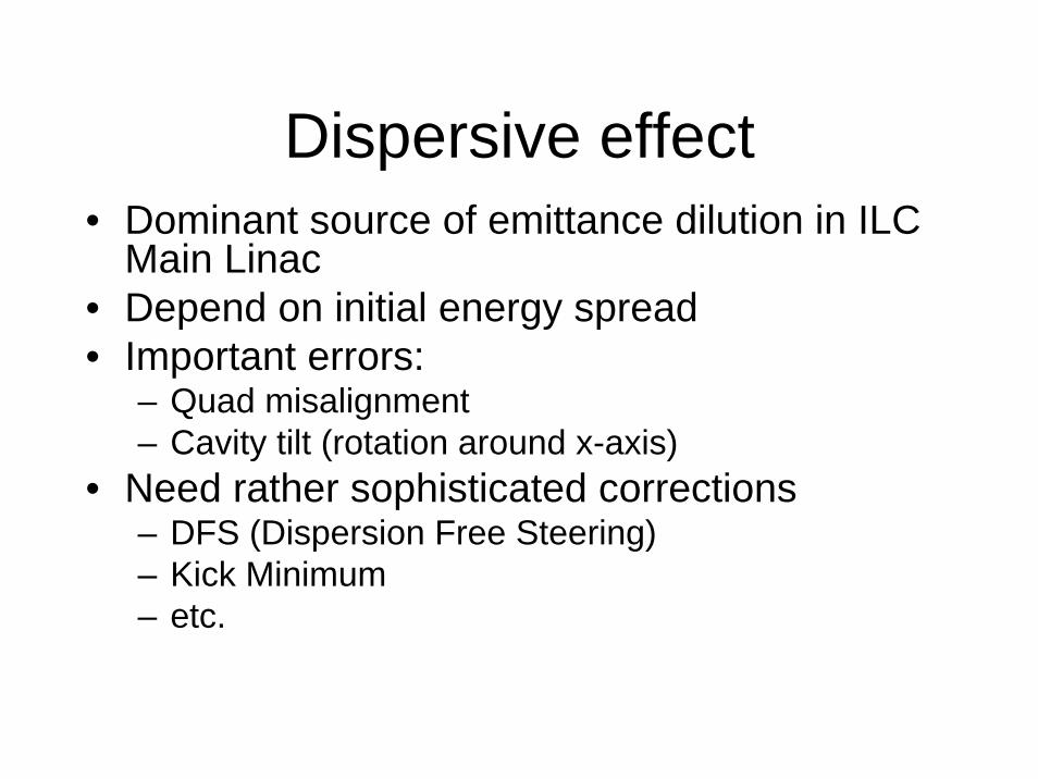
Dispersive effect• Dominant source of emittance dilution in ILC
Main Linac• Depend on initial energy spread• Important errors:
– Quad misalignment– Cavity tilt (rotation around x-axis)
• Need rather sophisticated corrections– DFS (Dispersion Free Steering)– Kick Minimum– etc.
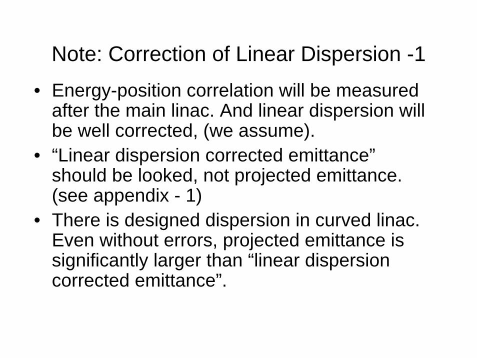
Note: Correction of Linear Dispersion -1
• Energy-position correlation will be measured after the main linac. And linear dispersion will be well corrected, (we assume).
• “Linear dispersion corrected emittance”should be looked, not projected emittance. (see appendix - 1)
• There is designed dispersion in curved linac. Even without errors, projected emittance is significantly larger than “linear dispersion corrected emittance”.

Note: Correction of Linear Dispersion -2• In principle, correction of non-linear dispersion is
possible. But practically, it will be very difficult. Only 1st order dispersion can be measured and corrected (practically).
• Even if 1st order dispersion is corrected at the end of linac, there can be large higher order dispersion remained.
• Transverse E-M fields at zero dispersion will induce linear (1st order) dispersion. And transverse, position dependent E-M fields (quad magnet) at non-zero n-th order dispersion will induce (n+1)th order dispersion.
• 1st order dispersion should be kept small everywhere in the linac to suppress higher order dispersions, then for preservation of low emittance.
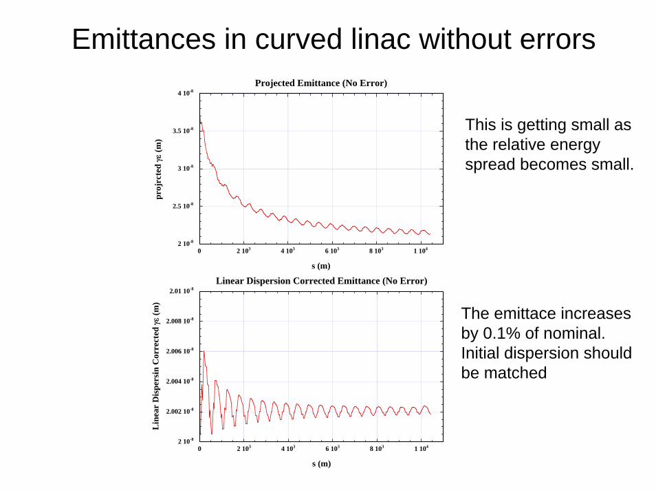
Emittances in curved linac without errors
2 10-8
2.5 10-8
3 10-8
3.5 10-8
4 10-8
0 2 103 4 103 6 103 8 103 1 104
Projected Emittance (No Error)
proj
rcte
d γε
(m)
s (m)
2 10-8
2.002 10-8
2.004 10-8
2.006 10-8
2.008 10-8
2.01 10-8
0 2 103 4 103 6 103 8 103 1 104
Linear Dispersion Corrected Emittance (No Error)
Lin
ear
Dis
pers
in C
orre
cted
γε (m
)
s (m)
The emittace increases by 0.1% of nominal.Initial dispersion should be matched
This is getting small as the relative energy spread becomes small.
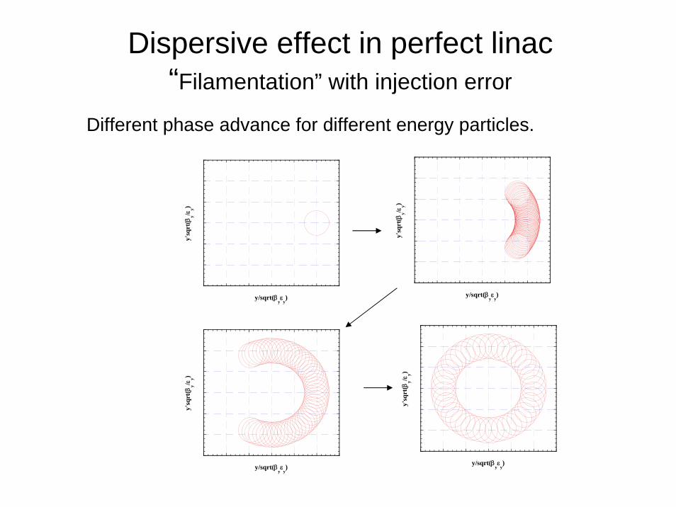
Dispersive effect in perfect linac “Filamentation” with injection error
y'sq
rt(β
y/εy)
y/sqrt(βyε
y)
y'sq
rt(β
y/εy)
y/sqrt(βyε
y)
y'sq
rt(β
y/εy)
y/sqrt(βyε
y)
y'sq
rt(β
y/εy)
y/sqrt(βyε
y)
Different phase advance for different energy particles.
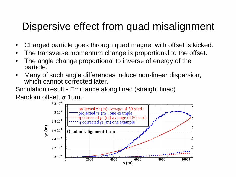
Dispersive effect from quad misalignment• Charged particle goes through quad magnet with offset is kicked.• The transverse momentum change is proportional to the offset.• The angle change proportional to inverse of energy of the
particle.• Many of such angle differences induce non-linear dispersion,
which cannot corrected later.Simulation result - Emittance along linac (straight linac)Random offset, σ 1um..
2 10-8
2.2 10-8
2.4 10-8
2.6 10-8
2.8 10-8
3 10-8
3.2 10-8
0 2000 4000 6000 8000 10000
projected γε (m) average of 50 seedsprojected γε (m), one exampleη corrected γε (m) average of 50 seedsη corrected γε (m) one example
γε (m
)
s (m)
Quad misalignment 1 μm
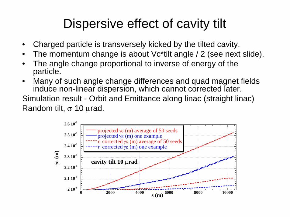
Dispersive effect of cavity tilt• Charged particle is transversely kicked by the tilted cavity.• The momentum change is about Vc*tilt angle / 2 (see next slide).• The angle change proportional to inverse of energy of the
particle. • Many of such angle change differences and quad magnet fields
induce non-linear dispersion, which cannot corrected later.Simulation result - Orbit and Emittance along linac (straight linac)Random tilt, σ 10 μrad.
2 10-8
2.1 10-8
2.2 10-8
2.3 10-8
2.4 10-8
2.5 10-8
2.6 10-8
0 2000 4000 6000 8000 10000
cavity tilt 10 μrad
projected γε (m) average of 50 seedsprojected γε (m) one exampleη corrected γε (m) average of 50 seedsη corrected γε (m) one example
γε (m
)
s (m)

beam
Transverse kick in the cavity: Δpt = θ eEL
offset: y0+Lθ/2 offset: y0-Lθ/2
entrance exitEdge (de)focus [see appendix]
Transverse kick at the entrance: Δpt = -eE (y0+θ L/2)/2Transverse kick at the exit: Δpt = eE (y0-θ L/2)/2
Total transverse kick by the cavity: Δpt = θ eEL/2
SKIPNote: Edge focus reduce the effect of cavity tiltAcc. field E, length L, tilt angle θ

Static corrections(transverse motion)
Necessity of Beam based corrections
• Without corrections, required alignment accuracy to keep emittance small will be, roughly:– 0.1~1 um for quad offset– 1~10 urad for cavity tiltwhich will not be achieved.(cavity offset ~ a few 100 um may not be
serious problem.)
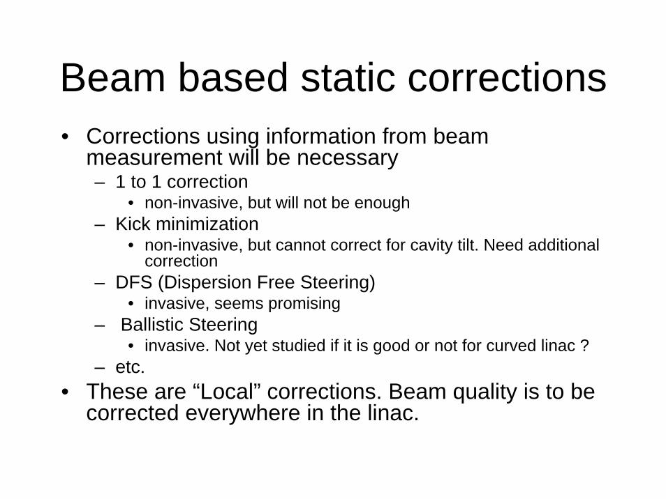
Beam based static corrections• Corrections using information from beam
measurement will be necessary– 1 to 1 correction
• non-invasive, but will not be enough– Kick minimization
• non-invasive, but cannot correct for cavity tilt. Need additional correction
– DFS (Dispersion Free Steering) • invasive, seems promising
– Ballistic Steering• invasive. Not yet studied if it is good or not for curved linac ?
– etc. • These are “Local” corrections. Beam quality is to be
corrected everywhere in the linac.
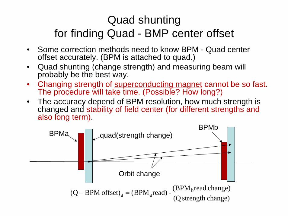
Quad shunting for finding Quad - BMP center offset
• Some correction methods need to know BPM - Quad center offset accurately. (BPM is attached to quad.)
• Quad shunting (change strength) and measuring beam will probably be the best way.
• Changing strength of superconducting magnet cannot be so fast. The procedure will take time. (Possible? How long?)
• The accuracy depend of BPM resolution, how much strength is changed and stability of field center (for different strengths and also long term).
BPMaBPMb
quad(strength change)
Orbit change
change)strength (Qchange)readBPM(-read)BPM(offset) BPM(Q b
aa =−
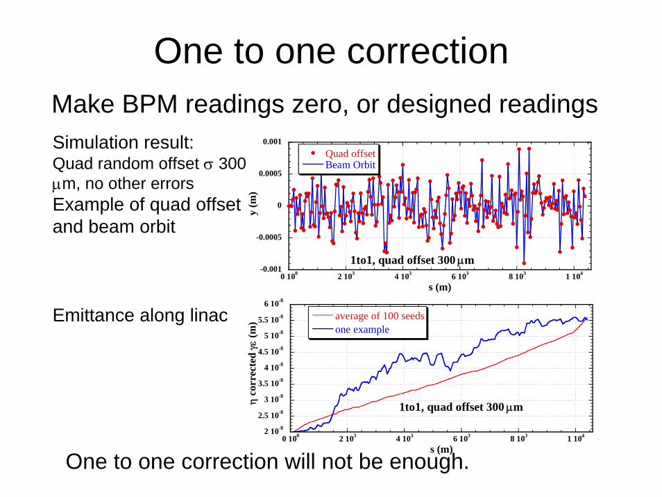
One to one correctionMake BPM readings zero, or designed readings
2 10-8
2.5 10-8
3 10-8
3.5 10-8
4 10-8
4.5 10-8
5 10-8
5.5 10-8
6 10-8
0 100 2 103 4 103 6 103 8 103 1 104
1to1, quad offset 300 μm
average of 100 seedsone example
η co
rrec
ted
γε (m
)
s (m)
-0.001
-0.0005
0
0.0005
0.001
0 100 2 103 4 103 6 103 8 103 1 104
1to1, quad offset 300 μm
Quad offsetBeam Orbit
y (m
)
s (m)
Simulation result:Quad random offset σ 300 μm, no other errorsExample of quad offset and beam orbit
Emittance along linac
One to one correction will not be enough.
• Basically:– Steer beam to minimize kick angle at every quadrupole-
dipole magnet pair. Or minimize deviation from designed kick angle. (Requiring Quad and dipole magnets are attached or very close each other.)
– See appendix for a little more details• Can be non-invasive correction
– may be used as a “dynamic correction” for relatively slow quad motions.
• Accurate information of Quad - BPM offset is important.
• Can correct quad misalignment but not effective for cavity tilt.
SKIPKick Minimization (KM)
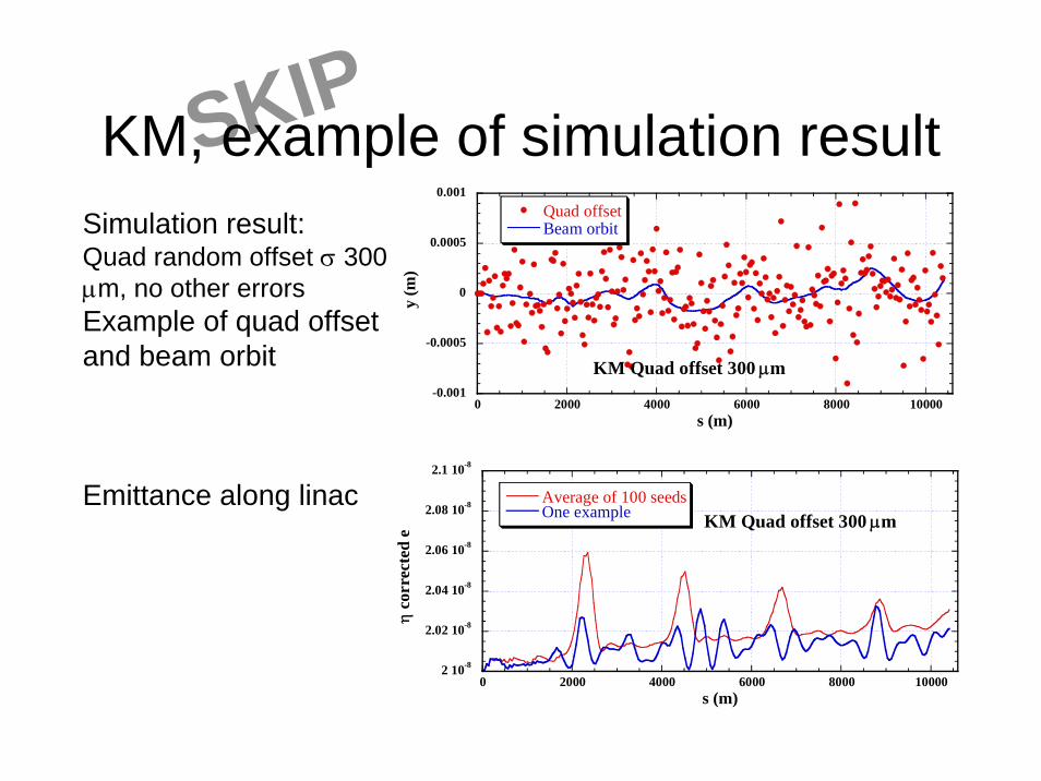
Simulation result:Quad random offset σ 300 μm, no other errorsExample of quad offset and beam orbit
Emittance along linac
-0.001
-0.0005
0
0.0005
0.001
0 2000 4000 6000 8000 10000
KM Quad offset 300 μm
Quad offsetBeam orbit
y (m
)s (m)
2 10-8
2.02 10-8
2.04 10-8
2.06 10-8
2.08 10-8
2.1 10-8
0 2000 4000 6000 8000 10000
KM Quad offset 300 μmAverage of 100 seedsOne example
η co
rrec
ted
e
s (m)
SKIPKM, example of simulation result
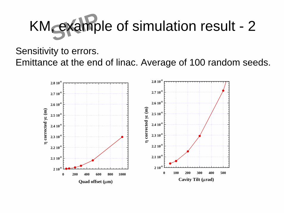
Sensitivity to errors.Emittance at the end of linac. Average of 100 random seeds.
2 10-8
2.1 10-8
2.2 10-8
2.3 10-8
2.4 10-8
2.5 10-8
2.6 10-8
2.7 10-8
2.8 10-8
0 200 400 600 800 1000
η c
orre
cted
γε
(m)
Quad offset (μm)
2 10-8
2.1 10-8
2.2 10-8
2.3 10-8
2.4 10-8
2.5 10-8
2.6 10-8
2.7 10-8
2.8 10-8
0 100 200 300 400 500
η c
orre
cted
γε
(m)
Cavity Tilt (μrad)
SKIPKM, example of simulation result - 2

DFS (Dispersion Free Steering)• Basically:
– Change beam energy and measure beam orbit. – Steer beam to minimize orbit difference. Or, minimize
deviation from designed orbit difference in the case of the curved linac.
– See appendix for an example of algorithms (not necessarily the best one)
• Results seem to depend on some details of algorithms. (?)
• Need to change accelerating voltage to change beam energy. ~ 10%– How accurately it can be, practically???
• BPM resolution is important but information of Quad -BPM offset is not so important.– Because “difference of orbit” is looked at.
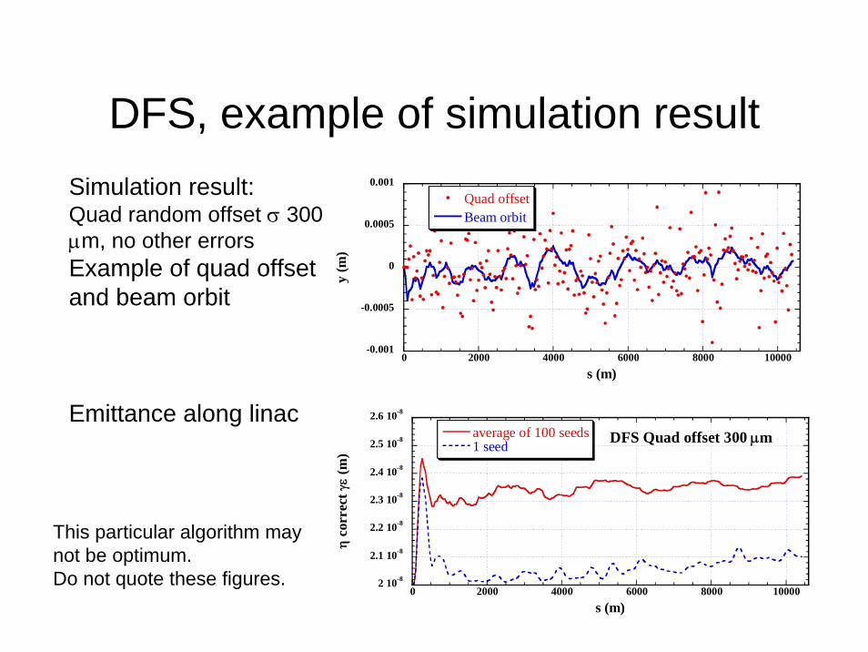
DFS, example of simulation resultSimulation result:Quad random offset σ 300 μm, no other errorsExample of quad offset and beam orbit
Emittance along linac
This particular algorithm may not be optimum.Do not quote these figures.
-0.001
-0.0005
0
0.0005
0.001
0 2000 4000 6000 8000 10000
Quad offsetBeam orbit
y (m
)
s (m)
2 10-8
2.1 10-8
2.2 10-8
2.3 10-8
2.4 10-8
2.5 10-8
2.6 10-8
0 2000 4000 6000 8000 10000
DFS Quad offset 300 μmaverage of 100 seeds1 seed
η c
orre
ct γ
ε (m
)
s (m)
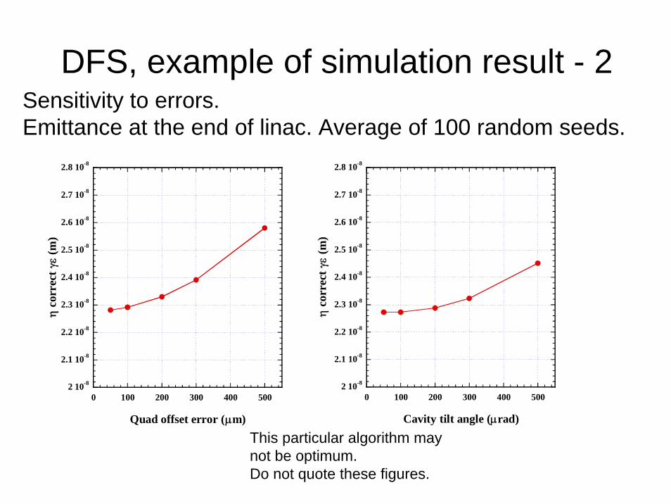
DFS, example of simulation result - 2Sensitivity to errors.Emittance at the end of linac. Average of 100 random seeds.
This particular algorithm may not be optimum.Do not quote these figures.
2 10-8
2.1 10-8
2.2 10-8
2.3 10-8
2.4 10-8
2.5 10-8
2.6 10-8
2.7 10-8
2.8 10-8
0 100 200 300 400 500
η c
orre
ct γ
ε (m
)
Quad offset error (μm)
2 10-8
2.1 10-8
2.2 10-8
2.3 10-8
2.4 10-8
2.5 10-8
2.6 10-8
2.7 10-8
2.8 10-8
0 100 200 300 400 500
η co
rrec
t γε
(m)
Cavity tilt angle (μrad)
“Global” corrections
• In addition to “Local” corrections.• Scan knobs, measuring beam at the end of
the linac or certain linac section, and finding the best setting of the knobs.
• For ILC, we are considering:– Knobs: Orbit bumps– Measurement: emittance or beam size– Correct dispersive effect: “Dispersion bumps”– Correct wakefield effect: “Wakefield bumps”

Dispersion Bumps and Wakefield Bumps• Energy-dependent kick (dispersion) or/and z-
dependent kick (wakefield) in the section is to be compensated by the bumps.– Possible (in principle) by two bumps, phase
advance 90 deg. apart. – The length of the section should not be so long.
Induced dispersion or z-x/y correlation (by wakefield) should be corrected before significant filamentation.
bump -> tail is kicked Monitortail is kicked by errorCancelled
phase advance ~90o bumps may be just before the monitor

Dynamic corrections (Feedback)

Dynamic errors• Mechanical motion
– Motion induced by the machine itself (motors for cooling, bobbles in pipes, etc.)
– Cultural noise (nearby traffic, etc.)– Ground motion (slow movement, earth quake)
• Strength– Field strength of magnets– Accelerating field, amplitude and phase
• EM field from outside– no problem for high energy beam (?)

Typical speed of fluctuations and correctionsfor transverse motion
Speed (Hz) Possible source Effective correction For
>106 DR kickers, what else ?Machine, cultural noise, Power supply, ground motion
Feed forward (in turnaround)
Temperature change, ground motion,
What else?
1 ~ 106 Intra pulse feedback at IP
Position
Position
Position
Emittance
0.001 ~ 1 Simple orbit feedback (in BDS and Linac)
? ~ 0.01 More sophisticated orbit FB(, e.g. KM, If necessary).
0 ~ 0.0001? Emittance“static” corrections

Note on Dynamic correction in ILC Main Linac - 1
Some simulations studies were, (and are being), performed. But,
Studies have not well matured for ILC and there is no commonly agreed scheme, but probably:
1. Orbit correction at several locations.2. Energy feed back. One or two locations / linac (?)3. One-to-one orbit correction (using all or most correctors
and BPM, slower than1) 4. Some non-invasive corrections, if necessary.
Need to be careful from Machine protection point of view.IF feedbacks change machine parameter too much, the beam may
hit some part of machine.
Note on Dynamic correction in ILC Main Linac - 2
Dynamic errors (component position movement, field strength fluctuations) during “static”tuning can be problem.
• “Static” tuning will take time (many minutes or an hour or ?)
• “Static” tuning assumes (requires) stability of the machine during beam measurements and corrections.
This effect is not expected to be so serious (?), but has not been well studied.
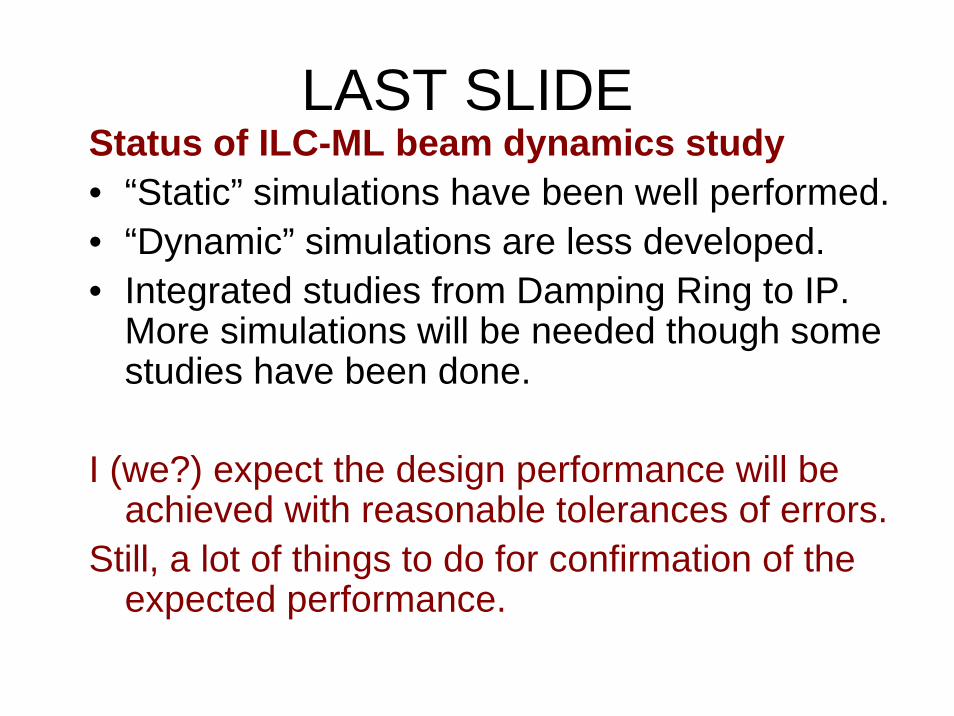
LAST SLIDEStatus of ILC-ML beam dynamics study• “Static” simulations have been well performed.• “Dynamic” simulations are less developed.• Integrated studies from Damping Ring to IP.
More simulations will be needed though some studies have been done.
I (we?) expect the design performance will be achieved with reasonable tolerances of errors.
Still, a lot of things to do for confirmation of the expected performance.

Appendix - 1
Definition ofProjected emittance andLinear Dispersion Corrected emittance
Projected emittance
≡ (< y2 > − < y >2 )(< y'2 > − < y'>2 ) − (< yy'> − < y >< y'>)2
y : Vertical offset, y': Verticale angleδ : Relative energy deviation
η ≡ (< yδ > − < y >< δ >) /(< δ2 > − < δ >2), η'≡ (< y'δ > − < y'>< δ >) /(< δ2 > − < δ >2 )< >: Average over all macro - particles
Linear Dispersion Corrected emittance
≡ (< (y − ηδ)2 > − < y − ηδ >2)(< (y'−η'δ)2 > − < y'−η'δ >2 ) − (< (y − ηδ)(y'−η'δ) > − < y − ηδ >< y'−η'δ >)2
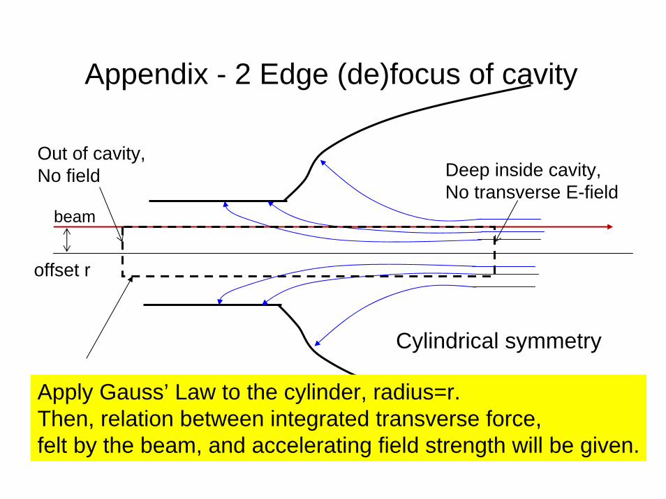
Appendix - 2 Edge (de)focus of cavity
beam
Deep inside cavity,No transverse E-field
offset r
Out of cavity,No field
Apply Gauss’ Law to the cylinder, radius=r.Then, relation between integrated transverse force,felt by the beam, and accelerating field strength will be given.
Cylindrical symmetry
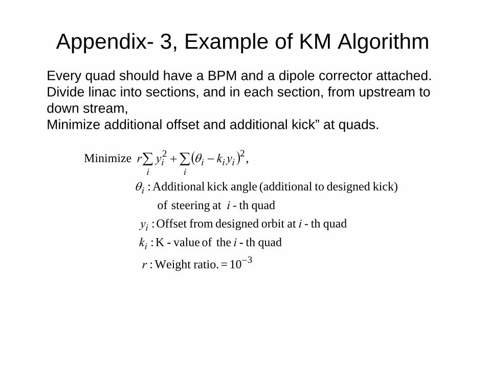
Appendix- 3, Example of KM AlgorithmEvery quad should have a BPM and a dipole corrector attached. Divide linac into sections, and in each section, from upstream to down stream,Minimize additional offset and additional kick” at quads.
( )
3
22
10= ratio. Weight :
quadth - theof value-K : quadth -at orbit designed fromOffset :
quadth -at steering of kick) designed tol(additiona anglekick Additional :
, Minimize
−
∑∑ −+
r
ikiy
i
ykyr
i
i
i
iiii
ii
θ
θ
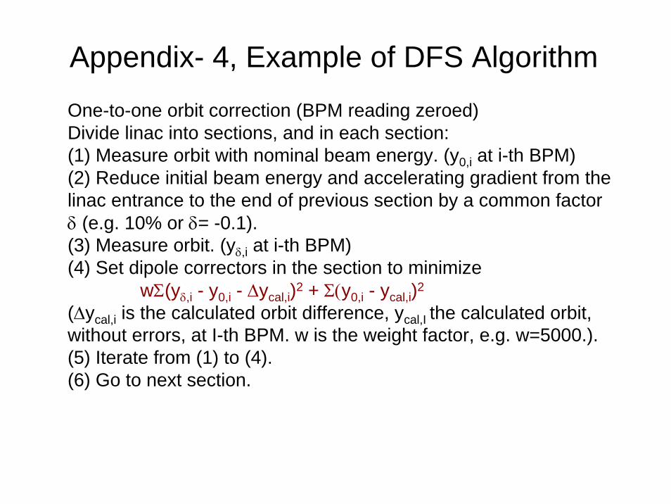
Appendix- 4, Example of DFS AlgorithmOne-to-one orbit correction (BPM reading zeroed)Divide linac into sections, and in each section:(1) Measure orbit with nominal beam energy. (y0,i at i-th BPM)(2) Reduce initial beam energy and accelerating gradient from the linac entrance to the end of previous section by a common factorδ (e.g. 10% or δ= -0.1).(3) Measure orbit. (yδ,i at i-th BPM)(4) Set dipole correctors in the section to minimize
wΣ(yδ,i - y0,i - Δycal,i)2 + Σ(y0,i - ycal,i)2
(Δycal,i is the calculated orbit difference, ycal,I the calculated orbit,without errors, at I-th BPM. w is the weight factor, e.g. w=5000.).(5) Iterate from (1) to (4).(6) Go to next section.