Contents lists available at ScienceDirect

Developmental Cognitive Neuroscience

journal homepage: www.elsevier.com/locate/dcn

Making an unknown unknown a known unknown: Missing data inlongitudinal neuroimaging studies

Tyler H. Mattaa,⁎, John C. Flournoyb, Michelle L. Byrneb

a Centre for Educational Measurement at the University of Oslo, NorwaybDepartment of Psychology, University of Oregon, Eugene, OR, USA

A R T I C L E I N F O

Keywords:NeuroimagingMissing dataLikelihoodLongitudinal data

A B S T R A C T

The analysis of longitudinal neuroimaging data within the massively univariate framework provides the op-portunity to study empirical questions about neurodevelopment. Missing outcome data are an all-to-commonfeature of any longitudinal study, a feature that, if handled improperly, can reduce statistical power and lead tobiased parameter estimates. The goal of this paper is to provide conceptual clarity of the issues and non-issuesthat arise from analyzing incomplete data in longitudinal studies with particular focus on neuroimaging data.This paper begins with a review of the hierarchy of missing data mechanisms and their relationship to likelihood-based methods, a review that is necessary not just for likelihood-based methods, but also for multiple-imputationmethods. Next, the paper provides a series of simulation studies with designs common in longitudinal neuroi-maging studies to help illustrate missing data concepts regardless of interpretation. Finally, two applied ex-amples are used to demonstrate the sensitivity of inferences under different missing data assumptions and howthis may change the substantive interpretation. The paper concludes with a set of guidelines for analyzingincomplete longitudinal data that can improve the validity of research findings in developmental neuroimagingresearch.

1. Introduction

A number of neuroimaging techniques, including structural andfunctional magnetic resonance imaging (s/fMRI), have been employedto collect data that enable researchers to study the relation betweenneurobiology, cognition, and behavior. These techniques result inthousands of voxels per experimental unit, or participant, and are ty-pically analyzed in a massively univariate framework, that is, by fittingthe same statistical model to each voxel (Friston et al., 1995). Morerecently, neuroimaging data has been collected under repeated mea-sures study designs, providing researchers with the opportunity to studyempirical questions about neurodevelopment. The analysis of long-itudinal neuroimaging data remains within the massively univariateframework where a growth model is fit to the repeated measures ofeach voxel. Thus, while the analysis of longitudinal neuroimaging datais relatively new, the field has the opportunity to exploit decades ofmethodological developments in longitudinal data analysis. One ad-vantage of a longitudinal study designs over cross-sectional designs isthat by collecting measures from study participants over multiple oc-casions, or waves, the analyst can test theories about development that

do not conflate cohort effects with temporal effects (Skrondal and Rabe-Hesketh, 2004; Diggle et al., 2002). An all-to-common feature oflongitudinal studies, regardless of the substantive area, is that somemeasures for some participants will go uncollected. That is, some par-ticipants may miss one or more waves of data collection intermittentlythroughout the study while others may dropout of the study altogether.How to obtain valid inferences for key model parameters in the pre-sence of missing data has been a major focus in statistics for more than40 years. The statistical literature uses the term incomplete data inter-changeably with missing data in the context of longitudinal studies. Thepioneering work of Rubin (1976) and Little (1976) introduced the is-sues associated with analyzing incomplete data and their impact onparameter estimates. More than forty years later, the analysis of in-complete data has grown into a prolific, currently active literature instatistics (e.g.,Mealli and Rubin, 2015; Seaman et al., 2013). Whenpresented with missing data, the researcher must make assumptionsabout the reason(s) why the data went uncollected and realize thatvalid inferences rest on how those assumptions are operationalized.However, as we will make clear later in this paper, the nature of themissing data depends on the data that went uncollected, leaving the

https://doi.org/10.1016/j.dcn.2017.10.001Received 15 March 2017; Received in revised form 3 September 2017; Accepted 6 October 2017

⁎ Corresponding author at: Postboks 1161, Blindern 0318, Oslo, Norway.E-mail address: tyler.matta@cemo.uio.no (T.H. Matta).

Abbreviation: MAR, missing at random; MAAR, missing always at random; MCAR, missing completely at random; MACAR, missing always completely at random; MNAR, missing not atrandom; MNAAR, missing not always at random

Developmental Cognitive Neuroscience xxx (xxxx) xxx–xxx

1878-9293/ © 2017 The Authors. Published by Elsevier Ltd. This is an open access article under the CC BY-NC-ND license (http://creativecommons.org/licenses/BY-NC-ND/4.0/).

Please cite this article as: Matta, T.H., Developmental Cognitive Neuroscience (2017), http://dx.doi.org/10.1016/j.dcn.2017.10.001

researcher unable to explicitly test the validity of those assumptions. Asa result, there is no empirical way to determine which missing dataassumption is correct (Molenberghs et al., 2008), making the assess-ment of multiple assumptions, often referred to as sensitivity analysis,even more critical. While attention to missing data and an awareness ofappropriate methods analyzing incomplete data are critical for validinferences, its import may not be fully understood across the develop-mental psychology field. Jelicić et al. (2009) conducted a systematicreview of studies with developmental samples and showed that 82%used methods that place overly strict assumptions about the missingdata. For example, many of those studies chose to omit subjects withmissing data completely (i.e., list-wise deletion or complete case ana-lysis), which may result in unacceptable levels of bias when general-izing to the intended population and reduces statistical power. Thesedeletion methods also negate the effort from both researchers and studyparticipants in collecting the available data. Indeed, opting to discardcollected data when best practice indicates their use would very likelycontravene our obligations under ethical guidelines for the use ofhuman subjects. Misunderstanding and/or ignorance of the statisticalissues associated with analyzing missing data could also contribute todiscrepancies observed between datasets acquired across different la-boratories and prevent replication efforts— a problem that has recentlyreceived noticeable attention and concern in the fields of neuroscienceand psychology more broadly (Gorgolewski and Poldrack, 2016). Initialintuition often suggests it is better to remove those study participantswho have missing data because there is no way of knowing what themissing values could have been. To many researchers, the treatment ofmissing data is seen as “making up” data, akin to waving a magic wand.And we agree that missing data is a theoretically challenging aspect ofapplied data analysis. With that, given that the analysis of longitudinalneuroimaging data is relatively new, we believe that it is much moredifficult to reverse misconceptions than it is to properly introduceconcepts from the beginning. Therefore, rather than rush through thestatistical aspects of missing data and simply provide a list of tools thata researcher might employ when presented with missing data, the goalof this paper is to provide conceptual clarity of the issues (and non-issues) that arise from analyzing incomplete data in longitudinal stu-dies. Although there are three general methods for analyzing in-complete data undergoing active development, (a) likelihood-based(including Bayesian), (b) multiple imputation, and (c) weighting, wefocus on likelihood-based methods because (a) we believe it illustratesthe issues of analyzing incomplete data clearly and (b) it is embodied inmultiple imputation techniques. At the end of the paper, we offer fur-ther explanation for our choice of focusing on likelihood-basedmethods. Furthermore, we limit the paper to issues with missing out-come data (e.g., missing f/sMRI scans). To achieve this goal, the paperproceeds as follows. In Section 2, we review key contributions in thestatistical literature on the relationship between likelihood-based in-ference and missing data. While notationally intensive and general, thissection is required to foster an understanding of the statistical under-pinnings that enable us to obtain valid inferences in the presence ofincomplete data. We do not assume the reader is already familiar withthis notation and devote space to translating much of the notation intoplain English. In Section 3, we provide a set of simple simulations in aneffort illustrate the statistical concepts covered in the previous section,focusing on how estimates change as a function of the missing datamechanism and how the data are analyzed. For Section 4, we re-analyzetwo longitudinal neuroimaging datasets, one fMRI and one sMRI, todemonstrate the sensitivity of inferences under different missing dataassumptions and how this may change the substantive interpretation.Finally, in Section 5, we provide a discussion of the results and presentthree guidelines for analyzing incomplete longitudinal neuroimagingdata.

2. Missing data

In order to review the concepts of missing data, particularly as theyrelate to longitudinal studies, some notation must be introduced.Recent literature (e.g., Mealli and Rubin, 2015; Seaman et al., 2013)has observed that the notation used to express concepts about missingdata has shifted from that which was introduced by Rubin (1976) intosomething less precise, possibly creating confusion for readers. Giventhis, we do our best to adhere the notation of Rubin (1976) and Mealliand Rubin (2015) to review key concepts of analyzing longitudinal datawith dropout. For simplicity, we consider the balanced repeated mea-sures study. For participant i= 1, 2, …, N, there is an intent to collectj = 1, 2, …, n repeated measurements of the response variable of in-terest. Thus, let Yi be a vector for participant i's n longitudinal out-comes, and = ′ ′ … ′ ′Y Y Y Y( , , , )N1 2 be a vector for n · N observations of alloutcomes in the sample.1 Let us assume (again for simplicity) that eachobservation Yij in Yi is a continuous unknown real number that can takea value from the range of possible values (as defined by the samplingand measurement instrument) known as the sample space Ω. Finally, letXi be an n × p matrix containing fixed covariates and the variable orvariables that define how observations relate to the passage of time,where p is the number of covariates and time-defining variables. Thegoal of such a hypothetical study is to obtain correct inferences for thevector of unknown parameters θ that govern the conditional multi-variate density fY(Y|X, θ) — that is, we estimate θ in order to learnsomething about how time, and our covariates in X relate to the out-come Y. Although the study intends to collect n repeated measures fromthe N participants, there will be those participants in the study who failto provide all n responses. Therefore, let Ri be participant i's length nvector of observed-data indicators where Rij = 1 if Yij is observed (i.e.,taking a valid value in the sampling space Ω) and Rij = 0 if Yij is missing(and so has the potential to take any value in Ω). The vector

= ′ ′ … ′ ′R R R R( , , , )N1 2 is the pattern of observed and missing measure-ments for each participant at each measurement occasion. Given thevector of observed-data indicators Ri, the vector Yi can be partitionedinto two ordered subvectors: those responses that are observed andthose responses that are missing, denoted as Yi,(1) and Yi,(0), respec-tively. This partitioning enables us to be explicit about our handling ofthe observed outcomes and the unobserved outcomes. The missing datamechanism is the statistical model for the observed-data indicators,fR(R|Y, X, Z, α). That is, missing data, R, may depend on the outcome ofinterest Y, the covariates of interest X, as well as a distinct set of cov-ariates not related to Y, indicated by Z. Additionally α is the set ofparameters that govern this relation, a set of parameters that are dis-tinct from the parameters that govern the relation between Y and X(that is, θ). In the broad context of a statistical analysis, this means wenow have a probability statement governing the outcome of interest Yas well as a probability statement governing the pattern of missing dataindicators, R. Still following the notation of Rubin (1976), let ri be ageneric value of Ri and ri be a particular sample realization of Ri.Likewise, let yi,(1) be a generic value for Yi,(1) and ∼yi,(1) be a samplerealization of Yi,(1). Clearly, there is no sample realization of Yi,(0) as itcontains the data that went unobserved for this particular sample so weonly speak of the generic version, yi,(0). Whether or not we can obtaincorrect inferences for θ using only Yi,(1), that is, ignoring Ri, dependsupon the nature of the missing data mechanism. The remainder of thissection provides an overview of the hierarchy of missing data me-chanisms and their association with likelihood-based methods.

1 You can also consider Y★ as an N × nmatrix where the outcomes for each participantoccupies a row.

T.H. Matta et al. Developmental Cognitive Neuroscience xxx (xxxx) xxx–xxx

2

2.1. Missing data hierarchy

2.1.1. Missing completely at randomOne can think of missing responses that are missing completely at

random, or MCAR, to be a random sample of the outcome vector Yi, orequivalently, those who complete the study without any missing dataare a random sample of the complete data vector. Stated more techni-cally, missing data are MCAR when the probability that responses aremissing, =R ri i, is independent of the observed responses obtained,

= ∼Y yi i,(1) ,(1), the responses that were intended to be obtained but werenot, Yi,(0) = yi,(0), and the set of covariates, Xi. In other words, missingdata are MCAR when Ri is independent of Y(1), Y(0), and Xi, statedprobabilistically as:

= = = = =∼ α αR r Y y Y y X Z R r Zℙ( | , , , , ) ℙ( | , ). i i i i i i i i i i i,(1) ,(1) ,(0) ,(0)

(1)

Note that Eq. (1) is a statement about the realized missing data, notabout the missing data mechanism itself. Mealli and Rubin (2015) in-troduced the term missing always completely at random, or MACAR,which provides specific language for a missing data mechanism thatwill always produce missing data that are missing completely atrandom.

= = = = =α αR r Y y Y y X Z R r Zℙ( | , , , , ) ℙ( | , ).i i i i i i i i i i i,(1) ,(1) ,(0) ,(0)

(2)

Notice that ri and ∼yi,(1) in Eq. (1) are replaced by ri and yi,(1) in Eq. (2) tosignify that any realization of Ri will be missing completely at random.Thus, Eq. (1) defines data that are MCAR and Eq. (2) defines theMACAR missing data mechanism.

2.1.1.1. Covariate-dependent missingness. Little (1995) distinguishedbetween MCAR as stated above and missingness that is conditionallyindependent of Yi given some set of covariates Xi, which he referred toas covariate-dependent missingness. Covariate-dependent missingness canbe stated probabilistically as

= = = = =∼ α αR r Y y Y y X Z R r X Zℙ( | , , , , ) ℙ( | , , ). i i i i i i i i i i i i,(1) ,(1) ,(0) ,(0)

(3)

This is to say, if data are missing because of a covariate associated withY, if that covariate is included in the model for Yi, then the parameterestimates based on Yi,(1) will be unbiased. It is important to note thatthe subset of covariates that Ri depends on must be included in themodel for Yi. If those covariates are not included in the model then Yi

remains dependent on Ri. Equally important to consider is that themodel fit without the covariate (or covariates) would also suffer fromomitted variable bias.

2.1.2. Missing at randomCompared to MCAR, the assumption of missing at random, or MAR, is

a less restrictive assumption in that the missing data can depend onYi,(1). Given the realized available data, = ∼Y yi i,(1) ,(1) and Xi, the prob-ability of obtaining the missing data =R ri i does not vary with possiblevalues of yi,(0) or with possible values of the parameter vector α (Rubin,1976; Mealli and Rubin, 2015). The MAR assumption may be statedprobabilistically as

= = = =

= = = ′

∼

∼

αα

R r Y y Y y X ZR r Y y Y y X Z

ℙ( | , , , , )ℙ( | , , , , )

i i i i i i i i

i i i i i i i i

,(1) ,(1) ,(0) ,(0)

,(1) ,(1) ,(0) ,(0) (4)

for all α, yi,(0) and ′y i,(0) . This equality says that the realized missing datamay depend on the set of observed responses Yi,(1) and covariates Xi,but is free of dependence on the unobserved responses Yi,(0). Themissing data mechanism is missing always at random, or MAAR, if wereplace =R ri i in Eq. (4) with Ri = ri and = ∼Y yi i,(1) ,(1) with Yi,(1) = yi,(1)(Mealli and Rubin, 2015).

2.1.3. Missing not at randomFinally, when missing data depend on the data that went un-

collected, Yi,(0), the data are said to be missing not at random, or MNAR.Data that are missing not at random can be defined probabilistically ifwe replace the equality in Eq. (4) with an inequality,

= = = ≠

= = = ′

∼

∼

αα

R r Y y Y y X ZR r Y y Y y X Z

ℙ( | , , , , )ℙ( | , , , , )

i i i i i i i i

i i i i i i i i

,(1) ,(1) ,(0) ,(0)

,(1) ,(1) ,(0) ,(0) (5)

for some α, and some ≠ ′y yi i,(0) ,(0) . Like the definitions above, sub-stituting =R ri i in Eq. (5) for Ri = ri and = ∼Y yi i with Yi = yi defines themissing not always at random mechanism, or MNAAR (Mealli and Rubin,2015).

2.2. Likelihood-based inference

Remaining in the context of longitudinal studies, recall that we seekto obtain correct inferences for the vector of unknown parameters θthat govern the conditional multivariate density fY(Y|X, θ). This is oftendone by finding the values of θ with the maximum likelihood Lθ(θ|y, X)or its logarithm, ℓθ(θ|y, X). When missing data are present, however,∼y(1) may not provide sufficient information about Y to obtain valid es-timates of θ. Thus, we would be naive to only consider ∼y without alsoconsidering r, which may provide necessary information about Y. Thatis, when presented with incomplete data, we must consider the jointdistribution of the available data, ∼y(1), and the missing data indicators,r, ∼ θ αf y r X Z( , | , , , )Y R, (1) and the log-likelihood ∼θ α y r Xℓ ( , | , , )θ α, (1)(Rubin, 1976; Kenward and Molenberghs, 1998) — in other words, itmay be the case that valid estimates of θ can only be obtained by es-timating θ and α jointly. How we specify the likelihood, using ℓθ or ℓθ,αdepends on our assumptions about the missing data mechanism. Rubin(1976) showed that when the missing data are MAR (with MCAR as aspecial case), the missing data mechanism is non-informative or ignor-able. When missing data are MNAR, however, the missing data me-chanism is informative or nonignorable.

2.2.1. Ignorable mechanisms2.2.1.1. Missing completely at random. When missing data is assumed tobe the result of an MACAR mechanism, the missing data indicator is(conditionally) independent of the responses. Thus, the jointdistribution of the observed data can be factorized as

=∼ ∼θ α θ αf f fy r X Z y X r X Z( , | , , , ) ( | , ) ( | , , ) Y R Y R, (1) (1) (6)

with log-likelihood

= +∼ ∼θ α θ αy r X Z y X r X Zℓ ( , | , , , ) ℓ ( | , ) ℓ ( | , , ). θ α θ α, (1) (1) (7)

Thus, when interest is in values of θ and α is merely a vector of nuisanceparameters, we can obtain valid inferences of θ by working with ℓθexclusively, and no longer need to worry about α or ℓα. Furthermore,when missing data are missing completely at random, analysis using thedata from just the set of participants who completed the study, ∼y c( ), anddropping all observations from participants who did not complete thestudy (commonly referred to as complete-case analysis) is suitable,although this approach is inefficient and so has reduced statisticalpower (Jennrich and Schluchter, 1986; Kenward and Molenberghs,1998; Laird, 1988).

2.2.1.2. Missing at random. When missing data are assumed to be theresult of an MAAR mechanism, we can still ignore the model for R.Unlike MCAR, however, ∼y(1) and r are not independent (Rubin, 1976;Mealli and Rubin, 2015). That is, the joint distribution of the observeddata under MAR cannot be reduced beyond

=∼ ∼ ∼θ α θ αf f fy r X Z y X r y X Z( , | , , , ) ( | , ) ( | , , , ). Y R Y R, (1) (1) (1) (8)

To conceptualize this issue, consider stratifying our sample based onobserved outcomes up to, but not including occasion t. The unrealized

T.H. Matta et al. Developmental Cognitive Neuroscience xxx (xxxx) xxx–xxx

3

cross-sectional distribution of outcomes at occasion t for those in agiven stratum who are missing the observation at occasion t,

∼= <f y(y | )j t j t,(0) ,(1) , is assumed to equal to the realized cross-sectional

distribution of outcomes at occasion t for those in the stratum who havean observed outcome at occasion t, ∼

= <f y(y | ) j t j t,(1) ,(1) (Molenberghs andFitzmaurice, 2009). This further suggests that when missing data arethe result of a MAAR mechanism, those individuals with a complete setof responses, ∼y c( ) do not make up a representative sample of thepopulation. Thus, when missing data are MAR, unlike the MCAR caseabove, any analysis conducted with only those participants withcomplete data may results in biased parameter estimates (Wang-Clowet al., 1995). Although the marginal distribution of ∼y(1) may not equalthe marginal distribution of Y under MAR, we can partition the log-likelihood for Eq. (8) as

= +∼ ∼ ∼θ α θ αy r X Z y X y r X Zℓ ( , | , , , ) ℓ ( | , ) ℓ ( | , , , ). θ α θ α, (1) (1) (1) (9)

Note that Eq. (9) is distinct from the MCAR log-likelihood Eq. (7) in thatα is conditional on ∼y(1). Again, though, if our interest is in θ, ℓα need notconcern us. We can then make correct inferences about θ from ℓθ whenthe asymptotic covariance matrix for θ is computed from the observedinformation matrix rather than the expected information matrix(Jennrich and Schluchter, 1986; Kenward and Molenberghs, 1998;Laird, 1988). It is important to realize that the assumption of a MARrests on the data that were unobserved and therefore cannot beempirically verified.

2.2.2. Nonignorable mechanismsWhen missing data are the result of a missing not always at random,

(nonignorable) mechanism, the probability of nonresponse depends onthe outcomes that were not collected. This means that likelihood-basedinference regarding θ that ignores the model for R when missing dataare MNAR will be biased (Wang-Clow et al., 1995). When the missingdata are assumed MNAR, nearly all standard methods of longitudinalanalysis using only ℓθ are invalid. To obtain valid estimates of θ, onemust model the response vector ∼y(1) and the missing-data mechanism rjointly. There are three main families of MNAR models that differ basedon how this joint distribution is factorized, (a) pattern-mixture models,(b) selection models, and (c) shared-parameter models. Each approachhas a particular set of assumptions and theoretical strengths.

2.2.2.1. Pattern-mixture models. The pattern-mixture model (Little,1993, 1994) specifies the marginal distribution of r and theconditional distribution of ∼y(1),

=∼ ∼θ α α θ αf f fy r X Z r X Z y r X Z( , | , , , ) ( | , , ) ( | , , , , ). Y R R Y, (1) (1) (10)

That is, the pattern-mixture model stratifies the population based on thepattern of missing data and separate models are fit for each stratum.Stratification may be of substantive interest if it is not meaningful toconsider non-response as missing data. For example, in the biostatisticsliterature, Y may be a quality of life measure and R= 0 for survivorsand R= 1 for individuals who died before time j (Little, 2009).

2.2.2.2. Selection models. While the selection model has led tosubstantial development in the statistical literature to deal withattrition, the model's roots (and name) can be traced back to theeconometrics literature for dealing with selection bias in non-randomized studies (e.g., Heckman, 1976). The selection modelfactorizes the joint distribution between r and ∼y(1) through models forthe marginal distribution of ∼y(1) and conditional distribution of r given∼y(1):

=∼ ∼ ∼θ α θ α αf f fy r X Z y X Z r y X Z( , | , , , ) ( | , , , ) ( | , , , ). Y R Y R, (1) (1) (1)

(11)

Selection models provide a natural way of factoring the model where fYis the model for the data in the absence of missing responses and fR isthe model for the missing data mechanism that determines what part of

Y are observed. Because fY is unconditional, model parameters in θ maybe interpreted in the same fashion as a model for fY with an ignorablemissing data mechanism; an element of great appeal when θ containsthe substantive parameters of interest to the researcher.

2.2.2.3. Shared-parameter models. Introduced by Wu and Carroll(1988), the shared-parameter model assumes the missing data aresubject to random-coefficient-based missingness (Little, 1995). That is,the missing data are a function of one or more random coefficients suchas a random intercept or slope rather than a function of the unrealizedmeasures. The shared parameter model assumes r and ∼y(1) areindependent conditional on those shared parameters. Consider the setof random coefficients ν with a given parametric form,

=∼ ∼θ ν α θ ν α νf f fy r X Z y X Z r X Z( , | , , , , ) ( | , , , , ) ( | , , , ). Y R Y R, (1) (1)

(12)

Here, both fY and fR are unconditional given the random effects ν.

3. Illustrations

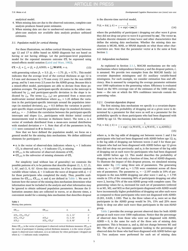
To help connect the concepts of missing data reviewed in the pre-vious section, consider a hypothetical study that was designed to un-derstand if rates of cortical thinning in regions associated with impulsecontrol from ages 12 to 17 differed for those children who had beendiagnosed with ADHD before age 12 from those who had not been di-agnosed. The study was able to recruit 200 12-year-old children to befollowed for 5 years. At baseline, half of the 200 participants had beendiagnosed with ADHD whereas the other half had not been diagnosedwith ADHD. Furthermore, 50 children in each of the two groups hadone or more siblings at the time of recruitment while the other 50children in each group had no siblings by age 12. The study designincluded three waves of data collection, at ages 12, 14.5, and 17. Foreach study participant, define the following data elements:

• CTi = (CTi1, CTi2, CTi3)′ is the cortical thinning complete-datavector for child i (one can think of this as the data that is possible toobserve, though elements are sometimes missing).

• AGEi = (12, 14.5, 17)′ is the age vector that corresponds to CTi.

• WAVEi = (0, 1, 2)′ is the wave vector that corresponds to the datacollection wave.

• ADHDi is a baseline binary variable where ADHDi = 1 for ADHDdiagnosis before age 12 and 0 otherwise.

• SIBi is a baseline binary variable where SIBi = 1 for children whohave siblings by age 12 and 0 otherwise.

Using this hypothetical study, we simulated longitudinal data froma known cortical thinning population model and a variety of knownmissing data mechanisms. While the cortical thinning population modelwas the same for all simulations, we considered four missing datamechanisms that span MCAR, MAR, and MNAR. Elements of the gen-erated data were used to highlight when complete-case analysis andavailable data analysis result in correct inference about the populationparameters for cortical thinning. It is important to note that the ex-amples provided here are not exhaustive but are meant to highlight thefollowing key issues:

1. When missing data are covariate-dependent, both the complete-caseanalysis and available data analysis are unbiased when the correctanalytical model is specified.

2. When missing data are covariate-dependent, omission of that cov-ariate in the analytical model results in two forms of bias, (a) biasdue to the non-independence of the missing data indicator and theoutcome, and (b) omitted variable biased.

3. When missing data are due to, in part, a variable unrelated to theoutcome, that variable is not required to be included in the

T.H. Matta et al. Developmental Cognitive Neuroscience xxx (xxxx) xxx–xxx

4

analytical model.4. When missing data are due to the observed outcomes, complete-case

analysis produces biased point estimates.5. When missing data are due to unobserved outcomes, neither com-

plete-case analysis nor available data analysis produce unbiasedestimates.

3.1. Population model for cortical thinning

For these illustrations, we define cortical thinning (in mm) betweenage 12 and 17 to differ based on ADHD diagnosis but not based onhaving or not having siblings. Let the participant-level populationmodel for the repeated measures outcome CTi be expressed usingmixed-effects model notation (Laird and Ware, 1982),

= + + + + + ϵβ ζ β β ζCT WAVE( ADHD ) .i i i i i i1 1 2 3 2 (13)

with generating values: β1 = 5.5 ; β2 =−1.75 ; β3 = 0.75 ;. This modelindicates that the average level of the cortical thickness at age 12 is5.5 mm and decreases by 1.75 mm every 2.5 years for the non-ADHDgroup, and by 1 mm every 2.5 years for the ADHD group. Because this isa mixed-effect model, participants are able to deviate from these po-pulation averages. The participant-specific deviation in the intercept isindicated by ζ1i and participant-specific deviation in the slope is in-dicated by ζ2i. The terms (ζ1i, ζ2i) are generated from a mean-zeromultivariate normal distribution where ψ11 = 1.25 defines the varia-tion in the participant-specific intercepts around the population inter-cept (in standard deviates), ψ22 = 0.5 defines the variation in partici-pant-specific slopes around the population slope (in standard deviates),and ρ21 =− .3 defines the correlation between the participant-specificintercepts and slopes (i.e., participants with thicker initial corticalmeasurements tend to decrease in thickness faster). The term ϵi is avector of residuals distributed from a mean-zero normal distributionwith standard deviation σ= 1. Note that all of the parameters in Eq.(13) were contained in θ in Section 2.

Now that we have defined the population model, we focus on ageneral model for the missing data mechanisms. We define additionalelements for participant i:

• ri is the vector of observed-data indicators where rij = 1 indicatesCTij is observed and rij = 0 indicates CTij is missing.

• CTi,(1) is the subvector of observed elements of CTi.

• CTi,(0) is the subvector of missing elements of CTi.

For simplicity (and without loss of generality) we constrain thepossible patterns of ri to be patterns that describe dropout: (1, 1, 1)′, (1,1, 0)′, and (1, 0, 0)′. Given this constraint, let d be a discrete randomvariable whose values, di = k indicate the wave of dropout with di = Cfor those participants who completed the study. Thus, possible reali-zations for CTi,(1), CTi,(0), ri and di are defined in Table 1. We now il-lustrate how the nature of the missing data mechanism determines whatinformation must be included in the analysis and what information maybe ignored to obtain unbiased population parameters. Because the il-lustration assumes data are collected in waves, or at discrete times, aconvenient model for a missing data mechanism that describes dropout

is the discrete-time survival model,

= ≥ =+ − ′αw

d k d kℙ( | ) 11 exp( ( ))i i

i (14)

where the probability of participant i dropping out after wave k giventhey did not drop out prior to wave k is governed by ′αwi . The vector wiincludes discrete elements of time/wave and other characteristics thatdefine the missing data mechanism. Whether the missing data me-chanism is MCAR, MAR, or MNAR depends on what those other char-acteristics are. Note that the parameter vector α is the same α fromSection 2.

3.2. Independent mechanisms

As explained in Section 2.1.1, MACAR mechanisms are the onlymechanisms where independence between y and the dropout pattern, r,is assumed. We provide two examples from the MACAR family: (a)covariate dependent missingness and (b) auxiliary variable-basedmissingness. For each example, we consider estimation bias and effi-ciency. Bias is assessed by comparing the average parameter estimatesover 1000 replications to the generating values. Efficiency is evaluatedbased on the 95% coverage rate of the estimates of the 1000 replica-tions — the rate at which the 95% confidence intervals contain thegenerating value.

3.2.1. Covariate-dependent dropoutThe first missing data mechanism we specify is a covariate-depen-

dent one where the probability of dropping out at a given wave is de-termined by a parameter for that wave as well as a parameter for theprobability specific to those participants who had been diagnosed withADHD by age 12. The missing data mechanism is defined as:

= ≥ =+ − + +

d k d kα α α

ℙ( | ) 11 exp( ( WAVE WAVE ADHD ))i i

i1 2 2 3 3

(15)

where α1 is the log odds of dropping out between waves 1 and 2 forparticipants who had not been diagnosed with ADHD before age 12; α2is the log odds of dropping out between waves 2 and 3 for those par-ticipants who had not been diagnosed with ADHD before age 12 giventhey did not drop out previously; and α3 is the increase of the log oddsof dropping out at each wave for participants who had been diagnosedwith ADHD before age 12. This model describes the probability ofdropping out to be not only a function of time, but of ADHD diagnosis.To illustrate the impact of this dropout process, we simulated missingdata under Eq. (15) using three sets of parameters. The generatingvalues α1 =−2.197 and α2 = 1.735 were consistent across all threesets of parameters. The parameter α1 =−2.197 results in 10% of par-ticipants in the non-ADHD dropping out after wave 1 and α2 = 1.735results in 15% of the remaining 90% of participants dropping out afterwave 2, leaving 75% of the non-ADHD group with complete cases. Thegenerating values for α3 increased for each set of parameters (referredto as M1, M2, and M3) so that participants diagnosed with ADHD wouldhave incrementally higher probabilities of dropping out after each waveas compared to those participants who were not diagnosed with ADHD:(0.201, 0.620, 1.100). That is, the three values of α3 were set so thatparticipants in the ADHD group would be 5%, 15% and 25% morelikely to drop out after each wave than participants in the non-ADADgroup.

Table 2 provides the average percent observed data for both ADHDgroups at each wave over 1000 replications. Notice that the percentageof observed data from those who were not diagnosed with ADHD,ADHD = 0, is the same for each of the three sets of missing dataparameters. This is because α1 and α2 did not change between M1 andM3. The effect of α3 becomes apparent looking to the percentage ofobserved data for those who had been diagnosed with ADHD before age12. Two analyses were performed for each set of missing data

Table 1Missing data patterns.

CTi,(1) CTi,(0) ri di

(CTi1, CTi2, CTi3)′ – (1, 1, 1)′ C(CTi1, CTi2)′ (CTi3) (1, 1, 0)′ 2(CTi1) (CTi2, CTi3)′ (1, 0, 0)′ 1

Notes: CTi,(1) is the vector of participant i's observed cortical thickness measures. CTi,(0) isthe vector of participant i's missing cortical thickness measures. ri is the vector of parti-cipant i's observed score indicators. di is an indicator for when participant i dropped outwhere di = C indicates study completion.

T.H. Matta et al. Developmental Cognitive Neuroscience xxx (xxxx) xxx–xxx

5

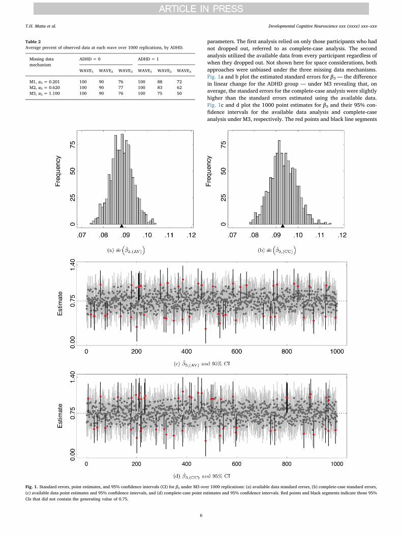
parameters. The first analysis relied on only those participants who hadnot dropped out, referred to as complete-case analysis. The secondanalysis utilized the available data from every participant regardless ofwhen they dropped out. Not shown here for space considerations, bothapproaches were unbiased under the three missing data mechanisms.Fig. 1a and b plot the estimated standard errors for β3 — the differencein linear change for the ADHD group — under M3 revealing that, onaverage, the standard errors for the complete-case analysis were slightlyhigher than the standard errors estimated using the available data.Fig. 1c and d plot the 1000 point estimates for β3 and their 95% con-fidence intervals for the available data analysis and complete-caseanalysis under M3, respectively. The red points and black line segments

Table 2Average percent of observed data at each wave over 1000 replications, by ADHD.

Missing datamechanism

ADHD = 0 ADHD = 1

WAVE1 WAVE2 WAVE3 WAVE1 WAVE2 WAVE3

M1, α3 = 0.201 100 90 76 100 88 72M2, α3 = 0.620 100 90 77 100 83 62M3, α3 = 1.100 100 90 76 100 75 50

Fig. 1. Standard errors, point estimates, and 95% confidence intervals (CI) for β3 under M3 over 1000 replications: (a) available data standard errors, (b) complete-case standard errors,(c) available data point estimates and 95% confidence intervals, and (d) complete-case point estimates and 95% confidence intervals. Red points and black segments indicate those 95%CIs that did not contain the generating value of 0.75.

T.H. Matta et al. Developmental Cognitive Neuroscience xxx (xxxx) xxx–xxx

6

indicate those replicates where the 95% CI did not contain the gen-erating value. Despite the complete-case analysis producing higherstandard errors, the 95% coverage rate for both analyses were 0.95meaning that the complete-case and available data standard errors werewell estimated.

A follow-up simulation was conducted to illustrate the consequenceof omitting a covariate from the analytical model for which the missingdata depends. For this, we generated data under the population model,Eq. (13), and imposed the missing data mechanism from the previousexample. Instead of fitting the correct model, a knowingly misspecifiedmodel for CT was fit to the available data, one that omits ADHDi.

= + + + + ϵβ ζ β ζCT WAVE( ) .i i i i i1 1 2 2 (16)

Table 3 reveals bias in the slope parameter, β2, the slope variance ψ22,and the correlation between the random intercepts and slopes, ρ21,compared to their generating values. However, much of this bias shouldnot be attributed to the dependence between CTi and ri, but instead,attributed to the omission of ADHD, often referred to as omitted variablebias. Because we ignore ADHDi, β2 under the misspecified model is thecompletely pooled linear change for the entire sample, (−1.75 +−1)/2 =1.375. This pooling extends to the linear slope variance componentand the covariance, resulting in a standard deviation of 0.625 andcorrelation of 0.22. Given these pooled estimates, only the slope para-meter exhibits bias due to the missing data under M2 and M3. Analysisof the available data under the most extreme missing data mechanism,M3, where the overall proportion of completers for the ADHD partici-pants was half that of the non-ADHD group, resulted in 4.2% bias due tothe dependence between CT and r. The bias for M3 is closer to thegenerating value of β2 because there were fewer participants in theADHD group resulting in less information to pool towards the gen-erating value of β3.

3.2.2. Auxiliary variable dropoutAnother potential missing data mechanism is one where dropout is

determined by an auxiliary variable — a variable that is not associatedwith the outcome measure. For this example, the probability of drop-ping out increased for those participants with one or more siblings atthe start of the study, perhaps due to scheduling difficulties for parentswith larger families. That is, the auxiliary variable is SIBi because it isindependent of the population model for CTi. Using the discrete-timesurvival model from above, we define the dropout process as

= ≥ =+ − + +

d k d kα α α

ℙ( | ) 11 exp( ( WAVE WAVE SIB ))i i

i1 2 2 3 3

(17)

where the values for α1, α2, and α3 are the same as in Section 3.2.1.What is different is that instead of α3 corresponding from ADHDi, it nowcorresponds to SIBi. Because of our study design, the proportion ofmissing data at each wave by group is equivalent (within replicationvariance) to that of Table 2. Note that this is not quite an example of aMACAR mechanism as defined in Eq. (2) because dropout is still de-pendent on time (WAVE). We know cortical thinning is independent ofhaving one or more siblings but the probability of dropout is not. Asseen in Table 4, because CTi and SIBi are independent, we can ignoreSIB in our model for CTi and obtain the corrected point estimates.

Although the rate of attrition varies, at times drastically, between thetwo groups, Table 4 confirms that (a) ignoring SIBi in the model for CTi

resulted in correct point estimates for parameters for CTi, and (b) bothavailable data and complete-case approaches worked equally well forobtaining those point estimates. Furthermore, with the the most severemissing data condition, coverage rates for both analyses were within1%.

3.3. Ignorable and non-ignorable mechanisms

Like the two examples above, we use Eq. (14) to simulate a MAARand a MNAAR missing data mechanism. The MAAR and MANARmissing data mechanisms are inherently different from the twoMACAR-family missing data processes used above, however, as theyspecify the probability of missing to be a function of CTi. For the re-maining two examples, rather than use CTij directly, we use

= −★CT CT CTjij ij , a mean-centered transformation at each wave. Amissing data mechanism that produces data that are missing at randomis one that depends on the observed cortical thinning measures, CTi,(1).We specify a rather simple MAAR mechanism that generates theprobability of dropping out after each wave to depend on, in part, themeasure of cortical thickness at that wave. That is, the measure ofcortical thickness collected at time k influences whether or not thatparticipant will return at the next wave.

= ≥ =+ − + + ★

d k d kα α α

ℙ( | ) 11 exp( ( WAVE WAVE CT ))i i

1 2 2 3 3 ik

(18)

The MNAAR mechanism is setup just as the MAAR mechanism, onlyinstead of specifying the probability of dropping out after wave k todepend on ★CTik, we use +

★CTi k, 1, or the measure that would have beencollected at the following wave. This formulation results in missing datadue to the cortical thinning measures we do not have.

= ≥ =+ − + + +

★d k d k

α α αℙ( | ) 1

1 exp( ( WAVE WAVE CT ))i ii k1 2 2 3 3 , 1

(19)

This model describes the probability of dropping out after wave k(given that the participant did not drop out prior to wave k) as in-creasing due to growth in cortical thickness after ★CTik is collected. Inorder to enhance our understanding of the impact of ignorable and non-ignorable mechanisms on parameter estimates, both the MAAR andMNAAR simulations were setup differently than the simulations inSections 3.2.1 and 3.2.2. The generating values for α1 and α2 in bothmodels were−2.197 and−1.735, respectively, whereas the generatingvalue for α3 in both models was randomly sampled from a uniformdistribution between 0 and 1.25 over 5000 replications. This strategyenables us to understand the impact of +

★CTi k, 1 on parameter estimatesas a smooth function rather than at select discrete values.

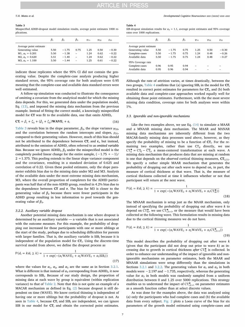
As was done for the examples above, the data was analyzed using(a) only the participants who had complete cases and (b) the availabledata from every subject. Fig. 2 plots a Loess curve of the bias for sixparameters of the growth model estimated using complete-cases and

Table 3Misspecified ADHD-dropout model simulation results, average point estimates 1000 re-plications.

β1 β2 β3 ψ11 ψ22 ρ21

Average point estimateGenerating value 5.50 −1.75 0.75 1.25 0.50 −0.30M1, α3 = 0.201 5.50 −1.38 – 1.24 0.62 −0.22M2, α3 = 0.620 5.51 −1.40 – 1.24 0.62 −0.22M3, α3 = 1.100 5.50 −1.44 – 1.25 0.61 −0.22

Table 4SIB-dropout simulation results for α3 = 1.1, average point estimates and 95% coveragerates over 1000 replications.

β1 β2 β3 ψ11 ψ22 ρ21

Average point estimateGenerating value 5.50 −1.75 0.75 1.25 0.50 −0.30Complete-cases 5.50 −1.75 0.75 1.24 0.48 −0.26Available data 5.50 −1.75 0.75 1.24 0.48 −0.27

95% Coverage rateComplete-cases 0.96 0.95 0.94 – – –Available data 0.95 0.96 0.94 – – –

T.H. Matta et al. Developmental Cognitive Neuroscience xxx (xxxx) xxx–xxx

7

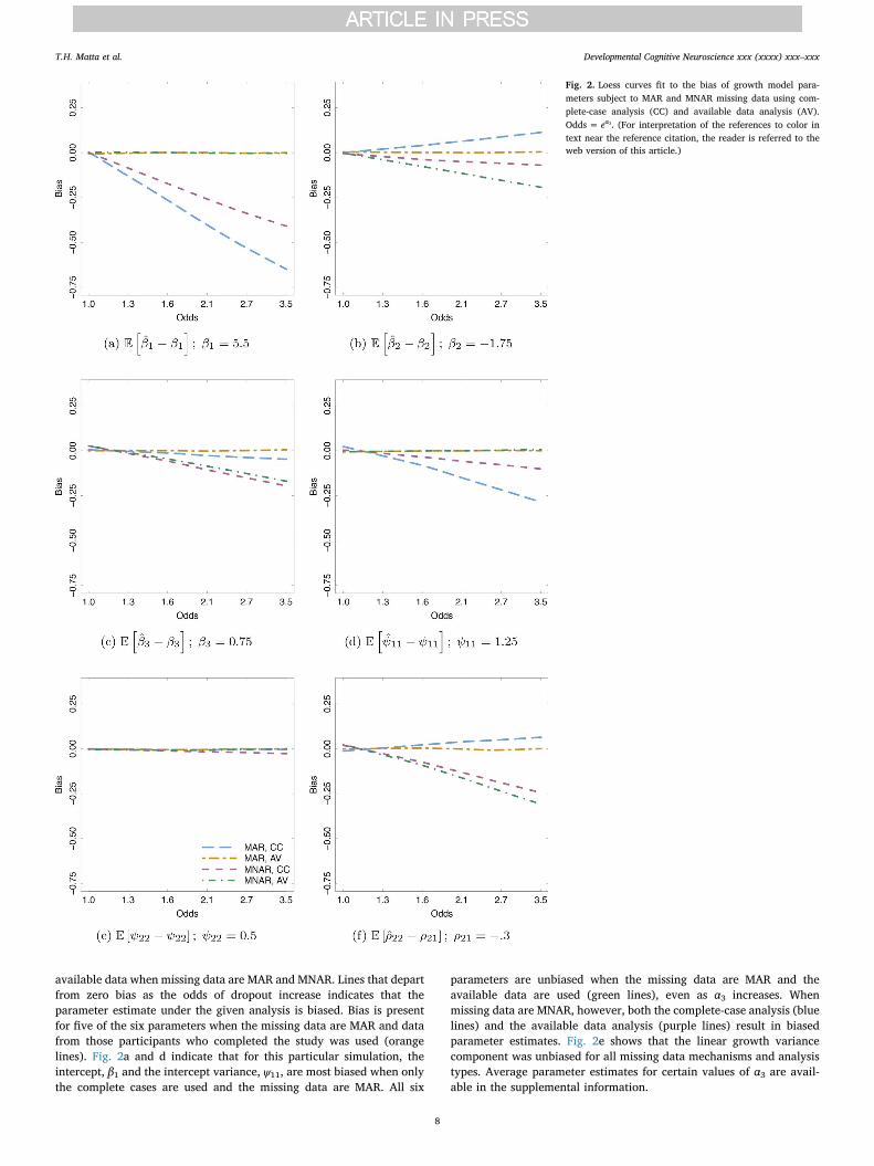
available data when missing data are MAR and MNAR. Lines that departfrom zero bias as the odds of dropout increase indicates that theparameter estimate under the given analysis is biased. Bias is presentfor five of the six parameters when the missing data are MAR and datafrom those participants who completed the study was used (orangelines). Fig. 2a and d indicate that for this particular simulation, theintercept, β1 and the intercept variance, ψ11, are most biased when onlythe complete cases are used and the missing data are MAR. All six

parameters are unbiased when the missing data are MAR and theavailable data are used (green lines), even as α3 increases. Whenmissing data are MNAR, however, both the complete-case analysis (bluelines) and the available data analysis (purple lines) result in biasedparameter estimates. Fig. 2e shows that the linear growth variancecomponent was unbiased for all missing data mechanisms and analysistypes. Average parameter estimates for certain values of α3 are avail-able in the supplemental information.

Fig. 2. Loess curves fit to the bias of growth model para-meters subject to MAR and MNAR missing data using com-plete-case analysis (CC) and available data analysis (AV).Odds = eα3. (For interpretation of the references to color intext near the reference citation, the reader is referred to theweb version of this article.)

T.H. Matta et al. Developmental Cognitive Neuroscience xxx (xxxx) xxx–xxx

8

4. Longitudinal neuroimaging illustrations

The previous section analyzed simulated data from known missingdata mechanisms to demonstrate some of the issues that arise whenanalyzing incomplete data. Whereas simulations rely on known missingdata mechanisms, we can never be sure of the missing data mechanismthat underlies data collected during a study. Therefore, we transition tothe reanalysis of two existing longitudinal neuroimaging datasets, onefunctional and one structural. Specifically, we focus on the sensitivity ofparameter estimates under various missing data assumptions. For bothdatasets, the first analysis exploited the available measures from allparticipants, an operationalization of the MAR assumption, while thesecond analysis employed the data from only those participants whowere measured at all waves, an operationalization of the MCAR as-sumption. Our aim was to compare the sensitivity of estimates betweenavailable and complete data, which has not yet been done with long-itudinal neuroimaging data. This is critical at this stage of the fieldbecause illustrating these differences may have a profound impact onhow developmental cognitive neuroscientists analyze and interpretlongitudinal neuroimaging data. For both datasets, we assessed thesensitivity of the parameter estimates to missing data assumptions byexamining the number and extent of statistically significant clusters inthe first example, and the number of statistically significant parcels inthe second example. Because we are focused on the difference betweenavailable and complete-case data analyses, we are assessing the sensi-tivity of potential ignorable missing data mechanisms. Recall thatMCAR is a special case of MAR, and complete-case analysis is only validwhen missing data are MCAR. That is, if the missing data are MCAR,both analysis of the available data and analysis of the complete caseswill produce similar point estimates while the available data analysis issure to have greater statistical power. The difference in statistical powermay result in different findings under null hypothesis significancetesting. If, however, the missing data are not MCAR, the estimatesproduced by the two approaches will show substantial differences. It isimportant to emphasize that the analyses within this paper do not assessthe sensitivity of parameter estimates to nonignorable missing datamechanisms, which will be taken up in the discussion.

4.1. Task-based functional MRI

4.1.1. Study designThe first example is from a study of the development of self-refer-

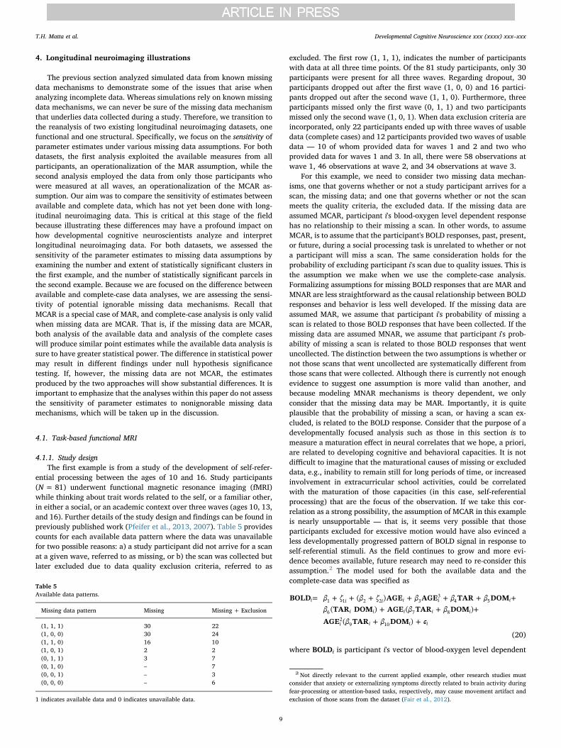
ential processing between the ages of 10 and 16. Study participants(N = 81) underwent functional magnetic resonance imaging (fMRI)while thinking about trait words related to the self, or a familiar other,in either a social, or an academic context over three waves (ages 10, 13,and 16). Further details of the study design and findings can be found inpreviously published work (Pfeifer et al., 2013, 2007). Table 5 providescounts for each available data pattern where the data was unavailablefor two possible reasons: a) a study participant did not arrive for a scanat a given wave, referred to as missing, or b) the scan was collected butlater excluded due to data quality exclusion criteria, referred to as

excluded. The first row (1, 1, 1), indicates the number of participantswith data at all three time points. Of the 81 study participants, only 30participants were present for all three waves. Regarding dropout, 30participants dropped out after the first wave (1, 0, 0) and 16 partici-pants dropped out after the second wave (1, 1, 0). Furthermore, threeparticipants missed only the first wave (0, 1, 1) and two participantsmissed only the second wave (1, 0, 1). When data exclusion criteria areincorporated, only 22 participants ended up with three waves of usabledata (complete cases) and 12 participants provided two waves of usabledata — 10 of whom provided data for waves 1 and 2 and two whoprovided data for waves 1 and 3. In all, there were 58 observations atwave 1, 46 observations at wave 2, and 34 observations at wave 3.

For this example, we need to consider two missing data mechan-isms, one that governs whether or not a study participant arrives for ascan, the missing data; and one that governs whether or not the scanmeets the quality criteria, the excluded data. If the missing data areassumed MCAR, participant i's blood-oxygen level dependent responsehas no relationship to their missing a scan. In other words, to assumeMCAR, is to assume that the participant's BOLD responses, past, present,or future, during a social processing task is unrelated to whether or nota participant will miss a scan. The same consideration holds for theprobability of excluding participant i's scan due to quality issues. This isthe assumption we make when we use the complete-case analysis.Formalizing assumptions for missing BOLD responses that are MAR andMNAR are less straightforward as the causal relationship between BOLDresponses and behavior is less well developed. If the missing data areassumed MAR, we assume that participant i's probability of missing ascan is related to those BOLD responses that have been collected. If themissing data are assumed MNAR, we assume that participant i's prob-ability of missing a scan is related to those BOLD responses that wentuncollected. The distinction between the two assumptions is whether ornot those scans that went uncollected are systematically different fromthose scans that were collected. Although there is currently not enoughevidence to suggest one assumption is more valid than another, andbecause modeling MNAR mechanisms is theory dependent, we onlyconsider that the missing data may be MAR. Importantly, it is quiteplausible that the probability of missing a scan, or having a scan ex-cluded, is related to the BOLD response. Consider that the purpose of adevelopmentally focused analysis such as those in this section is tomeasure a maturation effect in neural correlates that we hope, a priori,are related to developing cognitive and behavioral capacities. It is notdifficult to imagine that the maturational causes of missing or excludeddata, e.g., inability to remain still for long periods of time, or increasedinvolvement in extracurricular school activities, could be correlatedwith the maturation of those capacities (in this case, self-referentialprocessing) that are the focus of the observation. If we take this cor-relation as a strong possibility, the assumption of MCAR in this exampleis nearly unsupportable — that is, it seems very possible that thoseparticipants excluded for excessive motion would have also evinced aless developmentally progressed pattern of BOLD signal in response toself-referential stimuli. As the field continues to grow and more evi-dence becomes available, future research may need to re-consider thisassumption.2 The model used for both the available data and thecomplete-case data was specified as

= + + + + + + +

+ + +

+ + ϵ

β ζ β ζ β β ββ β β

β β

BOLD AGE AGE TAR DOMTAR DOM AGE TAR DOM

AGE TAR DOM

( )( ) ( )

( )

i i i i i i

i i i i i

i i i i

1 1 2 2 33

4 5

6 7 82

9 10

(20)

where BOLDi is participant i's vector of blood-oxygen level dependent

Table 5Available data patterns.

Missing data pattern Missing Missing + Exclusion

(1, 1, 1) 30 22(1, 0, 0) 30 24(1, 1, 0) 16 10(1, 0, 1) 2 2(0, 1, 1) 3 7(0, 1, 0) – 7(0, 0, 1) – 3(0, 0, 0) – 6

1 indicates available data and 0 indicates unavailable data.

2 Not directly relevant to the current applied example, other research studies mustconsider that anxiety or externalizing symptoms directly related to brain activity duringfear-processing or attention-based tasks, respectively, may cause movement artifact andexclusion of those scans from the dataset (Fair et al., 2012).

T.H. Matta et al. Developmental Cognitive Neuroscience xxx (xxxx) xxx–xxx

9

responses for a particular voxel for each level of target (self or other)and domain (academic or social) at each wave. AGEi and AGEi

2 arecorresponding vectors of participant i's age and squared age (centeredat 13). DOMi and TARi are contrast-coded vectors for the levels of thedomain and target factors at which the BOLDi responses had beenmeasured. The random effect terms for the intercept and age effectζ ζ( , )i i1 2 are assumed to be distributed multivariate normal with zeromean and unstructured covariance matrix Psi. The residual term ϵi isassumed to be normally distributed with zero mean and constant var-iance σ The data were analyzed using 3dLME in AFNI (Chen et al.,2013, version 17.0.16;][) and cluster-level significance (pc < .05) wasdetermined using spatial smoothness estimates across all ϵ calculatedby 3dFWHMx (using the acf flag) and Monte-Carlo simulation as im-plemented in 3dClustSim. Whereas the model for the available datauses all 138 observations across three waves, only 66 observations fromthe 22 complete cases were used for the complete-case analysis. Theresults below focus on the sensitivity of β4, the difference in BOLD whilethinking about one's self verses a familiar other at age 13, at the averageof the domain effect. Although this parameter carries an age-specificinterpretation, its estimate is influenced by the longitudinal data. Fur-thermore, this estimate would be used for calculations of the averageand subject-specific BOLD responses across the entire time horizon, soits sensitivity to missing data is just as important as those parametersthat characterize, or interact with, time-specific variables.

4.1.2. ResultsRegarding the number and extent of clusters in the two analyses,

α = .05 was the probability that one or more clusters as big or biggerthan the cut-off would be produced by random spatial noise. For boththe complete-case analysis and the available data analysis, the cluster-defining threshold was p < 0.005. To be considered a significantfinding (i.e., pc < α) under the complete-case analysis, a cluster had tocomprise 270 or more contiguous voxels. For the available data, acluster had to comprise 274 or more contiguous voxels.

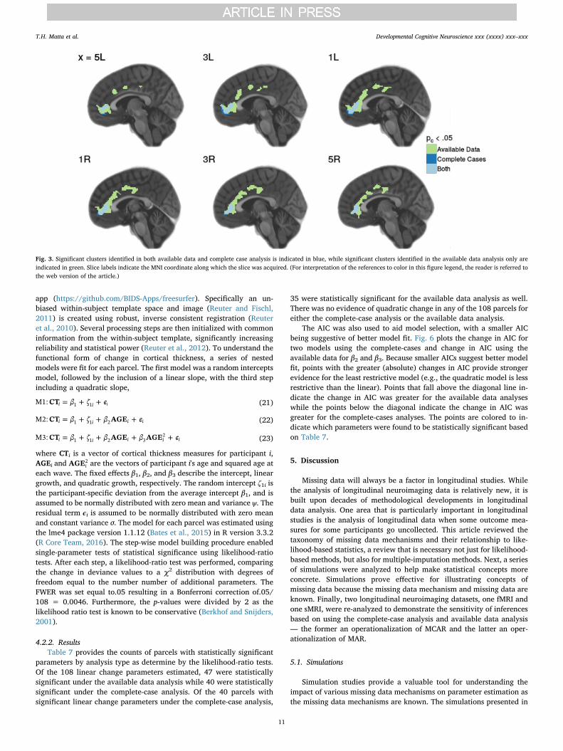
Table 6 indicates that analysis of the available data resulted in theidentification of three clusters, with extents of 1043 voxels (cluster 1),696 voxels (cluster 2), and 280 voxels (cluster 3). In the complete-caseanalysis, we reject the null hypothesis for a single, 312-voxel cluster.The single complete-case cluster shared 274 voxels with cluster 1 fromthe available data analysis. The two remaining clusters identified by theavailable data analysis, one consisting of 696 voxels and the otherconsisting of 280 voxels, went unidentified in the complete-case ana-lysis. Fig. 3 visualizes those significant clusters pertaining to where β4was statistically significant for the available data analysis and thecomplete-case analysis.

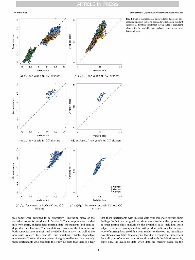
Fig. 4 contains six plots. The first column of plots plot the pairs ofpoint estimates, β β( ˆ , ˆ )v v4 ,(CC) 4 ,(AV) for those voxels that contributed to thesignificant clusters based on (a) the available data only, (c) the com-plete-cases only, and (e) both the available data and complete-cases.The second column of plots plot the pairs of standard errors,

β β(se( ˆ ), se( ˆ ))v v4 ,(CC) 4 ,(AV) for those voxels that contributed to the sig-nificant clusters in the (b) available data analysis only, (d) complete-case analysis only, and (f) both analyses. Along the y-axis for each plotare the estimates from the complete-case analysis and along the x-axisare the estimates from the available data analysis. A point that fall on

the 45-degree line indicates no difference in a voxel's estimate betweenthe two analyses; a point that falls above the line indicates that thevoxel's estimate was larger for the complete-case analysis; and a pointthat falls below the line indicates that the voxel's estimate was be largerfor the available data analysis.

Fig. 4a shows that there was an increase in the available data esti-mates β v4 ,(CC), compared to the complete-case estimates, β v4 ,(CC), for amajority of the voxels the comprised cluster 1 as identified by theavailable data analysis. Furthermore, Fig. 4b shows that the standarderrors for those voxels under the complete-case analysis were, in total,larger than the standard errors produced by the available data analysis.Fig. 4a further indicates that many of the voxel identified in cluster 2were similar in size for the complete-case analysis and available dataanalysis. The standard errors for the cluster 2 voxels were larger underthe complete-case analysis, likely being the reason the cluster wentunidentified in the complete-case analysis. The third cluster under theavailable data had similar characteristics as the first cluster, many ofthe point estimates were larger under the available data analysis andthe available data standard errors were smaller. Fig. 4c indicates thatthose 38 voxels identified by the complete case analysis had largerpoint estimates and Fig. 4d indicates they also had larger standard er-rors. The increase in the standard error was not great enough to counterthe increase in the point estimates. Similarly, Fig. 4c shows that thepoint estimates of the voxels that were contributed to cluster 1 for theavailable data and the complete-case analysis, were similar in size orlarger in size for the complete-case analysis while Fig. 4d indicates thestandard errors were larger for the complete case-analysis. Becausethese were the voxels with the largest cluster 1 point estimates, theincreased standard error, even when there was no change betweenanalyses, enabled them to be identified by the complete-case analysis.

4.2. Surface-based structural MRI

4.2.1. Study designThe enhanced Nathan Kline Institute-Rockland Sample (NKI-RS) is

an ongoing study with the goal of creating a large-scale, communitylifespan sample (details specified by Nooner et al., 2012). The studyemploys a cohort-sequential design where the repeated measures frommultiple age cohorts are linked to create a common developmentaltrend. The present analysis utilizes those subjects that make up a de-velopmental trend from ages 6 through 22, inclusive. The resulting datapattern can be seen in Fig. 5. Since this study is an accelerated long-itudinal design, we compared the available date analysis (using alldata) to an analysis that discards any participant with fewer than twomeasurements taken at least 30 days apart, which mimics the mis-conception that participants with data at just a single wave do notmeaningfully contribute to estimates in longitudinal designs. For con-sistency, we refer to this reduced sample again as the complete-caseanalysis.

For this example, the missing data mechanism governs the prob-ability that a participant will contribute fewer than two measurementstaken at least 30 days apart. In many respects, these subjects may haveentered the study later than the other participants, and can be con-sidered “missing by design.” While such a process would typically bethe result of an MACAR mechanism, the nature of an acceleratedlongitudinal design complicates this. Here, because participants fromdifferent age-cohorts are entering the study at differing rates, and be-cause each cohort provides weight to different portions of the devel-opmental trend, including or excluding these participants will likelyalter the estimates. If the missing data mechanism is MACAR, we shouldexpect the estimates from the complete-case analysis to be similar to theavailable data analysis. For each participant, at each wave, corticalthickness measures were extracted using the ‘Destrieux’ cortical atlas(Fischl et al., 2004). To extract reliable cortical thickness estimates,images were processed with the longitudinal stream (Reuter et al.,2012) in FreeSurfer as implemented by the Freesurfer recon-all BIDS

Table 6Number of voxels contributing to each cluster estimated from the available data andcomplete-case analyses.

Cluster Available data Complete-cases Both

1 1043 312 2742 696 0 03 280 0 0

Both indicate the number of voxels that were part of a given cluster for both the availabledata analysis and the complete-case analysis.

T.H. Matta et al. Developmental Cognitive Neuroscience xxx (xxxx) xxx–xxx

10

app (https://github.com/BIDS-Apps/freesurfer). Specifically an un-biased within-subject template space and image (Reuter and Fischl,2011) is created using robust, inverse consistent registration (Reuteret al., 2010). Several processing steps are then initialized with commoninformation from the within-subject template, significantly increasingreliability and statistical power (Reuter et al., 2012). To understand thefunctional form of change in cortical thickness, a series of nestedmodels were fit for each parcel. The first model was a random interceptsmodel, followed by the inclusion of a linear slope, with the third stepincluding a quadratic slope,

= + + ϵβ ζCTM1: i i i1 1 (21)

= + + + ϵβ ζ βCT AGEM2: i i i i1 1 2 (22)

= + + + + ϵβ ζ β βCT AGE AGEM3: i i i i i1 1 2 32 (23)

where CTi is a vector of cortical thickness measures for participant i,AGEi and AGEi

2 are the vectors of participant i's age and squared age ateach wave. The fixed effects β1, β2, and β3 describe the intercept, lineargrowth, and quadratic growth, respectively. The random intercept ζ1i isthe participant-specific deviation from the average intercept β1, and isassumed to be normally distributed with zero mean and variance ψ. Theresidual term ϵi is assumed to be normally distributed with zero meanand constant variance σ. The model for each parcel was estimated usingthe lme4 package version 1.1.12 (Bates et al., 2015) in R version 3.3.2(R Core Team, 2016). The step-wise model building procedure enabledsingle-parameter tests of statistical significance using likelihood-ratiotests. After each step, a likelihood-ratio test was performed, comparingthe change in deviance values to a χ2 distribution with degrees offreedom equal to the number number of additional parameters. TheFWER was set equal to.05 resulting in a Bonferroni correction of.05/108 = 0.0046. Furthermore, the p-values were divided by 2 as thelikelihood ratio test is known to be conservative (Berkhof and Snijders,2001).

4.2.2. ResultsTable 7 provides the counts of parcels with statistically significant

parameters by analysis type as determine by the likelihood-ratio tests.Of the 108 linear change parameters estimated, 47 were statisticallysignificant under the available data analysis while 40 were statisticallysignificant under the complete-case analysis. Of the 40 parcels withsignificant linear change parameters under the complete-case analysis,

35 were statistically significant for the available data analysis as well.There was no evidence of quadratic change in any of the 108 parcels foreither the complete-case analysis or the available data analysis.

The AIC was also used to aid model selection, with a smaller AICbeing suggestive of better model fit. Fig. 6 plots the change in AIC fortwo models using the complete-cases and change in AIC using theavailable data for β2 and β3. Because smaller AICs suggest better modelfit, points with the greater (absolute) changes in AIC provide strongerevidence for the least restrictive model (e.g., the quadratic model is lessrestrictive than the linear). Points that fall above the diagonal line in-dicate the change in AIC was greater for the available data analyseswhile the points below the diagonal indicate the change in AIC wasgreater for the complete-cases analyses. The points are colored to in-dicate which parameters were found to be statistically significant basedon Table 7.

5. Discussion

Missing data will always be a factor in longitudinal studies. Whilethe analysis of longitudinal neuroimaging data is relatively new, it isbuilt upon decades of methodological developments in longitudinaldata analysis. One area that is particularly important in longitudinalstudies is the analysis of longitudinal data when some outcome mea-sures for some participants go uncollected. This article reviewed thetaxonomy of missing data mechanisms and their relationship to like-lihood-based statistics, a review that is necessary not just for likelihood-based methods, but also for multiple-imputation methods. Next, a seriesof simulations were analyzed to help make statistical concepts moreconcrete. Simulations prove effective for illustrating concepts ofmissing data because the missing data mechanism and missing data areknown. Finally, two longitudinal neuroimaging datasets, one fMRI andone sMRI, were re-analyzed to demonstrate the sensitivity of inferencesbased on using the complete-case analysis and available data analysis— the former an operationalization of MCAR and the latter an oper-ationalization of MAR.

5.1. Simulations

Simulation studies provide a valuable tool for understanding theimpact of various missing data mechanisms on parameter estimation asthe missing data mechanisms are known. The simulations presented in

Fig. 3. Significant clusters identified in both available data and complete case analysis is indicated in blue, while significant clusters identified in the available data analysis only areindicated in green. Slice labels indicate the MNI coordinate along which the slice was acquired. (For interpretation of the references to color in this figure legend, the reader is referred tothe web version of the article.)

T.H. Matta et al. Developmental Cognitive Neuroscience xxx (xxxx) xxx–xxx

11

this paper were designed to be expository, illustrating many of thestatistical concepts introduced in Section 2. The examples were dividedinto two parts, independent missing data mechanisms and non-in-dependent mechanisms. The simulations focused on the limitations ofboth complete-case analysis and available data analysis as well as thenon-issues related to covariate- and auxiliary variable-dependentmissingness. The fact that many neuroimaging studies are based on onlythose participants who complete the study suggests that there is a fear

that those participants with missing data will somehow corrupt theirfindings. In fact, we designed two simulations to show the opposite tobe true! Basing one's analysis on the available data, including thosesubject who have incomplete data, will produce valid results for moretypes of missing data. We didn’t want readers to develop any unrealisticexceptions of available data analysis, that it will rescue their inferencesfrom all types of missing data. As we showed with the MNAR example,using only the available data when data are missing based on the

Fig. 4. Pairs of complete-case and available data point esti-mates and pairs of complete-case and available data standarderrors of β v4 for those voxels that corresponded to significant

clusters for the available data analysis, complete-case ana-lysis, and both.

T.H. Matta et al. Developmental Cognitive Neuroscience xxx (xxxx) xxx–xxx

12

measures that went uncollected will result in biased estimates. The si-mulations were also designed to help researchers understand whatmissing not at random means from a statistical perspective. Often is thecase that a researcher will claim that data is missing not at randombecause missing data is related to one or more variables in their dataset.The simulations in Section 3.2.1 were designed to show that if a cov-ariate is associated with both the outcome of interest and the missingdata indicator, by including that covariate in the model absolves the

analysis of any problem. Leaving such a variable out of the model, wewent on to show, will result in two sources of bias, bias due to missingdata and omitted variable bias, the later having a potentially greaterimpact on the parameter estimates. Furthermore, we demonstrated thenon-issue of missingness associated with an auxiliary variable — avariable that is not related to the outcome of interest.

5.2. Applied examples

The simulations were designed to be quite general, and did notaddress issues specific to longitudinal neuroimaging data. To makethese issues relevant for longitudinal neuroimaging data, we presentedthe re-analysis of two datasets, one fMRI and one sMRI. These long-itudinal neuroimaging illustrations demonstrated how neuroimagingfindings can be sensitive to the assumptions we make about missingdata. Although we are unable to empirically determine the true missingdata mechanism, we can evaluate the extent to which inferences are

Fig. 5. Age at which data was collected from each of 54 participants. Close or overlapping points indicate reliability acquisitions closely spaced in time.

Table 7Counts of statistically significant parameters.

Available data Complete-cases Both

β2 47 40 35β3 0 0 0

Parameter significance was tested using deviance tests with a Bonferroni correction forFWER = 0.05.

Fig. 6. Difference in AIC from complete-case analysis and available data analysis for β2 and β3. ΔAICMj,Mk = AICMj − AICMk, is the difference in AICs between two models. Here, k isconsidered the restricted model and k is nested within j. M1 is Eq. (21), M2 is Eq. (22), M3 is Eq. (23). The leftmost plot describes the test of the linear versus the intercept-only model; therightmost describes the test of the quadratic versus the linear model. Individual points are coded by color and shape to indicate if a given parameter was statistically significant using alikelihood ratio test.

T.H. Matta et al. Developmental Cognitive Neuroscience xxx (xxxx) xxx–xxx

13

sensitive to different assumptions about the missing data mechanism. Inthis paper, we only considered ignorable missing data mechanisms(MCAR and MAR), and stressed how sensitivity the parameter estimateswere to these assumptions. The fMRI example demonstrated that thenumber of, and size of clusters identified can differ considerably basedon one's missing data assumptions. Assuming that the missing data areMCAR, operationalized by using only the complete-cases, resulted inthe identification of only one, relatively small cluster where there weredifferences in levels of activity in self vs. other social cognition. The lessrestrictive assumption of MAR, operationalized by using all the avail-able data, resulted in the identification of three clusters, one of whichcompletely subsumed the cluster identified using the complete cases. Itis likely a combination of the smaller standard errors and the generalincrease in point estimates that enabled the available data analysis toidentify 769 additional voxels as part of cluster 1. Overall, the voxel-specific change in this fMRI study was not negligible and was sensitiveto missing data treatment. Therefore, because using the available datacovers both MACAR and MAAR missing data mechanisms, as long asthe missing data were not MNAR, the inferences drawn from theavailable data analysis had greater validity. These findings from thefMRI example are especially relevant for future research because theyprovide a more realistic idea of missing data in developmental long-itudinal samples especially, where the data goes missing for two rea-sons: due to participants not arriving for their scan at a given time, ordue to data quality issues (e.g., movement during the scan).Theoretically, these sources of missing data may be driven by differentmissing data mechanisms. If, however, both mechanisms are consideredignorable, as we assumed in our analyses, researchers can move for-ward with analysis using the available outcomes they have collected. Inthe sMRI example, the functional form of cortical thinning was esti-mated over a developmental period of age 6 through 22 using an ac-celerated longitudinal design. We considered the sensitivity of in-ferences when those participants who contributed only one measure (ortwo measures less than 30 days apart) were removed from the study,compared to using their data in the estimation. For both the complete-case analysis and the available data analysis, 35 parcels were found toshow linear decline in cortical thickness between the ages of 6 and 22.The available data analysis resulted in an additional 12 parcels thatshowed significant decline while the complete-case analysis resulted in5 additional parcels that showed significant decline. Those parcels thatdiffered between the available data analysis and the complete-casesanalysis did so because those participants who were removed were nota random subset of the sample. Like the sMRI example, because theavailable data are suitable for all ignorable mechanisms — the in-ferences from the available data were more valid than the complete-case analysis. In our two applied examples, it was clear that limitingdata to only the complete cases restricted the findings. Of course, thespecter of an MNAAR mechanism means that we cannot guarantee thatour MAR assumption is more valid than the mcar assumption. RecallFig. 2, where the estimated slope using the available data had greaterbias when the missing data were MNAR than the estimated slope usingthe complete cases. The simulated findings were a product of the spe-cific missing data mechanisms, and they should not suggest that had themissing data mechanisms in the applied examples been MNAAR thatthe complete-case analysis would be more accurate. Instead, we aresaying that under the assumption that the missing data mechanism isignorable, the available data analysis will be more valid. Furthermore,these examples demonstrate how critical it is for research teams in thisfield to be transparent about how they treat missing longitudinal neu-roimaging data, as inconsistencies can adversely affect reproducibilityefforts.

5.3. Guidelines

As more developmental neuroimaging studies adopt longitudinaldesigns, the field's understanding of the issues associated with

analyzing incomplete data is paramount for fostering quality, re-producible research. Such an understanding is evident based on one'sability to theorize why the missing data went uncollected and relatingthose theories to an appropriate missing data mechanism. Furthermore,when the missing data mechanism is assumed to be ignorable, under-standing is evident through one's use of the available data rather thanjust those study participants with complete data. Finally, understandingis evident by acknowledging that a missing data mechanism based onfactors other than the outcome is largely benign. Given this, we havecome up with three guidelines that should enable developmental neu-roscientists to demonstrate understanding of the issues related tomissing data.

5.3.1. Consider the missing data mechanismWhile MCAR mechanisms can be explicitly tested, they are tested

against the assumption that the data are MAR, an assumption thatcannot be verified. Thus, even tests for MCAR rest on unverifiable as-sumptions. Given this, we believe part of the neurodevelopment re-search enterprise should consist of time spent considering why someparticipants in a particular study miss one or more waves of data col-lection, why others participants drop out altogether, and why somemeasures do not meet quality criteria. As we did in the applied ex-ample, researchers should fit multiple models that vary these assump-tions about the missing data mechanism to understand how sensitiveestimates are to a given assumption. For example, if an MCAR me-chanism is assumed, the available data analysis and the complete-caseanalysis should result in very similar estimates.

5.3.2. Exploit the available dataA missing data mechanism that produces data that are MCAR is the

only mechanism where using the subset of subjects who complete thestudy result in valid inferences. However, the use of the available dataproduces valid (and more precise) estimates when missing data areMCAR or MAR. Thus, removing participants from the analysis becausethey have missing data is only going to hurt the analysis, if not becauseof bias, because of the loss of information resulting in larger standarderrors. Although the available data is insufficient when assumptionsabout the missing data tend toward non-ignorability, it provides thebest solution without specifying a model for the joint distribution of theavailable repeated measures outcome and the observed data indicator.Furthermore, including all participants’ data in analyses is the mostresponsible research practice, given the cost and effort of participantand researcher time during data collection.

5.3.3. Focus on the analysis modelIntuition might lead us to think that estimates will be biased if

missing data are related to one or more participant characteristics. Aswe saw in the simulations, however, if those characteristics are relatedto our outcome, we can indeed obtain unbiased estimates if we includethose variables it in our analytical model. The threat of omitted variablebias should make us keen on including those variables just as much asany threat stemming from covariate-dependent missingness. If thevariables related to the missing data process do not also relate to theoutcome, it does not help our estimates to include them in the analy-tical model. Reasoning that one or more variables have been includedin the analytical model purely because they may be related to miss-ingness in the outcome is a misguided decision.

5.3.4. One mechanism for all voxelsOperating within the massively univariate framework, that is, fitting

the same statistical model to each voxel/parcel, means we also mustspecify one missing data mechanism for all voxels/parcels. For ex-ample, in the context of sMRI, some parcels may show evidence of onemissing data mechanism (e.g., MCAR) while others show evidence ofanother (e.g., MAR). It would be advantageous to specify the model toinclude the least conservative missing data assumption. For example,

T.H. Matta et al. Developmental Cognitive Neuroscience xxx (xxxx) xxx–xxx

14

Fig. 6a shows the change in AIC for some parcels to be equal for thecomplete-case analysis and the available data analysis, while for otherparcels, the change in AIC based on the complete-cases and availabledata suggest different substantive results. If a single model must bechosen, it would be advantageous to choose the model the makes theleast restrictive assumption (in this case, MAR, the available dataanalysis).

5.4. Limitations and future directions

It is important to note that this article has not covered the entirefield of missing data. Although we covered the general missing datahierarchy, we placed a majority of emphasis on likelihood-basedmethods for ignorable missing data mechanisms. As a result, we onlytouched on the issues related to data that are missing not at random.This leads to two topics worthy of future study, (a) the fitting oflongitudinal neuroimaging models for non-ignorable missing data (e.g.,Little, 1995 and (b) conducting sensitivity analyses for missing not atrandom assumptions within a massively univariate framework. Finally,a note on why we chose to focus on likelihood-based methods formissing data. Our first consideration was pedagogical, likelihood-basedmethods have an unambiguous relationship to the missing data hier-archy. Second, multiple imputation was originally developed formissing data problems in survey research where missing data exists onmany variables (Andridge and Little, 2010; Belin and Song, 2014). Inlab settings with tight protocols, where neuroimaging data is beingoriginated, it is more likely to encounter a person with missing data foran entire wave rather than partial missing data at a given wave. Thus,although multiple imputation has proven effective for missing dataproblems outside of survey research, any advantage over maximumlikelihood in such settings would be negligible. Third, although mul-tiple imputation has become a popular tool for handling missing data,longitudinal neuroimaging data in a massively univariate frameworkcreates many complexities. The first complexity is computational, withhundreds of thousands of models being estimated, using, say 10 im-puted datasets would mean estimating ten times an already hugenumber of models. The second complexity is statistical, that is, a validimputation model must considers the this structure of the longitudinaldata — something not so straight forward (Goldstein and Carpenter,2014). That said, we recommend the review by Harel and Zhou (2007)to those readers interested in multiple imputation as a general frame-work for handling missing data.

6. Conclusion

While the guidelines are not exhaustive, we believe adherence tothem will elevate the quality of research in the field. That is, if futurelongitudinal neuroimaging studies exploit all of the available data andfocus on properly specifying their analytical model, they will have fit amodel that provides valid inferences under MCAR and MAR missingdata processes. Reporting these practices transparently will result inhigher rates of reproducibility and overall greater understanding ofbrain development. We hope that as longitudinal studies in develop-mental neuroscience continues to grow, the field does not stop here, butembraces the study of missing data as it relates to neuroimaging data.

Conflict of interest

The authors declare that there is no conflict of interest.

References

Andridge, R.R., Little, R.J.A., 2010. A review of hot deck imputation for survey non-response. Int. Stat. Rev. 78 (1), 40–64.

Bates, D., Mächler, M., Bolker, B., Walker, S., 2015. Fitting linear mixed-effects modelsusing lme4. J. Stat. Softw. 67 (1), 1–48. http://dx.doi.org/10.18637/jss.v067.i01.

Belin, T.R., Song, J., 2014. Missing data in sample surveys. In: Molenberghs, G.,Fitzmaurice, G., Kenward, M.G., Tsiatis, A., Verbeke, G. (Eds.), Handbook of MissingData Methodology. CRC Press, Boca Raton, FL, pp. 525–546.

Berkhof, J., Snijders, T., 2001. Variance component testing in multilevel models. J. Educ.Behav. Stat. 26 (2), 133–152.

Chen, G., Saad, Z.S., Britton, J.C., Pine, D.S., Cox, R.W., 2013. Linear mixed-effectsmodeling approach to FMRI group analysis. NeuroImage 73, 176–190.

Diggle, P., Zeger, S.L., Liang, K., Heagerty, P., 2002. Analysis of Longitudinal Data, 2nded. Oxford University Press, Oxford.

Fair, D.A., Nigg, J.T., Iyer, S., Bathula, D., Mills, K.L., Dosenbach, N.U.F., Schlaggar, B.L.,Mennes, M., Gutman, D., Bangaru, S., Buitelaar, J.K., Dickstein, D.P., Di Martino, A.,Kennedy, D.N., Kelly, C., Luna, B., Schweitzer, J.B., Velanova, K., Wang, Y.F.,Mostofsky, S., Castellanos, F.X., Milham, M.P., 2012. Distinct neural signatures de-tected for adhd subtypes after controlling for micro-movements in resting statefunctional connectivity mri data. Front. Syst. Neurosci. 6 (80). http://dx.doi.org/10.3389/fnsys.2012.00080.

Fischl, B., Van Der Kouwe, A., Destrieux, C., Halgren, E., Ségonne, F., Salat, D.H., Busa, E.,Seidman, L.J., Goldstein, J., Kennedy, D., Caviness, V., Makris, N., Rosen, B., Dale,A.M., 2004. Automatically parcellating the human cerebral cortex. Cereb. Cortex 14(1), 11–22. http://dx.doi.org/10.1093/cercor/bhg087.

Friston, K.J., Holmes, A.P., Worsley, K.J., Poline, J.B., Frackowiak, R.S.J., 1995.Statistical parametric maps in functional imaging: a general linear approach. Hum.Brain Mapping 2 (4), 189–210.

Goldstein, H., Carpenter, J.R., 2014. Multilevel multiple imputation. In: Molenberghs, G.,Fitzmaurice, G., Kenward, M.G., Tsiatis, A., Verbeke, G. (Eds.), Handbook of MissingData Methodology. CRC Press, Boca Raton, FL, pp. 295–316 46.

Gorgolewski, K.J., Poldrack, R.A., 2016. A practical guide for improving transparency andreproducibility in neuroimaging research. PLoS Biol. 14 (7).

Harel, O., Zhou, X.-H., 2007. Multiple imputation: review of theory, implementation andsoftware. Stat. Med. 26, 3057–3077.

Heckman, J.J., 1976. The common structure of statistical sodels of truncation, sampleselection and limited dependent variables and a simple estimator for such models.Ann. Econ. Soc. Meas. 5 (4), 475–492.

Jelicić, H., Phelps, E., Lerner, R.M., 2009. Use of missing data methods in longitudinalstudies: the persistence of bad practices in developmental psychology. Dev. Psychol.45 (4), 1195–1199.

Jennrich, R.I., Schluchter, M.D., 1986. Unbalanced repeated-measures models withstructured covariance matrices. Biometrics 42 (4), 805–820.

Kenward, M., Molenberghs, G., 1998. Likelihood based frequentist inference when dataare missing at random. Stat. Sci. 13 (3), 236–247.

Laird, N.M., 1988. Missing data in longitudinal studies. Stat. Med. 7, 305–315.Laird, N.M., Ware, J.H., 1982. Random-effects models for longitudinal data. Biometrics

38 (4), 963–974.Little, R.J.A., 1976. Inference about means from incomplete multivariate data. Biometrika

63 (3), 593–604.Little, R.J.A., 1993. Pattern-mixture models for multivariate incomplete data. J. Am. Stat.

Assoc. 88 (421), 125–134.Little, R.J.A., 1994. A class of pattern-mixture models for normal incomplete data.

Biometrika 81 (3), 471–483.Little, R.J.A., 1995. Modeling the drop-out mechanism in repeated-measures studies. J.

Am. Stat. Assoc. 90 (431), 1112–1121.Little, R.J.A., 2009. Selection and pattern-mixture models. In: Fitzmaurice, G., Davidian,

M., Verbeke, G., Molenberghs, G. (Eds.), Longitudinal Data Analysis. Chapman &Hal/CRC, Boca Raton, FL, pp. 409–431.

Mealli, F., Rubin, D.B., 2015. Clarifying missing at random and related definitions, 47 andimplications when coupled with exchangeability. Biometrika 102 (4), 995–1000.

Molenberghs, G., Beunckens, C., Sotto, C., Kenward, M.G., 2008. Every missingness not atrandom model has a missingness at random counterpart with equal fit. J. R. Stat. Soc.Ser. B 70, 371–388.

Molenberghs, G., Fitzmaurice, G., 2009. Incomplete data: introduction and Overview. In:Fitzmaurice, G., Davidian, M., Verbeke, G., Molenberghs, G. (Eds.), Longitudinal DataAnalysis. Chapman & Hall/CRC, Boca Raton, FL, pp. 395–408.

Nooner, K., Colcombe, S., Tobe, R., Mennes, M., Benedict, M., Moreno, A., Panek, L.J.,Brown, S., Zavitz, S.T., Li, Q., Sikka, S., Gutman, D., Bangaru, S., Schlachter, R.T.,Kamiel, S.M., Anwar, A.R., Hinz, C.M., Kaplan, M.S., Rachlin, A.B., Adelsberg, S.,Cheung, B., Khanuja, R., Yan, C., Craddock, C.C., Calhoun, V., Courtney, W., King, M.,Wood, D., Cox, C.L., Kelly, A.M., Di Martino, A., Petkova, E., Reiss, P.T., Duan, N.,Thomsen, D., Biswal, B., Coffey, B., Hoptman, M.J., Javitt, D.C., Pomara, N., Sidtis,J.J., Koplewicz, H.S., Castellanos, F.X., Leventhal, B.L., Milham, M.P., 2012. The nki-rockland sample: a model for accelerating the pace of discovery science in psychiatry.Front. Neurosci. 6, 152. http://dx.doi.org/10.3389/fnins.2012.00152.

Pfeifer, J.H., Kahn, L.E., Merchant, J.S., Peake, S.J., Veroude, K., Masten, C.L., Lieberman,M.D., Mazziotta, J.C., Dapretto, M., 2013. Longitudinal change in the neural bases ofadolescent social self-evaluations. Effects Age Pubertal Dev. 33 (17), 7415–7419.http://dx.doi.org/10.1523/JNEUROSCI.4074-12.2013.

Pfeifer, J.H., Lieberman, M.D., Dapretto, M., 2007. I know you are but what am i?! Neuralbases of self-and social knowledge retrieval in children and adults. J. Cogn. Neurosci.19 (8), 1323–1337.

R Core Team, 2016. R: A Language and Environment for Statistical Computing [ComputerSoftware Manual]. Vienna, Austria. Retrieved from https://www.R-project.org/.

Reuter, M., Fischl, B., 2011. Avoiding asymmetry-induced bias in longitudinal imageprocessing. NeuroImage 57 (1), 19–21.

Reuter, M., Rosas, H., Fischl, B., 2010. Highly accurate inverse consistent registration: arobust approach. NeuroImage 53 (4), 1181–1196.

Reuter, M., Schmansky, N., Rosas, H., Fischl, B., 2012. Within-subject template estimationfor unbiased longitudinal image analysis. NeuroImage 61 (4), 1402–1418.

T.H. Matta et al. Developmental Cognitive Neuroscience xxx (xxxx) xxx–xxx

15

Rubin, D.B., 1976. Inference and missing data. Biometrika 63 (3), 581–592.Seaman, S., Galati, J., Jackson, D., Carlin, J., 2013. What is meant by “missing at 48

random”? Stat. Sci. 28 (2), 257–268.Skrondal, A., Rabe-Hesketh, S., 2004. Generalized Latent Variable Modeling. Chapman &

Hall/CRC, Boca Raton, FL.Wang-Clow, F., Lange, M., Laird, N.M., Ware, J.H., 1995. A simulation study of estimators

for the rates of change in longitudinal studies with attrition. Stat. Med. 14 (3),283–297.

Wu, M.C., Carroll, R.J., 1988. Estimation and comparison of changes in the presence ofinformative right censoring by modeling the censoring process? Biometrics 44 (1),175–188.

T.H. Matta et al. Developmental Cognitive Neuroscience xxx (xxxx) xxx–xxx

16