making money with cvar 1. introduction markowitz introduced

MAKING MONEY WITH CVAR

MEMBERS: MARK GLAD, CHEN ZHANG, BOWEN YU, YIRAN ZHANG,FEIYU PANG, HAOCHEN KANG, LIQIONG ZHAO

MENTOR: CHRISTOPHER BEMIS

1. Introduction

Markowitz introduced his pioneering work on Modern Portfolio Theory in 1952.In this mean-variance approach to optimize a given portfolio of assets, he focused onstudying the effects of asset risk, return, correlation and diversification on probableinvestment portfolio returns [1]. In the late 1980s, minimizing Value-at-Risk (VaR)became widely used among financial institutions and became an important way to bothmeasure the risk of a portfolio of financial instruments, and then to allocate the portfolioto minimize that risk. However, VaR lacks sub-additivity (Artzner at al., 1997, 1999).That is, for a non-normal distribution, diversification of the portfolio may increaseVaR. In addition, VaR is a non-convex and non-smooth function of the weights of theindividual positions, and has multiple local extrema. Such features can make it difficultto optimize VaR for a discrete distribution [2]. Because of these disadvantages, a newapproach to measure risk, Conditional Value-at-Risk (CVaR), was developed. CVaR isa coherent measure of risk, and has the benefit of incorporating all of the tail behaviorof the distribution of returns (losses), beyond the minimum loss that is the VaR of theportfolio. CVaR is defined as the expectation of losses that exceed VaR. We implementfour methods to minimize CVaR with respect to the weights of the asset. This allocationis defined as the optimal allocation for this collection of assets. The first method tominimize CVaR is to transfer the original problem to a linear programming problem asconsidered by Rockafellar and Uryasev [3]; the second method is to use a fast gradientdescent method proposed by Iyengar and Ma [4]; the third method is to approximate theloss function with aC1 function, as suggested by Alexander, Coleman and Li [5]; and thefinal method is to approximate the loss function with a smooth convolution of the lossfunction as constructed by Bemis [6]. We compare the efficiency and accuracy of the fourmethods, and use as benchmarks a portfolio allocated by Mean Variance methodology,and the optimal portfolio computed in Rockefellar [3]. Finally we analyze the out ofsample performance of optimal portfolios computed from each these approaches.

1

2. Mean VarianceMethodology, a Benchmark

The main idea of Mean Variance Methodology proposed by Markowitz [1] is shownbelow,

minimize xTΣxsubject to µTx > R

1Tx = 1x > 0,

where x stands for the weights of the assets in the portfolio, Σ is the covariance matrixfor the multivariate normal distribution of the assets, and R denotes the minimumreturn constraint of portfolio. The results from the Mean Variance Methodology canbe used as a comparison for the other four approaches, since at an allocation whenthe constraint for expected minimum return is active, and when β > 0.5, the optimalportfolio allocation from the MV methodology will agree with the optimal portfolioproduced by minimizing CVaR.

Table 1 and Table 2 are the data we borrow from Rockafellar and Uryasev’s paper[3]. According to the Mean Variance Methodology, we calculate the weights of optimalportfolio, VaR and CVaR under different β, as Table 3 and Table 4 show.

3. Linear ProgrammingMethod

Rockafellar and Uryasev [3] introduce a performance function and auxiliary variablesto model the original problem as a linear programming (LP) problem. By discretizating,CVaR is minimized with samples generated from a distribution of scenarios y. In ourpaper, f(x, y) denotes the loss function, where x = [x1, . . . , xN]T denotes a vector ofweights (the weights of assets in the portfolio) and y = [y1, . . . ,yN]T is a vector of thereturns of assets. Let p(y) describe the probability density function of y. The probabilityof f(x, y) not exceeding a threshold is given by

Ψ(x,α) =∫f(x,y)6α

p(y)dy.

Given a certainty level β, VaR and CVaR are defined as

VaRβ = VaRβ(x) = minα ∈ R |Ψ(x,α) > β,

and

CVaRβ = CVaRβ(x) = (1 − β)−1∫f(x,y)>VaRβ(x)

f(x, y)p(y)dy.

It can be proved that β-CVaR associated with any x can be achieved by minimizingthe performance function with respect to α

Fβ(x,α) = α+ (1 − β)−1∫f(x,y)>VaRβ(x)

[f(x, y) − α]+p(y)dy.

2

By discretizing, Fβ(x,α) can be approximated with samples generated from the dis-tribution of y, i.e. yk, k =1, 2, ..., q by

Fβ(x,α) = α+1

q(1 − β)

q∑k=1

[f(x, yk) − α]+.

We use the loss function, f(x, y) = −xTy. With the introduction of auxiliary variablesuk, k = 1, 2, ..., q, we can rewrite the objective function as

Fβ(x,α) = α+1

q(1 − β)

q∑k=1

uk,

with constraints uk > 0 and xTy + α + uk > 0, k = 1, 2, ..., q. Therefore the originalproblem is converted into an linear programming problem and can be presented as

minimize α+1

q(1 − β)

q∑k=1

uk

subject to xTy + α+ uk > 0uk > 0x > 01Tx = 1−µTx 6 −R,

where R denotes the minimum return required for the portfolio.As Rockafellar et al. indicate, the optimal weights obtained from the solution to this

LP problem is the same as those obtained from Modern Portfolio Theory introduced byHarry Markowitz, if (1) the last constraint is active (i.e., µTx = R), (2) β > 0.5, and (3)the returns of assets are multivariate normally distributed.

In order to see the approximation of Rockafellar and Uryasev’s approach, we generatemultivariate normally distributed random values as data in our samples. Also, we wantto see the change in runtime with respect to a change in the number of assets or thenumber of scenarios. As is seen from the results, runtime changes when differentsamples are being used. Thus, we calculate the average runtime for five differentsamples.

In addition, we find that the LP problem solver in MOSEK is dramatically faster thanthe one in MATLAB. Our runtime for Rockafellar and Uryasev’s approach is recordedin terms of MOSEK LP problem solver.

As is shown in Figure 1, runtime goes up rapidly as the number of scenarios increases,while it grows at a relatively constant rate when the number of assets increases. Speedis the downside of this method.

Table 5 indicates that for these three assets (S&P, Gov Bond, Small Cap), longerruntime needs to be allowed to calculate VaR and CVaR, as the number of scenariosincreases under a specific β (β = 0.90, 0.95, 0.99).

3

4. Iterative Gradient DescentMethod

The method proposed by Iyengar and Ma is to compute approximate solutions forthe scenario-based mean-CVaR portfolio selection problem. This procedure is based onan algorithm suggested by Nesterov [7] for solving non-smooth convex optimizationproblems. The basic equation of β-CVaR is defined as follows

CVaRβ(−Yx) = EP[−Yx|Yx 6 F−1Yx (β)],

where x denotes the weight of the portfolio, Y = [y1, · · · , ys] is the scenario matrixgenerated form p(y), −Yx denotes the random variable for the loss of portfolio, and FYxrepresents for the CDF of Yx. As before, β stands for the probability that determines thequantile of CVaR. In general, we choose β equal to 0.90, 0.95 or 0.99 in the Mean-CVaRproblem. According to Iyengar and Ma’s method [5], we use the equivalent formulationof CVaR

CVaRβ(−Yx) = maxQ∈QEQ[Yx],

Q is a probability measure on the returns Y.From this, the scenario-based mean-CVaR problem reduces to the saddle-point prob-

lem

minx∈X

maxq∈Q

−qTYx.

And the restrictions of x and q could be defined as follows

Q = q ∈ Rs : 1T q = 1, 0 6 q 61

1 − βp,

X = x ∈ RN : x > 0,−mTx 6 −R, 1Tx = 1,

where p = [p1, . . . ,ps]T and pi, i = 1, 2, ..., s, denotes the probability of the i-th scenario.The following formulas are the main idea of Nesterov Produce [7] given an error boundε.D1 ← 1

2(1 + 2M)2,M =∞,

D2 ← −11−β(β lnβ+ (1 − β) ln (1 − β)),

σ2 ← 1β , Ω← maxi‖yi‖2

2,

K← 1ε

√ΩD1D2σ2

, µ← ε2D2

,

x(0) ← 1N1, d2(q)←

∑si=1 qi ln qi + ( pi1−β − qi) ln ( pi1−β − qi),

for k← 0 to K, doq(k) ← arg maxq∈Q

qTYx(k) − µd2(q)

,

w(k+1) ← arg minw∈X

−(q(k))TYw(k) + Ω

2µσ2‖w − x(k)‖2

2

,

z(k+1) ← arg minz∈X

−∑kt=0

t+12 q(t)Yz + Ω

2µσ2‖z‖2

2

,

x(k+1) ← 2k+1 z(k+1) + k+1

k+3 w(k+1),

return x∗ = w(K), q∗ =∑Kk=0

2(k+1)(K+1)(K+2) q(k).

4

5. Approximation Approach

As described in Rockafellar [3], minimizing CVaRβ is the optimization problem

minFβ(x,α)(x,α)∈X×R

= α+1

1 − β

∫[−xTy − α]+p(y)dy.

Discretization of it gives the following optimization problem

min(x,α)∈X×R

Fβ(x,α) = α+1

q(1 − β)

q∑j=1

[−xTyj − α]+.

Let h = max(z, 0). The C0 function h can be approximated by functions with higherorder differentiability properties.

5.1. Convolution Method. Bemis et al.(2010) [6] proposed a convolution method thatapproximates the objective function by a smooth function. They convolve the piecewiselinear function h by a mollifier ηε : R→ R

η(z) =

C exp( 1

z2−1), if − 1 < z < 10, otherwise

where C is chosen so that∫∞−∞ η(z)dz = 1. Given a resolution parameter ε, let

ηε(z) =

Cε exp( 1

(z/ε)2−1), if − ε < z < ε

0, otherwise

Then the objective function F can be approximated by smooth functions

φεβ(x,α) := α+1

(1 − β)

∫(ηε ∗ h)(−xTy − α)p(y)dy

= α+1

(1 − β)

∫Rn

∫ε−εηε(−xTy − α− z)h(z)dzdy.

φεβ is smooth and convex. In addition, limε→0

min(x,α)∈X×R

φεβ = minx∈X

CVaR(x).

And equation φεβ can be discretized as

φεβ = α+1

q(1 − β)

q∑j=1

∫Rηε(−xTyj − α− z)[z]+dz

= α+1

q(1 − β)

q∑j=1

∫ 1

−1[−xTyj − α− εz]+η(z)dz

≈ α+1

q(1 − β)

q∑j=1

N∑n=1

ωnη(zn)[−xTyj − α− εz]+,

where zn is the n-th root of the N-th degree legendre polynomial and ωi are thecorresponding weights. The gradient and Hessian of φεβ could also be obtained bynumerically obtain the intergral.

5

5.2. Piecewise Quadratic Approximation. Alexander [4] also proposed a similar ap-proximation method. They suggest an alternative piecewise quadratic polynomialρε : R→ R

ρε(z) =

0, if z 6 −ε

z2

4ε +z2 + ε

4 , if − ε < z < εz, if z > ε

Thus, the equation F is approximated by

Fβ(x,α) = α+1

q(1 − β)

q∑j=1

ρε(−xTy − α),

where (x,α) ∈ X×R.The function F is a continuously differentiable function, and there are various tools

to solve it.

6. Four Approaches Compared withMarkowitz’sMethodology

As has been proved in Rockafellar and Uryasev’s paper, the minimized VaR and CVaRis the same as the VaR and CVaR calculated by minimizing variance using Markowitz’smodern portfolio theory, when (1)β is larger than or equal to 0.5, (2) the returns of assetsfollow multivariate normal distribution, and (3) the constraint of minimum return isactive. Thus, we consider VaR and CVaR calculated from Markowitz’s Mean VarianceApproach as a benchmark to evaluate approximation of the four approaches.

As is shown in Figure 4, both VaR and CVaR calculated from all four methods arerelatively close to our benchmark, when β is below or equal to 0.90.

As β increases, significant difference may occur in the smoothed approximationmethod and the convolution method (Figure 5, 6). This is because as β increases, theprobability of loss exceeding VaR becomes relatively small. When a smooth functionis to be approximated, more samples (i.e., scenarios) are necessary to ensure a betterconvergence. On the other hand, the linear approximation method and the iterativegradient descent method exhibit less sensitivity to the value of β, which can be clearlyseen with VaRs and CVaRs calculated from the smoothed approximation method andthe convolution method removed. We notice that the calculated VaRs and CVaRs do notseem to converge. This is because the scenarios generated by MATLAB are not perfectlynormally distributed and our samples are not large enough.

In addition, runtime of implementation of the four methods is recorded and a com-parison of efficiency is made. As the number of scenarios increases, the time it takes tosolve the linear programming problem increases dramatically. This sacrifices efficiencyfor a better approximation. However, the runtime of the iterative gradient descentmethod only increase gradually. On the other hand, the runtime of the linear program-ming method remains relatively stable as the number of assets increases; however theruntime of the iterative gradient descent method increases significantly in this case. Im-plementations of the smoothed approximation method and the convolution smoothingmethod are fast in both cases. Therefore, we come to the conclusion from Figure 7 thatthe linear programming method is sensitive to the number of scenarios and insensitive

6

to the number of assets, while the iterative gradient descent method is just the otherway around.

7. Out of Sample Performance

In this section, we want to see the effectiveness of the four approaches when applyingthem to the real world. The real data sets are provided by our mentor, Chris Bemis.

Our data sets include over 1000 assets and only 6 month daily returns for thoseassets. We only compare the performance of the linear programming method and theiterative gradient descent method with an evenly weighted investment strategy andmarket capital weighted strategy, because the ”fmincon” function in MATLAB cannotmanage this large number of assets and only 126 scenarios. Comparing our results(Figure 8, 9, 10, 11) with S&P 500 index, we can see that the linear programming methodand the iterative gradient descent method perform better when the market is bad, orgoing down (as in year 2001); the linear programming method and the iterative gradientdescent method perform as good as the other two strategies (as in year 2002); the linearprogramming method and the iterative gradient descent method perform badly whenthe market is good, or going up (as in year 2003).

One of reasons might be that CVaR functions differently from variance in terms ofbeing a risk measure. While variance can measure both ”good” risk (i.e., the situationthat the market may go extremely well) and ”bad” risk (i.e., the situation that themarket may go unexpectedly bad), just like volatility (i.e., ups and downs), CVaR, asa measure of loss, is more or less like a measure of ”bad” risk. That is the reasonwhy we see better performance of the CVaR minimization methods (i.e., the linearprogramming method and the iterative gradient descent method) when the market isbad, but worse performance in a good market, in which case we tend to be conservativein investing when trying to minimizing CVaR, or loss. We even see the large volatilityin the performance of the iterative gradient descent method in year 2003, which mightbe avoided if we minimize variance instead of minimizing the average of the largest 1 -β percent of loss, or CVaR.

Another reason might be that as time goes by, the mean return of each asset changes,which means using the same strategy for the whole year is unfair. The weights of assetsin the portfolio may need to be adjusted.

We did not test the smoothed approximation method and the convolution method inthe case of real data, because those two methods require a extremely large number ofscenarios given more than 1000 assets. It is simply unrealistic to use data of such a longperiod of time. One solution might be that we simulate scenarios in addition to the 126actual data points. Another solution is that we narrow down the number of assets inthe portfolio and then apply all four models to a smaller number of assets.

7

AcknowledgementWe would like to express our gratitude to all those who gave us the possibility to

complete this project. We want to thank the Institute of Mathematics and its Application.We are also deeply indebted to our Mentor, Christopher Bemis, whose help, stimulatingsuggestions and encouragement helped us in all the time of research for this project.

References:[1] Markowitz, H.M. (1959). Portfolio Selection: Efficient Diversification of Invest-

ments.[2] Pavlo Krokhmal, Jonas Palmquist, and Stanislav Uryasev, Portfolio Optimization

with Conditional Value-at-Risk Objective and Constraints, September 25, 2001.[3] R.T. Rockafellar and S. Uryasev, Optimization of Conditional Value-At-Risk. The

Journal of Risk, Vol. 2, No. 3, pp. 21-41, 2000.[4] S. Alexander, T. F. Coleman, and Y. Li, Minimizing VaR and CVaR for a Portfolio

of Derivatives, Journal of Banking and Finance, Vol. 30, no. 2, pp. 583-605, 2006.[5] G. Iyengar and A.K.C. Ma, Fast gradient descent method for mean-CVaR opti-

mization, 2009, preprint.[6] Chris Bemis, Yifei Chen, Holly Chung, Fernando Fontove, Daniel Jordon, Heng

Ye, A Study in CVaR Optimization and Joint Density Modeling, August 25, 2010.[7] Y. Nesterov. Smooth minimization of non-smooth functions. Mathematical Pro-

gramming, 103 (1):127-152, May 2005.

8

Appendix

9

Table 1. Portfolio Mean Returns

Instrument Mean ReturnS&P 0.010111

Gov Bond 0.0043532Small Cap 0.0137058

Table 2. Portfolio Covariance Matrix

S&P Gov Bond Small CapS&P 0.00324625 0.00022983 0.00420395

Gov Bond 0.00022983 0.00049937 0.00019247Small Cap 0.00420395 0.00019247 0.00764097

Table 3. Optimal Portfolio with the Mean Variance Approach

S&P Gov Bond Small Cap0.452011311 0.115573182 0.432415507

Table 4. VaR and CVaR obtained with the Mean Variance Approach

β = 0.9 β = 0.95 β = 0.99VaR 0.067847077 0.090199128 0.132127858

CVaR 0.096974824 0.115907789 0.152976508

10

Table 5. The Performance of Linear Programming Method

β Smpls S&P Gov Small VaR VaR CVaR CVaR Runtime# Bond Cap Dif (%) Dif (%) (cputime)

0.90 1000 0.66478 0.03379 0.30143 0.06 6.72 0.09 4.60 0.080.90 2000 0.47377 0.10721 0.41902 0.07 2.08 0.09 2.81 0.280.90 3000 0.45981 0.11257 0.42761 0.07 0.51 0.10 0.96 0.580.90 4000 0.48310 0.10362 0.41328 0.07 0.36 0.10 0.66 1.030.90 5000 0.45389 0.11485 0.43126 0.07 1.20 0.10 1.04 1.610.90 6000 0.43780 0.12103 0.44116 0.07 2.40 0.10 1.03 2.260.90 7000 0.45756 0.11344 0.42900 0.07 4.15 0.10 4.17 3.090.90 8000 0.46236 0.11160 0.42605 0.07 1.28 0.10 0.13 3.990.95 1000 0.33239 0.16155 0.50606 0.09 0.48 0.12 1.56 0.090.95 2000 0.20880 0.20906 0.58215 0.09 1.49 0.12 0.14 0.270.95 3000 0.55337 0.07662 0.37002 0.09 0.78 0.12 2.17 0.590.95 4000 0.51321 0.09205 0.39474 0.09 0.22 0.11 1.29 1.050.95 5000 0.47655 0.10614 0.41731 0.09 0.27 0.12 0.18 1.580.95 6000 0.46246 0.11156 0.42598 0.09 0.38 0.12 0.35 2.260.95 7000 0.36999 0.14710 0.48291 0.09 0.46 0.12 1.88 3.090.95 8000 0.49694 0.09830 0.40475 0.09 1.29 0.12 0.02 4.010.99 1000 0.60448 0.05697 0.33855 0.12 7.21 0.15 1.62 0.080.99 2000 0.37330 0.14583 0.48087 0.13 5.38 0.14 5.96 0.270.99 3000 0.29721 0.17507 0.52772 0.13 2.08 0.15 0.60 0.590.99 4000 0.51779 0.09029 0.39192 0.13 0.33 0.15 0.85 1.030.99 5000 0.48469 0.10301 0.41230 0.13 0.12 0.16 2.49 1.580.99 6000 0.31371 0.16873 0.51756 0.13 0.68 0.16 1.46 2.250.99 7000 0.48243 0.10388 0.41369 0.13 0.82 0.15 1.08 3.060.99 8000 0.52128 0.08895 0.38977 0.13 0.78 0.15 2.61 3.99

11

Table 6. Performance of Iterative Gradient Descent Method


0.90 1000 0.36372 0.14951 0.48677 0.06 4.61 0.09 3.53 0.200.90 2000 0.35822 0.15162 0.49016 0.07 1.02 0.09 2.50 0.510.90 3000 0.35767 0.15184 0.49050 0.07 0.05 0.10 1.17 0.580.90 4000 0.35927 0.15122 0.48951 0.07 0.28 0.10 0.93 0.580.90 5000 0.35896 0.15134 0.48970 0.07 2.61 0.10 1.24 0.800.90 6000 0.36006 0.15092 0.48903 0.07 2.28 0.10 0.91 0.480.90 7000 0.35919 0.15125 0.48956 0.07 4.76 0.10 4.32 0.920.90 8000 0.36042 0.15078 0.48880 0.07 0.68 0.10 0.29 0.780.95 1000 0.35927 0.15122 0.48951 0.09 0.54 0.12 1.58 0.480.95 2000 0.35839 0.15156 0.49005 0.09 1.20 0.12 0.56 0.690.95 3000 0.35852 0.15151 0.48997 0.09 1.06 0.12 2.60 0.730.95 4000 0.36018 0.15087 0.48895 0.09 0.82 0.11 0.92 0.720.95 5000 0.35961 0.15109 0.48930 0.09 0.88 0.12 0.10 0.760.95 6000 0.36037 0.15079 0.48883 0.09 1.27 0.12 0.53 0.950.95 7000 0.35890 0.15136 0.48974 0.09 0.31 0.12 1.88 1.080.95 8000 0.35864 0.15146 0.48990 0.09 0.05 0.12 0.25 0.920.99 1000 0.36460 0.14917 0.48623 0.13 4.61 0.15 0.07 0.760.99 2000 0.35826 0.15161 0.49013 0.13 5.08 0.14 5.94 0.660.99 3000 0.36019 0.15087 0.48895 0.13 1.52 0.15 0.65 0.950.99 4000 0.35942 0.15116 0.48942 0.13 0.82 0.15 0.59 1.000.99 5000 0.35974 0.15104 0.48922 0.13 1.14 0.16 2.66 0.950.99 6000 0.36009 0.15090 0.48900 0.13 1.86 0.16 1.47 1.090.99 7000 0.35988 0.15099 0.48914 0.13 1.12 0.15 0.99 1.260.99 8000 0.36031 0.15082 0.48887 0.13 0.59 0.15 1.99 1.08

12

Table 7. Performance of Convolution Smoothing Method


0.90 1000 0.64114 0.04288 0.31598 0.06 5.95 0.09 4.59 0.050.90 2000 0.41559 0.12957 0.45484 0.07 1.72 0.09 2.76 0.030.90 3000 0.41298 0.13057 0.45644 0.07 0.06 0.10 0.98 0.060.90 4000 0.41379 0.13027 0.45595 0.07 0.32 0.10 0.73 0.050.90 5000 0.41429 0.13007 0.45564 0.07 1.46 0.10 1.06 0.060.90 6000 0.41168 0.13107 0.45724 0.07 2.26 0.10 1.03 0.110.90 7000 0.41254 0.13074 0.45672 0.07 4.63 0.10 4.19 0.110.90 8000 0.41340 0.13041 0.45619 0.07 1.10 0.10 0.16 0.120.95 1000 0.40756 0.13266 0.45978 0.09 0.45 0.12 1.68 0.020.95 2000 0.19767 0.21333 0.58900 0.09 1.75 0.12 0.14 0.060.95 3000 0.54513 0.07978 0.37509 0.09 0.01 0.12 2.18 0.080.95 4000 0.51752 0.09039 0.39209 0.09 0.80 0.11 1.29 0.080.95 5000 0.48150 0.10424 0.41426 0.09 0.07 0.12 0.18 0.080.95 6000 0.41801 0.12864 0.45335 0.09 1.19 0.12 0.40 0.090.95 7000 0.40664 0.13301 0.46035 0.09 0.27 0.12 1.90 0.090.95 8000 0.49690 0.09832 0.40478 0.09 0.55 0.12 0.01 0.160.99 1000 0.62742 0.04815 0.32443 0.12 7.61 0.15 1.54 0.110.99 2000 0.40977 0.13181 0.45842 0.13 3.78 0.14 5.82 0.120.99 3000 0.34279 0.15755 0.49965 0.13 2.12 0.15 0.64 0.190.99 4000 0.50975 0.09338 0.39687 0.13 0.46 0.15 0.84 0.200.99 5000 0.48022 0.10473 0.41505 0.13 0.80 0.16 2.50 0.120.99 6000 0.40574 0.13336 0.46090 1.02 674.90 1.02 569.29 0.760.99 7000 0.41223 0.13086 0.45691 0.86 550.65 0.86 461.98 0.120.99 8000 0.41539 0.12965 0.45496 1.00 653.37 1.00 550.70 0.06

13

Table 8. Performance of Piecewise Quadratic Approximation


0.90 1000 0.63764 0.04422 0.31814 0.06 5.92 0.09 4.58 0.030.90 2000 0.41328 0.13046 0.45626 0.07 1.29 0.09 2.75 0.020.90 3000 0.41294 0.13059 0.45647 0.07 0.27 0.10 0.98 0.030.90 4000 0.41430 0.13007 0.45563 0.07 0.59 0.10 0.73 0.050.90 5000 0.41459 0.12996 0.45545 0.07 1.76 0.10 1.06 0.050.90 6000 0.41033 0.13159 0.45808 0.07 2.07 0.10 1.03 0.060.90 7000 0.41277 0.13066 0.45657 0.07 5.11 0.10 4.19 0.020.90 8000 0.41328 0.13046 0.45626 0.07 1.35 0.10 0.16 0.020.95 1000 0.40539 0.13349 0.46112 0.09 0.73 0.12 1.67 0.050.95 2000 0.40457 0.13381 0.46162 0.33 263.87 0.33 183.17 0.030.95 3000 0.54049 0.08156 0.37794 0.09 0.20 0.12 2.19 0.050.95 4000 0.52065 0.08919 0.39016 0.09 0.52 0.11 1.29 0.050.95 5000 0.41118 0.13127 0.45755 0.35 286.76 0.35 200.98 0.140.95 6000 0.48055 0.10461 0.41485 0.09 0.92 0.12 0.36 0.030.95 7000 0.37473 0.14528 0.48000 0.09 0.00 0.12 1.88 0.060.95 8000 0.49497 0.09906 0.40597 0.09 0.29 0.12 0.00 0.060.99 1000 0.44139 0.11965 0.43895 5.16 3804.97 5.16 3272.78 0.060.99 2000 0.42874 0.12452 0.44674 2.05 1451.25 2.05 1239.83 0.060.99 3000 0.42767 0.12493 0.44740 0.13 1.62 0.15 0.74 0.060.99 4000 0.41891 0.12829 0.45279 2.01 1422.77 2.01 1215.23 0.060.99 5000 0.47390 0.10716 0.41894 0.13 1.06 0.16 2.51 0.090.99 6000 0.40847 0.13231 0.45922 3.29 2389.13 3.29 2049.89 0.160.99 7000 0.41509 0.12976 0.45515 0.78 493.45 0.78 412.57 0.110.99 8000 0.41341 0.13041 0.45618 6.13 4540.93 6.13 3908.44 0.08

14

Figure 1. Linear Programming Runtime (Processor: Intel(R) Core(TM)i7 CPU M620 @ 2.67GHz 2.67 GHz; Installed memory (RAM): 4.00 GB(3.86 GB usable); System type: 64-bit Operating System)

Figure 2. ηε and Smooth Approximation

15

Figure 3. ρε(z) with ε = 0.2 and z ∈ [−0.6, 0.6].

Figure 4. Scenarios vs. CVaR Difference, β=0.90

16



17

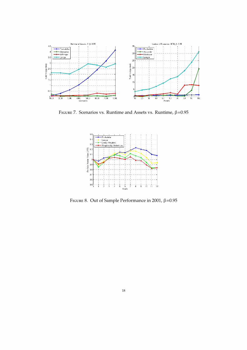
Figure 7. Scenarios vs. Runtime and Assets vs. Runtime, β=0.95

Figure 8. Out of Sample Performance in 2001, β=0.95

18



19

Figure 11. S&P 500, Reference: Google Finance

20

making money with cvar 1. introduction markowitz introduced

Documents