making waves in vector calculus - c.ymcdn.com · areyousittingintherightroom?...

Making Waves in Vector Calculus

<http://blogs.ams.org/blogonmathblogs/2013/04/22/the-mathematics-of-planet-earth/>

J. B. ThooYuba College

2013 AMATYC Conference, Anaheim, California

October 30, 2013

<http://blogs.ams.org/blogonmathblogs/2013/04/22/the-mathematics-of-planet-earth/>

This presentation was produced using LATEX with C. Campani’sBeamer LATEX class and saved as a PDF file:<http://bitbucket.org/rivanvx/beamer>.

See Norm Matloff’s web page<http://heather.cs.ucdavis.edu/~matloff/beamer.html>for a quick tutorial.

Disclaimer: Our slides here won’t show off what Beamer can do.Sorry. :-)

<http://bitbucket.org/rivanvx/beamer>

<http://heather.cs.ucdavis.edu/~matloff/beamer.html>

Are you sitting in the right room?

A common exercise in calculus textbooks is to verify that a givenfunction u = u(x , t) satisfies the heat equation, ut = Duxx , or thewave equation, utt = c2uxx . While this is a useful exercise in usingthe chain rule, it is not a very exciting one because it ends there.

The mathematical theory of waves is a rich source of partialdifferential equations. This talk is about introducing somemathematics of waves to vector calculus students. We will showyou some examples that we have presented to our vector calculusstudents that have given a context for what they are learning.

Outline of the talk

Some examples of waves

Mathematical definition of a wave

Some wave equations

Using what we have learnt

Chain ruleIntegrating factorPartial fractions

Other examples

References

Adrian Constantin, Nonlinear Water Waves with Applications to Wave-CurrentInteractions and Tsunamis, CBMS-NSF Regional Conference Series in AppliedMathematics, Volume 81, Society for Industrial and Applied Mathematics,Philadelphia (2011).

Roger Knobel, An Introduction to the Mathematical Theory of Waves, StudentMathematics Library, IAS/Park City Mathematical Subseries, Volume 3,American Mathematical Society, Providence (2000).

James Lighthill, Waves in Fluids, Cambridge Mathematical Library, CambridgeUniversity Press, Cambridge (1978).

Bruce R. Sutherland, Internal Gravity Waves, Cambridge University Press,Cambridge (2010).

G. B. Whitham, Linear and Nonlinear Waves, A Wiley-Interscience Publication,John Wiley & Sons, Inc., New York (1999)

Some examples of waves

Typical

Pond Guitar Strings

(L) <http://astrobob.areavoices.com/2008/10/12/the-silence-of-crashing-waves/>

(R) <http://rekkerd.org/cinematique-instruments-releases-guitar-harmonics-for-kontakt/>

<http://astrobob.areavoices.com/2008/10/12/the-silence-of-crashing-waves/>

<http://rekkerd.org/cinematique-instruments-releases-guitar-harmonics-for-kontakt/>

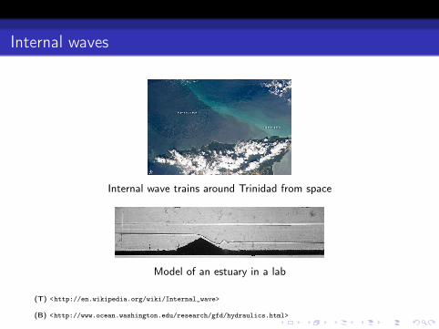
Internal waves

Internal wave trains around Trinidad from space

Model of an estuary in a lab

(T) <http://en.wikipedia.org/wiki/Internal_wave>

(B) <http://www.ocean.washington.edu/research/gfd/hydraulics.html>

<http://en.wikipedia.org/wiki/Internal_wave>

<http://www.ocean.washington.edu/research/gfd/hydraulics.html>

Internal waves

Kelvin-Helmholtz instability

Clouds In a tank

(L) <http://www.documentingreality.com/forum/f241/amazing-clouds-89929/>

(R) <http://www.nwra.com/products/labservices/#tiltingtank>

<http://www.documentingreality.com/forum/f241/amazing-clouds-89929/>

<http://www.nwra.com/products/labservices/#tiltingtank>

Water gravity waves

Deep-water waves

Bow waves or ship waves

(L) <http://wanderinweeta.blogspot.com/2011/12/bow-wave.html>

(R) <http://www.fluids.eng.vt.edu/msc/gallery/waves/jfkkub.jpg>

<http://wanderinweeta.blogspot.com/2011/12/bow-wave.html>

<http://www.fluids.eng.vt.edu/msc/gallery/waves/jfkkub.jpg>

Water gravity waves

Shallow-water waves

Tsunami (2011 Tohoku, Japan, earthquake)

Iwanuma, Japan Crescent City, Ca Santa Cruz, Ca

(L) <http://www.telegraph.co.uk/news/picturegalleries/worldnews/8385237/Japan-disaster-30-powerful-images-of-the-earthquake-and-tsunami.html>

(C) <http://www.katu.com/news/local/117824673.html?tab=gallery&c=y&img=3>

(R) <http://www.conservation.ca.gov/cgs/geologic_hazards/Tsunami/Inundation_Maps/Pages/2011_tohoku.aspx>

<http://www.telegraph.co.uk/news/picturegalleries/worldnews/8385237/Japan-disaster-30-powerful-images-of-the-earthquake-and-tsunami.html>

<http://www.telegraph.co.uk/news/picturegalleries/worldnews/8385237/Japan-disaster-30-powerful-images-of-the-earthquake-and-tsunami.html>

<http://www.katu.com/news/local/117824673.html?tab=gallery&c=y&img=3>

<http://www.conservation.ca.gov/cgs/geologic_hazards/Tsunami/

Inundation_Maps/Pages/2011_tohoku.aspx>

Solitary waves

Morning glory cloud Ocean wave

(L) <http://www.dropbears.com/m/morning_glory/rollclouds.htm>

(R) <http://www.math.upatras.gr/~weele/weelerecentresearch_SolitaryWaterWaves.htm>

<http://www.dropbears.com/m/morning_glory/rollclouds.htm>

<http://www.math.upatras.gr/~weele/weelerecentresearch_SolitaryWaterWaves.htm>

Solitary waves

“I was observing the motion of a boat which was rapidly drawnalong a narrow channel by a pair of horses, when the boat suddenlystopped – not so that mass of water in the channel which it had putin motion; it accumulated round the prow of the vessel in a state ofviolent agitation, then suddenly leaving it behind, rolled forwardwith great velocity, assuming the form of a large solitary elevation, arounded smooth and well-defined heap of water which continued itscourse along the channel apparently without change of form ordiminution of speed. I followed it on horseback, and overtook it stillrolling on at a rate of some eight or nine miles an hour, preservingits original figure some thirty feet long and a foot to a foot and ahalf in height. Its height gradually diminished, and after a chase ofone or two miles I lost it in the windings of the channel.”

J.S. Russell, 1844*

John Scott Russell, Report on waves, Report of the 14th Meeting of the British Association for the

Advancement of Science, 1844, pp. 311–390

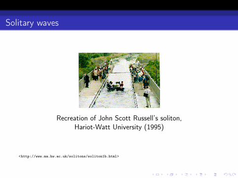
Solitary waves

Recreation of John Scott Russell’s soliton,Hariot-Watt University (1995)

<http://www.ma.hw.ac.uk/solitons/soliton1b.html>

<http://www.ma.hw.ac.uk/solitons/soliton1b.html>

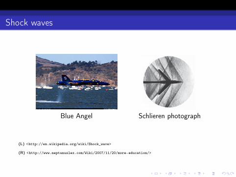
Shock waves

Blue Angel Schlieren photograph

(L) <http://en.wikipedia.org/wiki/Shock_wave>

(R) <http://www.neptunuslex.com/Wiki/2007/11/20/more-education/>

<http://en.wikipedia.org/wiki/Shock_wave>

<http://www.neptunuslex.com/Wiki/2007/11/20/more-education/>

Mathematical definition of a wave

Definition

No single precise definition of what exactly constitutes a wave.Various restrictive definitions can be given, but to cover the wholerange of wave phenomena it seems preferable to be guided by theintuitive view that a wave is any recognizable signal that istransferred from one part of the medium to another with arecognizable velocity of propagation.

[Whitham]

Some wave equations

The wave equation

The wave equation: utt = c2uxx

Models a number of wavephenomena, e.g., vibrations ofa stretched string

Standing wave solution:

un(x , t) = [A cos(nπct/L) + B sin(nπct/L)] sin(nπx/L)

0 L

n = 3, A = B = 0.1, c = L = 1, t = 0 : 0.1 : 1, 0 ≤ x ≤ 1

The Korteweg-de Vries (KdV) equation

The Korteweg-de Vries (KdV) equation: ut + uux + uxxx = 0

Models shallow water gravitywaves

x

u

speed c

Look for traveling wave solution u(x , t) = f (x − ct),

c > 0, f (z), f ′(z), f ′′(z)→ 0 as z → ±∞.

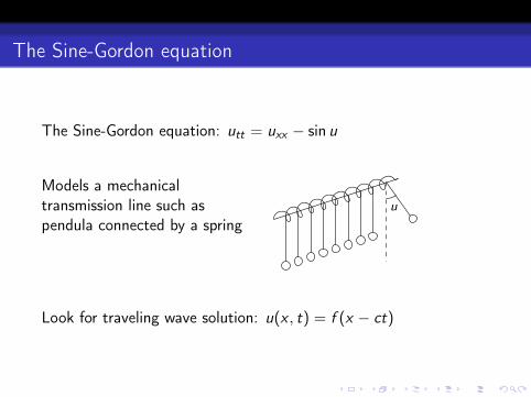
The Sine-Gordon equation

The Sine-Gordon equation: utt = uxx − sin u

Models a mechanicaltransmission line such aspendula connected by a spring

u

Look for traveling wave solution: u(x , t) = f (x − ct)

Using what we have learnt

Chain rule

h = g ◦ f =⇒ Dh = Dg Df

Note: Dg is an m × p matrix if g : Rp → Rm, and Df is a p × nmatrix if f : Rn → Rp

; in this case, h : Rn → Rm and Dh is anm × n matrix

E.g., g : R2 → R : g(x , y) = z , f : R → R2 : f (t) = (x , y), and

h = g ◦ f : R → R : h(t) = z

Dh =[

∂z∂x

∂z∂y

]Dg

[dxdt

dydt

]Df

=⇒ dz

dt=∂z

∂x

dx

dt+∂z

∂y

dy

dt

Chain rule

h = g ◦ f =⇒ Dh = Dg Df

Note: Dg is an m × p matrix if g : Rp → Rm, and Df is a p × nmatrix if f : Rn → Rp; in this case, h : Rn → Rm and Dh is anm × n matrix

E.g., g : R2 → R : g(x , y) = z , f : R → R2 : f (t) = (x , y), and

h = g ◦ f : R → R : h(t) = z

Dh =[

∂z∂x

∂z∂y

]Dg

[dxdt

dydt

]Df

=⇒ dz

dt=∂z

∂x

dx

dt+∂z

∂y

dy

dt

Example 1

The wave equation:* utt = auxx , a > 0


i.e., look for a solution that advects at wave speed c withoutchanging its profile

E.g.,

u(x , t) = sin(x − ct),

u(x , t) = (x − ct)4,

u(x , t) = exp[−(x − ct)2

]*Models a number of wave phenomena, e.g., vibrations of a stretched string

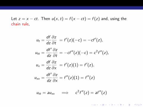
Let z = x − ct. Then u(x , t) = f (x − ct) = f (z) and, using thechain rule,

ut =df

dz

∂z

∂t= f ′(z)(−c) = −cf ′(z),

utt =df ′

dz

∂z

∂t= −cf ′′(z)(−c) = c2f ′′(z),

ux =df

dz

∂z

∂x= f ′(z)(1) = f ′(z),

uxx =df ′

dz

∂z

∂x= f ′′(z)(1) = f ′′(z)

utt = auxx =⇒ c2f ′′(z) = af ′′(z)

c2f ′′(z) = af ′′(z) =⇒ (c2 − a)f ′′(z) = 0

c2 − a = 0 =⇒ c = ±√

a:

u(x , t) = f (x ±√

at) provided f ′′ exists

e.g., u(x , t) = exp[−(x −

√at)2

]f ′′(z) = 0 =⇒ f (z) = A + Bz :

u(x , t) = A + B(x − ct) provided solution is not constant

c2f ′′(z) = af ′′(z) =⇒ (c2 − a)f ′′(z) = 0

c2 − a = 0 =⇒ c = ±√

a:

u(x , t) = f (x ±√


e.g., u(x , t) = exp[−(x −

√at)2

]

f ′′(z) = 0 =⇒ f (z) = A + Bz :


c2f ′′(z) = af ′′(z) =⇒ (c2 − a)f ′′(z) = 0

c2 − a = 0 =⇒ c = ±√

a:

u(x , t) = f (x ±√


e.g., u(x , t) = exp[−(x −

√at)2

]f ′′(z) = 0 =⇒ f (z) = A + Bz :


Example 2

The linearized KdV* equation: ut + ux + uxxx = 0

Look for wave train solution: u(x , t) = A cos(kx − ωt), A 6= 0,

where k > 0, ω > 0

(a particular type of traveling wave solution)

Note: u(x , t) = A cos(k(x − (ω/k)t

)advects at wave speed

c = ω/k

The number ω is the angular frequency and k is called thewavenumber. The wavelength is 2π/k .

*KdV = Korteweg-de Vries; the KdV equation models shallow-water gravitywaves

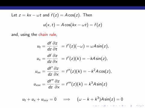
Let z = kx − ωt and f (z) = A cos(z). Then

u(x , t) = A cos(kx − ωt) = f (z)

and, using the chain rule,

ut =df

dz

∂z

∂t= f ′(z)(−ω) = ωA sin(z),

ux =df

dz

∂z

∂x= f ′(z)(k) = −kA sin(z),

uxx =df ′

dz

∂z

∂x= f ′′(z)(k) = −k2A cos(z),

uxxx =df ′′

dz

∂z

∂x= f ′′′(z)(k) = k3A sin(z)

ut + ux + uxxx = 0 =⇒ (ω − k + k3)A sin(z) = 0

(ω − k + k3)A sin(z) = 0 =⇒ ω − k + k3 = 0

Dispersion relation: ω = k − k3

Wave speed: c =ω

k= 1− k2

Note: That c depends on k means that wave trains of differentfrequencies travel at different speeds. Such a wave is called adispersive wave. Here, smaller k or longer waves (λ = 2π/k) speedahead, while larger k or shorter waves trail behind.

Group velocity: C = dωdk = 1− 3k2

The group velocity C is the velocity of the energy in the wave andis generally different from the wave speed c

In general, a wave train solution is u(x , t) = f (kx − ωt),

where k > 0, ω > 0, and f is periodic

(a particular type of traveling wave solution)

In general, not a solution for every possible k or ω

Note: u(x , t) = f(k(x − (ω/k)t

)advects at wave speed c = ω/k

Integrating factor

To solve: y ′(x) + p(x)y(x) = q(x) for y = y(x)

Multiply through by integrating factor µ = µ(x)

µy ′ + µpy = µq

If µ′ = µp, then µy ′ + µpy = µy ′ + µ′y , so that

(µy)′ = µq =⇒ µy =

∫µq dx

and hence

y(x) =1

µ(x)

∫µ(x)q(x) dx where µ(x) = exp

[∫p(x) dx

]

Example

The Sine-Gordon equation: utt = uxx − sin u

Models a mechanicaltransmission line such aspendula connected by a spring

u


Let z = x − ct. Then u(x , t) = f (x − ct) = f (z) and

utt = uxx − sin u =⇒ c2f ′′(z) = f ′′(z)− sin f

To solve the equation in f , we multiply through by f ′(z), anintegrating factor

c2f ′f ′′ = f ′f ′′ − f ′ sin f =⇒ c2(12 f ′ 2

)′=(1

2 f ′ 2)′+ (cos f )′

Now integrate w.r.t. z

12c2f ′ 2 = 1

2 f ′ 2 + cos f + a

To determine a, impose the conditions

f (z), f ′(z)→ 0 as z →∞

i.e., pendula ahead of the wave are undisturbed

Then, as z →∞,

12c2f ′ 2 = 1

2 f ′ 2 + cos f + a → 0 = 0+ cos 0+ a

so that a = −1,

i.e.

12c2f ′ 2 = 1

2 f ′ 2 + cos f − 1 =⇒ f ′ 2 =2

1− c2 (1− cos f )

Exercise:

1 Show that f (z) = 4 arctan[exp(− z√

1− c2

)]is a solution

2 Solve the equation to obtain the solution above(hint: 1− cos f = 2 sin2(f /2))

Then, as z →∞,

12c2f ′ 2 = 1

2 f ′ 2 + cos f + a → 0 = 0+ cos 0+ a

so that a = −1, i.e.

12c2f ′ 2 = 1

2 f ′ 2 + cos f − 1 =⇒ f ′ 2 =2

1− c2 (1− cos f )

Exercise:

1 Show that f (z) = 4 arctan[exp(− z√

1− c2

)]is a solution

2 Solve the equation to obtain the solution above(hint: 1− cos f = 2 sin2(f /2))

Wave front solution:

u(x , t) = 4 arctan[exp(− x − ct√

1− c2

)]

x

u

2π

speed cu

A wave front is a solution u(x , t) for which

limx→−∞

u(x , t) = k1 and limx→∞

u(x , t) = k2

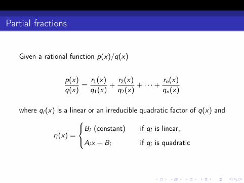
Partial fractions

Given a rational function p(x)/q(x)

p(x)

q(x)=

r1(x)

q1(x)+

r2(x)

q2(x)+ · · ·+ rn(x)

qn(x)

where qi (x) is a linear or an irreducible quadratic factor of q(x) and

ri (x) =

Bi (constant) if qi is linear,

Aix + Bi if qi is quadratic

Example

The KdV equation: ut + uux + uxxx = 0

Look for traveling wave solution that is a pulse:

u(x , t) = f (x − ct),

f (z), f ′(z), f ′′(z)→ 0 as z →∞, where z = x − ct

x

u

speed c

Then

ut + uux + uxxx = 0 =⇒ −cf ′ + ff ′ + f ′′′ = 0

Rewrite,

then integrate

−cf ′ +(1

2 f 2)′ + (f ′′)′ = 0

=⇒ −cf + 12 f 2 + f ′′ = a

To determine a, impose f (z), f ′′(z)→ 0 as z →∞. Then

−cf + 12 f 2 + f ′′ = a → 0+ 0+ 0 = a

so that−cf + 1

2 f 2 + f ′′ = 0

Then

ut + uux + uxxx = 0 =⇒ −cf ′ + ff ′ + f ′′′ = 0

Rewrite, then integrate

−cf ′ +(1

2 f 2)′ + (f ′′)′ = 0 =⇒ −cf + 12 f 2 + f ′′ = a


−cf + 12 f 2 + f ′′ = a → 0+ 0+ 0 = a

so that−cf + 1

2 f 2 + f ′′ = 0

Then

ut + uux + uxxx = 0 =⇒ −cf ′ + ff ′ + f ′′′ = 0


−cf ′ +(1

2 f 2)′ + (f ′′)′ = 0 =⇒ −cf + 12 f 2 + f ′′ = a

To determine a, impose f (z), f ′′(z)→ 0 as z →∞.

Then

−cf + 12 f 2 + f ′′ = a → 0+ 0+ 0 = a

so that−cf + 1

2 f 2 + f ′′ = 0

Then

ut + uux + uxxx = 0 =⇒ −cf ′ + ff ′ + f ′′′ = 0


−cf ′ +(1

2 f 2)′ + (f ′′)′ = 0 =⇒ −cf + 12 f 2 + f ′′ = a


−cf + 12 f 2 + f ′′ = a → 0+ 0+ 0 = a

so that−cf + 1

2 f 2 + f ′′ = 0

Now multiply through by integrating factor f ′, then integrate

− cff ′ + 12 f 2f ′ + f ′f ′′ = 0

=⇒ −c(1

2 f 2)′ + 12

(13 f 3)′ + (1

2 f ′ 2)′= 0

=⇒ −12cf 2 + 1

6 f 3 + 12 f ′ 2 = b

To determine b, impose f (z), f ′(z)→ 0 as z →∞.

Then

−12cf 2 + 1

6 f 3 + 12 f ′ 2 = b → 0+ 0+ 0 = b

so that−1

2cf 2 + 16 f 3 + 1

2 f ′ 2 = 0

Now multiply through by integrating factor f ′, then integrate

− cff ′ + 12 f 2f ′ + f ′f ′′ = 0

=⇒ −c(1

2 f 2)′ + 12

(13 f 3)′ + (1

2 f ′ 2)′= 0

=⇒ −12cf 2 + 1

6 f 3 + 12 f ′ 2 = b

To determine b, impose f (z), f ′(z)→ 0 as z →∞. Then

−12cf 2 + 1

6 f 3 + 12 f ′ 2 = b → 0+ 0+ 0 = b

so that−1

2cf 2 + 16 f 3 + 1

2 f ′ 2 = 0

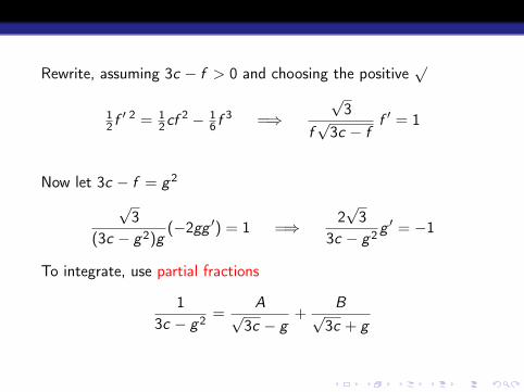
Rewrite, assuming 3c − f > 0 and choosing the positive√

12 f ′ 2 = 1

2cf 2 − 16 f 3 =⇒

√3

f√3c − f

f ′ = 1

Now let 3c − f = g2

√3

(3c − g2)g(−2gg ′) = 1 =⇒ 2

√3

3c − g2 g ′ = −1

To integrate, use partial fractions

13c − g2 =

A√3c − g

+B√

3c + g

13c − g2 =

A√3c − g

+B√

3c + g

=⇒ 1 = A(√3c + g) + B(

√3c − g)

=⇒ A =1

2√3c, B =

12√3c

=⇒ 13c − g2 =

1/2√3c√

3c − g+

1/2√3c√

3c + g

=⇒ 2√3

3c − g2 g ′ =g ′

√c(√3c − g)

+g ′

√c(√3c + g)

2√3

3c − g2 g ′ = −1

=⇒ g ′√

c(√3c − g)

+g ′

√c(√3c + g)

= −1

=⇒ g ′√3c − g

+g ′√

3c + g= −√

c

=⇒ − ln(√3c − g) + ln(

√3c + g) = −

√cz + d

=⇒ ln√3c + g√3c − g

= −√

cz + d

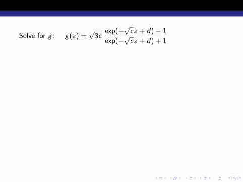
Solve for g : g(z) =√3c

exp(−√

cz + d)− 1exp(−

√cz + d) + 1

Use: tanh ζ =sinh ζcosh ζ

=12(e

ζ − e−ζ)12(e

ζ + e−ζ)= −exp(−2ζ)− 1

exp(−2ζ) + 1

Substitute −2ζ = −√

cz + d :

g(z) = −√3c tanh

[12(√

cz − d)]

Recall f = 3c − g2 and choose d = 0:

f (z) = 3c sech2[12√

cz]

=⇒ u(x , t) = 3c sech2[√

c

2(x − ct)

]

x

u

amplitude 3c

speed c

Soliton solution: u(x , t) = 3c sech2[√

c

2(x − ct)

]

Note: That amplitude is 3c means that taller waves move fasterthan shorter waves.

Other examples

Water gravity waves

Ship waves

Tsunamis

Shock waves

Water gravity waves

Consider water (inviscid incompressible fluid) in a constantgravitational field

Spatial coordinates (x , y , z), fluid velocity ~u = (u, v ,w)

Sinusoidal wave train solution:

η = Ae i(~k·~x−ωt)

water surface, φ = Z (z)e i(~k·~x−ωt)

velocity potential

where the wave oscillates in ~x = (x , y) and t, but not in z ; here ~kis the wavenumber vector and ω is the frequency

Dispersion relation: ω2 = gk tanh(kd) , k = |~k | = 2π/λ

Water gravity waves






velocity potential

where the wave oscillates in ~x = (x , y) and t, but not in z

; here ~kis the wavenumber vector and ω is the frequency


Water gravity waves






velocity potential



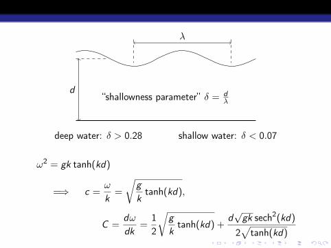
d

λ

“shallowness parameter” δ = dλ

deep water: δ > 0.28 shallow water: δ < 0.07

ω2 = gk tanh(kd)

=⇒ c =ω

k=

√g

ktanh(kd),

C =dω

dk=

12

√g

ktanh(kd) +

d√

gk sech2(kd)

2√

tanh(kd)

Deep water: δ →∞ at fixed k

Using limθ→∞

tanh(θ) = 1

c =ω

k=

√g

ktanh(2πδ) →

√g

k

C =dω

dk=

12

√g

ktanh(2πδ) +

d√

gk sech2(2πδ)2√

tanh(2πδ)

→ 12

√g

k=

12

c

Energy in the wave propagates at half the wave speed

travels at wave speed c = ω/k

travels at group velocity C = dω/dk

Ship waves

Shallow water: δ → 0 at fixed d

Using limθ→0

tanh(θ)θ

= 1

c =ω

k=

√gd

tanh(2πδ)2πδ

→√

gd

C =dω

dk=

12

√gd

tanh(2πδ)2πδ

+d√

g · 2πδ/d sech2(2πδ)2√

tanh(2πδ)

→ 12

√gd +

d

2

√g

d=√

gd

Energy in the wave propagates at the wave speed

Tsunamis

Typical wavelength of several hundred kilometers and deepest pointin the ocean in the Marianas Trench (Western Pacific Ocean) about11 kilometers makes a tsunami a shallow-water wave (long wave)

Wave speed c =√

gd

E.g., ocean depth 4 kilometers, gravity 9.8 m/s2 yields a wavespeed c =

√39 200 m/s ≈ 200 m/s or about 445 mph

Typical amplitude in the open ocean about 1 m, but rises up to10 m to 15 m as approaches shore

d d

λ

a

Energy in the wave proportional to a2c ≈ a2√gd remains constant, so a

increases as d decreases

Hat Ray Leach beach, Thailand, December 2004

<http://geol105naturalhazards.voices.wooster.edu/page/32/>

<http://geol105naturalhazards.voices.wooster.edu/page/32/>

Obtaining the dispersion relation



Equations

ρ

(∂~u

∂t+ (~u ·∇)~u

)= −∇p − ρg(0, 0, 1),

∇ · ~u = 0

Assume irrotational ∇× ~u = 0 and let φ be velocity potential

Let z = η(x , y , t) describe water surface

For small perturbation on water initially at rest, depth −d0, thelinearized equations are

φxx + φyy + φzz = 0, − d0 < y < 0,

φtt + gφz = 0, y = 0,

φz + d0xφx + d0yφy = 0, y = −d0

After solving for φ, find surface

η(x , y , t) = − 1gφt(x , y , 0, t)


η = Ae i(~k·~x−ωt), φ = Z (z)e i(~k·~x−ωt)


Substitute into the linearized equations

Dispersion relation: ω2 = gk tanh(kd0), k = |~k|

Shock waves

Length of “wire” occupying interval [a, b] on the real line, and Qthe amount of “stuff” in [a, b]

xa b

u(x , t) =Q

length= density of Q,

φ(x , t) =Q

time= flux function for Q,

f (x , t) =Q

time · length= source function for Q

Conservation law:

d

dt

∫ b

au(x , t) dx = φ(a, t)− φ(b, t) +

∫ b

af (x , t) dx

time rate of change of mass = amount entering left end

− amount leaving right end

+ amount added by source

If u, φ, and f have continuous first derivatives, then

ut + φx = f

In general, φ depends on u: ut + φuux = f

Example 1

Advection equation: φ(u) = cu, c constant, f = 0

ut + cux = 0,

u(x , 0) = u0(x), x ∈ (−∞,∞), t ∈ [0,∞)

Suppose x = x(t). Then u(x , t) = u(x(t), t), so by the chain rule

du

dt=∂u

∂x

dx

dt+∂u

∂t

If dx/dt = c , then

ut + cux = 0 =⇒ du

dt= 0,

so that u is constant on characteristic curves defined by dx/dt = c

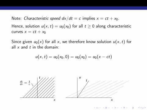
Note: Characteristic speed dx/dt = c implies x = ct + x0.

Hence, solution u(x , t) = u0(x0) for all t ≥ 0 along characteristiccurves x = ct + x0

Since given u0(x) for all x , we therefore know solution u(x , t) forall x and t in the domain:

u(x , t) = u0(x0, 0) = u0(x0) = u0(x − ct)

t

x

dtdx

= 1c

u

x

t

Note: Charcteristic speed dx/dt = c implies x = ct + x0.

Hence, solution u(x , t) = u0(x0) for all t ≥ 0 along characteristiccurves x = ct + x0

Since given u0(x) for all x , we therefore know solution u(x , t) forall x and t in the domain:

u(x , t) = u0(x0, 0) = u0(x0) = u0(x − ct)

t

x

dtdx

= 1c

u

x

t

Example 2

Inviscid Burgers equation: φ(u) = 12u2, f = 0

ut + uux = 0,

u(x , 0) = u0(x), x ∈ (−∞,∞), t ∈ [0,∞)

Again, suppose x = x(t), so that dudt = ∂u

∂xdxdt +

∂u∂t . Then

ut + uux = 0

=⇒ du

dt= 0 along

dx

dt= u(x(t), t), x(0) = x0

Note: Characteristic speed dx/dt = u, not constant

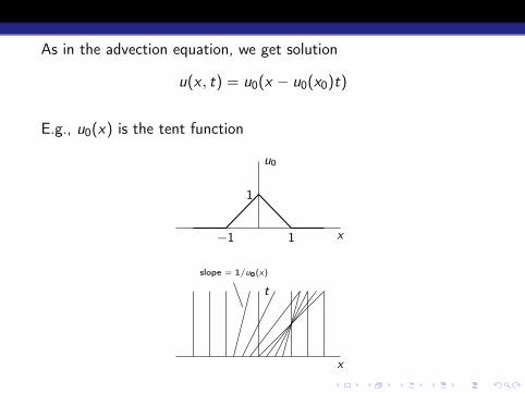
As in the advection equation, we get solution

u(x , t) = u0(x − u0(x0)t)

E.g., u0(x) is the tent function

x

u0

−1 1

1

x

t

slope = 1/u0(x)

Time series

x

u

−1 1

1

x

u

−1 1

1

x

u

−1 1

1

x

u

−1 1

1shock forms

x

u

−1 1

1no longer a function

x

u

−1 1

1

To define solution beyond shock formation: equal area rule

x

u

−1 1

1shock forms

x

u

−1 1

1shock propogates

x

u

−1 1

1

x

u

−1 1

1

Note: The amplitude diminishes as the shock propogates

More

Can find time when shock forms (breaking time)

Can find the shock speed

But that would have to wait for another day.

References

Adrian Constantin, Nonlinear Water Waves with Applications to Wave-CurrentInteractions and Tsunamis, CBMS-NSF Regional Conference Series in AppliedMathematics, Volume 81, Society for Industrial and Applied Mathematics,Philadelphia (2011).

Roger Knobel, An Introduction to the Mathematical Theory of Waves, StudentMathematics Library, IAS/Park City Mathematical Subseries, Volume 3,American Mathematical Society, Providence (2000).

James Lighthill, Waves in Fluids, Cambridge Mathematical Library, CambridgeUniversity Press, Cambridge (1978).

Bruce R. Sutherland, Internal Gravity Waves, Cambridge University Press,Cambridge (2010).

G. B. Whitham, Linear and Nonlinear Waves, A Wiley-Interscience Publication,John Wiley & Sons, Inc., New York (1999)

making waves in vector calculus - c.ymcdn.com · areyousittingintherightroom?...

Documents