mallee pwa – murrayville wspa groundwater model€¦ · mallee pwa – murrayville wspa...
TRANSCRIPT

DWLBC REPORT
Mallee PWA - Murrayville
WSPA Groundwater Model
2006/27

Mallee PWA – Murrayville WSPA Groundwater Model
Steve Barnett and Kwadwo Osei-bonsu
Knowledge and Information Division Department of Water, Land and Biodiversity Conservation
December 2006
Report DWLBC 2006/27
Knowledge and information Division Department of Water, Land and Biodiversity Conservation 25 Grenfell Street, Adelaide GPO Box 2834, Adelaide SA 5001 Telephone National (08) 8463 6946 International +61 8 8463 6946 Fax National (08) 8463 6999 International +61 8 8463 6999 Website www.dwlbc.sa.gov.au Disclaimer The Department of Water, Land and Biodiversity Conservation and its employees do not warrant or make any representation regarding the use, or results of the use, of the information contained herein as regards to its correctness, accuracy, reliability, currency or otherwise. The Department of Water, Land and Biodiversity Conservation and its employees expressly disclaims all liability or responsibility to any person using the information or advice. Information contained in this document is correct at the time of writing. © Government of South Australia, through the Department of Water, Land and Biodiversity Conservation 2006 This work is Copyright. Apart from any use permitted under the Copyright Act 1968 (Cwlth), no part may be reproduced by any process without prior written permission obtained from the Department of Water, Land and Biodiversity Conservation. Requests and enquiries concerning reproduction and rights should be directed to the Chief Executive, Department of Water, Land and Biodiversity Conservation, GPO Box 2834, Adelaide SA 5001. ISBN-13 978-1-921218-28-6 Preferred way to cite this publication Barnett, S.R. and Osei-bonsu, K., 2006. Mallee PWA – Murrayville WSPA Groundwater Model. South Australia. Department of Water, Land and Biodiversity Conservation. DWLBC Report 2006/27.

Report DWLBC 2006/27 Mallee PWA – Murrayville WSPA Groundwater Model
iii
FOREWORD
South Australia’s unique and precious natural resources are fundamental to the economic and social wellbeing of the State. It is critical that these resources are managed in a sustainable manner to safeguard them both for current users and for future generations.
The Department of Water, Land and Biodiversity Conservation (DWLBC) strives to ensure that our natural resources are managed so that they are available for all users, including the environment.
In order for us to best manage these natural resources it is imperative that we have a sound knowledge of their condition and how they are likely to respond to management changes. DWLBC scientific and technical staff continues to improve this knowledge through undertaking investigations, technical reviews and resource modelling.
Rob Freeman CHIEF EXECUTIVE DEPARTMENT OF WATER, LAND AND BIODIVERSITY CONSERVATION

Report DWLBC 2006/27 Mallee PWA – Murrayville WSPA Groundwater Model
iv
Report DWLBC 2006/27 Mallee PWA – Murrayville WSPA Groundwater Model
v
CONTENTS
FOREWORD........................................................................................................................... iii
1. INTRODUCTION...............................................................................................................1
2. PREVIOUS MODELLING .................................................................................................2
3. HYDROGEOLOGY ...........................................................................................................3
3.1 REGIONAL HYDROGEOLOGY.................................................................................3 3.2 RECHARGE ...............................................................................................................6
4. MODEL CONSTRUCTION ...............................................................................................7
4.1 EXTENT .....................................................................................................................7 4.2 STRATIGRAPHY .......................................................................................................7 4.3 BOUNDARY CONDITIONS .....................................................................................10 4.4 STARTING HEADS..................................................................................................12 4.5 AQUIFER PARAMETERS........................................................................................12 4.6 RECHARGE .............................................................................................................13 4.7 PUMPING DATA ......................................................................................................13
5. MODEL CALIBRATION..................................................................................................15
5.1 STEADY-STATE MODEL CALIBRATION................................................................15 5.1.1 Hydraulic Parameters ........................................................................................................21 5.1.2 Steady State Sensitivity Analysis.......................................................................................23 5.1.3 Non-Uniqueness ................................................................................................................25
5.2 TRANSIENT MODEL CALIBRATION ......................................................................25 5.2.1 Hydraulic Parameters ........................................................................................................28 5.2.2 Transient Sensitivity Analysis ............................................................................................31 5.2.3 Non-Uniqueness ................................................................................................................32
6. MODEL LIMITATIONS ...................................................................................................33
7. WATER BALANCE.........................................................................................................35
7.1 DOWNWARD LEAKAGE .........................................................................................36
8. SCENARIO MODELLING...............................................................................................38
8.1 SCENARIO 1............................................................................................................38 8.2 SCENARIO 2............................................................................................................41 8.3 SCENARIO 3............................................................................................................41 8.4 SCENARIO 4............................................................................................................41 8.5 ZONE 11A ................................................................................................................41 8.6 ZONE 10A ................................................................................................................46
CONTENTS
Report DWLBC 2006/27 Mallee PWA – Murrayville WSPA Groundwater Model
vi
8.7 ZONE 10B ................................................................................................................48 8.8 DOWNWARD LEAKAGE .........................................................................................49 8.9 DEPRESSURISATION.............................................................................................50
9. SALINITY MODELLING .................................................................................................52
9.1 BOUNDARY CONDITIONS .....................................................................................52 9.2 INITIAL SALINITY AND INPUT PARAMETERS ......................................................54 9.3 SALINITY MODEL CALIBRATION...........................................................................55 9.4 SALINITY MODEL SENSITIVITY ANALYSIS ..........................................................57 9.5 SALINITY MODEL LIMITATIONS ............................................................................58 9.6 RESULTS.................................................................................................................59
10. SUMMARY......................................................................................................................62
APPENDICES........................................................................................................................64
A. TRANSIENT CALIBRATION RESULTS .......................................................................64 B. SCENARIO PREDICTION RESULTS...........................................................................72 C. SALINITY PREDICTION RESULTS .............................................................................80
GLOSSARY ...........................................................................................................................87
REFERENCES.......................................................................................................................88
CONTENTS
Report DWLBC 2006/27 Mallee PWA – Murrayville WSPA Groundwater Model
vii
TABLES
Table 1. MGL aquifer test results.......................................................................................12 Table 2. Specific yield and specific storage values ...........................................................13 Table 3. Steady state calibration statistics.........................................................................16 Table 4. Statistics of the absolute residuals ......................................................................16 Table 5. Vertical hydraulic gradient between MGL and RG aquifers.................................19 Table 6. Vertical hydraulic gradient between MGL and PS aquifers .................................19 Table 7. Sensitivity analyses of steady state input parameters .........................................23 Table 8. Transient calibration statistics for MGL aquifer (m) .............................................26 Table 9. Average root mean square error for MGL aquifer (m) .........................................31 Table 10. Groundwater budget for MGL aquifer (ML/year)..................................................35 Table 11. Solute transport parameters ................................................................................55
FIGURES
Figure 1. Location of Mallee PWA, Murrayville WSPA and model extent .............................1 Figure 2. Simplified geology of the Murray Basin .................................................................4 Figure 3. Potentiometric surface contours for the MGL aquifer ............................................5 Figure 4. Salinity zones for the MGL aquifer.........................................................................5 Figure 5. Hydrogeological cross section ...............................................................................7 Figure 6. Model grid and points of extraction........................................................................8 Figure 7. Aquifer thicknesses in metres................................................................................9 Figure 8. Model boundary conditions..................................................................................11 Figure 9. Pumping extractions in the model area ...............................................................14 Figure 10. Computed vs observed head steady state calibration results..............................17 Figure 11. Residual vs observed head steady state calibration results ................................18 Figure 12. Comparison of pre-development computed and observed water levels ..............20 Figure 13. Aquitard vertical hydraulic conductivity zones (m/day) ........................................21 Figure 14. Hydraulic conductivity zones for the three aquifers (m/day) ................................22 Figure 15. Sensitivity analyses for MGL and RG aquifers ....................................................24 Figure 16. Transient calibration result for MGL obs well PEB 24 .........................................26 Figure 17. Transient calibration statistics over time..............................................................27 Figure 18. Specific yield values for the PS and MGL aquifers..............................................29 Figure 19. Specific storage values for the MGL and RG aquifers.........................................30 Figure 20. Transient sensitivity analysis for the MGL aquifer ...............................................31 Figure 21. Transient calibration result for PS obs well PEB 3 ..............................................32 Figure 22. Schematic steady state water balance for SA and Victoria (ML/yr) .....................36 Figure 23. Extent of pre-irrigation leakage between the MGL and PS aquifers....................37 Figure 24. Comparison of modelled and observed 2004 drawdown and water levels..........39 Figure 25. Schematic water balance for 2004–05 irrigation season (ML/yr).........................40 Figure 26. Scenario 1 results for 2030..................................................................................42 Figure 27. Scenario 2 results for 2030..................................................................................43 Figure 28. Scenario 3 results for 2030..................................................................................44

CONTENTS
Report DWLBC 2006/27 Mallee PWA – Murrayville WSPA Groundwater Model
viii
Figure 29. Scenario 4 results for 2030..................................................................................45 Figure 30. Typical hydrographs of results for Zone 11A .......................................................46 Figure 31. Typical hydrographs of results for Zone 10A .......................................................47 Figure 32. Typical hydrographs of results for Zone 10B .......................................................48 Figure 33. Extent of modelled leakage between the MGL and PS aquifers in 2030.............49 Figure 34. Example of depressurisation in the Northern Adelaide Plains.............................50 Figure 35. Extent of depressurisation during modelling scenarios........................................51 Figure 36. Salinity model boundary conditions .....................................................................53 Figure 37. Initial model salinity concentrations .....................................................................54 Figure 38. Modelled steady state salinity disribution in PS and MGL aquifers .....................56 Figure 39. Computed vs observed salinity steady state calibration results ..........................57 Figure 40. Salinity model sensitivity analysis for the MGL aquifer ........................................58 Figure 41. Salinity predictions in SA .....................................................................................60 Figure 42. Salinity predictions in Victoria ..............................................................................61 Figure 43. Location of SA representative wells for transient calibration ...............................64 Figure 44. Location of Vic representative wells for transient calibration ...............................69 Figure 45. Location of SA representative wells for scenario predictions ..............................72 Figure 46. Location of Vic representative wells for scenario predictions ..............................76 Figure 47. Location of SA representative wells for salinity predictions .................................80 Figure 48. Location of Vic representative wells for salinity predictions.................................84
Report DWLBC 2006/27 Mallee PWA – Murrayville WSPA Groundwater Model
1
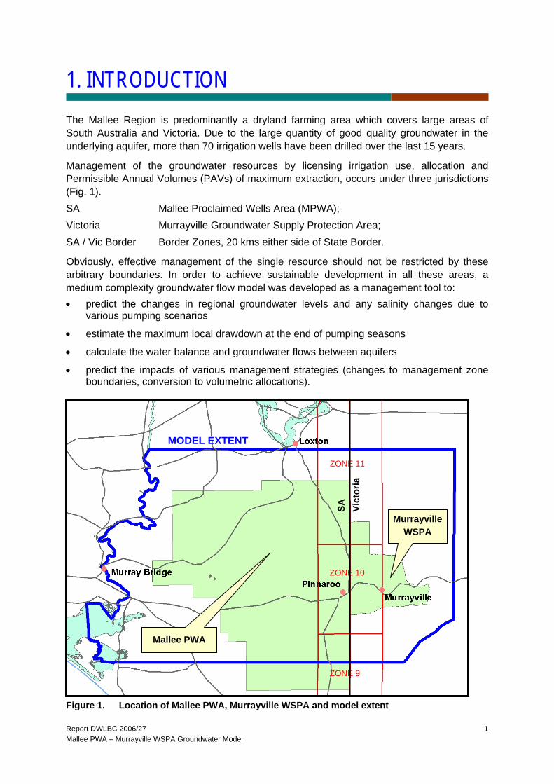
1. INTRODUCTION The Mallee Region is predominantly a dryland farming area which covers large areas of South Australia and Victoria. Due to the large quantity of good quality groundwater in the underlying aquifer, more than 70 irrigation wells have been drilled over the last 15 years.
Management of the groundwater resources by licensing irrigation use, allocation and Permissible Annual Volumes (PAVs) of maximum extraction, occurs under three jurisdictions (Fig. 1). SA Mallee Proclaimed Wells Area (MPWA); Victoria Murrayville Groundwater Supply Protection Area; SA / Vic Border Border Zones, 20 kms either side of State Border.
Obviously, effective management of the single resource should not be restricted by these arbitrary boundaries. In order to achieve sustainable development in all these areas, a medium complexity groundwater flow model was developed as a management tool to: • predict the changes in regional groundwater levels and any salinity changes due to
various pumping scenarios
• estimate the maximum local drawdown at the end of pumping seasons
• calculate the water balance and groundwater flows between aquifers
• predict the impacts of various management strategies (changes to management zone boundaries, conversion to volumetric allocations).
Figure 1. Location of Mallee PWA, Murrayville WSPA and model extent
Murrayville WSPA
Mallee PWA
ZONE 9
ZONE 11
ZONE 10
MODEL EXTENT
SA
Vict
oria
Report DWLBC 2006/27 Mallee PWA – Murrayville WSPA Groundwater Model
2
2. PREVIOUS MODELLING
Two groundwater flow models have previously been developed in the Mallee region to predict trends in groundwater levels. Barnett (1990) constructed a five layer finite element groundwater flow model, covering the whole of the Mallee region of both SA and Victoria. It had a coarse 25 km grid and was used to predict the groundwater level changes caused by increased recharge rates due to the clearing of native vegetation, and assessed the impacts on the salinity of the River Murray.
An improved model was constructed in using the Visual MODFLOW package (Barnett and Yan, 2000), and its subsequent calibration with observed groundwater level data. Improvements include an increase to five layers to take into account inter-aquifer leakage, a more accurate representation of the top surfaces of the various layers, and a much smaller grid size averaging 500 m by 500 m.
This report covers the construction of a new model using the GMS package which covers a larger area to include the expansion of the Mallee PWA and the whole of the Murrayville WSPA.
A glossary of terms is presented toward the end of this report.

Report DWLBC 2006/27 Mallee PWA – Murrayville WSPA Groundwater Model
3
3. HYDROGEOLOGY
A detailed description of the geology and hydrogeology of the region has been presented in several previous publications (Lawrence 1975, Barnett 1983, Brown and Stephenson 1991), as well as the Murray Basin Hydrogeological Map series and numerous reports by the Border Groundwater Review Committee. A summary is presented below.
3.1 REGIONAL HYDROGEOLOGY The Murray Basin extends over 300 000 km2 of inland southeastern Australia and encompasses three States - South Australia, Victoria and New South Wales (Fig. 2). It contains Cainozoic sediments comprising sand, clay and limestone deposited in shallow-marine, fluvio-lacustrine and aeolian environments. These sediments attain a maximum thickness of about 600 m in the Renmark area.
There are three main aquifer systems in the Mallee Region - the Renmark Group confined aquifer, the Murray Group Limestone aquifer and the Pliocene Sands aquifer. Figure 2 shows these aquifers are mainly recharged in the high rainfall areas around the basin margins, with groundwater flowing along extended flowpaths under low gradients before discharging to the River Murray, either by upward leakage from confined aquifers or direct hydraulic connection from the watertable aquifers.
The five main hydrogeological units (aquifers and confining layers) found in the Mallee Region are discussed below in order of increasing depth:
Pliocene Sands aquifer (PS): generally an unconfined aquifer which is saturated mostly in Victoria. The unit comprises unconsolidated to weakly cemented fine to coarse sand and is generally over 50 m in thickness. The groundwater flow is generally towards the north where discharge occurs to the River Murray. Salinity in the aquifer ranges from 1000 mg/L in the south, to over 35 000 mg/L to the north. Because the aquifer is thin and contains saline groundwater, there are no significant extractions.
Bookpurnong Beds (confining layer): this unit is absent over most of the SA Mallee, however it dips down gradually to the east and increases in thickness into Victoria. It commonly occurs as a low permeability unit between the Pliocene Sands aquifer and the underlying limestone aquifer. It comprises poorly consolidated plastic silts, clays and sands up to 30 m in thickness.
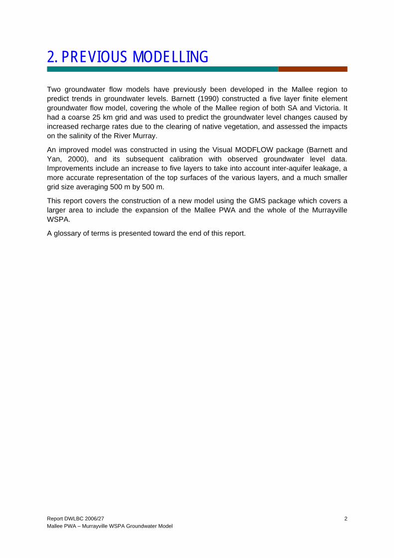
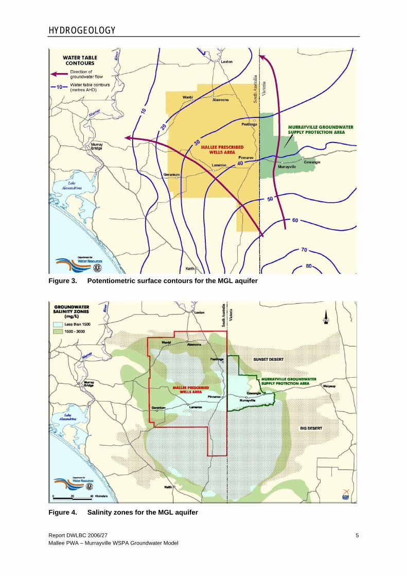
Murray Group Limestone aquifer (MGL): comprises a consolidated, highly fossiliferous, fine to coarse bioclastic limestone which averages 100 m in thickness. Groundwater movement is generally to the north and northwest under low gradients from recharge areas in southwest Victoria. Figure 3 shows the potentiometric surface contours and the direction of groundwater movement in the limestone aquifer. The volume of irrigation quality groundwater in storage in the limestone aquifer is estimated at 100 million ML, with a rate of groundwater movement downgradient of only 0.5 m/yr. Salinities in the aquifer slowly increase downgradient from less than 1000 mg/L in recharge areas, to over 20 000 mg/L where the aquifer discharges to the River Murray. Salinity zones in the Mallee Region are shown in Figure 4.

HYDROGEOLOGY
Report DWLBC 2006/27 Mallee PWA – Murrayville WSPA Groundwater Model
4
Murrumbidgee
River
RIVER
MURRAY
MT
LOFT
YR
AN
GES
ETTRICK FORMATION
A1
A1
A
SOUTH AUSTRALIA VICTORIAMURRAY RIVER
KILOMETRES
0 200
PLIOCENE SANDS
WATERTABLE
PinnarooWanbi
MURRAY GROUP
RENMARK GROUP
Mount GambierOTWAY
BASINGIPPSLAND
BASIN
Horsham
GRAMPIANS
MURRAYBASIN
Pinnaroo
Nhill
Kerang
Horsham
Renmark
VICTORIA
GREAT DIVIDING RANGE
River
NEW SOUTH
WALESSOUTH
AUSTRALIA
Darlin
gKILOMETRES
GREAT ARTESIAN BASIN
0 200
100
S.L.
100
200
300
METRES
A
MURRAY BASIN
Sand and clay
Extent of limestone
River
Lach
lan
Bedrock
Loxton
WanbiADELAIDE
200040
GROUNDWATER FLOW
MELBOURNE
Broken Hill
Lameroo
Figure 2. Simplified geology of the Murray Basin
HYDROGEOLOGY
Report DWLBC 2006/27 Mallee PWA – Murrayville WSPA Groundwater Model
5
Figure 3. Potentiometric surface contours for the MGL aquifer
Figure 4. Salinity zones for the MGL aquifer
HYDROGEOLOGY
Report DWLBC 2006/27 Mallee PWA – Murrayville WSPA Groundwater Model
6
The limestone aquifer is the only aquifer developed in the Mallee and is widely used for stock and domestic, irrigation and town water supply purposes. Fully penetrating irrigation wells average about 180 m in depth below ground level and yield up to 60 L/sec using open hole completions over the limestone interval. The aquifer is confined by the overlying Bookpurnong Beds in the eastern portion of the Mallee.
Ettrick Formation (confining layer): occurs between the Murray Group Limestone and the underlying aquifer. The unit is around 15 m in thickness and comprises a glauconitic and fossiliferous marl.
Renmark Group aquifer (RG): a confined aquifer underlying the Ettrick Formation. The unit comprises unconsolidated carbonaceous sands, silt and clay and averages 150 m in thickness. Groundwater flow is from southeast to the west and northwest, similar to the overlying limestone aquifer. The salinity of the groundwater ranges from 500–3000 mg/L, again in a similar distribution to limestone aquifer. There is no extraction from this aquifer because of its depth (over 200 m), and uncertainty in finding large supplies from the interbedded sands and clays.
3.2 RECHARGE Prior to European settlement, the Mallee region was covered by deep-rooted native vegetation, which has a very high water use from the low 250 mm annual rainfall, allowing a recharge rate from rainfall of less than 1 mm/yr. Significant areas have been cleared since 1920 for shallow-rooted dryland annual crops, which has dramatically increased recharge to over 10 mm/yr.
However, because the aquifer is 50 m below ground surface, the increased recharge rate has yet to percolate down to the aquifer and will not do so for several decades. Consequently, the aquifer is currently experiencing the low pre-clearing rate of less than 1 mm/yr. In fact, the large areas of good quality groundwater were probably recharged beneath areas of deep sand (Big Desert, Ngarkat CP, Billiat CP) about 20 000 years ago during much wetter climatic regimes (Leaney and Herczeg, 1999). These sandy areas are shown as brown shading in Figure 4, and their correlation with low groundwater salinity is quite obvious. The northward movement of this low salinity groundwater over thousands of years beyond the boundary of the deep sand, can be seen in the Pinnaroo and Murrayville areas. In the eastern half of the region where the limestone aquifer is confined, there is no direct recharge from rainfall.
The impending increase in recharge due to clearing of at least an order of magnitude, will far outweigh any changes in recharge due to climate change which may affect rainfall by only 20–25%.
Report DWLBC 2006/27 Mallee PWA – Murrayville WSPA Groundwater Model
7
4. MODEL CONSTRUCTION
GMS is a comprehensive MODFLOW interface that provides tools for every phase of groundwater simulation including site characterisation, model development, post-processing, calibration and visualization. With GMS, models can be defined and edited at conceptual model level or on a cell-by-cell basis at the grid level. In addition to MODFLOW, GMS has interfaces to solute transport and particle tracking models (MODPATH, MT3DMS, RT3D, and VS2D).
MODFLOW is a widely used modular finite-difference model that simulates the flow of groundwater of uniform density (McDonald and Harbaugh, 1988) MODFLOW solves the 3-D partial differential equation of groundwater flow with an implicit finite difference scheme in rectangular coordinates.
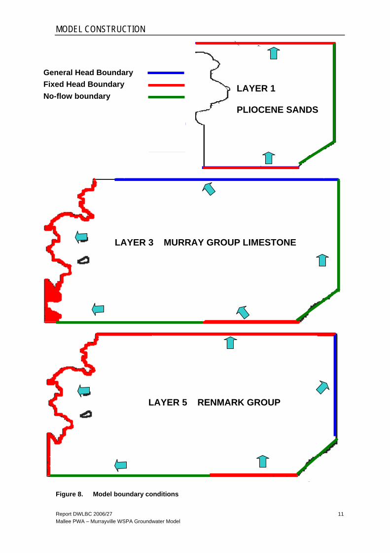
4.1 EXTENT The Mallee region model encompasses an area of about 23 600 km2 and extends 220 km (east to west) by 114 km (north to south). It covers an area from the River Murray in the west, to 64 km into Victoria (E 562 000) in the east, from Ngarkat – Big Desert (N 6054 500) in the south, to N 6167 000 in the north. It has a fine grid size of 170 x 250 m over the central model area (for increased resolution of flow and salinity transport results), increasing to 1200 x 1500 m at the edges of the model. Figure 6 displays the model grid and the points of extraction.
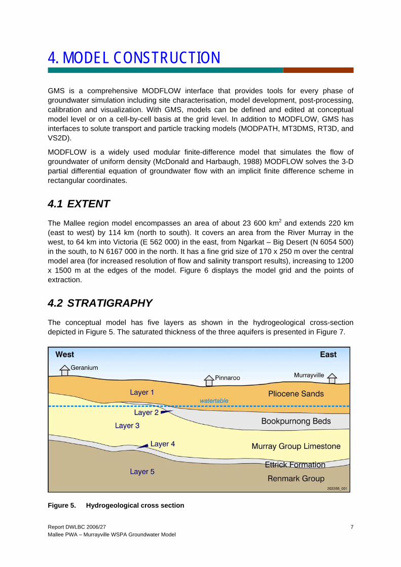
4.2 STRATIGRAPHY The conceptual model has five layers as shown in the hydrogeological cross-section depicted in Figure 5. The saturated thickness of the three aquifers is presented in Figure 7.
Figure 5. Hydrogeological cross section

Figure 6. Model grid and points of extraction
Pinnaroo Lameroo
Murrayville
Karoonda
Wanbi

Report DWLBC 2006/27 Mallee PWA – Murrayville WSPA Groundwater Model
9
Figure 7. Aquifer thicknesses in metres
CONFINED UNCONFINED
PS
MGL
RG
MODEL CONSTRUCTION
Report DWLBC 2006/27 Mallee PWA – Murrayville WSPA Groundwater Model
10
• Layer 1 — Pliocene Sands aquifer (PS); saturated only in eastern third of model area, with groundwater flow to the north. There is no pumping from this layer.
• Layer 2 — Bookpurnong Beds confining layer; absent in western third of model area, controls leakage between PS and MGL aquifers.
• Layer 3 — Murray Group Limestone aquifer (MGL); confined/unconfined aquifer with groundwater flow to the north. All extractions are from this layer.
• Layer 4 — Ettrick Formation confining layer ; covers whole model area, controls leakage between RG and MGL aquifers.
• Layer 5 — Renmark Group confined aquifer (RG); averages 150 m in thickness. There is no pumping from this layer.
The tops of the layers were taken from the Murray Basin hydrogeological map series, but in the Mallee area, the tops of the confining layer (Bookpunong Fm) and MGL aquifer were refined by a reappraisal of geological logs.
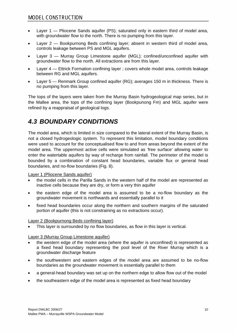
4.3 BOUNDARY CONDITIONS The model area, which is limited in size compared to the lateral extent of the Murray Basin, is not a closed hydrogeologic system. To represent this limitation, model boundary conditions were used to account for the conceptualised flow to and from areas beyond the extent of the model area. The uppermost active cells were simulated as ‘free surface’ allowing water to enter the watertable aquifers by way of recharge from rainfall. The perimeter of the model is bounded by a combination of constant head boundaries, variable flux or general head boundaries, and no-flow boundaries (Fig. 8).
Layer 1 (Pliocene Sands aquifer) • the model cells in the Parilla Sands in the western half of the model are represented as
inactive cells because they are dry, or form a very thin aquifer
• the eastern edge of the model area is assumed to be a no-flow boundary as the groundwater movement is northwards and essentially parallel to it
• fixed head boundaries occur along the northern and southern margins of the saturated portion of aquifer (this is not constraining as no extractions occur).
Layer 2 (Bookpurnong Beds confining layer) • This layer is surrounded by no flow boundaries, as flow in this layer is vertical.
Layer 3 (Murray Group Limestone aquifer) • the western edge of the model area (where the aquifer is unconfined) is represented as
a fixed head boundary representing the pool level of the River Murray which is a groundwater discharge feature
• the southwestern and eastern edges of the model area are assumed to be no-flow boundaries as the groundwater movement is essentially parallel to them
• a general-head boundary was set up on the northern edge to allow flow out of the model
• the southeastern edge of the model area is represented as fixed head boundary
MODEL CONSTRUCTION
Report DWLBC 2006/27 Mallee PWA – Murrayville WSPA Groundwater Model
11
General Head Boundary Fixed Head Boundary No-flow boundary
Figure 8. Model boundary conditions
LAYER 5 RENMARK GROUP
LAYER 1
PLIOCENE SANDS
LAYER 3 MURRAY GROUP LIMESTONE
MODEL CONSTRUCTION
Report DWLBC 2006/27 Mallee PWA – Murrayville WSPA Groundwater Model
12
Layer 4 (Ettrick Formation confining layer) • this layer is surrounded by no flow boundaries as flow in this layer is predominantly
vertical
Layer 5 (Renmark Group confined aquifer) • this layer has a general head boundary along the eastern margin and constant head
boundaries along the northern, western and southeastern margins. This is not constraining, as ther is no pumping from this layer
4.4 STARTING HEADS Starting heads were taken from recent observations from the Murray Group Limestone aquifer, Renmark Group confined aquifer and new observation wells completed in Pliocene Sands. Outside the areas affected by pumping, water levels are mostly constant and unaffected by recharge.
4.5 AQUIFER PARAMETERS Spatially distributed aquifer parameters used in the model include horizontal and vertical hydraulic conductivity, specific yield, specific storage, recharge from rainfall and groundwater extraction from Layer 3. The initial hydraulic conductivity distributions used in the model arrays were derived from the calibrated model of Barnett and Yan (2000), and were based on lithology and the expected range of hydraulic conductivity values determined from aquifer tests carried out on town water supply and irrigation wells that almost fully penetrate the Murray Group Limestone aquifer (Table 1). Because of the limited extent of the Pliocene Sands aquifer, no tests have been carried out in the modelled area, but further to the north in the Noora area, a range of 3–15 m/day was obtained from aquifer tests (Williams, 1976).
Table 1. MGL aquifer test results
Location Hydraulic conductivity (m/day)
Storage coefficient
Pinnaroo 3.3 4.0 x 10⁻⁴
Lameroo 2.2 1.4 x 10⁻²
Parilla 7.2 8.0 x 10⁻⁴
Geranium 7.3 9.6 x 10⁻⁴
Karoonda 0.7
Karte 3.7 2.3 x 10⁻³
Wanbi 2.2 2.5 x 10⁻³
The vertical hydraulic conductivity in the entire model is simulated as a constant factor of one-tenth of the horizontal hydraulic conductivity at each grid cell. Inflow to the groundwater system includes recharge from rainfall and flow across the constant head boundaries at the southeastern margins of Layer 3 and Layer 5. Outflow from the groundwater system includes pumpage and subsurface flow across the outer boundaries towards the River Murray.

MODEL CONSTRUCTION
Report DWLBC 2006/27 Mallee PWA – Murrayville WSPA Groundwater Model
13
The transient simulations required additional model parameters, (specific yield and specific storage), not needed for the steady-state simulations. Specific yield and specific storage values were assigned to the model layers defined as convertible or confined. Simulated hydrologic conditions can change from confined to unconfined in convertible layers, depending on the simulated potentiometric head in relation with the elevation of the top of the related aquifer. Only specific yield values were applied to layers simulated as unconfined. Confined values were determined by calibration with observed water level declines. The initial values of specific yield and specific storage used in the model (later modified during the transient calibration) are listed below in Table 2.
Table 2. Specific yield and specific storage values
Location Specific yield Specific storage (1/m)
Parilla Sand 0.1
Bookpurnong Formation 10-5
Murray Group Limestone 0.15
Renmark Group 10-4 to 10-5
4.6 RECHARGE Recharge was applied to the active layer in the model. The initial recharge rates (~0.1 mm/year) were based on the pre-clearing range of values from Barnett (1990) and CSIRO estimates (Cook et al, 1989). Based on a lack of response in monitoring wells, it is assumed that the increase in recharge due to clearing has yet to reach the watertable, which lies at a depth averaging 40–60 m. The value of 0.1 mm/yr was therefore maintained during all scenario modelling
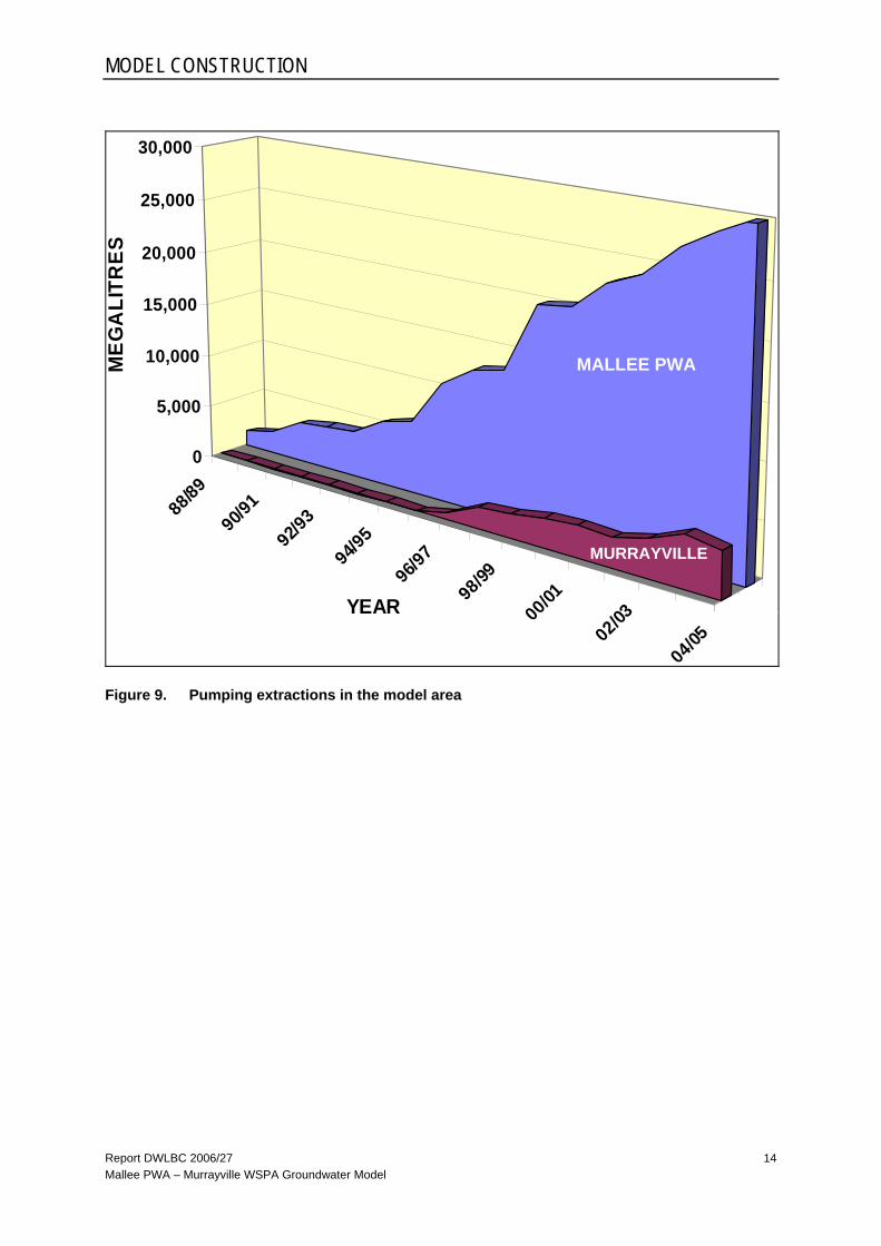
4.7 PUMPING DATA Irrigation wells in the study area were simulated using the MODFLOW WELL package. The design of the model grid ensures that each well is located at the centre of the cells. There was no pumping during the steady-state calibration. However during the transient calibration simulations, wells were ‘turned off’ in winter and ‘on’ in summer. Estimates of pumped volumes from all irrigation wells before 2002 were made using figures from irrigators (number of hours pumped x pumping rate). Since then, metered extractions have been available from virtually all irrigation bores in SA (Fig. 9). Metered volumes from the Murrayville WSPA were obtained from Mallee Wimmera Water. The location of the extraction points is shown in Figure 6.
MODEL CONSTRUCTION
Report DWLBC 2006/27 Mallee PWA – Murrayville WSPA Groundwater Model
14
88/89
90/9
1
92/9
3
94/9
5
96/9
7
98/99
00/01
02/03
04/05
S1S2
0
5,000
10,000
15,000
20,000
25,000
30,000
MEG
ALI
TRES
YEAR
Figure 9. Pumping extractions in the model area
MURRAYVILLE
MURRAYVILLE
MALLEE PWA
Report DWLBC 2006/27 Mallee PWA – Murrayville WSPA Groundwater Model
15
5. MODEL CALIBRATION
The groundwater flow models were calibrated by adjusting the value and distribution of the model input parameters so that the resulting model output matched the measured water levels and other hydrologic observations within an acceptable level of accuracy. Changes to the hydrogeologic parameter values were evaluated during the calibration processes to confirm that the changes implemented were within the acceptable range of variability of the parameters. After each change in model parameter value, model output was generated and compared with measured data to evaluate the effect of the selected parameter.
The model accuracy was calculated using the root mean square error (RMSE) comparison between water level measurements and simulated water levels. Model accuracy is increased as RMSE approaches zero. Average model error (AVER) was also used during model calibration processes to evaluate model bias, which occurs when the differences between simulated and observed water levels is predominantly positive or negative.
Trial-and-error method was used in the model calibrations. As the models were constructed, assumptions were necessary to reduce the model instability. The model was initially simplified but as the calibrations proceeded, complexity were systematically integrated into the model to improve the model output and to better represent the actual field conditions. The final steady-state model incorporates parameters that were modified during calibration of the transient model.
The models were considered calibrated when the following criteria were satisfied: • When incremental parameter changes in model input parameters did not result in a
smaller RMSE, and when AVER is close to zero.
• The RMSE is less than 0.5 m.
• The simulated groundwater potentiometric heads and lateral groundwater flow directions in the model compared favourably with those determined from water level measurements and published potentiometric surface maps of the Murray Group Limestone, Parilla Sands and Renmark Group aquifers.
• The simulated transient water levels fluctuations throughout the transient calibration period closely resembled measured water levels fluctuations resulting from the effects of variable (pumping) stresses through time.
5.1 STEADY-STATE MODEL CALIBRATION The steady-state model was calibrated by varying the following input model parameters (hydraulic conductivity and GHB conductance), within a specified range of reasonable values to obtain as close a match as possible between observed and simulated groundwater levels. Observed values included water levels measured for 1980 at 88 observation wells.
During the calibration process, improvements in the model output were evaluated by calculating the mean error (ME), the mean absolute error (MAE) and the root mean square error (RMSE) between the measured and simulated groundwater levels.

MODEL CALIBRATION
Report DWLBC 2006/27 Mallee PWA – Murrayville WSPA Groundwater Model
16
Table 3. Steady state calibration statistics
PS MGL RG
Points of comparison 13 69 8
Mean error (m) -0.05 0.01 0.03
Mean absolute error (m) 0.07 0.14 0.06
Root mean square error (m) 0.09 0.25 0.07
The mean error (ME) value for MGL of 0.01 indicated that water levels in MGL aquifer were overestimated to a very small degree. The scaled RMS error of 0.5% greatly exceeds the MDBC Modelling Guideline recommendations of 5%.
The differences between the observed and model-calculated heads are called the absolute residuals. Table 4 presents the residual statistics for the three aquifers. The mean difference between the observed and calculated heads in the MGL aquifer at the 71 observation wells (mean absolute residual) was 0.11 m. This value is less than 1 per cent of the simulated pre-development range in groundwater level elevation across the Mallee PWA (40 m). The absolute residual values indicate that the water levels in the MGL aquifer were not overestimated or underestimated to a large degree. However at some observation wells, differences of more than 0.3 m between observed and model-calculated heads occurred.
Table 4. Statistics of the absolute residuals
Parameter PS MGL RG
Number of observation wells 13 71 8
Minimum absolute residual value (m) 0.001 0.001 0.004
Maximum absolute residual value (m) 1.26 0.64 0.10
Range of absolute residuals (m) 1.26 0.63 0.09
Mean absolute residuals (m) 0.16 0.11 0.06
Median absolute residual value (m) 0.07 0.06 0.07
Standard error (m) 0.09 0.01 0.01
Average deviation (m) 0.18 0.09 0.03
Standard deviation (m) 0.34 0.11 0.04
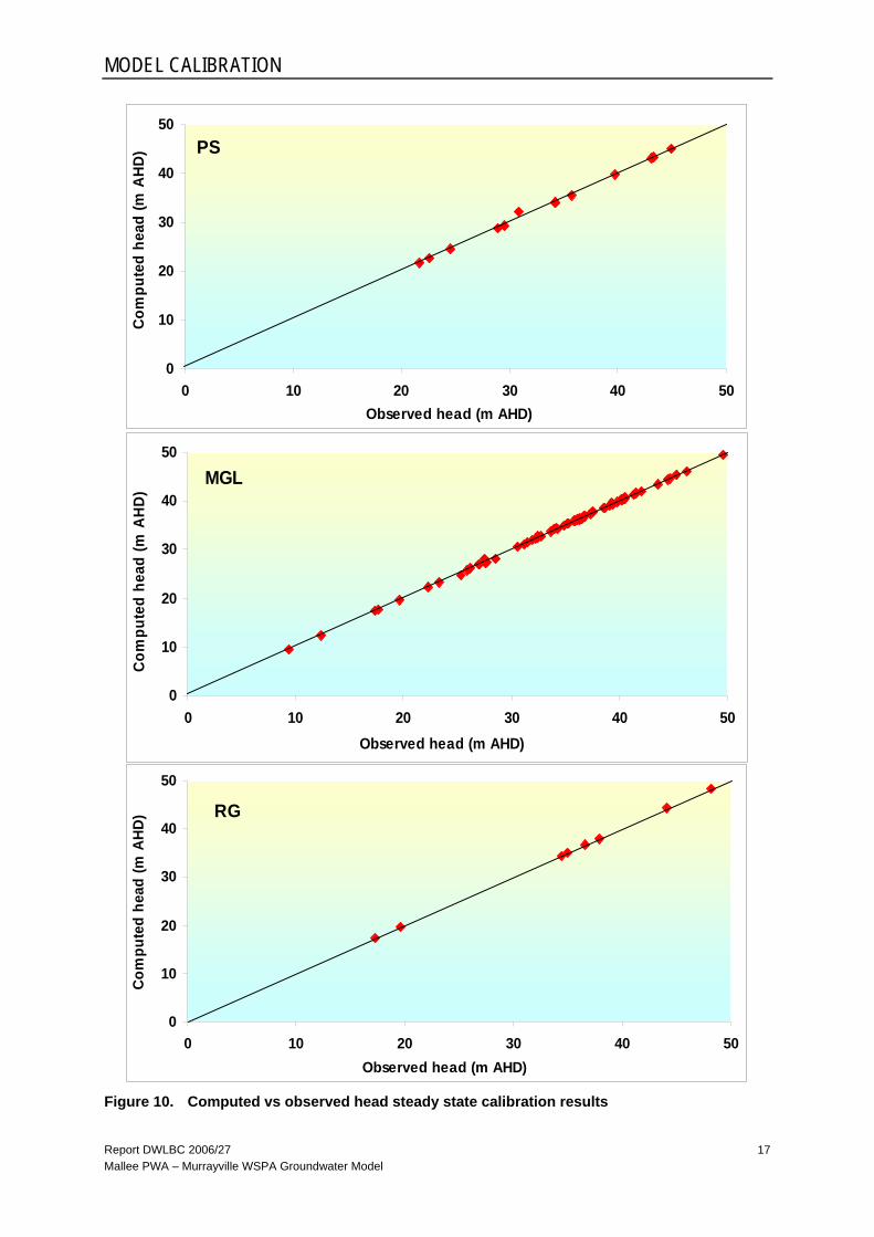
A graphical representation of the comparison between observed and calculated heads at observation wells in the three aquifers located throughout the model domain is presented in Figure 10. As can be seen, there is a very good match with all points lying close to the 1:1 line.
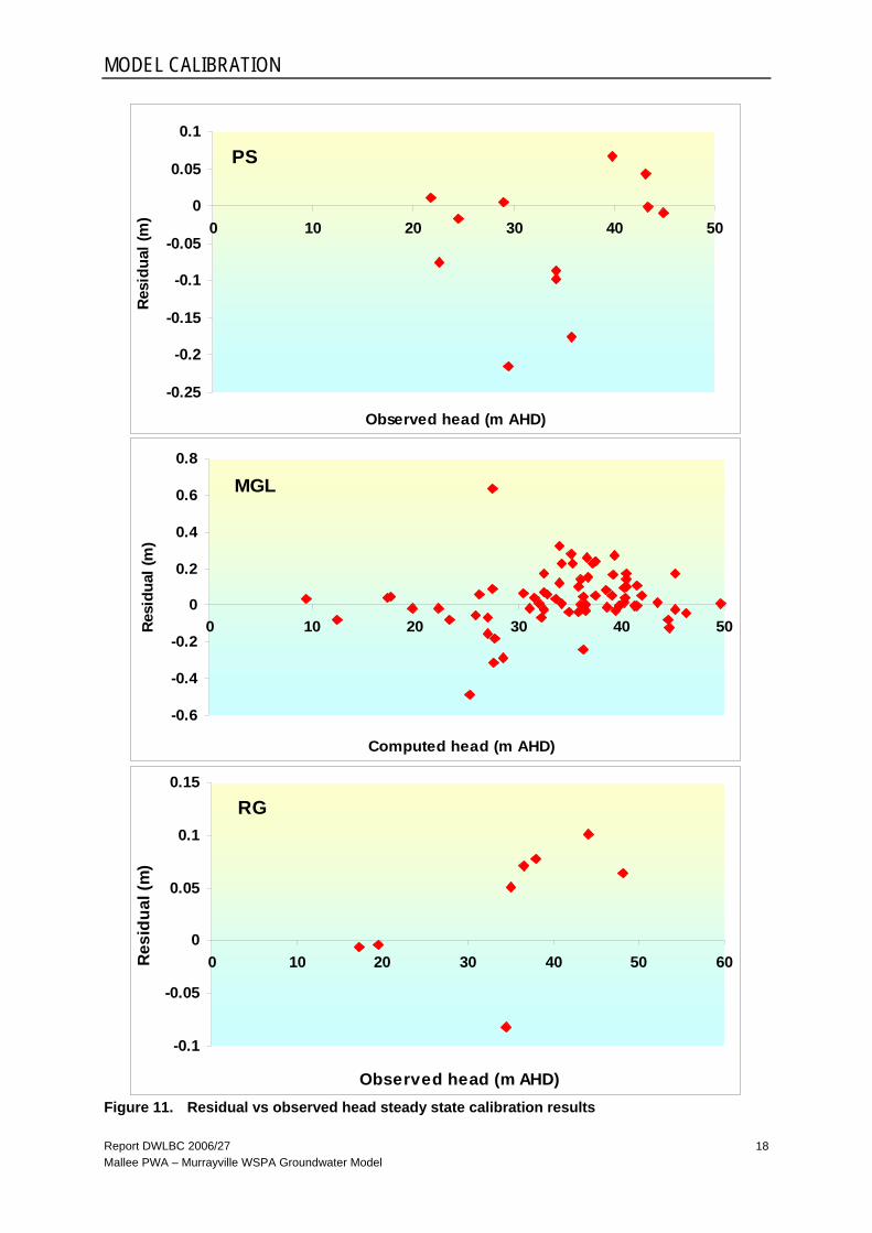
Figure 11 presents the residual (the difference between observed and calculated heads) plotted against the elevation of the water level at each observation well. Again, a very good calibration is indicated over most of the model domain.
MODEL CALIBRATION
Report DWLBC 2006/27 Mallee PWA – Murrayville WSPA Groundwater Model
17
PS
0
10
20
30
40
50
0 10 20 30 40 50Observed head (m AHD)
Com
pute
d he
ad (m
AH
D)
MGL
0
10
20
30
40
50
0 10 20 30 40 50Observed head (m AHD)
Com
pute
d he
ad (m
AH
D)
RG
0
10
20
30
40
50
0 10 20 30 40 50Observed head (m AHD)
Com
pute
d he
ad (m
AHD
)
Figure 10. Computed vs observed head steady state calibration results
MODEL CALIBRATION
Report DWLBC 2006/27 Mallee PWA – Murrayville WSPA Groundwater Model
18
PS
-0.25
-0.2
-0.15
-0.1
-0.05
0
0.05
0.1
0 10 20 30 40 50
Observed head (m AHD)
Res
idua
l (m
)
MGL
-0.6
-0.4
-0.2
0
0.2
0.4
0.6
0.8
0 10 20 30 40 50
Computed head (m AHD)
Resi
dual
(m)
RG
-0.1
-0.05
0
0.05
0.1
0.15
0 10 20 30 40 50 60
Observed head (m AHD)
Res
idua
l (m
)
Figure 11. Residual vs observed head steady state calibration results

MODEL CALIBRATION
Report DWLBC 2006/27 Mallee PWA – Murrayville WSPA Groundwater Model
19
Availability of piezometric data from the three aquifers allows comparison of vertical hydraulic gradients simulated in the steady state model. Tables 5 and 6 show the simulated difference in the head between the MGL and RG aquifers, and PS and MGL aquifers for selected sites where observation wells are completed in two aquifers. At some sites where pre-irrigation water levels were not available, values were obtained by extrapolating between pre-irrigation water level contours.
Table 5. Vertical hydraulic gradient between MGL and RG aquifers
Obs wells Aquifers Water Level (m AHD)
Observed (m)
Calculated (m) Direction
MND 10 MND 6
MGL RG
19.7 34.4
14.7 14.6 Upward
KNF 20 KNF 19
MGL RG
33.7 36.6
3.1 2.9 Upward
MMJ 1 MMJ 3
MGL RG
17.7 19.6
1.9 1.9 Upward
PNN 3 PNN 2
MGL RG
49.6 48.2
1.4 1.3 Downward
Table 6. Vertical hydraulic gradient between MGL and PS aquifers
Obs wells Aquifers Water Level (m AHD)
Observed (m)
Calculated (m) Direction
137201 137200
PS MGL
44.9 44.5
0.4 0.5 Downward
137199 137198
PS MGL
43.1 41.6
1.5 1.5 Downward
137197 82220
PS MGL
39.8 39.1
0.7 0.7 Downward
PEB 19 PEB 25
PS MGL
24.5 28.5
4.0 3.7 Upward
PEB 3 PEB 24
PS MGL
34.2 34.9
0.7 0.8 Upward
MCG 4 MCG 5
PS MGL
22.6 27.0
4.4 4.4 Upward
MCG 6 MCG 7
PS MGL
21.7 26.2
4.5 4.5 Upward
These tables show very good agreement between observed and calculated head differences, and gives confidence to the accuracy of leakage calculations between the aquifers.
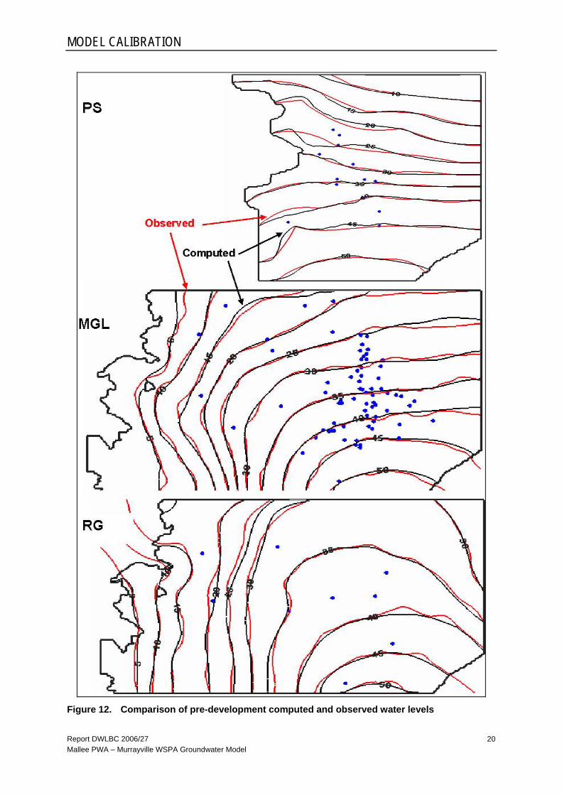
Comparisons of simulated and observed pre-development potentiometric surfaces in the MGL and RG aquifers are shown below in Figure 12, together with locations of observation wells used in the calibration process. In general, the simulated pre-development groundwater levels match the measured water levels quite well.
MODEL CALIBRATION
Report DWLBC 2006/27 Mallee PWA – Murrayville WSPA Groundwater Model
20
Figure 12. Comparison of pre-development computed and observed water levels
MODEL CALIBRATION
Report DWLBC 2006/27 Mallee PWA – Murrayville WSPA Groundwater Model
21
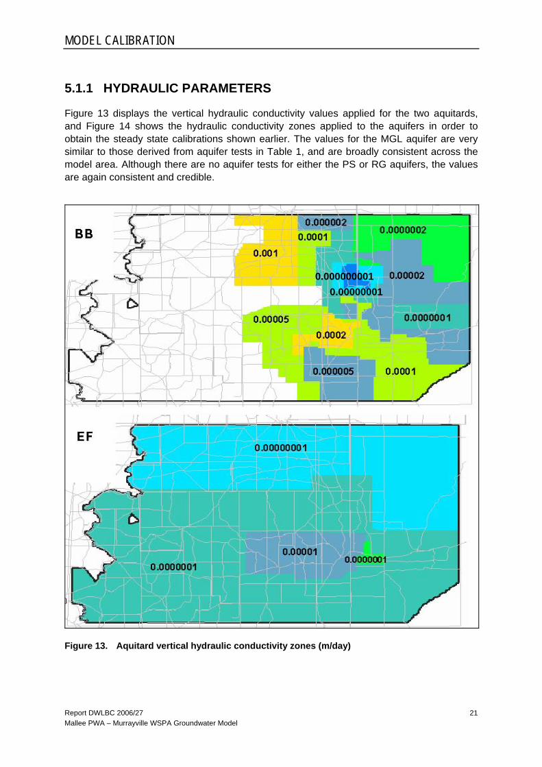
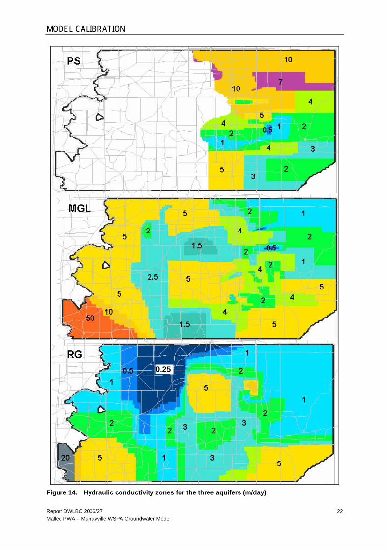
5.1.1 HYDRAULIC PARAMETERS
Figure 13 displays the vertical hydraulic conductivity values applied for the two aquitards, and Figure 14 shows the hydraulic conductivity zones applied to the aquifers in order to obtain the steady state calibrations shown earlier. The values for the MGL aquifer are very similar to those derived from aquifer tests in Table 1, and are broadly consistent across the model area. Although there are no aquifer tests for either the PS or RG aquifers, the values are again consistent and credible.
Figure 13. Aquitard vertical hydraulic conductivity zones (m/day)
0.00000001 0.000000001
MODEL CALIBRATION
Report DWLBC 2006/27 Mallee PWA – Murrayville WSPA Groundwater Model
22
Figure 14. Hydraulic conductivity zones for the three aquifers (m/day)
0.25

MODEL CALIBRATION
Report DWLBC 2006/27 Mallee PWA – Murrayville WSPA Groundwater Model
23
5.1.2 STEADY STATE SENSITIVITY ANALYSIS
A sensitivity analysis determines which parameters have the greatest effects on the results, by varying the model input parameters by several orders of magnitude while the remaining model parameters were held at the calibrated values.
The steady state model sensitivity was determined by varying the calibrated values of recharge and hydraulic conductivities (horizontal and vertical) of the aquifers and the confining beds, with results expressed in three statistical errors (expressed in metres) as show in Table 7.
Table 7. Sensitivity analyses of steady state input parameters
Multiples of HORIZONTAL HYDRAULIC CONDUCTIVITY Error
Aquifer 0.25 0.5 1.0 2.0 4.0
Mean error PS MGL RG
9.04 9.62 0.73
3.27 3.39 0.18
0.03 0.12 0.17
-1.65 -1.18 0.29
-2.5 -1.27 0.39
Absolute mean error
PS MGL RG
9.04 9.62 0.73
3.27 3.39 0.19
0.26 0.18 0.17
1.65 1.25 0.29
2.5 1.66 0.39
Root mean square error
PS MGL RG
9.21 10.16 1.03
3.32 3.62 0.24
0.29 0.21 0.22
1.71 1.44 0.36
2.62 1.99 0.49
The steady state model failed to converge when the calibrated horizontal hydraulic conductivity was multiplied by a factor of 0.1
Multiples of VERTICTAL HYDRAULIC CONDUCTIVITY Error
Aquifer 0.01 0.1 1.0 5.0 10.0
Mean error PS MGL RG
0.00 1.33 0.20
-0.39 0.92 0.20
0.03 0.12 0.17
0.02 -0.49 0.06
-0.04 -0.66 -0.04
Absolute mean error
PS MGL RG
1.65 1.33 0.20
0.90 0.92 0.20
0.26 0.18 0.17
0.48 0.50 0.09
0.57 0.68 0.12
Root mean square error
PS MGL RG
1.99 1.45 0.25
1.07 1.02 0.28
0.29 0.21 0.22
0.64 0.67 0.13
0.77 0.93 0.14
Multiples of RECHARGE Error
Aquifer 0.25 0.5 1.0 1.5 2.0
Mean error PS MGL RG
-3.10 -3.33 0.09
-2.05 -2.18 0.12
0.03 0.12 0.17
2.08 2.43 0.23
4.09 4.70 0.29
Absolute mean error
PS MGL RG
3.10 3.33 0.09
2.05 2.18 0.12
0.26 0.18 0.17
2.08 2.43 0.23
4.09 4.70 0.29
Root mean square error
PS MGL RG
3.18 3.42 0.14
2.12 2.24 0.17
0.29 0.21 0.22
2.12 2.49 0.29
4.16 4.81 0.36

MODEL CALIBRATION
Report DWLBC 2006/27 Mallee PWA – Murrayville WSPA Groundwater Model
24
The Root Mean Square Error (RMSE) was used to quantify the effect of a parameter change on the steady-state model results, and is plotted against the multiplication factor used to vary the parameter in Figure 15. These graphs show the simulated response of the MGL and RG aquifers to incremental changes in horizontal hydraulic conductivity, vertical hydraulic conductivity and recharge is shown (the PS aquifer response is virtually identical to that for the MGL).
When the input parameters are less than the calibrated values, horizontal hydraulic conductivity is very sensitive, followed by recharge and vertical hydraulic conductivity. When the input parameters are higher than the calibrated values, recharge is very sensitive, followed by horizontal hydraulic conductivity and vertical hydraulic conductivity. Of the three parameters tested, vertical hydraulic conductivity is the least sensitive.
0
2
4
6
8
10
12
0 1 2 3 4 5 6 7 8 9 10
Multiples of calibrated input values
Roo
t mea
n sq
uare
err
or (
m)
Multiples of hor hydr cond Multiples of vert hydr cond Multiples of recharge
0
0.2
0.4
0.6
0.8
1
1.2
0 1 2 3 4 5 6 7 8 9 10
Multiples of calibrated input values
Roo
t mea
n sq
uare
err
or (m
)
Figure 15. Sensitivity analyses for MGL and RG aquifers
MGL
RG

MODEL CALIBRATION
Report DWLBC 2006/27 Mallee PWA – Murrayville WSPA Groundwater Model
25
5.1.3 NON-UNIQUENESS
The only major difference with the previous Mallee model (Barnett and Yan, 2000) is the significant reapportioning of leakage into the MGL aquifer. Calibration was achieved with mostly downward leakage from the Bookpurnong Beds (BB) aquitard and comparatively little upward leakage from the RG aquifer - a reversal of the situation in the earlier model. This is the result of the low RG aquifer permeabilities encountered in the recently drilled RG observation well PEB 35, located in the area of intensive pumping on the border (Barnett, 2003). There is a possibility the low RG aquifer permeabilities encountered in PEB 35 are not representative, and additional stratigraphic information may result in a further reapportioning of leakage.
This problem of non-uniqueness commonly arises because many different possible sets of model inputs can produce nearly identical model outputs. In other words, multiple calibrations of the same system are possible using different combinations of boundary conditions and aquifer properties, because exact (“unique”) solutions cannot be computed when many variables are involved in the calibration approach. The MDBC Modelling Guidelines provides suggestions to reduce the non-uniqueness problem. • calibrating the model using hydraulic conductivity (and other) parameters that are
consistent with measured values
• calibrating to a range of hydrogeological conditions (eg. pumping) with the same parameter set.
Both these methods have been incorporated in this modelling exercise. In order to maintain credibility, the increased downward leakage condition has been used in all model scenarios because it is considered the worst case situation.
5.2 TRANSIENT MODEL CALIBRATION The transient model used the steady state results as the initial conditions, and carried out a simulation from the predevelopment situation in 1980, through to 2004. Each year was divided into two stress periods representing summer and winter seasons coinciding with the pumping and recovery periods. The winter stress period began in March/April and lasted for 155 days, with the summer stress period beginning in August/September and lasting 210 days. The exception was the 2002 drought year, when the winter period lasted only 100 days and summer 265 days, as a result of pumping starting earlier and lasting longer than normal. The summer and winter stress periods were divided into 7 and 5 time steps, respectively. It was assumed that there is no groundwater pumping during winter.
The transient model, which was calibrated to changes in water levels in response to recharge and pumping, was calibrated primarily by varying the storage properties within ranges of reasonable values to obtain a close match between simulated and measured water levels from 1983 to 2004. The recharge rates used in the transient model are the same as those used in the steady-state simulation.
Overall, the transient calibration results were considered to be very good. Figure 16 shows a typical comparison between the transient results and the observed hydrograph. More results from all three aquifers are shown in Appendix A. The model-calculated water level fluctuations generally correspond well with the observed seasonal high and low water levels.

MODEL CALIBRATION
Report DWLBC 2006/27 Mallee PWA – Murrayville WSPA Groundwater Model
26
PEB 24
10
15
20
25
30
35
1980 1985 1990 1995 2000 2005Date
Hea
d, m
AH
D
CalculatedObserved
Figure 16. Transient calibration result for MGL obs well PEB 24
To provide information on the performance of the model over time, RMS, MAE and ME, were calculated for the three aquifers (Fig. 17) over the whole calibration period. Statistics for the MGL aquifer, the only aquifer with pumping, are tabulated in Table 8.
Table 8. Transient calibration statistics for MGL aquifer (m)
Mean error Mean absolute error
Root mean square error
Minimum -3.63 1.25 1.97
Maximum 2.65 3.72 5.25
Mean 1.04 2.01 3.05
Median 1.73 1.78 2.74
Standard error 0.23 0.08 0.11
Average deviation 1.18 0.45 0.66
Standard deviation 1.65 0.57 0.81
Given the large drawdown induced by pumping (of the order of 10–15 m in some instances), the average of the mean absolute error is relatively small.
Another measure of average model error is the normalised RMS error (ratio between the RMS error and the total head loss). If the normalised RMS error value is small (less than 10% is usually the acceptable value), the model error is only a small part of the overall model response (Anderson and Woessner, 1992). The normalised RMS error ratio for 1980 to 2005 calibration for the MGL aquifer is about 7%, based on the total head loss across the modelled area of about 40 m and RMS error average of 3 m. The normalised RMS error ratio was determined to be small and therefore, judged to be acceptable.

MODEL CALIBRATION
Report DWLBC 2006/27 Mallee PWA – Murrayville WSPA Groundwater Model
27
-0.5
0
0.5
1
1980 1985 1990 1995 2000 2005Date
Erro
r (m
)mean error mean absolute error root mean square error
PLIOCENE SANDS
-4
-2
0
2
4
6
1980 1985 1990 1995 2000 2005Date
Erro
r (m
)
MURRAY GROUP LIMESTONE
-0.5
0
0.5
1
1980 1985 1990 1995 2000 2005Date
Erro
r (m
)
RENMARK GROUP
Figure 17. Transient calibration statistics over time
MODEL CALIBRATION
Report DWLBC 2006/27 Mallee PWA – Murrayville WSPA Groundwater Model
28
Even though these model errors are considered acceptable, they are mostly apparent errors caused by the fact that the closely matched modelled drawdowns and observed drawdowns (Fig. 16) occur at different times (the model assumes that extractions occur uniformly over the 210 day stress period commencing in August/September). Actual pumping often occurs only in the first or second half of this stress period in some areas.
5.2.1 HYDRAULIC PARAMETERS
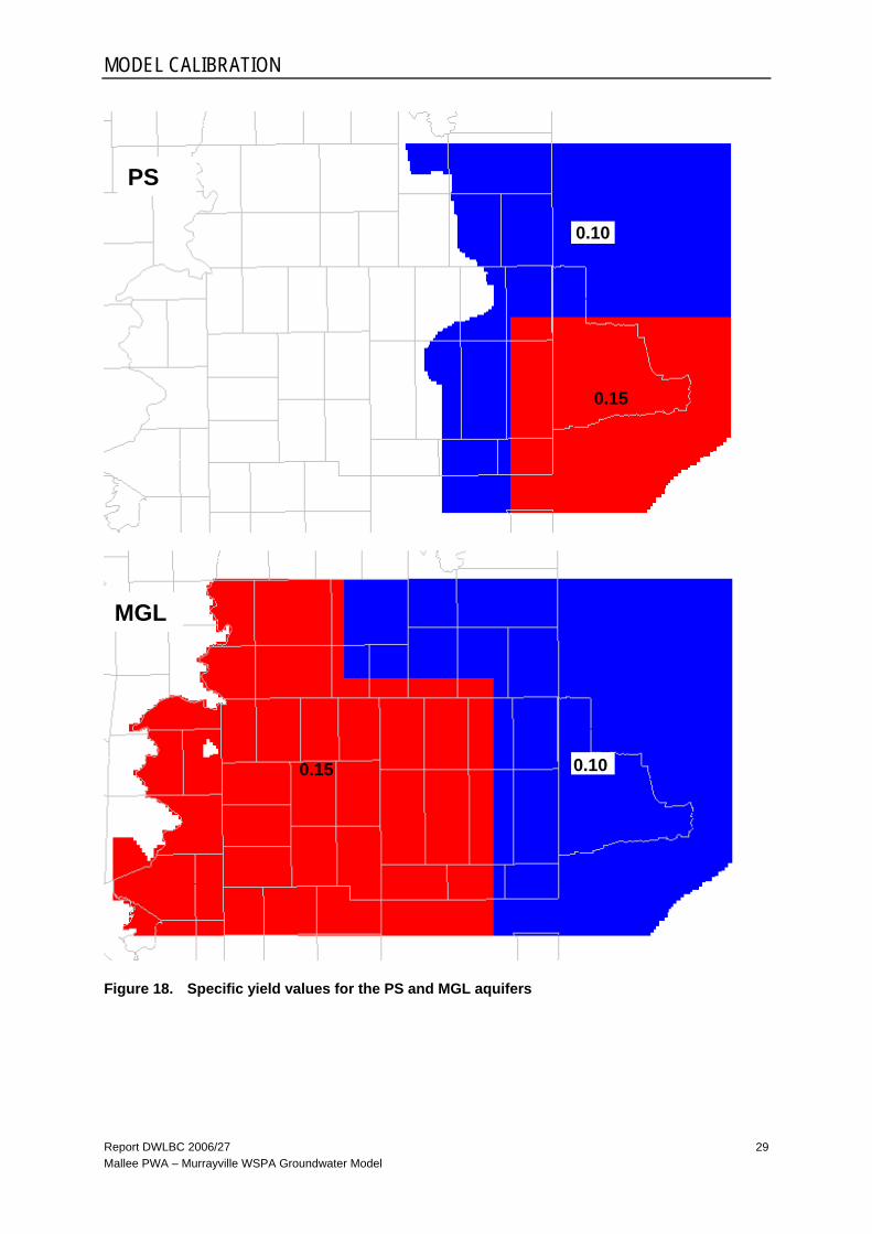
At the completion of the transient calibration, the following specific yield values were applied in the model (Fig. 18). Even though the MGL aquifer is confined over half the model area, a specific yield value is applied in case the aquifer becomes unconfined due drawdowns caused by pumping.
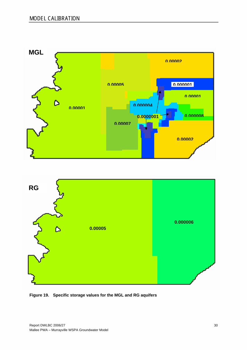
The specific storage values applied to confined portion of the MGL and RG aquifers are shown in Figure 19.
MODEL CALIBRATION
Report DWLBC 2006/27 Mallee PWA – Murrayville WSPA Groundwater Model
29
Figure 18. Specific yield values for the PS and MGL aquifers
0.15
PS
MGL
0.15 0.10
0.10
MODEL CALIBRATION
Report DWLBC 2006/27 Mallee PWA – Murrayville WSPA Groundwater Model
30
Figure 19. Specific storage values for the MGL and RG aquifers
0.00001
0.00002
0.00002
0.00005
0.00001
0.000008
0.000001
0.000004
0.000070.0000001
MGL
RG
0.00005 0.000006

MODEL CALIBRATION
Report DWLBC 2006/27 Mallee PWA – Murrayville WSPA Groundwater Model
31
5.2.2 TRANSIENT SENSITIVITY ANALYSIS
Analysis of the relative sensitivity of the transient model to various input hydraulic properties was carried out over the whole simulation period (from 1980 to 2005). The calibrated values of vertical (Kv) and horizontal (Kh) hydraulic conductivity values, and specific storage (Ss) were tested by multiplying and dividing them by 10. To test the sensitivity of specific yield (Sy), the calibrated values were multiplied by 0.1 and 2. The average root mean square errors in heads were plotted with change factor for specific yield, specific storage, vertical hydraulic conductivity and horizontal hydraulic of the MGL aquifer, and the vertical hydraulic conductivity of the Bookpurnong Formation and Ettrick Formation aquitards. Results are presented in Table 9.
Table 9. Average root mean square error for MGL aquifer (m)
Multiples of hydraulic properties Kh(MGL) Kv(MGL) Sy(MGL) Ss(MGL) Kv(BF) Kv(EF)
0.1 4.32 3.45 3.09 3.44 3.45 3.04
1 3.05 3.05 3.05 3.05 3.05 3.05
2
10 3.96 3.05 2.87 2.64 3.11
A change factor of 1, indicated by the vertical line in Figure 20 below, represents the value of the hydraulic property used in the calibrated model and corresponding average root mean square error. In comparison with other parameters tested, the transient model error is most sensitive to changes in horizontal hydraulic conductivity of the Murray Group Limestone (MGL) aquifer. However, the results show that overestimation or underestimation of any of the hydraulic parameters tested would not lead to any significant errors.
2.0
3.0
4.0
5.0
0.1 1 10Multiples of calibrated hydraulic parameters
Roo
t mea
n sq
uare
err
or (m
)
MGL(Kh) MGL(Ss) MGL(Kv) BF(Kv) MGL(Sy) EF(Kv)
Figure 20. Transient sensitivity analysis for the MGL aquifer
MODEL CALIBRATION
Report DWLBC 2006/27 Mallee PWA – Murrayville WSPA Groundwater Model
32
5.2.3 NON-UNIQUENESS
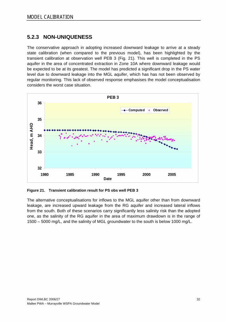
The conservative approach in adopting increased downward leakage to arrive at a steady state calibration (when compared to the previous model), has been highlighted by the transient calibration at observation well PEB 3 (Fig. 21). This well is completed in the PS aquifer in the area of concentrated extraction in Zone 10A where downward leakage would be expected to be at its greatest. The model has predicted a significant drop in the PS water level due to downward leakage into the MGL aquifer, which has has not been observed by regular monitoring. This lack of observed response emphasises the model conceptualisation considers the worst case situation.
PEB 3
32
33
34
35
36
1980 1985 1990 1995 2000 2005Date
Hea
d, m
AH
D
Computed Observed
Figure 21. Transient calibration result for PS obs well PEB 3
The alternative conceptualisations for inflows to the MGL aquifer other than from downward leakage, are increased upward leakage from the RG aquifer and increased lateral inflows from the south. Both of these scenarios carry significantly less salinity risk than the adopted one, as the salinity of the RG aquifer in the area of maximum drawdown is in the range of 1500 – 5000 mg/L, and the salinity of MGL groundwater to the south is below 1000 mg/L.
Report DWLBC 2006/27 Mallee PWA – Murrayville WSPA Groundwater Model
33
6. MODEL LIMITATIONS
It must be remembered that a groundwater model is a simplification of a complex natural system. As with all mathematical models of natural systems, the simplifications and assumptions incorporated into the models cause limitations in their appropriate uses and interpretations of simulation results. Some errors in the model results may occur where the simplifications do not adequately describe the complexity of the aquifer system.
Model input parameters (horizontal hydraulic conductivity, vertical hydraulic conductivity) specified for each active cell represent an average for the entire cell. The assumption of uniformity for entire cell introduces errors because of the heterogeneous nature and variability of the geologic materials.
The steady state model assumes that prior to 1980, inflows to the groundwater system were equal to outflows and that groundwater levels were stable. If this were not the case, the calibrated steady-state model would be incorrect, and water levels could have been rising or falling during the assumed steady-state conditions.
The boundary conditions used at the edges of the active model area were necessary to define how the modelled area interacts with the entire flow system. These boundaries are largely responsible for how flow occurs in the area and are a potential source of error in the modelling process.
Temporal and spatial scale also limits model use and accuracy. Hydrologic process and hydraulic stresses were represented in the transient model as seasonal averages, with simulation results presented as seasonal groundwater levels and flows. The model was not designed to simulate changes at shorter time scales (daily or monthly).
The spatial resolution of the simulation output was limited by the area of the grid cells. Water withdrawals and water level observations were averaged within grid cells and the exact locations of extraction wells were approximated to the centres of the cells. The head in each cell represents an average head for the aquifer in that cell, and is therefore a gross approximation of actual levels. In cells with high transmissivity values this is not a great problem, except if an observation well is located adjacent to a pumping well.
There is a lack of observed water level and aquifer test data around the southwest and northeast corners of the model area. Because the hydraulic parameters were not calibrated in these areas, the prediction results may be less accurate than the calibrated data rich areas.
Because the model structure employs horizontal layers, it is difficult to accurately represent steeply dipping strata, such as where the Bookpurnong Beds confining layer is draped over the Murrayville Monocline. Consequently, the model has predicted depressurisation in some areas where the pressure level is actually still well above the base of the confining layer. These erroneous results have been corrected where possible.
Probably the main limitation is the lack of accurate data on pumping volumes in SA before metering was introduced in 2002. These uncertainties may have led to a few calibration results not matching very well to observed water levels during this period.

MODEL LIMITATIONS
Report DWLBC 2006/27 Mallee PWA – Murrayville WSPA Groundwater Model
34
Despite these limitations, the model is very well calibrated and can be used with confidence to predict groundwater level and salinity trends, and to calculate flow budgets. However, it should not be expected to predict water level elevations at particular locations with an accuracy greater then 0.5 m.

Report DWLBC 2006/27 Mallee PWA – Murrayville WSPA Groundwater Model
35
7. WATER BALANCE
The results of the groundwater budget calculated for the Murray Group Limestone aquifer steady state condition are presented below in Table 10. In this table: • SA = Mallee PWA (including the expanded area to the west and Border Zones)
• Vic = Murrayville WSPA (including the Border Zones 10B and 11B
• SA BZ = Border Zones 10A and 11A within the Mallee PWA
• Vic BZ = Border Zones 10B and 11B within the Murrayville WSPA
Table 10. Groundwater budget for MGL aquifer (ML/year)
Flow component SA BZ Vic BZ SA Vic
INFLOW
Lateral inflow 975 700 1 880 1 565
Upward leakage from RG 310 40 500 45
Downward leakage from PS 845 325 3 500 510
Recharge 0 2 530 0
Inflow from Vic 380 380
Inlow from SA 20 20
TOTAL INFLOW 2 510 1 085 8 780 2 120
OUTFLOW
Lateral outflow 2 260 540 8100 1 560
Upward leakage into PS 180 160 600 175
Downward leakage into RG 50 5 60 5
Outflow to Vic 20 20
Outflow to SA 380 380
TOTAL OUTFLOW 2 510 1 085 8 780 2 120
Estimated aquifer storage (ML) 25 000 000 15 000 000 120 000 000 20 000 000
Table 10 shows the various flow components to be a very small proportion of the total volume of groundwater in storage in the modelled area, which has been calculated from the aquifer thickness and porosity. Because the steady state groundwater flow direction is in a northerly direction parallel to the border, the net cross border flow is only about 360 ML/yr from Victoria to SA.
The budget is also represented schematically in Figure 22 where net flows are presented. The figures in blue represent the numbers for the whole management areas, while the red figures represent the Border Zones only.

WATER BALANCE
Report DWLBC 2006/27 Mallee PWA – Murrayville WSPA Groundwater Model
36
Figure 22. Schematic steady state water balance for SA and Victoria (ML/yr)
7.1 DOWNWARD LEAKAGE Because of the perceived risk of salinity increases in the MGL aquifer due to downward leakage, the area where this leakage occurs and the predicted volumes will be presented in more detail. The determination of leakage (both upwards and downwards) in the pre-irrigation or steady state situation is difficult to determine accurately because of the lack of nested observation wells that were available at that time to provide actual head differences at the one location. Most of the observation wells in Victoria were established after irrigation commenced and hence cannot provide useful steady state data.
Figure 23 shows the estimated steady state leakage zones produced by the model, and the associated volumes in each State. As in Figure 22, the numbers in blue represent the numbers for the whole management areas, while the red numbers represent the Border Zones only. South of the black zero head difference contour, potential for downward leakage occurs from the PS to the MGL aquifer. In this area, the head difference is small, and the PS aquifer contains groundwater below 3000 mg/L. The risk from downward leakage in this area is negligible, because this steady state condition would have existed for hundreds or even thousands of years, but MGL salinities are still below 1000 mg/L. The Bookpurnong Beds confining layer must therefore act as an effective hydraulic barrier in this case.
540
700
35
360
775
260
2260
975 1560
180 335
2980
40
440 1880
8100
2530
1565
540 = Border zone only 1560 = Whole management area

WATER BALANCE
Report DWLBC 2006/27 Mallee PWA – Murrayville WSPA Groundwater Model
37
North of the black zero head difference contour, strong potential for upward leakage occurs from the MGL to the PS aquifer. In the area where irrigation extractions are occurring, low salinity groundwater below 1500 mg/L occurs. If upward or downward leakage is a significant process, this low salinity water would have potentially been leaking upwards for hundreds or even thousands of years, and therefore significant volumes could be stored in the overlying confining layer.
Figure 23. Extent of pre-irrigation leakage between the MGL and PS aquifers
500
165
0 0
+15
+10
+5
-1
-1
1.1.1.2 SA VI
Peebinga
Pinnaroo
160
770
3750 Murrayville
340 1110
335
+10 Contours of head difference (metres)

Report DWLBC 2006/27 Mallee PWA – Murrayville WSPA Groundwater Model
38
8. SCENARIO MODELLING
A number of modelling scenarios were proposed by the Border Agreement Review Committee. 1. Current extractions (2004–05) in both SA (30 660 ML/yr) and Victoria (4206 ML/yr).
2. Current PAV in SA (53 000 ML/yr) and current extractions in Victoria (4206 ML/yr).
3. Current allocations in SA (53 000 ML/yr) and full allocation in Victoria (9466 ML/yr).
4. Same extractions in SA and Vic Border Zones (at SA PAV rate of 16 000 ML/yr).
The starting point for these scenarios was the 2004–05 irrigation season. The extraction volumes in each scenario were applied in the following irrigation season and continued for 25 years until 2030. The results are presented (Figs 20–23) as seasonal drawdown (since 2005), water level elevation for the maximum drawdown during the pumping season, and water level elevation for the maximum recovery during the non-pumping season. These parameters are described below.
Typical hydrographs for the Border Zones are presented in Figures 24–26, with a more comprehensive presentation of hydrograph results in Appendix B.
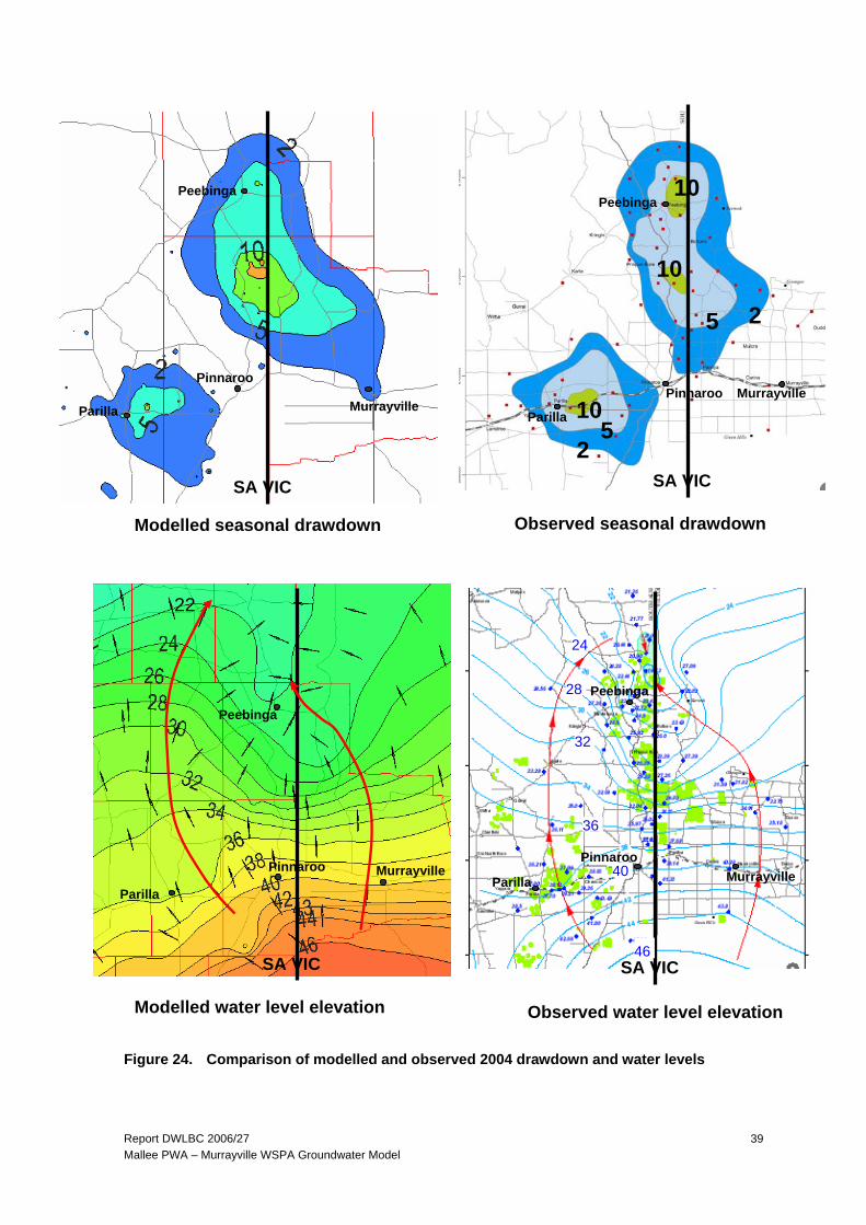
8.1 SCENARIO 1 This scenario models the current levels of extraction during the 2004–05 irrigation season. Figure 24 shows the comparison between the observed and modelled seasonal drawdown and water level elevation (maximum recovery) for 2004. There is generally good agreement, with discrepancies in the seasonal drawdown due to extrapolation between observation wells (red dots) in the observed contours, and the model assumption that all irrigation occurs continuously through the stress period.
These figures show the area of high seasonal drawdown straddles the border, with the maximum very close on the SA side. Groundwater flow is predominantly northwards through most of the Murrayville WSPA, until Zone 11B when it moves westward to SA.
It can be concluded that pumping in SA does not affect groundwater inflows into the Murrayville WSPA, and only groundwater that is not used in Victoria flows into SA. The cross-border flows during 2004–05 represent only 0.0001% of the volume of groundwater stored in the MGL aquifer in Zones 10B and 11B.
2005 2030
Water level
Seasonal drawdown Seasonal
drawdown
Max recovery elevation
Max drawdown elevation
Report DWLBC 2006/27 Mallee PWA – Murrayville WSPA Groundwater Model
39
Figure 24. Comparison of modelled and observed 2004 drawdown and water levels
Modelled seasonal drawdown Observed seasonal drawdown
Modelled water level elevation Observed water level elevation
Murrayville
Pinnaroo
Parilla
Peebinga
SA VIC
SA VIC
Murrayville Pinnaroo
Parilla
Peebinga
SA VIC
Pinnaroo Murrayville Parilla
Peebinga
46
40
36
32
28
24
22
Murrayville Pinnaroo
Parilla
Peebinga
SA VIC 2
25
5
10
10
10
SCENARIO MODELLING
Report DWLBC 2006/27 Mallee PWA – Murrayville WSPA Groundwater Model
40
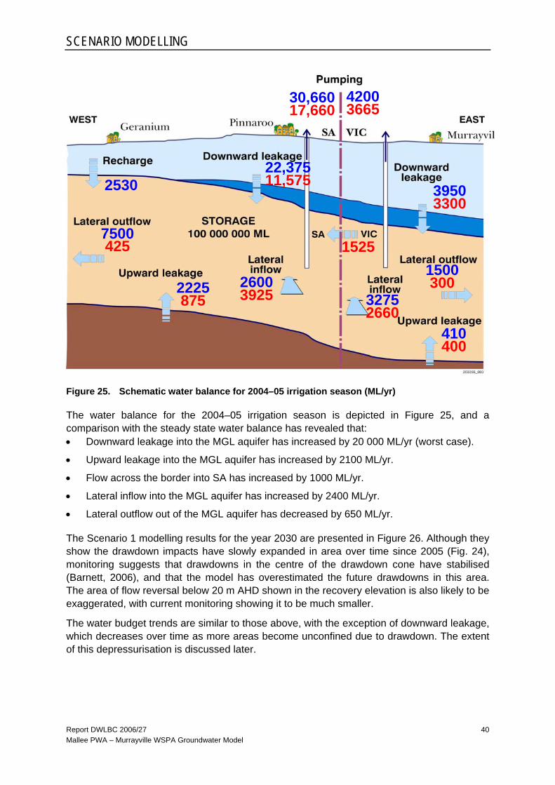
Figure 25. Schematic water balance for 2004–05 irrigation season (ML/yr)
The water balance for the 2004–05 irrigation season is depicted in Figure 25, and a comparison with the steady state water balance has revealed that: • Downward leakage into the MGL aquifer has increased by 20 000 ML/yr (worst case).
• Upward leakage into the MGL aquifer has increased by 2100 ML/yr.
• Flow across the border into SA has increased by 1000 ML/yr.
• Lateral inflow into the MGL aquifer has increased by 2400 ML/yr.
• Lateral outflow out of the MGL aquifer has decreased by 650 ML/yr.
The Scenario 1 modelling results for the year 2030 are presented in Figure 26. Although they show the drawdown impacts have slowly expanded in area over time since 2005 (Fig. 24), monitoring suggests that drawdowns in the centre of the drawdown cone have stabilised (Barnett, 2006), and that the model has overestimated the future drawdowns in this area. The area of flow reversal below 20 m AHD shown in the recovery elevation is also likely to be exaggerated, with current monitoring showing it to be much smaller.
The water budget trends are similar to those above, with the exception of downward leakage, which decreases over time as more areas become unconfined due to drawdown. The extent of this depressurisation is discussed later.
3300 3950
400 410
875 2225
11,575 22,375
2530
1525
17,660 30,660
3665 4200
300 1500
2660 3275 3925
2600
425 7500

SCENARIO MODELLING
Report DWLBC 2006/27 Mallee PWA – Murrayville WSPA Groundwater Model
41
8.2 SCENARIO 2 Scenario 2 requires full PAV extractions in SA, which requires a dramatic increase in pumping over most of Mallee PWA and Zone 11A, but a reduction in pumping in Zone 10A and Hd Parilla where licenced extractions are currently over the PAV. Figure 27 reflects these changes. The increase in pumping in the western part of the Mallee PWA has resulted in comparatively small increases in drawdown because the MGL aquifer is unconfined in this area. The drawdowns and groundwater flow directions in Victoria have changed little from Scenario 1.
The recovery elevation shows the area of flow reversal is greatly diminished, although the area of maximum pumping drawdown (and seasonal drawdown) has shifted north to Zone 11A in the vicinity of Peebinga.
8.3 SCENARIO 3 The extraction volumes in SA are the same as Scenario 2 and consequently, the seasonal drawdown and recovery elevations are very similar (Fig. 28). The increase in pumping in Victoria by 5300 ML/yr has moved the area of maximum drawdown further east to straddle the Border in Zones 11A and 11B, and also increased it by about 5 m. Most of the seasonal drawdown impact shifted over the Border into Victoria. The recovery elevation shows little change.
8.4 SCENARIO 4 This scenario involves a major increase in pumping in the Victorian Border Zones by a factor of 4–16 000 ML/yr in order to match the extractions in the SA Border Zones. It was assumed that the increased pumping would be distributed amongst the existing allocation holders.
Figure 29 shows a considerable increase in drawdown of about 5 m throughout the Victorian Border Zones, with a 2–3 m increase in the SA Border Zones. The maximum drawdown remains near Peebinga in Zone 11. The recovery elevation reveals a significant area of flow reversal in Zone 11.
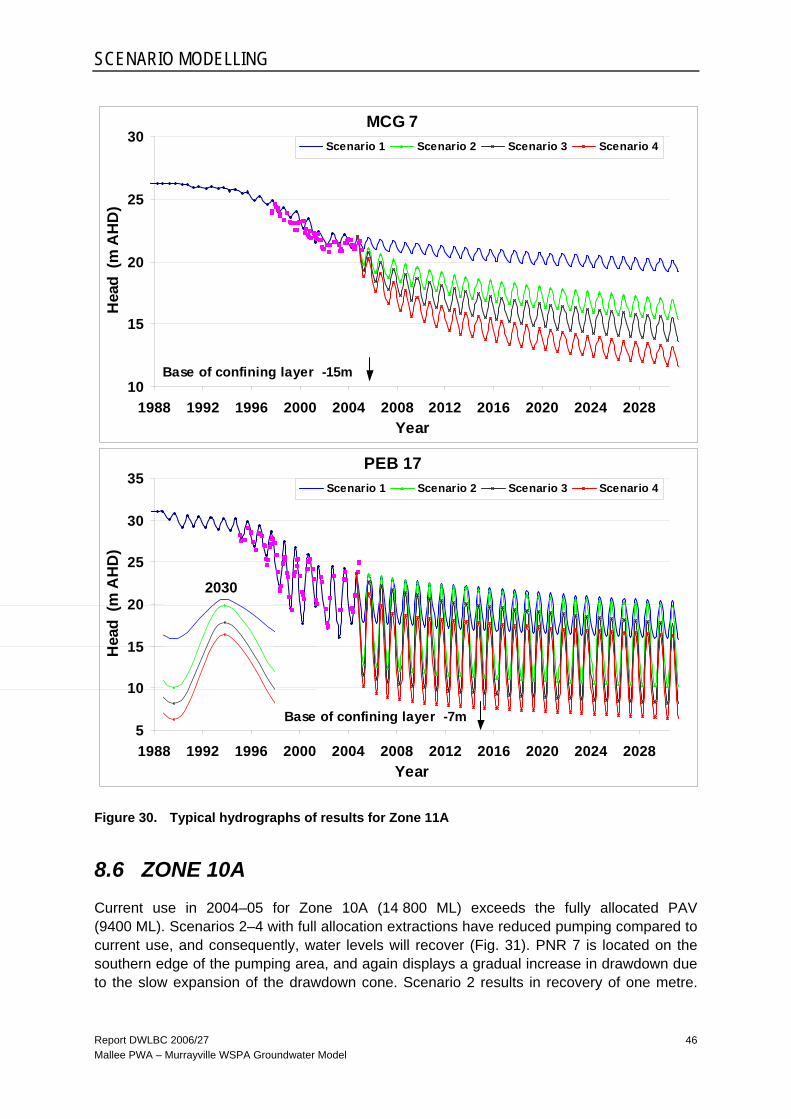
8.5 ZONE 11A Observation well MCG 7 is located on the northern edge of the pumping area. Scenario 1 (Fig. 30) shows a gradual increase in drawdown due to the slow expansion of the drawdown cone. Because of the higher salinities in Zone 11A, usage is well below the PAV although it is fully allocated. Consequently, Scenarios 2 and 3 (which assume full allocation pumping), show an increase in drawdown of 3 and 5 m respectively by 2030. As expected, the increase in pumping in Victoria in Scenario 4 produces a larger drawdown of 7 m at this site.
PEB 17 is located close to centre of pumping in Zone 11A. Drawdown has virtually reached an equilibrium. As for MCG 7, Scenarios 2 and 3 also have increased drawdown of 6 and 7 m respectively, as does increased pumping in Victoria (Scenario 4) with 10 m.
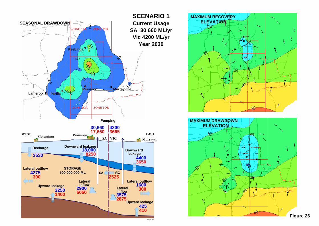
Figure 26. Scenario 1 results for 2030
SCENARIO 1 Current Usage
SA 30 660 ML/yr Vic 4200 ML/yr
Year 2030
MAXIMUM RECOVERY ELEVATION SEASONAL DRAWDOWN
ZONE 1OA ZONE 1OB
ZONE 11A ZONE 11B
Murrayville Pinnaroo Lameroo Parilla
Peebinga
MAXIMUM DRAWDOWN ELEVATION
3650 4400
300 1600
1400 3250 5050
2900
410 425
2875 3575
300 4275
8250 18,000
2530
17,660 30,660
3665 4200
Figure 26
2525
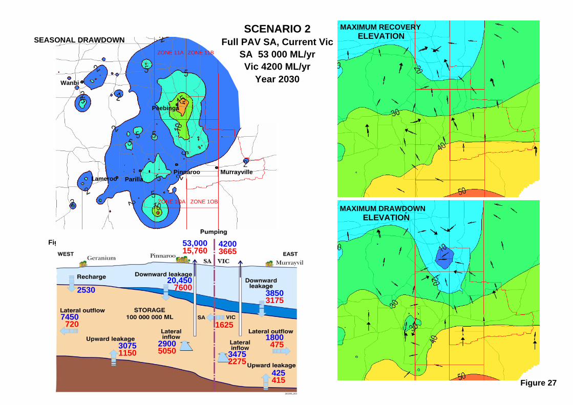
Figure 27. Scenario 2 results for 2030
ZONE 1OA ZONE 1OB
ZONE 11A ZONE 11B
Murrayville Pinnaroo Lameroo Parilla
Peebinga
SEASONAL DRAWDOWN SCENARIO 2
Full PAV SA, Current Vic SA 53 000 ML/yr Vic 4200 ML/yr
Year 2030 Wanbi
MAXIMUM RECOVERY ELEVATION
MAXIMUM DRAWDOWN ELEVATION
1150 3075
720 7450
415 425
2275 3475
3175 3850
475 1800
7600 20,450
5050 2900
2530
1625
15,760 53,000
3665 4200
Figure 27
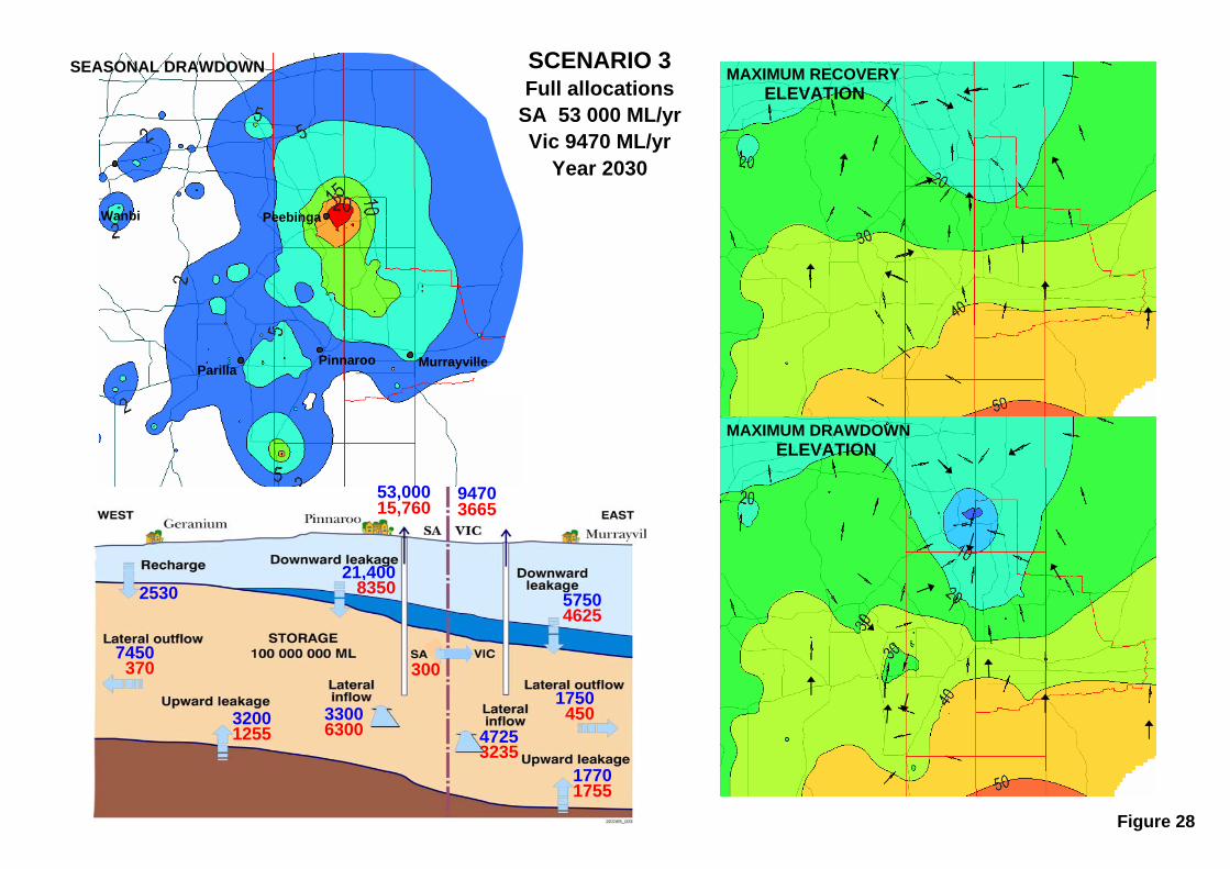
Figure 28. Scenario 3 results for 2030
Murrayville
SEASONAL DRAWDOWN
Pinnaroo Parilla
Peebinga
SCENARIO 3 Full allocations
SA 53 000 ML/yr Vic 9470 ML/yr
Year 2030
Wanbi
MAXIMUM DRAWDOWN ELEVATION
MAXIMUM RECOVERY ELEVATION
Figure 28
6300 3300
1755 1770
3235 4725
450 1750
370 7450
1255 3200
4625 5750
2530 8350 21,400
300
3665 9470
15,760 53,000

Figure 29. Scenario 4 results for 2030
SEASONAL DRAWDOWN
Wanbi
Murrayville Pinnaroo Parilla
Peebinga
MAXIMUM RECOVERY ELEVATION
MAXIMUM DRAWDOWN ELEVATION
SCENARIO 4 Same use in Border Zones
SA BZ 16 000 ML/yr Vic BZ 16 000 ML/yr
Year 2030
2530
2675
6975 3100 350
1825
6575 8200
325 7425
9100 22,400
15,760 53,000
16,300 17,620
Figure 29
1475 3450
5000 6175
2225 2250
SCENARIO MODELLING
Report DWLBC 2006/27 Mallee PWA – Murrayville WSPA Groundwater Model
46
Figure 30. Typical hydrographs of results for Zone 11A
8.6 ZONE 10A Current use in 2004–05 for Zone 10A (14 800 ML) exceeds the fully allocated PAV (9400 ML). Scenarios 2–4 with full allocation extractions have reduced pumping compared to current use, and consequently, water levels will recover (Fig. 31). PNR 7 is located on the southern edge of the pumping area, and again displays a gradual increase in drawdown due to the slow expansion of the drawdown cone. Scenario 2 results in recovery of one metre.
PEB 17
5
10
15
20
25
30
35
1988 1992 1996 2000 2004 2008 2012 2016 2020 2024 2028Year
Hea
d (m
AH
D)
Scenario 1 Scenario 2 Scenario 3 Scenario 4
Base of confining layer -7m
2030
MCG 7
10
15
20
25
30
1988 1992 1996 2000 2004 2008 2012 2016 2020 2024 2028Year
Hea
d (m
AH
D)
Scenario 1 Scenario 2 Scenario 3 Scenario 4
Base of confining layer -15m

SCENARIO MODELLING
Report DWLBC 2006/27 Mallee PWA – Murrayville WSPA Groundwater Model
47
Scenarios 3 and 4 involve increased pumping from Victoria close to this site, with increased drawdowns of up to 3 m.
PEB 24 is located in the centre of pumping, with Scenarios 2 and 3 resulting in a recovery of up to 5 m from current levels.
Figure 31. Typical hydrographs of results for Zone 10A
PEB 24
0
10
20
30
40
1988 1992 1996 2000 2004 2008 2012 2016 2020 2024 2028Year
Hea
d (m
AH
D)
Scenario 1 Scenario 2 Scenario 3 Scenario 4
Base of confining layer 6m
2030
PNR 7
22
27
32
37
42
1988 1992 1996 2000 2004 2008 2012 2016 2020 2024 2028Year
Hea
d (m
AH
D)
Scenario 1 Scenario 2 Scenario 3 Scenario 4
Base of confining layer 25m
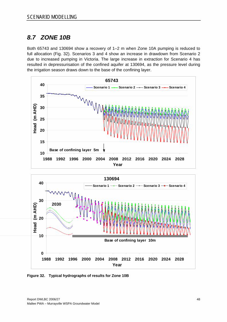
SCENARIO MODELLING
Report DWLBC 2006/27 Mallee PWA – Murrayville WSPA Groundwater Model
48
8.7 ZONE 10B Both 65743 and 130694 show a recovery of 1–2 m when Zone 10A pumping is reduced to full allocation (Fig. 32). Scenarios 3 and 4 show an increase in drawdown from Scenario 2 due to increased pumping in Victoria. The large increase in extraction for Scenario 4 has resulted in depressurisation of the confined aquifer at 130694, as the pressure level during the irrigation season draws down to the base of the confining layer.
65743
10
15
20
25
30
35
40
1988 1992 1996 2000 2004 2008 2012 2016 2020 2024 2028Year
Hea
d (m
AH
D)
Scenario 1 Scenario 2 Scenario 3 Scenario 4
Base of confining layer 5m
Figure 32. Typical hydrographs of results for Zone 10B
130694
0
10
20
30
40
1988 1992 1996 2000 2004 2008 2012 2016 2020 2024 2028Year
Hea
d (m
AH
D)
Scenario 1 Scenario 2 Scenario 3 Scenario 4
Base of confining layer 10m
2030
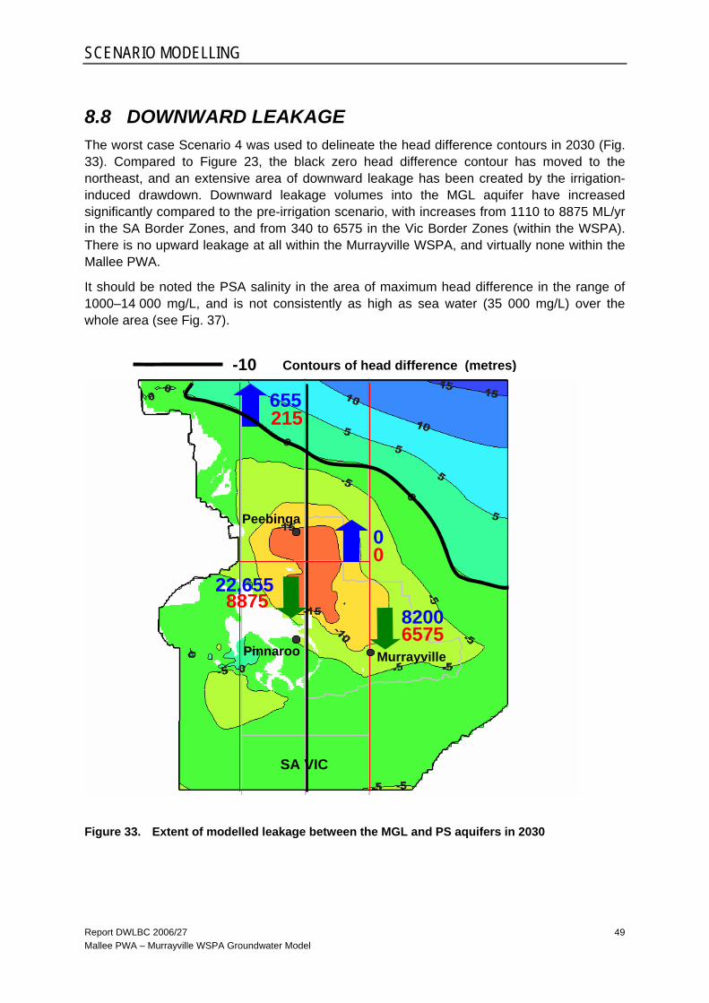
SCENARIO MODELLING
Report DWLBC 2006/27 Mallee PWA – Murrayville WSPA Groundwater Model
49
8.8 DOWNWARD LEAKAGE The worst case Scenario 4 was used to delineate the head difference contours in 2030 (Fig. 33). Compared to Figure 23, the black zero head difference contour has moved to the northeast, and an extensive area of downward leakage has been created by the irrigation-induced drawdown. Downward leakage volumes into the MGL aquifer have increased significantly compared to the pre-irrigation scenario, with increases from 1110 to 8875 ML/yr in the SA Border Zones, and from 340 to 6575 in the Vic Border Zones (within the WSPA). There is no upward leakage at all within the Murrayville WSPA, and virtually none within the Mallee PWA.
It should be noted the PSA salinity in the area of maximum head difference in the range of 1000–14 000 mg/L, and is not consistently as high as sea water (35 000 mg/L) over the whole area (see Fig. 37).
Figure 33. Extent of modelled leakage between the MGL and PS aquifers in 2030
SA VIC
Peebinga
Pinnaroo
0
655
22,655
Murrayville 6575
8875
215
8200
0
-10 Contours of head difference (metres)

SCENARIO MODELLING
Report DWLBC 2006/27 Mallee PWA – Murrayville WSPA Groundwater Model
50
8.9 DEPRESSURISATION Depressurisation of a confined aquifer occurs when its pressure level falls below the base of the confining layer (ie the top of the aquifer). This process has been modelled in Figure 32. The large seasonal drawdown fluctuations gradually reduce until the water level stays permanently below the top of the MGL aquifer, which then becomes unconfined.
As a result of depressurisation, seasonal drawdowns will be much smaller because they will be caused by the slow groundwater flow through the aquifer material, rather than an instantaneous pressure response. Downward leakage fluxes will also be reduced by the creation of an unsaturated zone below the confining layer. An example of this drawdown response is shown in Figure 34, which displays water levels from MPA 109 located in the Northern Adelaide Plains.
Figure 35 shows the estimated extent of the unconfined portion of the MGL aquifer for each of the modelling scenarios. Not surprisingly, they occur mostly in the centres of concentrated pumping. Depressurisation also occurs where the confining layer is very thin (1–2 m) to the south of Pinnaroo. There are no adverse consequences here because the overlying Pliocene Sands unit is dry.
20
30
40
50
60
701987 1990 1992 1995 1998 2001 2003 2006
Year
Dep
th to
wat
er (m
)
Figure 34. Example of depressurisation in the Northern Adelaide Plains
Base of confining layer
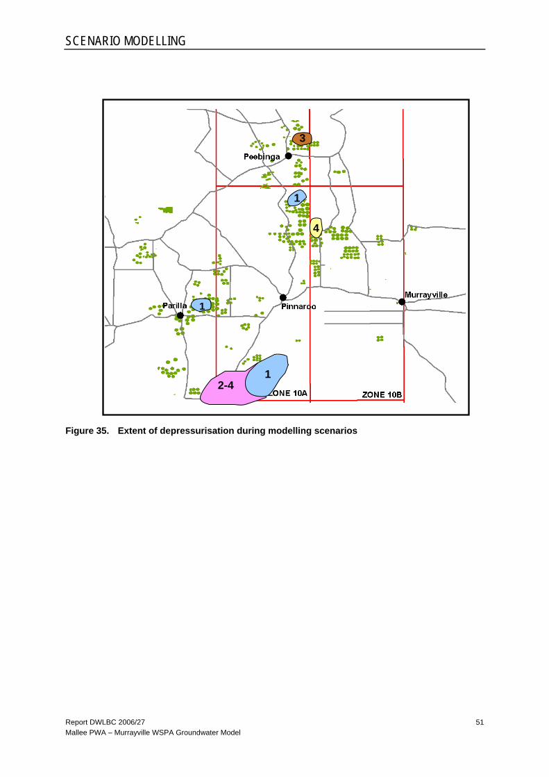
SCENARIO MODELLING
Report DWLBC 2006/27 Mallee PWA – Murrayville WSPA Groundwater Model
51
Figure 35. Extent of depressurisation during modelling scenarios
1
1
1 2-4
3
4

Report DWLBC 2006/27 Mallee PWA – Murrayville WSPA Groundwater Model
52
9. SALINITY MODELLING
MT3D-MS was used to simulate changes in groundwater salinity in the MGL aquifer as a result of inter-aquifer leakage induced by groundwater extractions. MT3D-MS is a modular three-dimensional multi-species computer program designed to model contaminant transport based on a pre-solved groundwater flow model (MODFLOW was used to solve the groundwater flow equations).
MT3D-MS can be used to simulate changes in concentrations of soluble components in groundwater taking into account advection, dispersion, diffusion and simple chemical reactions, with various types of boundary conditions and external sources or sinks. The model can accommodate very general spatial discretization schemes and transport boundary conditions, including: • Confined, unconfined or variably confined/unconfined aquifer layers.
• Specified concentration or mass flux boundaries.
• Transport effects of external hydraulic sources and sinks such as wells, drains, rivers, areal recharge and evapotranspiration.
The following data were used in the model: • Observed salinity hydrographs from observation wells in the modelled area.
• Salinity contour maps representing the steady state salinity condition.
• Groundwater extraction data.
The following assumptions were made for the model construction: • The solute modelled was assumed to be conservative.
• The transport of the conservative solute is affected only by advection and dispersion.
• Groundwater flow is the only force that determines the transport of the solute.
• There are no adsorption or reactions affecting the solute.
The salinity model was developed in three stages: 1. Pre 1980 steady state model to establish initial conditions for the transient model.
2. Calibrated transient model for the period from 1980 to 2005.
3. Predictive models examining the impact of various pumping scenarios on groundwater salniity in the MGL aquifer.
9.1 BOUNDARY CONDITIONS The boundary conditions used in the transport modelling included constant concentration, general head concentration and no-transport boundaries. These boundaries coincided with the boundaries used in the flow model, and are shown in Figure 36.
The spatial and temporal divisions of the solute transport simulation followed those of the flow model. The grid used to solve the transport equations was also the same as that of the flow model.
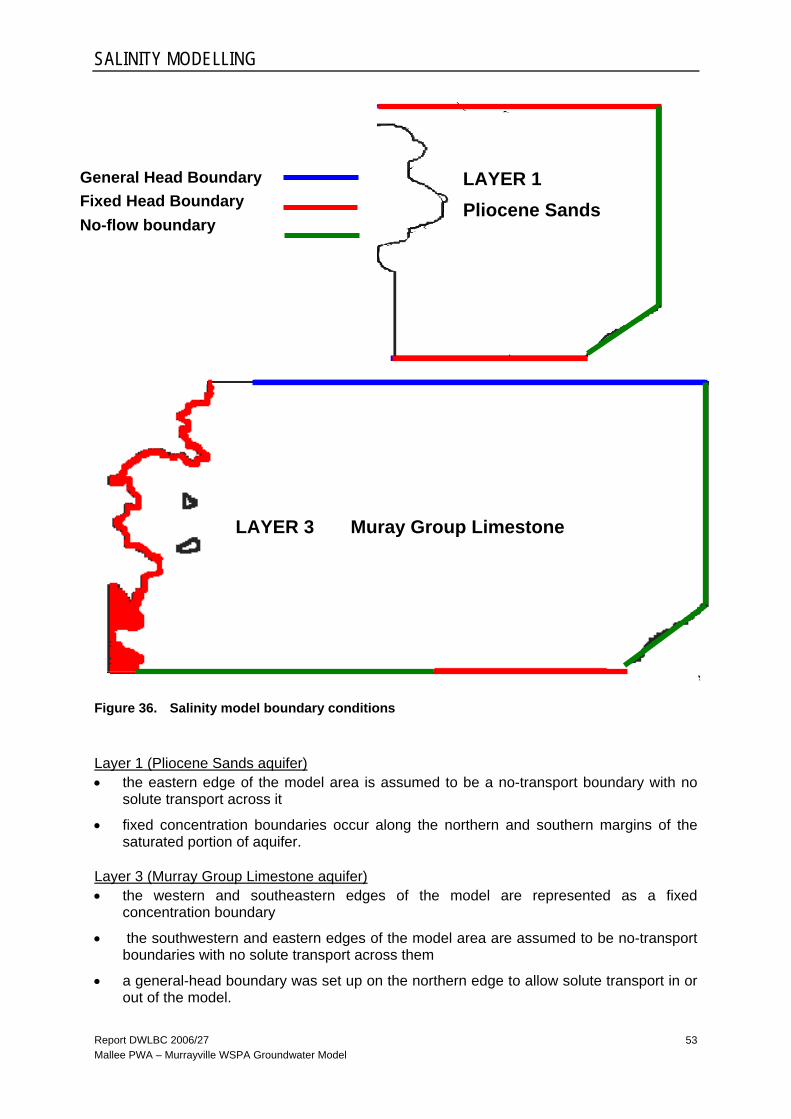
SALINITY MODELLING
Report DWLBC 2006/27 Mallee PWA – Murrayville WSPA Groundwater Model
53
Figure 36. Salinity model boundary conditions
Layer 1 (Pliocene Sands aquifer) • the eastern edge of the model area is assumed to be a no-transport boundary with no
solute transport across it
• fixed concentration boundaries occur along the northern and southern margins of the saturated portion of aquifer.
Layer 3 (Murray Group Limestone aquifer) • the western and southeastern edges of the model are represented as a fixed
concentration boundary
• the southwestern and eastern edges of the model area are assumed to be no-transport boundaries with no solute transport across them
• a general-head boundary was set up on the northern edge to allow solute transport in or out of the model.
LAYER 3 Muray Group Limestone
LAYER 1 Pliocene Sands
General Head Boundary Fixed Head Boundary No-flow boundary

SALINITY MODELLING
Report DWLBC 2006/27 Mallee PWA – Murrayville WSPA Groundwater Model
54
9.2 INITIAL SALINITY AND INPUT PARAMETERS Downward leakage into the MGL aquifer could occur directly from the Bookpurnong Beds confining layer and ultimately, from the overlying Pliocene Sands aquifer after a very long period of time. Because the salinity distribution in the confining layer is not known, it was assumed to be the same as the overlying Pliocene Sands aquifer. This approach is conservative because significant upward leakage of low salinity water from the MGL could have occurred for many years before irrigation commenced.
Figure 37. Initial model salinity concentrations
MGL
PS
S ALINITY50 0 - 1 0 00 m g /L
10 0 0 - 1 50 0
15 0 0 - 3 00 0
30 0 0 - 7 00 0
70 0 0 - 1 40 0 0
14 0 0 0 - 35 0 00
> 3 50 0 0

SALINITY MODELLING
Report DWLBC 2006/27 Mallee PWA – Murrayville WSPA Groundwater Model
55
The salinity concentrations of the PS and MGL aquifers in the study area were used as a baseline for the groundwater salinity simulation. These initial salinity concentrations were based on the Murray Basin Hydrogeological Mapping salinity contours, which were updated by more recent sampling (eg SKM, 2004), and observed salinity values at observation wells as shown in Figure 37. The model has linearly interpolated salinity values in the aquifer between the contours by using the Kriging method.
Transport parameters used in the model are listed in Table 11. Since no transport parameters have been determined for the aquifer systems in the study area, these parameters included were based on a compilation of values from a range of field and laboratory studies in Waterloo Hydrogeologic, Inc, EnviroBrowser Lite Version 3.1 (August 2002). A series of simulations were run and outputs analysed to help determine what dispersivity values from the published literature were representative. Longitudinal dispersivity is typically greater than transverse and vertical dispersivity. In this modelling exercise, it was assumed that tranverse dispersivity is one-hundredth the longitudinal dispersivity and vertical dispersivity is one-thousandth the longitudinal dispersivity.
Table 11. Solute transport parameters
Layer Transport parameter
1 2 3 4 5 Effective porosity 0.1–0.5 0.4 0.25 0.3 0.3
Longitudinal dispersivity (m) 1 3 11.6 3 1
Transverse dispersivity (m) 0.01 0.03 0.116 0.03 0.01
Vertical dispersivity (m) 0.001 0.003 0.0116 0.003 0.001
Diffusion coefficient (m2/d) 0.00001 0.00001 0.00001 0.00001 0.00001
9.3 SALINITY MODEL CALIBRATION Both steady and transient salinity models were run under advective transport with dispersion and diffusion. Calibrations were achieved by adjustment of transport parameters to produce: • Simulated salinity concentration with salinity distributions similar to the observed.
• Calibration comparable with salinity concentrations at observation wells.
The solution behaviour of the transport models was checked for convergence of flow and salinity solution, stability and mass balance. The steady state salinity model converged to 1.75% mass discrepancy when the upstream weighing Standard Finite Method solver was used. The MDBC Modelling Guidelines do not have specific solute transport standards.
To produce a reasonable concentration distribution as initial conditions for the transient state transport simulations, a steady state MT3D-MS simulation was run. During the steady state calibration run, the initial transport parameters obtained from the literature were adjusted until an acceptable match with the observed salinity concentrations at monitoring sites was achieved. The result of the steady state run showing a steady-state concentration distribution is shown in Figure 38.
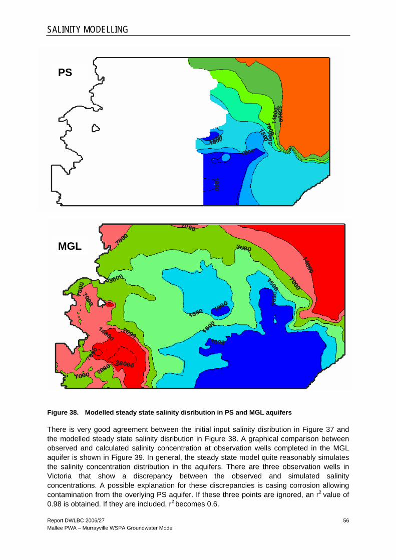
SALINITY MODELLING
Report DWLBC 2006/27 Mallee PWA – Murrayville WSPA Groundwater Model
56
Figure 38. Modelled steady state salinity disribution in PS and MGL aquifers
There is very good agreement between the initial input salinity disribution in Figure 37 and the modelled steady state salinity disribution in Figure 38. A graphical comparison between observed and calculated salinity concentration at observation wells completed in the MGL aquifer is shown in Figure 39. In general, the steady state model quite reasonably simulates the salinity concentration distribution in the aquifers. There are three observation wells in Victoria that show a discrepancy between the observed and simulated salinity concentrations. A possible explanation for these discrepancies is casing corrosion allowing contamination from the overlying PS aquifer. If these three points are ignored, an r2 value of 0.98 is obtained. If they are included, r2 becomes 0.6.
MGL
PS
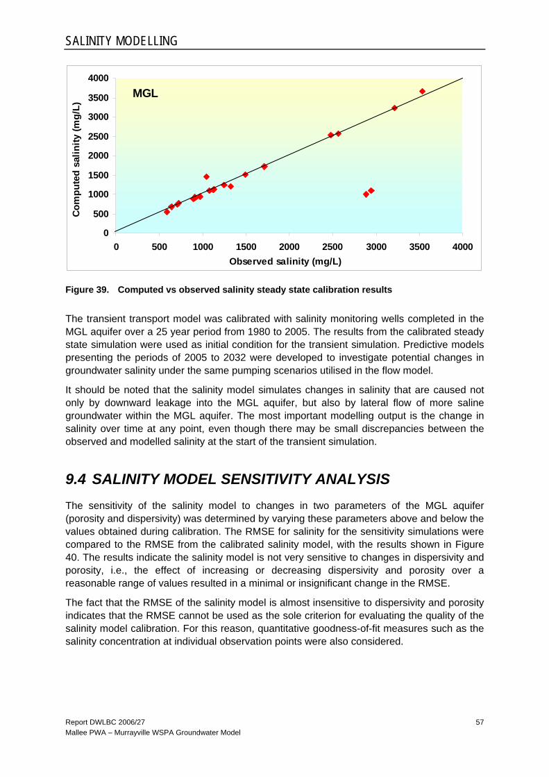
SALINITY MODELLING
Report DWLBC 2006/27 Mallee PWA – Murrayville WSPA Groundwater Model
57
MGL
0
500
1000
1500
2000
2500
3000
3500
4000
0 500 1000 1500 2000 2500 3000 3500 4000Observed salinity (mg/L)
Com
pute
d sa
linity
(mg/
L)
Figure 39. Computed vs observed salinity steady state calibration results
The transient transport model was calibrated with salinity monitoring wells completed in the MGL aquifer over a 25 year period from 1980 to 2005. The results from the calibrated steady state simulation were used as initial condition for the transient simulation. Predictive models presenting the periods of 2005 to 2032 were developed to investigate potential changes in groundwater salinity under the same pumping scenarios utilised in the flow model.
It should be noted that the salinity model simulates changes in salinity that are caused not only by downward leakage into the MGL aquifer, but also by lateral flow of more saline groundwater within the MGL aquifer. The most important modelling output is the change in salinity over time at any point, even though there may be small discrepancies between the observed and modelled salinity at the start of the transient simulation.
9.4 SALINITY MODEL SENSITIVITY ANALYSIS The sensitivity of the salinity model to changes in two parameters of the MGL aquifer (porosity and dispersivity) was determined by varying these parameters above and below the values obtained during calibration. The RMSE for salinity for the sensitivity simulations were compared to the RMSE from the calibrated salinity model, with the results shown in Figure 40. The results indicate the salinity model is not very sensitive to changes in dispersivity and porosity, i.e., the effect of increasing or decreasing dispersivity and porosity over a reasonable range of values resulted in a minimal or insignificant change in the RMSE.
The fact that the RMSE of the salinity model is almost insensitive to dispersivity and porosity indicates that the RMSE cannot be used as the sole criterion for evaluating the quality of the salinity model calibration. For this reason, quantitative goodness-of-fit measures such as the salinity concentration at individual observation points were also considered.

SALINITY MODELLING
Report DWLBC 2006/27 Mallee PWA – Murrayville WSPA Groundwater Model
58
-1
-0.5
0
0.5
1
0 5 10 15 20
Multiples of calibrated longitudinal dispersivity values
Dev
iatio
n fr
om c
alib
rate
d R
MSE
(mg/
L)
-0.001
0
0.001
0.002
0.003
0 0.5 1 1.5 2
Multiples of calibrated porosity values
Dev
iatio
n fr
om c
alib
rate
d R
MSE
(mg/
L)
Figure 40. Salinity model sensitivity analysis for the MGL aquifer
9.5 SALINITY MODEL LIMITATIONS There is no available information on any of the key parameters of dispersivity and diffusion for the MGL aquifer to assist with the calibration, and no data on the salinity distribution in the Bookpurnong Beds confining layer, or the upper MGL aquifer.
The model was not designed specifically for solute transport simulations, and consequently the coarse grid and large MGL aquifer thickness (~100 m) would probably allow too much dilution for reliable predictions of the impacts of any downward leakage. In the areas of concentrated pumping, the numerous fully penetrating irrigation bores may induce significant mixing of aquifer water. Because of these shortcomings, the salinity model should not be the prime tool for assessing salinity risk due to downward leakage.
However, the impacts of lateral flow of more saline groundwater within the MGL aquifer can be modelled with some confidence.
SALINITY MODELLING
Report DWLBC 2006/27 Mallee PWA – Murrayville WSPA Groundwater Model
59
9.6 RESULTS Figure 41 shows some results from SA. Bore PEB 24 is located in Zone 10A very close to the area of maximum seasonal drawdown where downward leakage is greatest. It shows a maximum increase of 40 mg/L over 25 years at current pumping rates (Scenario 1). This represents an increase of only 4%, and is within the range of current monitoring variations. Bore MCG 7 is located in Zone 11A and is within the area of flow reversal identified in Barnett (2006), where the risk of salinity increase is greatest due to lateral flow of more saline groundwater from the north. Here, a maximum increase of only 15 mg/L (0.08%) over 25 years is observed. More results are shown in Appendix C.
Similarly, Figure 42 shows representative results from Victoria. Bore 77199 is close to the area of maximum downward leakage, yet shows no increase in salinity over 25 years. Bore 49679 is situated where groundwater flow is turning northwest and where the risk of salinity rise due to lateral flow of more saline groundwater from the east, is increasing. Although other bores show a better calibration than Bore 49679, the modelled salinity response at its location is the important factor. The results again show no increase in salinity. Other salinity prediction results are presented in Appendix C.

Figure 41. Salinity predictions in SA
PEB 24
700
800
900
1000
1100
1200
1980 1985 1990 1995 2000 2005 2010 2015 2020 2025 2030
Year
Salin
ity (
mg/
L)
Scenario 1 Scenario 2 Scenario 3 Scenario 4
MCG 7
1500
1600
1700
1800
1900
2000
1980 1985 1990 1995 2000 2005 2010 2015 2020 2025 2030
Year
Salin
ity (
mg/
L)
Scenario 1 Scenario 2 Scenario 3 Scenario 4

Figure 42. Salinity predictions in Victoria
49679
500
1000
1500
2000
2500
3000
3500
4000
4500
1980 1985 1990 1995 2000 2005 2010 2015 2020 2025 2030Year
Salin
ity (
mg/
L)
Scenario 1 Scenario 2 Scenario 3 Scenario 4
77199
800
900
1000
1100
1200
1300
1980 1985 1990 1995 2000 2005 2010 2015 2020 2025 2030Year
Salin
ity (
mg/
L)
Scenario 1 Scenario 2 Scenario 3 Scenario 4

Report DWLBC 2006/27 Mallee PWA – Murrayville WSPA Groundwater Model
62
10. SUMMARY
A new five layer groundwater flow model has been constructed using the GMS package, which covers the Mallee PWA and the Murrayville WSPA. It is very well calibrated, showing good agreement with observed groundwater level trends and observed potentiometric surface contours, while using consistent hydraulic parameter values that agree with measured values. The calibration performance exceeds the MDBC Modelling Guidelines recommendations.
The one major difference with previous Mallee modelling (Barnett and Yan, 2000), is the significant reapportioning of leakage into the MGL aquifer. Based on new information, calibration was achieved with mostly downward leakage from the Bookpurnong Beds confining layer and comparatively little upward leakage from the underlying Renmark Group confined aquifer - a reversal of the situation in the earlier model.
Four scenarios were run, with predictions running until 2030: 1. Current extractions (2004–05) in both SA (30 660 ML/yr) and Victoria (4206 ML/yr).
2. Current PAV in SA (53 000 ML/yr) and current extractions in Victoria (4206 ML/yr).
3. Current allocations in SA (53 000 ML/yr) and full allocation in Victoria (9466 ML/yr).
4. Same extractions in SA and Vic Border Zones (at SA PAV rate of 16 000 ML/yr).
The flow model formed the basis for the construction of a solute transport model to predict any changes in salinity in the MGL aquifer due to downward leakage or lateral inflows of more saline groundwater. Because of design shortcomings, the salinity model should not be the prime tool for assessing salinity risk due to downward leakage. However, the impacts of lateral flow of more saline groundwater within the MGL aquifer can be modelled with some confidence. The flow and salinity modelling concluded that: • Water extractions in SA do not affect groundwater inflows into the Murrayville WSPA
from the south, and does not impede the development of groundwater in Victoria.
• Only groundwater that is not used in Victoria flows into SA. The cross-border flow into SA during 2004–05 of 1525 ML/yr represents 0.0001% of the volume of groundwater stored in the MGL aquifer in Zones 10B and 11B.
• The modelled drawdown impact in Victoria of extraction up to 15 000 ML/yr in Zone 10A, is an extra 3.5 m in the area of maximum drawdown (10 m) near the Border, to 1-2 m at the eastern boundary of the Zone 10B. Actual monitoring suggests this modelled impact is over-estimated and conservative.
• An increase in Victorian extractions to 16 000 ML/yr to match current SA extractions, will increase drawdowns in Zone 10B by up to 10 m, and induce flow from SA to Victoria. The pressure level would also drop below the base of the Bookpurnong Beds confining layer in areas of maximum drawdown, leading to unconfined conditions in these areas.
• Over most of the model area, there were no significant salinity changes predicted due to downward leakage or flow reversal in all the modelled scenarios.
SUMMARY
Report DWLBC 2006/27 Mallee PWA – Murrayville WSPA Groundwater Model
63
• However, in the area of maximum drawdown (and greatest potential for downward leakage), small increases of 40 mg/L (4% of current salinity) were predicted after 25 years. This increase is smaller than the variation in observed values.
• Toward the northern boundary of the Murrayville WSPA where salinities in the overlying PSA are high, small increases of 30 mg/L (3%) were predicted after 25 years. This increase is also smaller than the variation in observed values.

Report DWLBC 2006/27 Mallee PWA – Murrayville WSPA Groundwater Model
64
APPENDICES
A. TRANSIENT CALIBRATION RESULTS Representative transient calibration results are presented from observation wells across the model domain for all three aquifers in both SA and Victoria. Figures 43 and 44 show the location of these representative observation wells.
Figure 43. Location of SA representative wells for transient calibration
Pliocene Sands Murray Group Lst Renmark Group

1. 2. 3.
PLIOCENE SANDS (SA) MURRAY GROUP (SA)
MCG 4
21
22
23
24
1980 1985 1990 1995 2000 2005Date
Hea
d, m
AH
D
Observed Computed
PEB 19
23
24
25
26
1980 1985 1990 1995 2000 2005Date
Hea
d, m
AH
D
PEB003
32
33
34
35
1980 1985 1990 1995 2000 2005Date
Hea
d, m
AH
D
MND 10
18
19
20
21
1980 1985 1990 1995 2000 2005Date
Hea
d, m
AH
D
CTN 5
31
32
33
34
1980 1985 1990 1995 2000 2005Date
Hea
d, m
AH
D
PNN 3
48
49
50
51
1980 1985 1990 1995 2000 2005Date
Hea
d, m
AH
D

MURRAY GROUP (SA)
PLL 13
30
35
40
45
1980 1985 1990 1995 2000 2005Date
Hea
d, m
AH
D
PLL 14
30
35
40
45
1980 1985 1990 1995 2000 2005Date
Hea
d, m
AH
D
PLL 19
25
30
35
40
45
1980 1985 1990 1995 2000 2005Date
Hea
d, m
AH
D
PNR 5
44
45
46
47
1980 1985 1990 1995 2000 2005Date
Hea
d, m
AH
D
PNR 7
32
34
36
38
40
1980 1985 1990 1995 2000 2005Date
Hea
d, m
AH
D
PNR 22
36
38
40
42
44
1980 1985 1990 1995 2000 2005Date
Hea
d, m
AH
D

MURRAY GROUP (SA)
MCG 1
15
20
25
30
1980 1985 1990 1995 2000 2005Date
Hea
d, m
AH
D
MCG 2
10
15
20
25
30
1980 1985 1990 1995 2000 2005Date
Hea
d, m
AH
D
MCG 5
15
20
25
30
1980 1985 1990 1995 2000 2005Date
Hea
d, m
AH
D
PEB 13
15
20
25
30
35
1980 1985 1990 1995 2000 2005Date
Hea
d, m
AH
D
PEB 17
15
20
25
30
35
1980 1985 1990 1995 2000 2005Date
Hea
d, m
AH
D
PEB 24
10
15
20
25
30
35
1980 1985 1990 1995 2000 2005Date
Hea
d, m
AH
D

RENMARK GROUP (SA)
CTN 4
33
34
35
36
1980 1985 1990 1995 2000 2005Date
Hea
d, m
AH
DObserved Computed
MND 6
33
34
35
36
1980 1985 1990 1995 2000 2005Date
Hea
d, m
AH
D
KNF 19
35
36
37
38
1980 1985 1990 1995 2000 2005Date
Hea
d, m
AH
DMMJ 3
18
19
20
21
1980 1985 1990 1995 2000 2005Date
Hea
d, m
AH
D
PNN 2
47
48
49
50
1980 1985 1990 1995 2000 2005Date
Hea
d, m
AH
D
PEB035
36
37
38
39
1980 1985 1990 1995 2000 2005Date
Hea
d, m
AH
D

Report DWLBC 2006/27 Mallee PWA – Murrayville WSPA Groundwater Model
69
Figure 44. Location of Vic representative wells for transient calibration
RENMARK GROUP (VIC) 85806
43
44
45
46
1980 1985 1990 1995 2000 2005 2010Date
Hea
d, m
AH
D

Report DWLBC 2006/27 Mallee PWA – Murrayville WSPA Groundwater Model
70
49677
15
20
25
30
35
1980 1985 1990 1995 2000 2005Date
Hea
d, m
AH
D
54613
39
40
41
42
43
44
1980 1985 1990 1995 2000 2005Date
Hea
d, m
AH
D
61571
32
34
36
38
40
1980 1985 1990 1995 2000 2005Date
Hea
d, m
AH
D
PLIOCENE SANDS (VIC) MURRAY GROUP (VIC)
137201
43
44
45
46
1980 1985 1990 1995 2000 2005Date
Hea
d, m
AH
DComputed Observed
137196
27
28
29
30
1980 1985 1990 1995 2000 2005Date
Hea
d, m
AH
D
137197
38
39
40
41
42
1980 1985 1990 1995 2000 2005Date
Hea
d, m
AH
D

Report DWLBC 2006/27 Mallee PWA – Murrayville WSPA Groundwater Model
71
MURRAY GROUP (VIC)
137195
15
20
25
30
35
1980 1985 1990 1995 2000 2005Date
Hea
d, m
AH
D
137198
38
39
40
41
42
1980 1985 1990 1995 2000 2005Date
Hea
d, m
AH
D
137200
42
43
44
45
1980 1985 1990 1995 2000 2005Date
Hea
d, m
AH
D
130695
20
25
30
35
40
1980 1985 1990 1995 2000 2005Date
Hea
d, m
AH
D
130696
32
34
36
38
40
1980 1985 1990 1995 2000 2005Date
Hea
d, m
AH
D
137194
20
25
30
35
1980 1985 1990 1995 2000 2005Date
Hea
d, m
AH
D
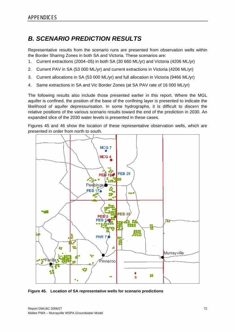
APPENDICES
Report DWLBC 2006/27 Mallee PWA – Murrayville WSPA Groundwater Model
72
B. SCENARIO PREDICTION RESULTS Representative results from the scenario runs are presented from observation wells within the Border Sharing Zones in both SA and Victoria. These scenarios are: 1. Current extractions (2004–05) in both SA (30 660 ML/yr) and Victoria (4206 ML/yr)
2. Current PAV in SA (53 000 ML/yr) and current extractions in Victoria (4206 ML/yr)
3. Current allocations in SA (53 000 ML/yr) and full allocation in Victoria (9466 ML/yr)
4. Same extractions in SA and Vic Border Zones (at SA PAV rate of 16 000 ML/yr)
The following results also include those presented earlier in this report. Where the MGL aquifer is confined, the position of the base of the confining layer is presented to indicate the likelihood of aquifer depressurisation. In some hydrographs, it is difficult to discern the relative positions of the various scenario results toward the end of the prediction in 2030. An expanded slice of the 2030 water levels is presented in these cases.
Figures 45 and 46 show the location of these representative observation wells, which are presented in order from north to south.
Figure 45. Location of SA representative wells for scenario predictions
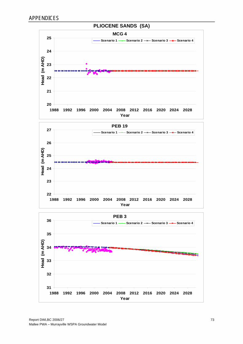
APPENDICES
Report DWLBC 2006/27 Mallee PWA – Murrayville WSPA Groundwater Model
73
PLIOCENE SANDS (SA) MCG 4
20
21
22
23
24
25
1988 1992 1996 2000 2004 2008 2012 2016 2020 2024 2028Year
Hea
d (m
AH
D)
Scenario 1 Scenario 2 Scenario 3 Scenario 4
PEB 19
22
23
24
25
26
27
1988 1992 1996 2000 2004 2008 2012 2016 2020 2024 2028Year
Hea
d (m
AH
D)
Scenario 1 Scenario 2 Scenario 3 Scenario 4
PEB 3
31
32
33
34
35
36
1988 1992 1996 2000 2004 2008 2012 2016 2020 2024 2028Year
Hea
d (m
AH
D)
Scenario 1 Scenario 2 Scenario 3 Scenario 4

APPENDICES
Report DWLBC 2006/27 Mallee PWA – Murrayville WSPA Groundwater Model
74
MURRAY GROUP (SA) MCG 7
10
15
20
25
30
1988 1992 1996 2000 2004 2008 2012 2016 2020 2024 2028Year
Hea
d (m
AH
D)
Scenario 1 Scenario 2 Scenario 3 Scenario 4
Base of confining layer -15m
PEB 25
0
10
20
30
1988 1992 1996 2000 2004 2008 2012 2016 2020 2024 2028Year
Hea
d (m
AH
D)
Scenario 1 Scenario 2 Scenario 3 Scenario 4
Base of confining layer -2m
PEB 17
5
10
15
20
25
30
35
1988 1992 1996 2000 2004 2008 2012 2016 2020 2024 2028Year
Hea
d (m
AH
D)
Scenario 1 Scenario 2 Scenario 3 Scenario 4
Base of confining layer -7m
2030

APPENDICES
Report DWLBC 2006/27 Mallee PWA – Murrayville WSPA Groundwater Model
75
PNR 7
22
27
32
37
42
1988 1992 1996 2000 2004 2008 2012 2016 2020 2024 2028Year
Hea
d (m
AH
D)
Scenario 1 Scenario 2 Scenario 3 Scenario 4
Base of confining layer 25m
RENMARK GROUP (SA)
PEB 35
35
36
37
38
39
40
1988 1992 1996 2000 2004 2008 2012 2016 2020 2024 2028Year
Hea
d (m
AH
D)
Scenario 1 Scenario 2 Scenario 3 Scenario 4
PEB 24
0
10
20
30
40
1988 1992 1996 2000 2004 2008 2012 2016 2020 2024 2028Year
Hea
d (m
AH
D)
Scenario 1 Scenario 2 Scenario 3 Scenario 4
Base of confining layer 6m
203
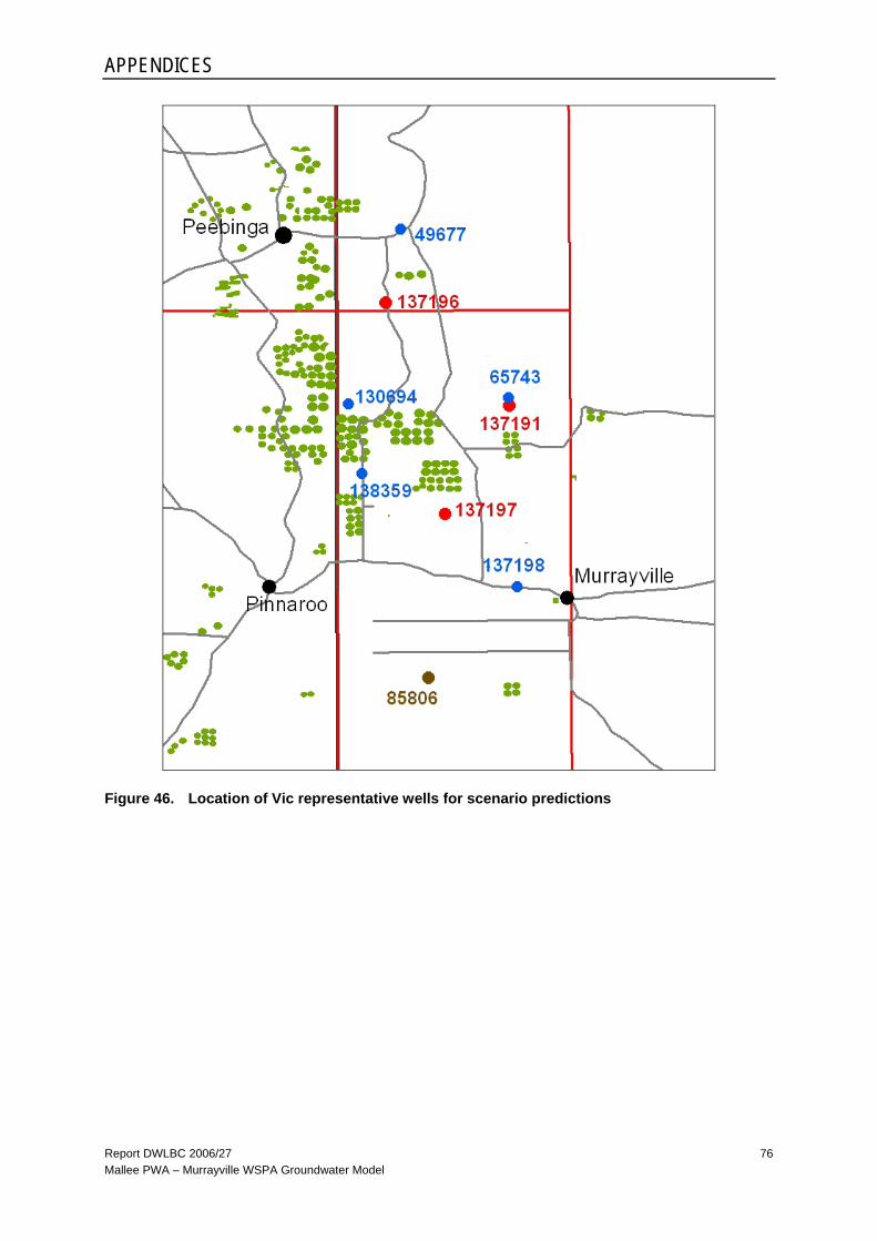
APPENDICES
Report DWLBC 2006/27 Mallee PWA – Murrayville WSPA Groundwater Model
76
Figure 46. Location of Vic representative wells for scenario predictions
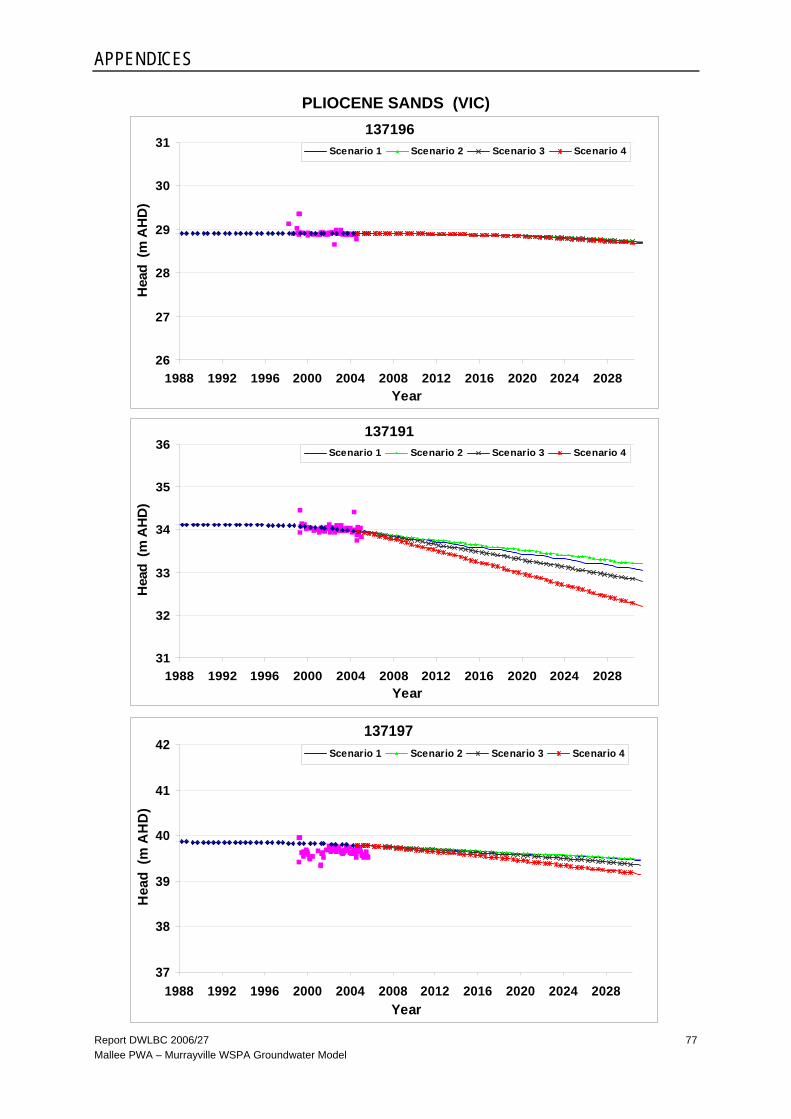
APPENDICES
Report DWLBC 2006/27 Mallee PWA – Murrayville WSPA Groundwater Model
77
PLIOCENE SANDS (VIC) 137196
26
27
28
29
30
31
1988 1992 1996 2000 2004 2008 2012 2016 2020 2024 2028Year
Hea
d (m
AH
D)
Scenario 1 Scenario 2 Scenario 3 Scenario 4
137191
31
32
33
34
35
36
1988 1992 1996 2000 2004 2008 2012 2016 2020 2024 2028Year
Hea
d (m
AH
D)
Scenario 1 Scenario 2 Scenario 3 Scenario 4
137197
37
38
39
40
41
42
1988 1992 1996 2000 2004 2008 2012 2016 2020 2024 2028Year
Hea
d (m
AH
D)
Scenario 1 Scenario 2 Scenario 3 Scenario 4
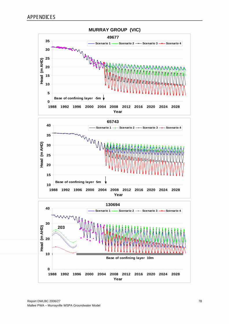
APPENDICES
Report DWLBC 2006/27 Mallee PWA – Murrayville WSPA Groundwater Model
78
MURRAY GROUP (VIC) 49677
0
5
10
15
20
25
30
35
1988 1992 1996 2000 2004 2008 2012 2016 2020 2024 2028Year
Hea
d (m
AH
D)
Scenario 1 Scenario 2 Scenario 3 Scenario 4
Base of confining layer -5m
65743
10
15
20
25
30
35
40
1988 1992 1996 2000 2004 2008 2012 2016 2020 2024 2028Year
Hea
d (m
AH
D)
Scenario 1 Scenario 2 Scenario 3 Scenario 4
Base of confining layer 5m
130694
0
10
20
30
40
1988 1992 1996 2000 2004 2008 2012 2016 2020 2024 2028Year
Hea
d (m
AH
D)
Scenario 1 Scenario 2 Scenario 3 Scenario 4
Base of confining layer 10m
203
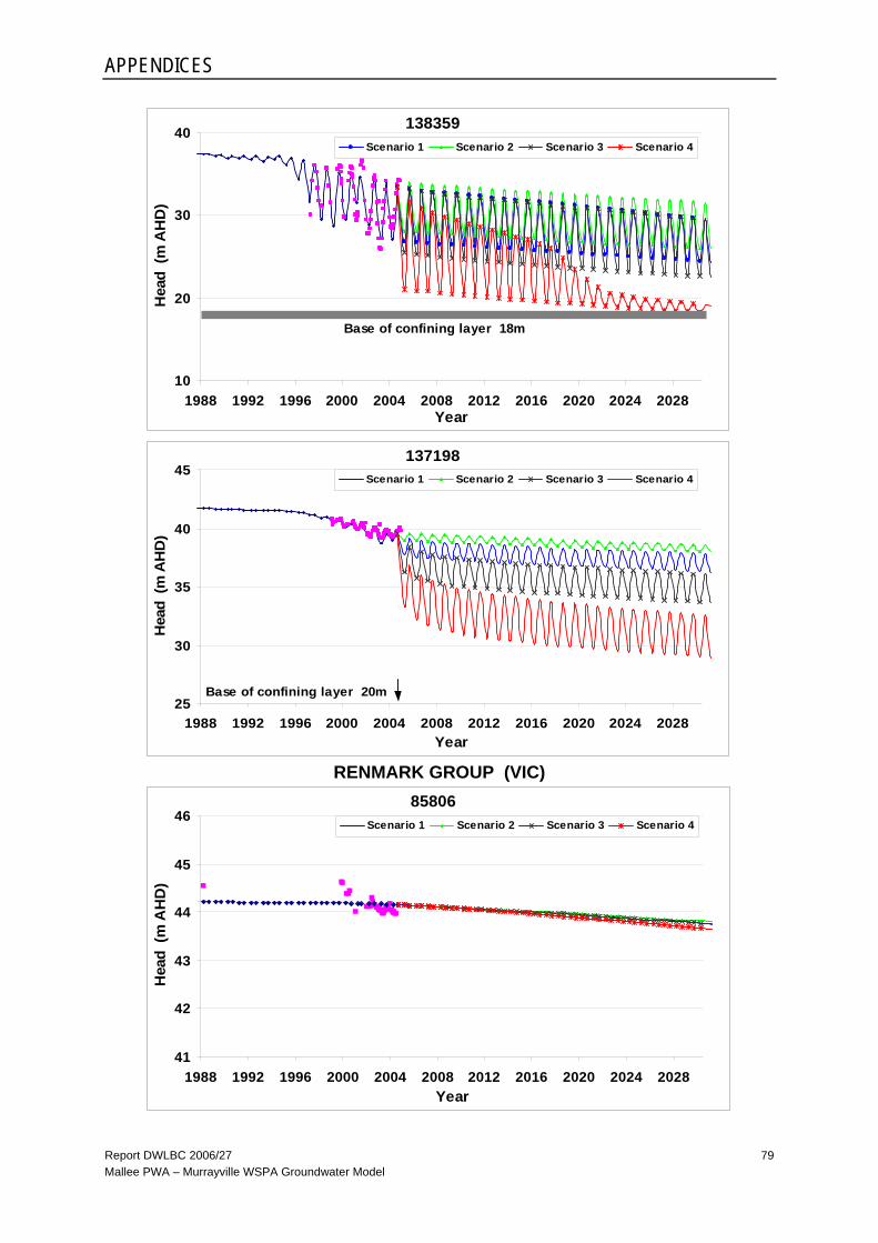
APPENDICES
Report DWLBC 2006/27 Mallee PWA – Murrayville WSPA Groundwater Model
79
138359
10
20
30
40
1988 1992 1996 2000 2004 2008 2012 2016 2020 2024 2028Year
Hea
d (m
AH
D)
Scenario 1 Scenario 2 Scenario 3 Scenario 4
Base of confining layer 18m
137198
25
30
35
40
45
1988 1992 1996 2000 2004 2008 2012 2016 2020 2024 2028Year
Hea
d (m
AH
D)
Scenario 1 Scenario 2 Scenario 3 Scenario 4
Base of confining layer 20m
RENMARK GROUP (VIC)
85806
41
42
43
44
45
46
1988 1992 1996 2000 2004 2008 2012 2016 2020 2024 2028Year
Hea
d (m
AH
D)
Scenario 1 Scenario 2 Scenario 3 Scenario 4
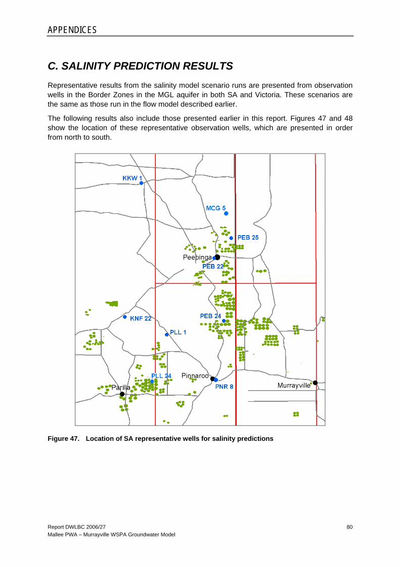
APPENDICES
Report DWLBC 2006/27 Mallee PWA – Murrayville WSPA Groundwater Model
80
C. SALINITY PREDICTION RESULTS Representative results from the salinity model scenario runs are presented from observation wells in the Border Zones in the MGL aquifer in both SA and Victoria. These scenarios are the same as those run in the flow model described earlier.
The following results also include those presented earlier in this report. Figures 47 and 48 show the location of these representative observation wells, which are presented in order from north to south.
Figure 47. Location of SA representative wells for salinity predictions
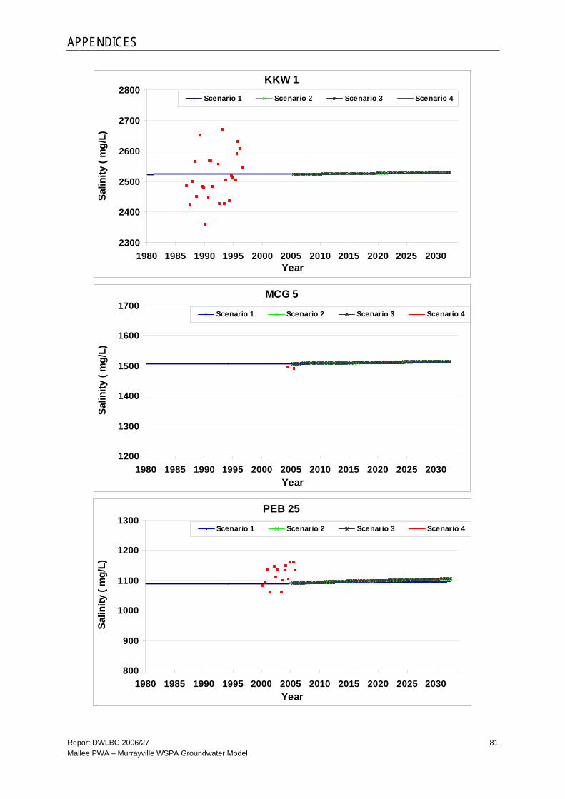
APPENDICES
Report DWLBC 2006/27 Mallee PWA – Murrayville WSPA Groundwater Model
81
KKW 1
2300
2400
2500
2600
2700
2800
1980 1985 1990 1995 2000 2005 2010 2015 2020 2025 2030Year
Salin
ity (
mg/
L)Scenario 1 Scenario 2 Scenario 3 Scenario 4
MCG 5
1200
1300
1400
1500
1600
1700
1980 1985 1990 1995 2000 2005 2010 2015 2020 2025 2030Year
Salin
ity (
mg/
L)
Scenario 1 Scenario 2 Scenario 3 Scenario 4
PEB 25
800
900
1000
1100
1200
1300
1980 1985 1990 1995 2000 2005 2010 2015 2020 2025 2030Year
Salin
ity (
mg/
L)
Scenario 1 Scenario 2 Scenario 3 Scenario 4
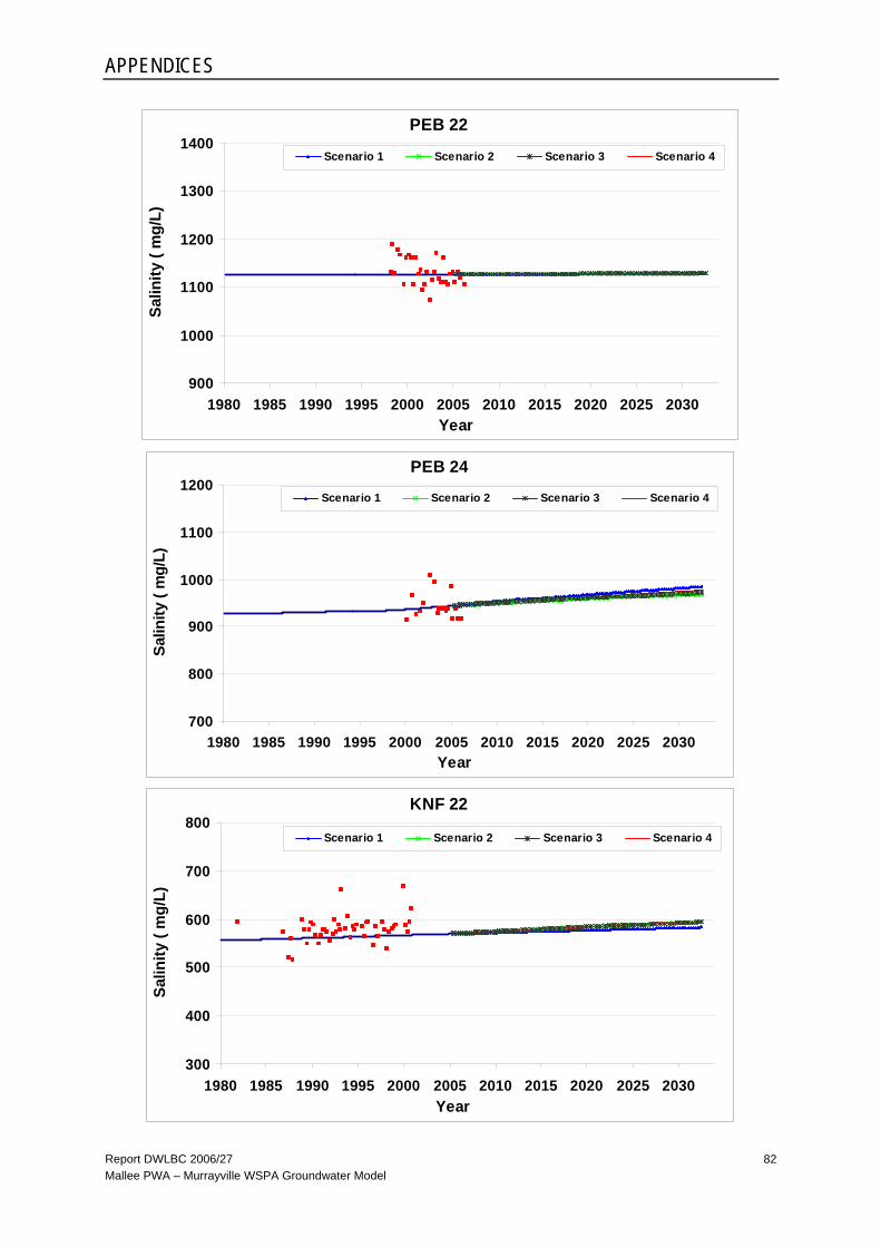
APPENDICES
Report DWLBC 2006/27 Mallee PWA – Murrayville WSPA Groundwater Model
82
PEB 22
900
1000
1100
1200
1300
1400
1980 1985 1990 1995 2000 2005 2010 2015 2020 2025 2030Year
Salin
ity (
mg/
L)Scenario 1 Scenario 2 Scenario 3 Scenario 4
PEB 24
700
800
900
1000
1100
1200
1980 1985 1990 1995 2000 2005 2010 2015 2020 2025 2030Year
Salin
ity (
mg/
L)
Scenario 1 Scenario 2 Scenario 3 Scenario 4
KNF 22
300
400
500
600
700
800
1980 1985 1990 1995 2000 2005 2010 2015 2020 2025 2030Year
Salin
ity (
mg/
L)
Scenario 1 Scenario 2 Scenario 3 Scenario 4

APPENDICES
Report DWLBC 2006/27 Mallee PWA – Murrayville WSPA Groundwater Model
83
PLL 1
2000
2200
2400
2600
2800
3000
1980 1985 1990 1995 2000 2005 2010 2015 2020 2025 2030Year
Salin
ity (
mg/
L)Scenario 1 Scenario 2 Scenario 3 Scenario 4
PLL 24
1000
1100
1200
1300
1400
1500
1980 1985 1990 1995 2000 2005 2010 2015 2020 2025 2030Year
Salin
ity (
mg/
L)
Scenario 1 Scenario 2 Scenario 3 Scenario 4
PNR 8
500
600
700
800
900
1000
1980 1985 1990 1995 2000 2005 2010 2015 2020 2025 2030Year
Salin
ity (
mg/
L)
Scenario 1 Scenario 2 Scenario 3 Scenario 4

APPENDICES
Report DWLBC 2006/27 Mallee PWA – Murrayville WSPA Groundwater Model
84
Figure 48. Location of Vic representative wells for salinity predictions
49679
500
1000
1500
2000
2500
3000
3500
4000
4500
1980 1985 1990 1995 2000 2005 2010 2015 2020 2025 2030Year
Salin
ity (
mg/
L)
Scenario 1 Scenario 2 Scenario 3 Scenario 4
The modelled salinity of 1000 mg/L for well 49679 is based on several nearby irrigation wells. The observed salinity reflects the probable shallower completion of the observation well.
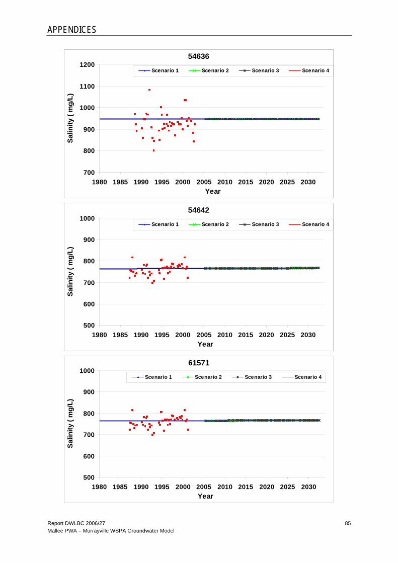
APPENDICES
Report DWLBC 2006/27 Mallee PWA – Murrayville WSPA Groundwater Model
85
54636
700
800
900
1000
1100
1200
1980 1985 1990 1995 2000 2005 2010 2015 2020 2025 2030Year
Salin
ity (
mg/
L)Scenario 1 Scenario 2 Scenario 3 Scenario 4
54642
500
600
700
800
900
1000
1980 1985 1990 1995 2000 2005 2010 2015 2020 2025 2030Year
Salin
ity (
mg/
L)
Scenario 1 Scenario 2 Scenario 3 Scenario 4
61571
500
600
700
800
900
1000
1980 1985 1990 1995 2000 2005 2010 2015 2020 2025 2030Year
Salin
ity (
mg/
L)
Scenario 1 Scenario 2 Scenario 3 Scenario 4
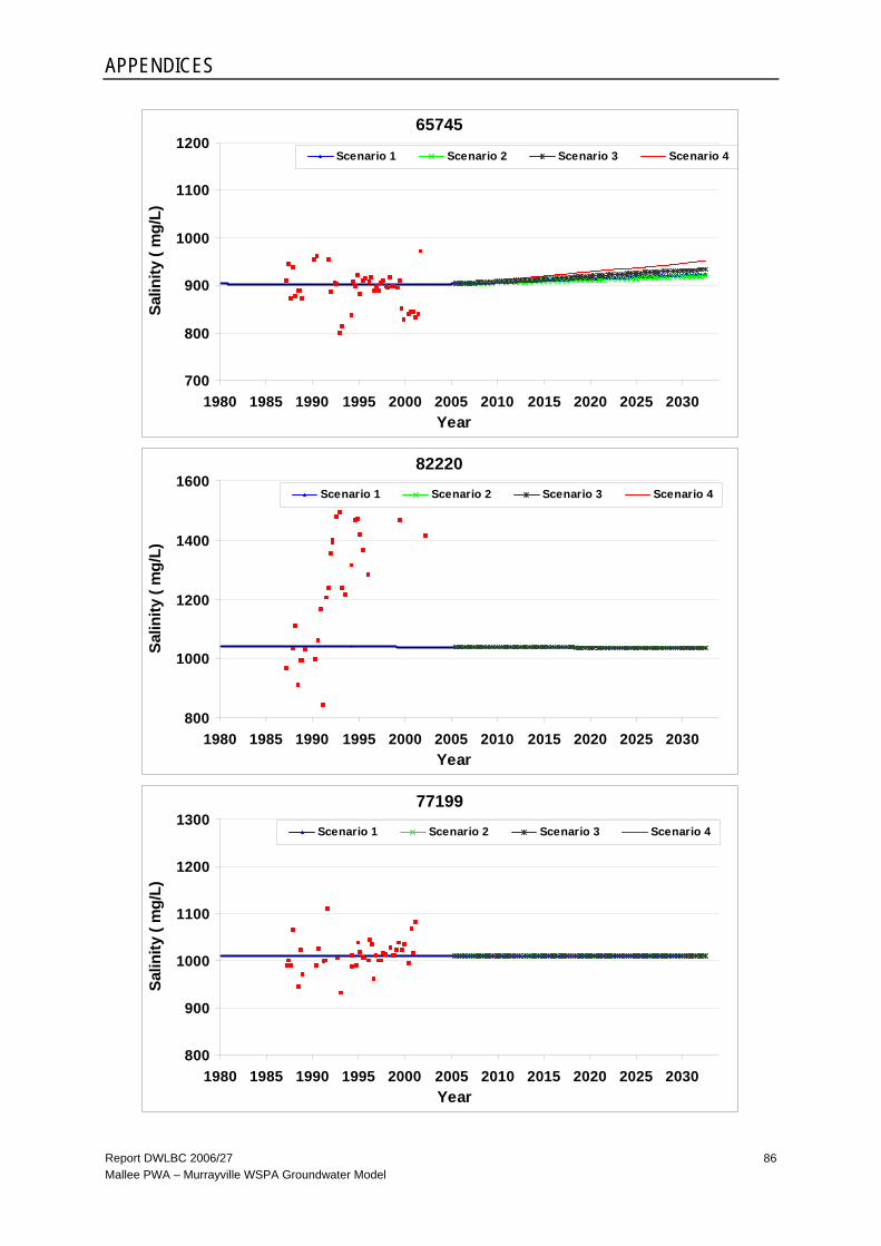
APPENDICES
Report DWLBC 2006/27 Mallee PWA – Murrayville WSPA Groundwater Model
86
65745
700
800
900
1000
1100
1200
1980 1985 1990 1995 2000 2005 2010 2015 2020 2025 2030Year
Salin
ity (
mg/
L)Scenario 1 Scenario 2 Scenario 3 Scenario 4
82220
800
1000
1200
1400
1600
1980 1985 1990 1995 2000 2005 2010 2015 2020 2025 2030Year
Salin
ity (
mg/
L)
Scenario 1 Scenario 2 Scenario 3 Scenario 4
77199
800
900
1000
1100
1200
1300
1980 1985 1990 1995 2000 2005 2010 2015 2020 2025 2030Year
Salin
ity (
mg/
L)
Scenario 1 Scenario 2 Scenario 3 Scenario 4

Report DWLBC 2006/27 Mallee PWA – Murrayville WSPA Groundwater Model
87
GLOSSARY Aquifer. An underground layer of rock or sediment which holds water and allows water to percolate through.
Aquifer, confined. Aquifer in which the upper surface is impervious and the water is held at greater than atmospheric pressure. Water in a penetrating well will rise above the top of the aquifer.
Aquifer test. A hydrological test performed on a well, aimed to increase the understanding of the aquifer properties, including any interference between wells, and to more accurately estimate the sustainable use of the water resource available for development from the well.
Aquifer, unconfined. Aquifer in which the upper surface has free connection to the ground surface and the water surface is at atmospheric pressure.
Aquitard. A layer in the geological profile that separates two aquifers and restricts the flow between them.
Calibration. The process by which the independent variables (parameters) of a numerical model are adjusted, within realistic limits, to produce the best match between simulated and observed data (usually water-level values). This process involves refining the model representation of the hydrogeologic framework, hydraulic properties, and boundary conditions to achieve the desired degree of correspondence between the model simulations and observations of the groundwater flow system.
Calibration, initial conditions. The initial hydrologic conditions for a flow system that are represented by its aquifer head distribution at some particular time corresponding to the antecedent hydrologic conditions in that system. Initial conditions provide a starting point for transient simulations.
Calibration, steady state. The calibration of a model to a set of hydrologic conditions that represent (approximately) an equilibrium condition, with no accounting for aquifer storage changes.
Calibration, transient or dynamic. The calibration of a model to hydrologic conditions that vary dynamically with time, including consideration of aquifer storage changes in the mathematical model.
Conceptual model. A simplified and idealised representation (usually graphical) of the physical hydrogeologic setting and our hydrogeological understanding of the essential flow processes of the system. This includes the identification and description of the geologic and hydrologic framework, media type, hydraulic properties, sources and sinks, and important aquifer flow and surface-groundwater interaction processes.
Heterogeneous. A medium which consists of different (non-uniform) characteristics in different locations.
Hydrograph. A graph that shows some property of groundwater or surface water (usually head or flow) as a function of time.
Permeability. A measure of the ease with which water flows through an aquifer or aquitard.
Potentiometric head. The potentiometric head or surface is the level to which water rises in a well due to water pressure in the aquifer.
Specific Yield. The ratio of the volume of water that a given mass of saturated soil or rock will yield by gravity to the volume of that mass.
Storage Coefficient (Storativity). The volume of water that a conductive unit will expel from storage per unit surface area per unit change in head. In a confined aquifer, it is computed as the product of specific storage and aquifer thickness. In an unconfined aquifer, it is equal to specific yield.

Report DWLBC 2006/27 Mallee PWA – Murrayville WSPA Groundwater Model
88
REFERENCES Anderson and Woessner, 1992. Applied groundwater modelling: Simulation of flow and advective transport, Academic Press Inc., Harcourt Brace Jovanovich Publishers, 381 p
ASTM, 1995. Standard Guide for Risk-Based Corrective Action Applied at Petroleum Release Sites. American society for Testing and materials, ASTM Designation E 17390095.
Barnett, S.R., 1983. Murray Basin hydrogeological investigation. Data assessment – Mallee region. South Australia Department of Mines and Energy. Report Book 83/18.
Barnett, S.R., 1990. Murray Basin hydrogeological investigation – Mallee Region groundwater modelling exercise. South Australia. Department of Mines and Energy. Report Book, 90/36.
Barnett, S.R., 2003. Mallee PWA and Murrayville WSPA - Groundwater Monitoring Status Report 2003. South Australia. Department of Water, Land and Biodiversity Conservation. DWLBC Report 2003/29.
Barnett, S.R., 2006. Mallee PWA and Murrayville WSPA - Groundwater Monitoring Status Report 2006. South Australia. Department of Water, Land and Biodiversity Conservation. DWLBC Report 2006/28.
Barnett, S.R. and Yan, W., 2000. Mallee Region groundwater modelling - Report No.1. South Australia. Department of Primary Industries and Resources. Report Book, 2000/00004.
Brown, C.M. and Stephenson, A.E., 1991. Geology of the Murray Basin, southeastern Australia. Bureau of Mineral Resources, Geology and Geophysics, Australia. Bulletin 235.
Cook, P.G., Walker, G.R. and Jolly, I.D., 1989. Spatial variability of groundwater recharge in a semiarid region. Journal of Hydrology, 111:195-212.
Lawrence, C.R., 1975. Geology, hydrodynamics and hydrochemistry of the souther Murray Basin. Geological Survey of Victoria, Memoir 30.
Leaney, F.W.J. and Herczeg, A.L., 1999. The origin of fresh groundwater in the SW Murray Basin and its potential for salinisation. CSIRO Division of Land and Water, Technical report, 7/99.
McDonald, M. G. and Harbaugh, A. W., 1988. A modular three-dimensional finite-difference groundwater flow model, Techniques of Water-Resources investigations, Book 6, chapter A1, United States Geological Survey.
Pickens, J. F., and Grisak, G. E., 1981. Modelling of scale-dependent dispersion in hydrogeologic system. Water Resources Research, vol 17(6): 1701 – 1711.
Sinclair Knight Merz, 2004. Murrayville groundwater quality data assessment and reporting - Reporting and analysis of groundwater sampling program for Wimmera Mallee Water.
Williams, A.F. 1976. Investigation of potential evaporation basins, Upper Murray, South Australia. Progress report No. 3. South Australia. Department of Mines and Energy. Report Book, 76/16.