May 2015

Working Paper Dyson School of Applied Economics and Management Cornell University, Ithaca, New York 14853-7801 USA

Management Areas and Fixed Costs in the Economics of Water Quality Trading

Tianli Zhao, Gregory L. Poe, and Richard N. Boisvert

It is the policy of Cornell University actively to support equality of educational

and employment opportunity. No person shall be denied admission to any

educational program or activity or be denied employment on the basis of any

legally prohibited discrimination involving, but not limited to, such factors as

race, color, creed, religion, national or ethnic origin, sex, age or handicap.

The University is committed to the maintenance of affirmative action

programs which will assure the continuation of such equality of opportunity.

Management Areas and Fixed Costs in the Economics of Water Quality Trading

By

Tianli Zhao1,2

Gregory L. Poe1 Richard N. Boisvert1

1. Dyson School of Applied Economics and Management, Cornell University2. Department of Economics, Cornell University

Abstract: Hung and Shaw’s (2005) trading-ratio system is modified to accommodate a management area approach wherein emissions sources are organized by impacts on identified “hot spots” and trading accounts for fixed as well as variable costs. An empirical example of phosphorus trading in a watershed with 22 potential traders demonstrates that marginal cost trading using a trading-ratio system yield nominal cost savings of less than 1% at the watershed level relative to the no-trade situation. A management area approach that accounts for fixed costs achieves over 13% in costs savings. The pattern of cost-effective trades is modeled using a mixed-integer approach.

Acknowledgements: This project was made possible through funding provided by the EPA Targeted Watershed Grant Program (WS972841) and USDA Hatch Project funds provided through Cornell University (121– 7822). Without implication, we appreciate helpful inputs into this and related research from Chris Obrupta, Josef Kardos, and Yukako Sado. Neither the EPA nor the USDA has reviewed or endorsed this article. The views expressed herein are those of the authors and may not reflect the views of these agencies.

2

Management Areas and Fixed Costs in the Economics of Water Quality Trading

An expanding body of evidence has demonstrated that, despite substantial federal, state and

local investments, nearly all active water quality trading programs are characterized by low

trading volumes and nominal cost savings at best (King and Kuch, 2003; King, 2005; Morgan

and Wolverton, 2005; Faeth, 2006; US EPA 2008; Selman et al. 2009; Fisher-Vanden and

Olmstead, 2013). While there are undoubtedly a number of institutional or behavioral factors

that inhibit water quality tradingi, we are motivated in this study by Hoag and Hughes-Popp’s

(1997) arguments that translating economic theory into practice may necessitate a reexamination

of the “…[m]ain principles associated with water pollution credit trading… to identify factors

that influence program feasibility” (p. 253). Using the empirical modeling results from a case

study of the Non-Tidal Passaic River Basin phosphorus emissions trading program, we focus in

this paper on two fundamental economic aspects of the disparity between the theory and the

practice of water quality trading programs.

First, recognizing that hydrological systems and Total Maximum Daily Load (TMDL)

objectives for a particular watershed may be quite complex, we broadly interpret Hung and

Shaw’s (2005) Trading Ratio System (TRS) to enable firms to trade allowances upstream and

across tributaries within a specified multi-zone management area. Hung and Shaw show that the

TRS can cost effectively meet water quality requirements at all points in a watershed through

trades that reallocate permits from upstream to downstream sources, each operating in a distinct

zone.ii,iii One can logically extend this structure to multiple dischargers in a zone by assuming

that dischargers have a one-to-one trading ratio within a zone. However, as Tietenberg (2006, p.

94) notes, “…other ratios potentially could provide policy makers with an additional degree of

freedom.” We investigate this possibility by modeling a “Management Area” (MA) policy

3

proposed for the Upper-Passaic River Basin TMDL (Obrupta et al., 2008).iv Rather than

restricting effluent concentration levels at all points within a watershed, the MA approach is

motivated by the actuality that TMDL regulations are often oriented toward avoiding critical

“hot spots” (i.e., localized areas with unacceptably high degraded water quality due to high

concentrations of a pollutant). The MA approach groups pollution sources with a common

endpoint at one of these hot spots, and may or may not have trading ratios equal to unity between

sources. Within an MA both upstream and downstream trades are permitted. Trading between

MAs is consistent with TRS-type trading rules wherein only downstream sales of allowances are

allowed.

Second we raise the practical concern that the canonical theoretical presentation of tradable

pollution allowances, in which firms buy and sell pollution allowances based on marginal

abatement costs relative to the market determined price, is inappropriate for cost-effectively

meeting a TMDL in a watershed in the long run. Such open-market exchange programs have

been effective in settings, such as the U.S. Acid Rain Trading program, that are characterized by

large numbers of potential traders with heterogeneous abatement technologies across firms, and

heterogeneous present capacity to meet standards (Schmalensee and Stavins, 2013). However,

as suggested by Sado et al. (2010), this type of a trading mechanism is less amenable to point-to-

point source water quality trading programs characterized by a small number of potential traders

in a watershed, with discrete and homogeneous abatement technologies across firms, and most, if

not all, firms lacking the present capacity to meet the specified standard. In such settings,

managers may be reluctant to not upgrade (and buy permits instead) or to develop excess

treatment capacity (and sell permits) because of the relative lack of buyers and sellers in a thin

4

market. Suter et al. (2013) support this conjecture empirically in an experimental economics

context.

We recognize that neither zonal aggregation nor capital cost considerations are novel issues

in the pollution trading literature. For example, Tietenberg (2006) provides a comprehensive

review of studies with various zonal configurations, mostly in the context of air quality, while

Bennett et al. (2000) examine the consequences of broadening trading areas with respect to the

Long Island Sound Nitrogen Credit Exchange program. Decades ago, Rose-Ackerman (1973)

and Kneese and Bower (1968) raised concerns about market incentives vis-à-vis substantial,

discrete fixed costs likely to arise in water quality treatment. Hanley et al. (1998), the US EPA

(2004), Caplan (2008), Sado et al. (2010), and Suter et al. (2013) have discussed the importance

of the discontinuous or stepwise nature of capital costs in the design and implementation of

water quality trading programs. Further, a series of least-cost abatement studies for sewage

treatment have included fixed costs in their identification of optimal watershed investment plans,

inferring substantial opportunities for gains from trade in water quality markets (David et al.,

1980; Eheart, 1980; Eheart et al., 1980; Bennett et al., 2000).

These empirical studies, however, have failed to identify optimal trading patterns between

firms that explicitly take advantage of fixed cost savings. Rather, they typically assert that firms

with above (below) average incremental costs will be buyers (sellers), and they have been

constructed largely within a single receptor framework. For example, David et al. (1980, p. 268)

trace out an aggregate least-cost phosphorus removal curve, identify the industry marginal cost

of removing the unit of effluent that just meets the prescribed standard, and infer that firms with

unit costs above this value will be demanders for allowances while dischargers with removal

costs below this value will be suppliers. More recently Bennett et al. (2000) similarly trace out

5

the least-cost abatement curve including fixed costs and identify total potential cost savings from

firms; but they do not model the pattern of trades that will occur between firms. Our contribution

in this paper is to directly model the trades across firms to explore empirically those factors that

could improve the cost-effectiveness of trading programs and enhance the economic viability of

water quality trading. In a case study, we demonstrate empirically that potential watershed-wide

costs savings can increase dramatically by relaxing zonal trading constraints and incorporating

fixed as well as variable costs into the determination of trading patterns.

The remainder of the paper begins with a section that provides background information on

the TMDL and the Upper-Passaic River Basin. We then introduce our conceptual framework,

using Hung and Shaw’s TRS model as a starting point. Applying this framework, we employ a

mixed-integer programming method to explore the effects of zonal aggregation and the cost-

savings associated with considering fixed and variable costs in the determination of a trading

regime. The final section concludes with a discussion of the need to explore long term contracts

in greater depth and/or to examine other incentives to encourage trading in the face of fixed

capital investments.

Essential Features of the Non-tidal Passaic River Watershed

The Non-Tidal or Upper Passaic River watershed is located primarily in northeastern New

Jersey, with the uppermost portion extending into New York State. This 803 square mile

watershed consists of the Passaic River and its tributaries, draining five densely populated

counties in New Jersey near the New York City Metropolitan area. Approximately one-quarter of

New Jersey’s population (i.e., two million people) resides within the watershed boundaries. It is

a major source of drinking water both inside and out of the basin.

6

As shown in Figure 1 the Passaic River initially flows south, then turns and flows in a north-

easterly direction, and then turns east and finally south before reaching Newark Bay. The formal

terminus of the Upper Passaic River is Dundee Dam, which separates the Upper, Non-Tidal

Passaic River (P) from the tidal part of the Passaic River. The Dead River (D) joins the Passaic at

the point where it first changes direction. At the watershed’s center, the Rockaway River (R)

flows into the Whippany River (W), and in turn, the Whippany River flows into the Passaic. The

Wanaque River (WQ) begins in the northern part of the watershed, flowing into the Pompton

River (T), which subsequently joins the Passaic. Below this confluence, but above the Dundee

Dam, the Singac Brook and the Peckman River join the Passaic River.

In April 2008, a final TMDL rule was promulgated for this river basin (NJDEP, 2008),

calling for more than an 80% reduction in the total phosphorus concentration emissions from 22

Waste Water Treatment Plants (WWTPs) in the watershed. The TMDL specifies the following:

“Except as necessary to satisfy the more stringent criteria…or where watershed or site-specific criteria are developed…phosphorus as total P shall not exceed 0.1 [mg/l] in any stream, unless it can be demonstrated that total P is not a limiting nutrient and will not otherwise render the waters unsuitable for the designated uses.” (NJDEP, p. 15)

The 22 WWTPs are depicted in Figure 1 and the corresponding pre-TMDL flow and

concentration levels are provided in the first five columns of Table 1. The 0.1 mg/l concentration

level indicated in the TMDL language above translates into a long-term (i.e. annual) average 0.4

mg/l effluent from each of the 22 dischargers. Prior to the TMDL rule, the average (flow

weighted) total phosphorus emissions across WWTPs were estimated to be 2.13 mg/l.

The Modeling Framework

We begin this section with the development of the Hung and Shaw (2005) trading ratio system

for water quality trading in which permits can only be sold from upstream sellers to downstream

7

buyers and prices are based on differential marginal costs of treatment. We then develop a

second model where, because of the specific hydrology of the watershed, it is appropriate to

define management areas that group pollution sources with a common endpoint at a discrete hot

spot. Finally, we develop a third model that accommodates the cost of investing in new

abatement technology as well as the variable costs of treatment.

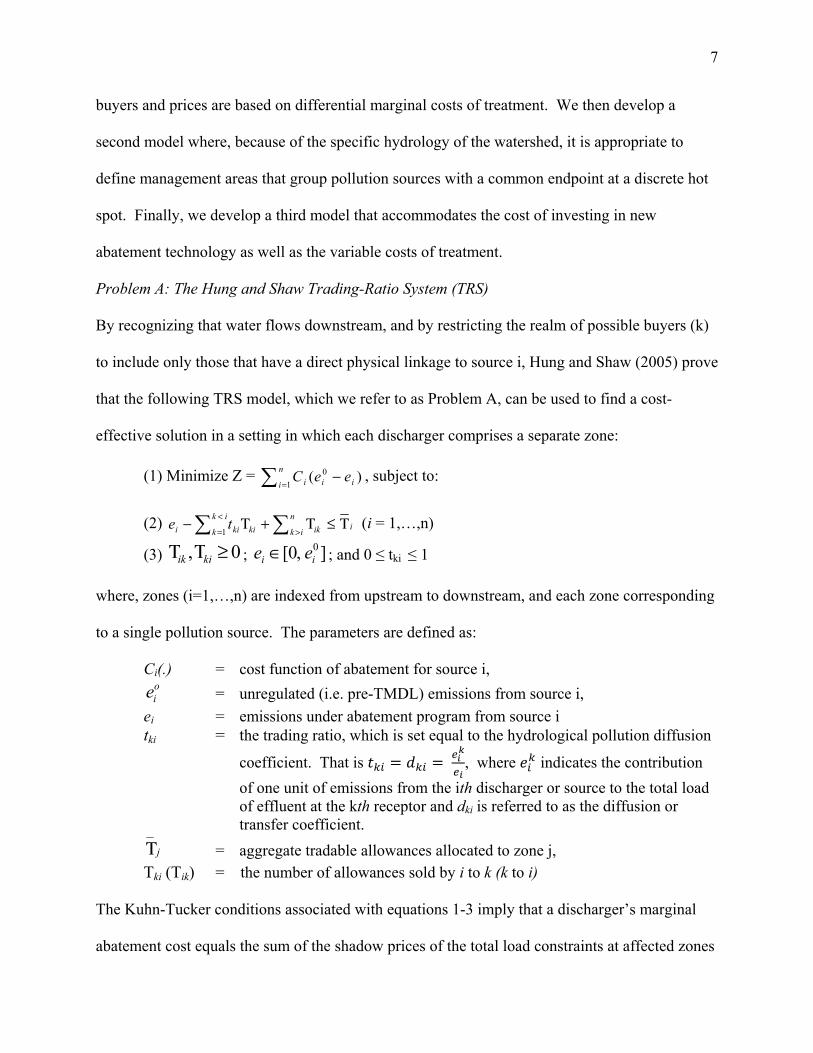
Problem A: The Hung and Shaw Trading-Ratio System (TRS)

By recognizing that water flows downstream, and by restricting the realm of possible buyers (k)

to include only those that have a direct physical linkage to source i, Hung and Shaw (2005) prove

that the following TRS model, which we refer to as Problem A, can be used to find a cost-

effective solution in a setting in which each discharger comprises a separate zone:

(1) Minimize Z = =−n

i iii eeC1

0 )( , subject to:

(2) >

<

=Τ≤Τ+Τ− n

ik iikik

k kikii te1

(i = 1,…,n)

(3) 0, ≥ΤΤ kiik ; ],0[ 0ii ee ∈ ; and 0 ≤ tki ≤ 1

where, zones (i=1,…,n) are indexed from upstream to downstream, and each zone corresponding

to a single pollution source. The parameters are defined as:

Ci(.) = cost function of abatement for source i, oie = unregulated (i.e. pre-TMDL) emissions from source i,

ei = emissions under abatement program from source i tki = the trading ratio, which is set equal to the hydrological pollution diffusion

coefficient. That is = = , where indicates the contribution of one unit of emissions from the ith discharger or source to the total load of effluent at the kth receptor and dki is referred to as the diffusion or transfer coefficient.

jΤ = aggregate tradable allowances allocated to zone j, Tki (Tik) = the number of allowances sold by i to k (k to i)

The Kuhn-Tucker conditions associated with equations 1-3 imply that a discharger’s marginal

abatement cost equals the sum of the shadow prices of the total load constraints at affected zones

8

weighted by transfer coefficients (Hung and Shaw, 2005) and that least-cost trading between

individual sources i and k with respect to a common downstream receptor achieves the spatially

adjusted equimarginal relationship associated with the least-cost abatement,

(4) )()(1)(1)( j

kkk

kk

kji

ii

ij

jii eMC

eeC

deeC

deMC =

∂∂=

∂∂= .

In the special case when k=j, then dkj = 1. When k and j are not directly connected

hydrologically, then dkj = 0.

Management Areas (MA) Approach: We extend Hung and Shaw’s TRS model to more closely

represent the MA approach being applied to phosphorus trading in the Non-Tidal Passaic River

Basin. As a reference point, the typical conceptualization of a multi-zone system treats

emissions from various sources within a zone as having equal effects on water quality

(Tietenberg, 2006). Hung and Shaw adopt this formulation, defining a trading zone “as an area

in which the environmental effects of the effluent of a particular pollutant are the same” (p. 99).

Within this framework, the trading ratios between sources within a zone would be set to unity.

With respect to the Non-Tidal Passaic River Basin TMDL, the 0.1 mg/l restriction on total

phosphorus was found to be overly restrictive for most of the watershed (Obropta et al., 2008). In

accordance with the TMDL language quoted above, the maximum ambient concentration level

of 0.1 mg/L could be relaxed at all but two locations in the watershed: the area near the

confluence of the Passaic and Pompton Rivers, and at Dundee Dam. Put differently, by meeting

the water quality constraints at these critical junctures, one could avoid any hotspots at other

points in the watershed.

Based on this hydrological modeling, three MAs are identified in the Upper Passaic River

Basin TMDL (Obrupta et al., 2008): the Upper Passaic MA consisting of WWTPs D1-D3, P1-

P8, W1-W4, and R1 with associated downstream endpoint on the Passaic River immediately

9

below the confluence of the Passaic and Pompton rivers; the Pompton MA (WQ, T1 and T2)

with a downstream outlet at the endpoint of the Pompton River where it feeds into the Passaic

River; and the Lower Passaic MA, P9-P11, with endpoint at the Dundee Lake and Dam.

Accounting for a number of factors, including seasonal variations in flows, the MAs and the

patterns of allowable inter-MA trades are depicted schematically in the Figure 2. Allowable

trades between MAs include: 1) downstream trades from the Upper Passaic and Pompton MAs to

the Lower Passaic MA; and 2) cross-tributary trades from the Pompton MA to the Upper Passaic

MA, but not vice versa. While we refer to option two as a cross-tributary trade, such transactions

are only possible in the MA approach we outline below because the endpoint of the Upper

Passaic MA lies hydrologically below the endpoint of the Pompton MA as depicted

schematically in Figure 2. Within each MA, upstream and downstream trades are permitted

subject to the constraint that emissions within the MA do not exceed the water quality constraint

at the MA endpoint.

A series of trade scenarios were simulated to investigate if the proposed management area

framework would protect water quality and ensure the avoidance of hot-spots at the TMDL end

points. (Omni Environmental Coroporation, 2007). As discussed in Obrupta et al. (2008),

“…intramanagement and intermanagement area trade scenarios that would most stress the

system and simulate critical conditions were developed to test the proposed framework…. These

simulation results verify that the trading framework is robust and can be expected to protect

water quality” (p. 954).

Problem B: A Trading-Ratio-System for Management Areas

As discussed above, the way each MA is delineated guarantees that the endpoint for each MA is

the sole outlet of its MA, making it possible to separate each MA hydrologically. In other words,

10

as long as the water quality at the critical location is ensured, any allowance trading within any

MA would not jeopardize the water quality in other MAs. For this reason, the trading ratios for

intra-MA trading are designed to adequately protect the water quality at its end-point.

Specifically, let 1k and 2k be two sources within the management area K (i.e. Kkk ∈21, ).

Suppose k1 sells an allowance to k2, then k1 has to discharge 1keΔ units less, while k2 can

discharge 2keΔ units more. The following relationship determines the magnitude of

2keΔ needed to ensure that this trade has zero net effect at the MA end-point [K] :

(5) 0][][][ 2211

=⋅Δ+⋅Δ=Δ KkkKkkK dedee

Rearranging, we have the following trading ratio:

(6) ][

][

2

1

1

2

21Kk

Kk

k

kkk d

dee

t =ΔΔ

−= ,

which ensures that allowing both upstream and downstream trades within an MA will not affect

the water quality at its outlet [K]; however, other areas within the same MA might have elevated

concentrations as a result of trading. Because we have placed no restrictions on the relative

location of 1k and 2k in K , the trading ratio need not have an upper bound of unity. Moreover,

the definition of the MA precludes the possibility that these elevated concentrations will

engender a hot spot. One can thus regard the trading system within each MA as a bare-bones

version of the ambient permit system in which the problem of transaction complexity is avoided.

Appendix 1 provides a proof that setting intra-MA trading-ratios in this manner supports the

cost-effective allocation of allowances subject to water quality constraints at the MA end-points.

11

In a similar fashion, the trading ratios for inter-MA trades are designed to preserve the water

quality at each MA endpoint. Since only the buyer's endpoint is subject to the negative impact of

the trades, it is adequate simply to ensure the water quality endpoint of the buyer's MA.

Formally, let j be the seller and k be the buyer from different management areas J and K

respectively ( KkJj ∈∈ , ), where the outlet of J ([J]) is hydrologically upstream from the

outlet of K. Using the above notation for changes in emissions, the following equation

guarantees that the trade has zero net effects at the buyer's end-point [K]:

(7) 0][][ =⋅Δ+⋅Δ KkkKjj dede .

By rearranging, we have:

(8) ][

][

Kk

Kj

j

kjk d

deet =

ΔΔ−=

By comparing equation (8) with equation (6), we see that the trading ratio for both intra-M.A

trades and inter-MA trades are described by the same simple relation------the trading ratio is

equal to the relative diffusion rate to the end-point of the buyer's MA. One difference between

the two ratios is that equation (8) is bounded between zero and unity, while the trading ratio in

equation (6) is only restricted to be non-negative.

To gain further insight into the process of trades between upstream and downstream

MAs, the upstream end-point [J] can serve as an intermediary to which one can then apply a

multiplicative effect over diffusion from j to [K]. That is:

(9) ]][[][][ KJJjKj ddd ⋅=

Substituting equation (9) into equation (7) yields:

(10) 0][]][[][ =⋅Δ+⋅⋅Δ KkkKJJjj dedde

12

Since ][][ JjjJ dee ⋅Δ=Δ and ][][ KkkK dee ⋅Δ=Δ , equation (10) can be reduced to:

(11) 0][]][[][ =Δ+⋅Δ KKJJ ede

Finally, the equivalent trading ratio ]][[ KJt between the two end-points [J], [K] can be

determined by combining equations (8) and (11):

(12) ]][[][

][]][[ KJ

J

KKJ d

ee

t =ΔΔ

−=,

which is essentially the Hung and Shaw (2005) TRS result. Equation (12) demonstrates that the

inter-MA trading between two sources j and k is as if the two MA end-points [J] and [K] were

trading the "effective allowances" under the TRS-----the trading ratio equals the natural diffusion

rate between the two end-points. This result can be further interpreted as if there were an

imaginary broker at each MA end-point who buys (sells) allowances from (to) other brokers

following the TRS and sells (buys) them to (from) the sources within its MA. In other words,

one can think of the inter-MA trading as being carried out in two steps: allowances are traded

across MAs by "brokers" at each MA end-point under TRS, and then they are localized to each

source through intra-MA trading.

Hung and Shaw's (2005) TRS guarantees that, in the first step, effective allowances can be

traded between MA end-points in a cost-effective manner, while also meeting the environmental

quality at all end-points. Since the cost-effectiveness of the second step--trading within an MA--

has been demonstrated, the entire MA trading process is consummated in a cost-effective

manner subject to the environmental standard at all MA end-points.v

By incorporating the MA approach, the trading model is now re-written as Problem B:

(1’) Minimize Z = =−n

i iii eeC1

0 )( , subject to:

13

(2’) in

k ikkin

kIi

Iki d

de Τ≤Τ+Τ− == 11

][

][ (i = 1,…,n)

(3’) 0, ≥ΤΤ kiik ; and ],0[ 0ii ee ∈ .

While not explicit in the above equations, the definition of dki implies that di[I] > 0 and dk[I] ≥ 0,

restricting the ratio in equation (2’) to be non-negative. Because there is no upper bound

restriction on the ratio dk[I]/di[I] when k and i both lie in management area I, the trading equation

(2’) now allows intra-management area trades to take place in both directions.

To sum up, we have interpreted the Hung and Shaw (2005) TRS broadly to enable firms

to trade allowances upstream and across tributaries within a specified multi-discharger MA. By

aggregating firms with non-unitary exchange rates into MAs that focus on meeting

environmental objectives at specific endpoints and adopting a TRS system between MAs, we can

achieve cost-effective solutions for predetermined environmental standards at those end points.

Put somewhat differently, this aggregation of dischargers into an MA is analogous to the

“representative agent” alluded to by Hung and Shaw (see footnote 1). This MA approach has

particular merit in that the environmental authority can have the flexibility to choose exactly

which locations are to be protected while at the same time ensuring the cost-effectiveness of the

strategy. By way of comparison, control authorities in a typical zonal approach with a one-to-

one trading ratio within a zone would have to increase the amount of required reductions in

emissions for the entire watershed to create a margin of safety for the critical locations. This

requirement would defeat a central purpose of zonal permit approaches--the prevention of over-

control (Tietenberg, 2006).

Problem C: Discrete Capital Costs

Our second extension of the TRS model is to account for discrete, fixed capital costs associated

with upgrading abatement capacity to enable plants to treat effluent to a lower concentration

14

level. While the addition of chemicals or other small changes can facilitate additional abatement

control in some instances, there are likely to be limits to such opportunities for any initial capital

configurations at the plants.

“Generally, pollution controls are feasible to implement in relatively large installments that [can] reduce multiple units of pollutants. Point sources in particular tend to purchase additional loading reduction capability in large increments” (US EPA, 1996, p. 3-2).

The following cost minimization problem (Problem C) explicitly considers the allocation of

fixed capital investment as well as variable costs in identifying the optimal abatement decisions

among dischargers. The model is given by:

(1’’) min = =−n

i iioii xeeCZ 1

),( = ])()([1 =

+n

i iiixi xCCeOM i subject to:

(2’’) i

n

k ikkin

kIi

Iki d

de Τ≤Τ+Τ− == 11

][

][ ( i = 1, ..., n)

(3’’) 0)( iiii eex ≤≤φ ; kiΤ , 0≥Τik and ii Zx ∈ ( i = 1, ..., n )

where the total annual abatement cost ),( iioii xeeC − is determined by continuous variable ie

and discrete integer variable xi. On the right hand side of equation (3’’), )( ixi eOM i denotes the

annual operating and management costs of firm i with investment level xi, at final effluent level

ie , and )( ii xCC denotes the annualized capital cost of firm i when it upgrades the capacity to

the level xi. We use xi as a superscript on the annual OM cost function because the facility

upgrade for a firm may also affect its variable cost function.

We also assume that the maximal abatement capacity of each firm is determined by its

own facility upgrade level, ii Zx ∈ . Hence, each firm's maximal achievable level of abatement is

bounded by a function of its upgrade level xi : )( iii xe φ≥ . Since each integer set Zi may be

different, each firm may face a different spectrum of upgrade choices. In addition, since the

15

capital investments are assumed irreversible, each firm can only upgrade but never downgrade its

capacity to abate. Consequently, if firm i has a certain level of existing capacity to remove the

pollutant, then "0" must not be in its choice set Zi

The nature of the solutions to this model are evident from the Kuhn-Tucker conditions of the

standard convex programming model that are associated with a specific branch of the integer

model in which each firm’s upgrade level is fixed (Zhao, 2013). Based on these conditions (see

Appendix 2) the characteristics of these solutions are summarized into the following six facts:

i. For a discharger operating at an interior point, willingness to pay (WTP) and willingness

to sell (WTS) are unique, both equaling the marginal cost of abatement.

ii. For a discharger constrained by eio, excess allowances will be sold at any positive price.

In other words, this discharger’s WTS is NOT unique. On the other hand, this discharger’s

WTP is trivial because it is not allowed to increase its effluent any further.

iii. For a discharger operating at the maximum physical capacity to abate, )( ii xφ , WTP is

bounded by a lower bound of marginal abatement cost and an arbitrarily determined high

price as the upper bound determined by the level of the penalty for non-compliance.

iv. Trade between any pair of the “interior” dischargers has a unique price ratio which

follows i

kkit

λλ

= , where λ is the shadow price.

v. Trade between an “interior” discharger and a “corner” discharger does not have a

unique price ratio, while it is bound above (below) by on the “interior” discharger's WTP

(or WTS).

vi. Trade between any pair of the “corner” dischargers does NOT have a unique price ratio,

the actual trading price of permits depends on bargaining.

Altogether these six results suggest that a unique price between dischargers will emerge only

when both dischargers are operating at an interior solution. When either of the dischargers is

operating at a corner solution, the permit price is not unique, and hence will require a bargaining

outcome. We return to this practical issue below.

16

The Data and the Empirical Specification

There are three essential components of the data needed to estimate total abatement costs and

trade patterns: 1) data for the initial effluent allowed for each WWTP under the TMDL; 2) the

transfer coefficients or trading ratios between each plant for which trading is possible; and 3)

data for OM and capital costs of phosphorus abatement for each WWTP.

The Environmental Capacity and the TMDLs

Under the baseline, no-trade policy, the allowable firm (or zonal) discharges are specified under

each discharger’s National Pollution Discharge Elimination System (NPDES) permits to not

exceed 0.40 mg/l total phosphorus (P), calculated as a long-term (i.e. annual) average (NJDEP,

2008). As depicted in the first five columns of Table 1, the current phosphorus effluent levels

differ substantially among plants, with only two WWTPs presently capable of meeting the 0.40

mg/l standard (also see the 13th column). The average pre-TMDL phosphorus concentration was

2.13 mg/l, well above the TMDL’s target effluent level of 0.40 mg/l.

The Trading Ratios:

The transfer coefficients and trading ratios are based on several scientific factors such as the rate

of inflow-outflow of pollutants, the bio-physical conditions, and the geography of the designated

areas. The transfer coefficients were derived by the distance between the outlet of the point

source and the target location, the settling and uptake rates of orthophosphate and organic

phosphorus occurring in the flow path, and the ratio of orthophosphate and organic phosphorus

discharged from the source (Najarian Associates, 2005). Because trading ratios varied across

probabilistic water level scenarios, each trading ratio represents the worst-case scenario--the

most vulnerable condition for a each buyer-seller pair across three distinct water level scenarios.

Table 2 contains the resulting trading-ratio matrix corresponding to the One-Discharger-

17

Per-Zone TRS model (Problem A). Empty cells indicate that emissions from potential sellers do

not have a direct effect on water quality at the buyer’s location. Consistent with the downstream

trading structure of the Hung and Shaw TRS system, trading ratios are bounded by zero and one

and all feasible trades lie above the main diagonal.

Trading ratios corresponding to the management area approach characterized in Problems

B and C and Figure 2 are provided in Table 3. In contrast to Table 2, trading opportunities

appear both above and below the main diagonal, indicating the possibility for both downstream

and upstream trades for some buyer/seller combinations. The elements of the matrix are not

symmetrical in the sense that the trading ratio for the transfer of a permit between a buyer and a

seller is not necessarily the inverse of the trading ratio if the direction of trade were reversed. For

example, P8 would be allowed to increase its phosphorus emissions by 0.714 lbs. for each pound

of allowances purchased from R1. However, R1 could only increase phosphorus emissions by

1.235 lbs., which is less than . = 1.401, for each pound of allowance purchased from P8. In

this case, the product of the two ratios equals 0.88 (1.235 * 0.714) < 1, thus preluding the

possibility of profitable circular trading. This relationship generalizes to the entire matrix such

that tik * tki ≤ 1 ∀ i,k. because the worst-case trading ratios, as discussed above, are utilized.

Estimating the Costs of Phosphorus Abatement

Since most WWTPs in the watershed currently have little or no present capacity to remove

phosphorus, we estimate consistent phosphorus removal cost functions for both yearly OM and

capital costs from data for the actual costs of 104 treatment plants located in the Chesapeake Bay

watershed (NRTCTF 2002) and from an engineering study conducted in Georgia (Jiang et al.

2005). For the 104 Chesapeake Bay waste water treatment plants, we have data on daily flow

and annual Operating and Management (O&M) and cost for several effluent concentrations (e.g.

18

2mg/l; 1mg/l; 0.5mg/l; and 0.1mg/l). The following specification is estimated for O&M costs.

012111098

7654321

lnlnlnlnlnlnlnlnlnlnlnln&ln

uFCRFRCRRFCTFTCTTFCFCMO

+⋅⋅+⋅+⋅++⋅⋅+⋅+⋅++⋅+++=

αααααααααααα

where C is final phosphorus concentration in mg/l; F is daily flow in million gallons per day; T is

a binary technology variable equaling 1 (0) if biological (chemical) treatment is used; and R is a

regional indicator of whether the observations was drawn from the Georgia (R=1) or Chesapeake

(R=0) studies. Given this specification, the following cost function is estimated using OLS, with

Huber-White corrections to the covariance matrix to account for the clustering of multiple

observations per WWTP:

(13) 95.0lnln050.0180.1ln314.0

650.0lnln046.0ln796.0ln990.0876.9&ln2

*)020.0(**)179.0(**)022.0(

**)083.0(**)014.0(**)030.0(**)020.0(**)058.0(

=⋅⋅−+⋅+

+⋅++−=

RFCGGCT

TFCFCMO

The numbers in parentheses are estimated standard errors with “*”, and “**” indicating

significance at the 5% and 1% levels, respectively. Variables were retained in the final

estimated equation only if the estimated p values for the coefficients were less than 0.20.

Using a similar regression strategy, the following capital investment cost (CC) function is

estimated:

(14) 97.0680.0lnln114.0ln290.0ln442.0

996.0lnln128.0ln347.0ln985.0889.11ln2

)368.0(**)031.0(**)038.0(**)044.0(

**)230.0(**)031.0(**)041.0(**)010.0(**)011.0(

=+⋅⋅+⋅+⋅+

+⋅−+−=

RRFCTFTCT

TFCFCCC

Given geographic proximity and other similarities between the Chesapeake Bay and Passaic

watersheds, the Chesapeake data are thought to provide the preferred baseline for our analyses.

To accomplish this, the regional dummy R is set equal to "0" for the 22 firms in the Passaic

watershed. Further, the data from the Chesapeake Bay study are for inexpensive chemical

removal of phosphorus, and we assume this technology is adopted by the Passaic WWTPs with

19

no current capacity to treat phosphorus. For the three plants (W1, W2 and R1) that operate

biological phosphorus removal processes, we adjust the coefficients by setting T=1.

The elasticities of both O&M cost and Capital cost can be derived by taking the

logarithmic partial derivatives of above equations with respect to concentration level (see Zhao,

2013). The results can be summarized as: 1) For the range of flows in this study the elasticities

for both O&M cost and Capital costs are negative, indicating that as the final concentration goes

down, both costs rise; (2) O&M costs are more elastic for smaller plants (with lower discharge

flow) than for larger plants; and (3) The capital costs required to retrofit facilities are more

elastic for larger plants. These properties conform to the basic economic intuition as well as

common sense. In addition, the coefficients for the biological plants shift the cost functions

upward but, at the same time, the cost elasticities with respect to concentration decline. These

differences are consistent with the results from the Georgia study. Relative to chemical

abatement, biological removal processes generally involve higher operating costs and are more

investment intensive; they are, however, more efficient in phosphorus abatement to low

concentration levels.

Following Sado et al. (2010), we generate a discrete capital cost function by allowing for five

discrete concentrations: (1) current level > target concentration > 1.0 mg/l; (2) 1.0 mg/l > target

concentration > 0.50 mg/l; (3) 0.50 mg/l > target concentration > 0.25 mg/l; (4) 0.25 mg/l >

target concentration > 0.10 mg/l; and (5) 0.10 mg/l > target concentration. The corresponding

capital costs for each WWTP and treatment level are provided in Table 1, columns 7-12.

Although informed by engineers, these discrete capital cost thresholds are arbitrary.

20

General Trading Patterns and Cost Savings under Alternative Trading Scenarios

This section identifies the cost-effective abatement levels for each WWTP, the resulting patterns

of trade between WWTPs, and the cost savings associated with the following four scenarios:

Marginal Cost Trading, One-Discharger-Per-Zone; Optimal Trading, One-Discharger-Per-Zone;

Marginal Cost Trading, Management area Approach; Optimal Trading, Management Area

Approach. The term “optimal” signifies that total costs, including fixed capital costs, are

minimized as in Problem C. Each of these is compared to a baseline No-Trade scenario.vi

No-Trade Scenario: The appropriate baseline situation from which to estimate potential cost-

savings associated with allowance trading is a no-trade situation in which each WWTP

independently meets the 0.4 mg/l concentration standard associated with the NPDES-TMDL. In

the two cases (WQ and T1) for which the WWTPs already treat effluents to concentration levels

below the 0.4 mg/l standard, we assume that the concentration levels for the firms correspond to

the pre-TMDL treatment level and the firms incur no additional capital upgrade costs as a result

of the TMDL. The last three columns of Table 1 provide the effluent concentration level and the

level of capital upgrade, the total annual abatement costs for the firm, and the marginal treatment

costs at the specified concentration level.

Annualized total abatement costs differ widely across firms, but they vary systematically

by flow level, level of upgrade required, and treatment type. The estimated total annualized

treatment costs across all 22 WTPs is $3,995,368, of which about 40% is associated with capital

expenses. This high level of capital costs relative to total costs suggests that reallocation of

treatment responsibilities to account for capital investments would likely have a non-negligible

impact on total costs.

21

The marginal treatment costs also differ by treatment type, flow level, and firm size.

WWTPs with smaller average flow levels have substantially higher marginal treatment costs—

thus exhibiting economies of size. For example, the smallest flow WWTP is P4 with an average

flow level of 0.12 million gallons per day (MGD) and a marginal costs of treatment at the 0.4

mg/l standard of $72.48 per pound. At the other extreme, R1, with an average flow level of

12.58 MGD achieves the 0.4 mg/l standard with a marginal cost of $19.13 per pound. The

marginal treatment costs are even lower for WWTPs using biological treatment.

Marginal Cost Trading, One-Discharger-Per-Zone: This approach is consistent with Hung and

Shaw’s (2005) TRS presentation in the sense that each WWTP is a separate MA or zone and

only downstream trades in the same tributary are allowed. WWTPs are further assumed to trade

based only on differences in marginal costs. The corresponding patterns of trades are reported in

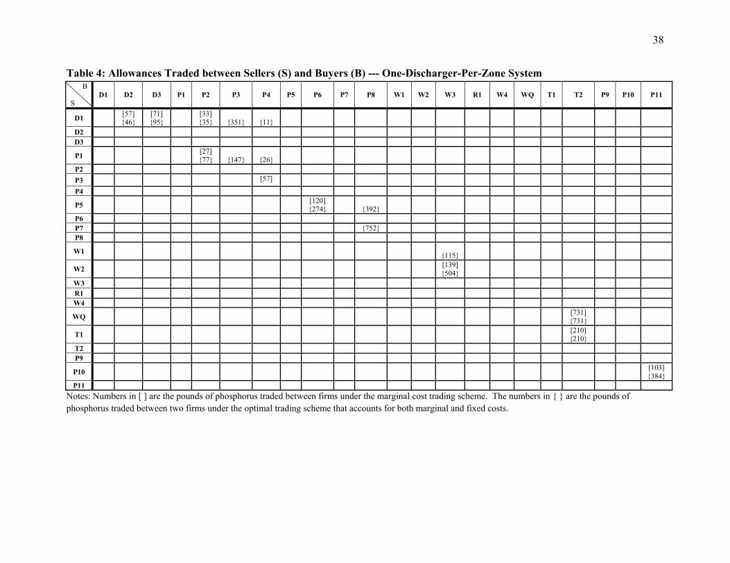
the bracketed numbers, ‘[ ]’, in Table 4. There are eight WWTPs (D1, P1, P3, P5, W2, WQ, T1

and P10) that act as sellers, and eight WWTPs (D2, D3, P2, P4, P6, W3, T2 and P11) buy

permits. Overall trade volume is very low, due to the limited trading opportunities as a result of

prohibiting upstream or cross-tributary trading and the reliance on marginal, O&M cost-based

trading. In total, only 1,549 units are traded, just over 2% of the total allowable emissions in the

watershed. As expected with downstream trading, all trades between the buyers and sellers are

indicated above the main diagonal in the trading pattern matrices. Most of these trades are

between immediately adjacent WWTPs.

Under Marginal Cost Trading, only O&M costs are considered in the cost minimization

problem and no changes in capital investments relative to the baseline are available. As such,

while the concentration level after trading does change from the no-trade levels (see Table 6,

column 3), the capital investment in abatement technology remains at the no-trade level reported

22

in Table 1, column 13. Under this trading system, total costs fall a nominal $23,489, or 0.57%

relative to the no-trade case, with savings being attributed solely to reduced O&M costs. This

small level of savings is attributed to the limitations placed on trading opportunities. Moreover,

there are no capital cost savings because each firm is assumed to invest in the capacity to

independently meet the no-trade TMDL standard.

Marginal Cost Trading, Management Area Approach: Under this trading structure, inter-MA

trading is allowed from the Upper Passaic MA to the Lower Passaic MA, and from the Pompton

MA to the Lower Passaic MA. Moreover, trades are allowed from the Pompton MA to the Upper

Passaic MA, but not the reverse. The trading ratios under this configuration are specified in

Table 3. Recall that these trading ratios are no longer bounded by one, indicating that sources can

sell allowances to firms hydrologically more distant from the relevant critical location.

The trading pattern that results from this trading rule is depicted by the numbers in ‘[ ]’s

in Table 5. Seven WWTPs (W4, WQ, T1, R1, P8, P9 and P10) act as sellers, and 14 WWTPs

(D1-D3, P1-P4, P6, P7, W1-W3, T2 and P11) buy allowances. Interestingly, most of these trades

occur with sellers located hydrologically downstream from buyers, as indicated by the

predominance of trading entries below the main diagonal of the trading matrices. This is largely

due to the geographical/hydrological organization of firm sizes, namely, large efficient firms

with lower marginal abatement costs happen to be located downstream. Another factor is that

most trading ratios for upstream trading are greater than or equal to one, as the discharges from

upstream firms have less impact at the end-point. The volume of trade increases notably

compared with the One-Discharger-Per-Zone TRS approach. There are 3,663 units of allowances

traded, representing nearly 5% of the total allowable emissions in the watershed.

23

Despite the additional trading activity, the cost savings remain nominal. The total cost

savings are $41,385 or 1.02% relative to the baseline. Hence, the added flexibility associated

with the MA approach does not engender cost-savings under marginal cost trading in which each

firm is assumed to invest in the capacity to independently meet the NPDES TMDL standard.

Optimal Trading, One-Discharger-One-Zone: In this scenario, incentives for allowance trading

are embodied not only in the differential marginal O&M costs, but also in avoiding costly capital

upgrades. It is expected that some WWTPs would buy enough allowances to avoid facility

upgrades and maintain a lower level of capital cost. Trading ratios are again defined in Table 2.

The resulting pattern of trades is reported in ‘{ }’s in Table 4. Nine WWTPs (D1, P1, P5, P7,

W1, W2, WQ, T1 and P10) act as sellers, and 10 WWTPs (D2, D3, P2 - P4, P6, P8, W3, T2 and

P11) buy permits.

Compared with marginal cost trading under the same trading ratio conditions, the optimal

trading system has much larger trading volumes as the incentive to avoid capital upgrade

stimulates more trades. There are 4,150 units of allowances traded, about 2.6 times as many as in

the marginal cost trading. This represents about 5% of the total allowable watershed emissions.

The optimal trading scenario assumes optimal capital upgrades, that is, the aggregate

watershed costs of abatements consisting of both aggregate O&M costs and aggregate Capital

upgrade costs are jointly minimized through allowance trading. Under these conditions, the

watershed annualized capital costs fall a considerable $237,787, amounting to a 14.8% reduction

relative to the baseline capital costs. Interestingly, the watershed OM costs after the trades is

slightly higher than the no-trade baseline as many allowances are sold from high marginal cost

WWTPs to low marginal cost WWTPs, driven by the incentive to avoid capital upgrade cost.

The resulted total cost-savings is $221,927 (or over 5.5% relative to the no trade baseline), with

24

all savings being attributed to the reduced capital costs. This level of total savings is about 10

times of those attained under the marginal cost trading under the same conditions.

Optimal Trading, Management Area Approach: The trading ratios under this configuration of

the MAs are specified in ‘{ }’ Table 5 according to the relative effects of each transaction on the

buyer's endpoints. All 22 WWTPS participate in trading: six (R1, W4, WQ, T1, T2 and P9) act

as sellers, and 16 (D1 - D3, P1 - P8, W1 - W3, P10 and P11) buy permits. Among the five

sellers, WQ and T1 are currently abating to less than 0.4mg/L, over-complying with the

prospective NDPES requirements. Therefore, they can simply dump their excess allowances into

the market.vii The other three sellers, W4, R1, P9, do not have present capacity to meet the

NDPES. It is expected that they will upgrade their abatement capacities fully and then sell the

leftover allowances to the buyers. On the other hand, the sixteen buyers can avoid upgrading

their facilities fully (e.g. to level 3) by acquiring allowances from the sellers. This pattern of

trade, which conforms to a priori expectations, can be summarized as follows: Large firms

(taking advantage of economies of scale in capital treatment costs), that are well positioned (in

terms of trading ratios relative to ambient measurement points) become sellers, allowing the

higher than average cost, capital intensive smaller WWTPs to avoid full upgrades. Specifically,

among the three WWTPs that upgrade fully and become sellers: W4 is the largest (and most

efficient) WWTP in the watershed; R1 is the second largest WWTP in the watershed, and, due to

external factors it has already adopted a biological treatment technology which has relatively

lower cost elasticity of abatement than the chemical technology (i.e. more efficient when treating

to a low concentration level); and P9 has the highest flow in the Lower Passaic MA.

Compared with the marginal cost trading, the optimal trading results in much larger

trading volumes as the incentive to avoid capital upgrade stimulates more trades. There are 9,618

25

units of allowances traded, nearly three times as many as in the marginal cost trading. The

volume of trade represents nearly 13% of the total allowable emissions in the watershed

Under optimal trading, MA system, trading generates substantial capital cost savings, to

the order of $538,415 (or 33.4% relative to the baseline capital costs). However, this benefit of

avoiding capital upgrade costs for some firms is offset somewhat through an increase in variable

abatement costs. As a result, the watershed OM costs after the optimal trading are slightly higher

than those in the no-trade baseline for both Multiple Source MA approaches. In total, the cost

savings for Optimal Trading MA $523,417 (13.1% relative to the baseline total costs), nearly

eight times that of the Marginal Cost Trading.

On Prices and Willingness to Pay for Permits

For any interior equilibrium of the Marginal Cost Trading, the competitive price of pollution

allowances at each WWTP is equal to its marginal abatement cost. Pollution allowances are

traded to the point where the spatially adjusted equi-marginal condition holds. There is a unique

price at each location: that is, the price of allowances at the seller’s location must be equal to the

price at the buyer’s location adjusted by the trading ratio.

For example, as indicated in Table 3, under the Marginal Cost – MA System the trading

ratio between R1 and D1 is 0.809, and R1 sells 339 allowances to D1 (see Table 5). Table 6,

Column 8 indicates that the allowances price at R1 is equal to 21.2 $/lbs, and the price at D1 is

26.2 $/lbs. These numbers verify the spatially adjusted equi-marginal condition at the internal

equilibrium, as $26.2 multiplied by 0.809 is equal to $21.2. Note that the allowances prices at

WQ and T1 cannot be determined because their non-degradation constraints are binding at the

equilibrium. Comparing the prices in the fifth and eighth columns of Table 6, allowance prices

26

are more equalized under the MA System. This is because the MA System provides more trading

opportunities than the One-Discharger-Per-Zone TRS.

The optimal trading scenarios differ from marginal cost trading in that the prices for

allowances may not be uniquely determined for some trades. This is because many WWTPs

operate at their maximum abatement capacity in equilibrium so as avoid upgrading to the higher

level. Under these “corner” conditions, although ranges for willingness to pay (WTP) and

willingness to sell (WTS) can be determined for potential trading partners, the price associated

with a transaction is not unique, varying with the bargaining power of the traders.

To this point, we have not specified numerical values for maximum WTP for additional

permits when firms are operating at the uppermost limit of their present capital investment. We

have only indicated that it will be bounded from above by the penalty for emitting without an

allowance. In the following discussion we assume that the penalty for non-compliance is set at a

sufficiently high level that all potential buyers will prefer to buy allowances in the market.

Given this assumption, if a firm has the option to upgrade then its maximum WTP is the

difference in total costs between the baseline no trading scenario and the optimal trading

outcome of the firm, divided by the change in allowances needed between the two settings (i..e.

It is the permit price at which the buyer is indifferent between participating in optimal trading

and the baseline no trade case.). This of course assumes that the buyer is guaranteed the supply

of permits to avoid the upgrade.

In this manner, WTP can be viewed as an incremental cost (US EPA, 2004; Caplan,

2008), computed as the average cost saving per unit of abatement by not having to meet the

standard without trading. For instance, the WTP of D1 is $62.60 per unit allowance which is

equal to D1’s total cost savings from the trade, $52,708, divided by the number of allowances

27

bought, 842. Drawing from the previous tables, Table 7 presents the amount and source of

allowances purchased in the optimal setting, and the derived maximum WTP of all buyers in the

Optimal Trade MA System.

In a similar fashion, sellers’ WTS can be defined as the lowest average price per

allowance the seller is willing to sell its allowances based on comparisons between the optimal

and no trade scenarios. Since for sellers operating at an interior optimum, the minimum WTS is

equal to the average marginal cost of treatment based over the range between the no-trade and

optimal trade scenarios. These values are as follows: R1 = $23.80, W4 = $25.64, P9 = $25.89

and T2=$24.00. The minimum WTS for WQ and T1 is zero, due to the fact that the current

unregulated abatements by WQ and T1 already over-comply with the required target. Thus, they

can simply dump all their unused allowances without any additional cost.

A comparison between paired WTS and WTP values indicates a wide range for

bargaining. For example, if we assume that all firms pay the lowest WTP in the group of buyers

associated with the seller R1 (i.e. there is not price discrimination amongst the buyers), then the

range of possible prices is $23.80 to $52.79, and even wider if price discrimination across buyers

does occur. The determination of this possible range is based on a set of simplifying

assumptions, whereas the actual market mechanism may be more complex. For example, it is

assumed that if a firm cannot reach the deal with its designated trading partners, it will be

excluded from the market, and so it has to independently abate to the required environmental

standard. Yet, in practice, the firm may be able to form an alternative coalition where it can

generate a higher cost savings. In this sense, the above example provides only a very rough

estimate of the range of possible price to demonstrate the complications associated with capital

cost edges in price negotiation. A refined price range could be derived using the concept of

28

"Core" in the cooperative game theory. This refined price range should be contained in the price

range provided above and is not explored further in this study.

Summary and Discussion

The principal findings from this research can be organized into three main results.

Result 1: The maximum total costs savings from the various MA approaches are nominal under

the marginal cost trading, ranging from 0.57% to 1.02% relative to the no trade scenario. This

low level of savings follows a priori expectations. Recall that there are only two treatment

technologies currently existing in the Passaic Watershed, so the differences in marginal

abatement costs arise primarily from differences in the economies of scale based on flow levels.

Hence, it should not be surprising that the volumes of trade account for only 2% to 6% of the

total allowable emissions in the watershed. These small trading volumes and disappointing

saving results are consistent with the experience from extant water quality trading programs.

Result 2: In sharp contrast with the marginal cost trading, the Optimal Trading, MA approach

yields relatively optimistic saving results, generating about 10 times of the savings as the

marginal cost trading under the same MA approach. With optimal allocation of the capacity

upgrade, the maximum percentage cost savings from the various trading regimes range from

to 13.1% relative to the no-trade scenario. The trading volume rises considerably. Specifically,

the volume of trade accounts for between 5% to 14% of the total allowable emissions in the

watershed. As the result, almost all buyers end up being able to acquire enough allowances to

stay within the maximum capacity of capital level 2 (i.e. emissions related to higher than

0.5mg/L concentration). They can take advantage of economies of scale associated with a few

large, hydrologically well-situated firms and do not need to upgrade their abatement capital to

the level 3 as in the no-trade baseline scenario. It is also important to note that, as the trading

29

equilibrium deviates from the equi-marginal point, the variable OM costs are not necessarily

minimized. However, the savings on the discrete capital costs outweigh the increase in O&M

costs, and thus greater total savings are realized.

Result 3: The percentage savings increase as different alternatives of the MA Approach become

less restrictive. The One-Discharger-Per-Zone TRS Approach does not allow increased

phosphorous load at any point in the watershed relative to the original NDPES. Permitting

upstream trade within MAs generates twice as much savings as in the One-Discharger-Per-Zone

TRS Approach. These additional cost savings are due in large measure to an ability to trade in

any direction within an MA. As a result, some low-cost downstream plants can now sell permits

to high abatement cost plants located upstream. When capital planning is feasible, these

expanded trading opportunities allow some high-cost upstream plants to avoid additional capital

investments while still avoiding increased concentrations in potential hot spots.

The above results suggest that moderate cost savings from trading phosphorus allowances

can be achieved through the MA approach (Result 3) and that substantial gains are possible if

trades can facilitate the efficient allocation of fixed cost investments across WWTPs (Result 2).

The former issue is primarily driven by the hydrology of a particular watershed and whether

managing water quality in a flexible way to protect a selected number of locations is deemed

appropriate. The later issue points to the need to consider a broader concept of trading pollution

abatement responsibilities beyond simple, single-period spot markets or auctions envisioned in

canonical treatments of water quality trading.

Our work shows that with the optimal allocation of fixed-cost upgrades, the market can

be cleared at the minimum overall abatement cost for the whole watershed through trading of

emissions allowances. This is because large, well located WWTPs can engender substantial

30

watershed-wide costs savings by upgrading and accepting treatment responsibilities for several

smaller WWTPs simultaneously. In practice, however, it would be very difficult for firms to

achieve the optimal fixed-cost upgrade allocation under spot market conditions. Due to the

discrete nature of the capital upgrades, firms cannot instantaneously adjust their abatement

capacities according to the actual trading outcomes in the market. Instead, firms need to make ex

ante capacity choices before entering the spot market. In some cases where too few WWTPs

choose to upgrade, the market cannot be cleared at any price. Moreover, since the capital

investment is irreversible, even if the market is cleared at some price, it is unlikely to be optimal

(For example, the Marginal Cost Trading scenarios give the savings estimates in the case of a

precautionary over-investment). Hence, to accomplish this objective in practice, risk averse

buyers will likely need assurances that adequate allowances will be available if they choose not

to upgrade to a capacity that would allow them to independently meet TMDL standards. Sellers

too would benefit from knowing that they will have a market for any excess allowances.

To an extent, contemporary policy experiments offer possible approaches to addressing

the capital investment problem. For example, the clearing house approach used in the

Pennsylvania water quality trading program allows forward-contract auctions, and has thus far

demonstrated the capacity to meet these contracts (O’Hara et al., 2012). Moreover, anecdotal

evidence suggest that these trades have largely involved buyers seeking to avoid costly capital

investments (Shortle, Personal Communication) Likewise, the success of the Long Island

Sound Nitrogen Credit Exchange program can be linked to the smoothing of investments by

establishing a fixed annual price for nitrogen credits and having the State of Connecticut absorb

or cover any market imbalances. As such the program acts more like an exceedance

31

tax/abatement subsidy approach in which the annual establishment of a reasonable credit price

guarantees the availability of available credits to buyers and a market for sellers.

While these programs may be effective, it is incumbent upon economists and policy

makers to more broadly conceptualize what least cost trading would involve. We note in

closing that while the cost savings demonstrated herein are not large in absolute terms, the

relative savings of 13% identified in the Optimal Trading, Management Area approach are likely

worth pursuing when aggregated across states and the entire nation. As an example, New York

State alone anticipates $36 billion in waste water treatment infrastructure over the next 20 years.

(NYS DEC).

32

References: Bandyhyopadhyay, S. and J. Horowitz, 2006. “Do Plants Overcomply with Water Pollution

Regulations? The Role of Discharge Variability.” Topics in Econ. Anal. and Policy, 6(1):1-30.

Bennett, L.L., S. G. Thorpe, and A.J. Guse, 2000, "Cost-Effective Control of Nitrogen Loadings in Long Island Sound," Water Res. Res. 36(12): 3711–3720.

Caplan, A.J., 2008. “Incremental and Average Control Costs in a Model of Water Quality Trading with Discrete Abatement Units.” Environ. and Res. Econ. 41:419-435.

David, M., W. Eheart, E. Joeres, and E. David, 1980. “Marketable Permits for the Control of Phosphorus Effluent in to Lake Michigan.” Water Res. Res. 16:263-270.

Devlin, R.A. and R.Q. Grafton, 1998. Economic Rights and Environmental Wrongs: Property Rights for the Common Good. Cheltenham: Edward Elgar.

Earnhart, D., 2004a. “Regulatory Factors Shaping Environmental Performance at Publicly-Owned Treatment Plants.” J. of Environ. Econ. and Manag. 48:6555-681.

Earnhart, D. 2004b. “The Effects of Community Characteristics on Polluter Compliance Levels.” Land Econ., 80(3): 408-432.

Eheart, J.W., 1980. “Cost Efficiency of Transferable Discharge Permits for the Control of BOD Discharges, Water Res. Res., 16:980-986.

Eheart, J.W., E.F. Joeres, and M.H. David, 1980. “Distribution Methods for Transferable Discharge Permits.” Water Res. Res., 16:833-843.

Faeth, P., 2006. “Point-Nonpointillism: The Challenges that Water Quality Trading Faces and What We Might Do About It.” Paper presented at the Second Nation Water Quality Trading Conference, May 23-25 Pittsburgh, PA. (http://www.envtn.org/WQT_EPA/Microsoft%20Word%20-%20Faeth%20Point%20NonPointillism%20Final.pdf )

Fisher-Vanden, K. and S. Olmstead, 2013. “Moving Pollution Trading from Air to Water: Potential, Problems, and Prognosis.” J. of Econ. Persp., 27(1):147-172.

Hamstead, Z.A., and T.K. BenDor, 2010. “Nutrient Trading for Enhanced Water Quality: A Case Study of North Carolina’s Neuse River Compliance Association.” Environ. and Planning: C 28(1):1‐17.

Hanley, N., R. Faichney, A. Munro, and J.S. Shortle, 1998. “Economic and Environmental Modeling for Pollution Control in an Estuary.” J. of Environ and Manag. 52:211-225.

Hoag, D.L. and J.S. Hughes-Popp, 1997. “Theory and Practice of Pollution Credit Trading in Water Quality Management.” Rev. of Agr. Econ. 19(2):252-262 .

Hung, M-F., and D. Shaw, 2005. “A Trading-Ratio System for Trading Water Pollution Discharge Permits.” J. of Env. Econ. and Manag. 49:83-102.

Jiang, F., M.B. Beck, R. G. Cummings, K. Rowles, and D. Russell (2005), Estimation of costs of phosphorus removal in wastewater treatment facilities: Adaptation of existing facilities, Water Policy Working Pap. 2005– 011, Georgia State Univ., Atlanta.

King, D.M., 2005. “Crunch Time for Water Quality Trading.” Choices, 1st Quarter. (http://www.choicesmagazine.org/scripts/printVersion.php?ID=2005-1-14 )

King, D.M., and P.J. Kuch, 2003. “Will Nutrient Credit Trading Ever Work? An Assessment of Supply and Demand Problems and Institutional Obstacles.” Environ. Law Rep. 33:10352-10368.

Kneese, A.V., and B.T. Bower, 1968. Managing Water Quality: Economics, Technology, Institutions. Washington D.C.: Resources for the Future Press.

33

Konishi, Y., J.S. Coggins, and B. Wang, 2013. “Water Quality Trading: Can We Get the Price of Pollution Right? Paper presented at AERE Summer Meetings, Banff CA., June 2013.

Morgan, C., and A. Wolverton, 2005."Water Quality Trading in the United States." National Center for Environmental Economics Working Paper 05-07.

Najarian Associates. 2005. "Development of a TMDL for the Wanaque Reservoir and Cumulative WLAs/LAs for the Passaic River Watershed." Project Report submitted to the New Jersey Department of Environmental Protection.

Nutrient Reduction Technology Cost Task Force (NRTCTF), 2002. Nutrient reduction technology cost estimations for point sources in the Chesapeake Bay Watershed. A Report to the Chesapeake Bay Program, MD: Annapolis.

New Jersey Department of Environmental Protection (NJDEP), 2008. Total Maximum Daily Load Report for the Non-Tidal Passaic River Basin Addressing Phosphorus Impairments, Watershed Management Areas 3, 4 and 6.

New York State Department of Environmental Conservation (NYS DEC). “A Gathering Storm: New York Wastewater Infrastructure in Crisis.” http://www.dec.ny.gov/chemical/48803.html

Obrupta, C.C., M. Niazi, J.S. Kardos, 2008. “Application of an Environmental Decision Support System to a Water Quality Trading Program Affected by Surface Water Diversions.” Environ. Manag. 42:946–956.

O’Hara, j.K., M.J. Walsh, P.K. Marchetti, 2012. “Establishing a Clearing House to Reduce Impediments to Water Quality Trading.” The J. of Region. Anal. and Pol. 42(2): 139-150.

Omni Environmental Corporation, 2007. The Non-Tidal Passaic River Basin Nutirent TMDL Study Phase II Watershed Model and TMDL Calculations: Final Report. Princeton, Omni Environmental Corporation.

Rose-Ackerman, S., 1973. “Effluent Charges: A Critique.” Can. J. of Econ. 6:512-528. Sado, Y., R.N. Boisvert and G.L. Poe, 2010. “Potential Cost Savings from Discharge Permit

Trading: A Case Study and Implications for Water Quality Trading.” Wat Res. Res. 44:020501

Schmalensee, R., and R.N. Stavins, 2013. "The SO2 Allowance Trading System: The Ironic History of a Grand Policy Experiment." J. of Econ. Persp., 27(1): 103-22.

Shortle, J., Personal Communication. Selman, M., S. Greenhalgh, E. Branosky, C. Jones, and J. Guiling, 2009. “Water Quality Trading

Programs: An International Overview” WRI (World Resources Institute) Issue Brief: Water Quality Trading No. 1.

Suter, J.F., J. Spraggon, and G.L. Poe, 2013. “Thin and Lumpy: An Experimental Investigation of Water Quality Trading”. Water Res. and Econ. 1:36-60.

Stephenson, K. and L. Shabman, 2011. “Rhetoric and Reality of Water Quality Trading and the Potential for Market-like Reform.” J. of the Amer. Water Res. Assoc. 47: 15–28.

Tietenberg, T.H., 2006. Emissions Trading: Principles and Practice. Washington D.C.: Resource for the Future.

US EPA, 1996. Draft Framework for Watershed-Based Trading, Office of Water, Washington DC. (http://www.epa.gov/owow/watershed/framewrk/framwork.htm)

US EPA, 2004. Water Quality Trading Assessment Handbook: Can Water Quality Trading Advance Your Watershed’s Goals? (http://www.epa.gov/owow/watershed/trading/handbook/ )

34

US EPA, 2008. EPA Water Quality Trading Evaluation Final Report (http://www.epa.gov/evaluate/wqt.pdf )

Woodward, R.T., 2003. “Lessons about Effluent Trading from a Single Trade.” Rev. of Agr. Econ. 25(1):235-245.

Woodward, R.T. and R. A. Kaiser, 2002a. “Market Structures for U.S. Water Quality Trading.” Review of Agricultural Economics 24(2):366-383.

Woodward, R.T., R.A. Kaiser, and A-M B. Wicks, 2002b. “The Structure and Practice of Water Quality Trading Markets.” J. of the Amer. Water Res. Assoc. 38(4):967-979.

Zhao, T., 2013. “Economic Modeling of Point-to-Point Source Water Quality Trading in the Upper Passaic Watershed Accounting for Fixed and Variable Costs.” Unpublished MS Thesis, Dyson School of Applied Economics and Management, Cornell University.

Table 1: Descriptive Statistics for Passaic Waste Water Treatment Plants (WTPS) for Phosphorus (P) Descriptive Statistics Annualized Capital Costs by Investment Level ($) No Trade Scenario

(1) (2) (3) (4) (5) (6) (7) (8) (9) (10) (11) (12) (13) (14) (15)

Management Area

River WWTP Map Code

Avg. Flow

(MGD)

Initial Phosp. Conc. (mg/l)

Treatment Tech.

Xi = 0 Xi = 1 Xi = 2 Xi = 3 Xi = 4 Xi = 5 Concentration (mg/l) /

Capital Level (Xi)

Total Annual

Cost ($)

Marginal Cost ($) P ≥

1.50 mg/l

P ≥ 1.00 mg/l

P ≥ 0.50 mg/l

P ≥ 0.25 mg/l

P ≥ 0.10 mg/l

P ≥ 0.05 mg/l

Upper Passaic

Dead D1 1.76 3.13 Chemical 11,121 17,074 35,533 73,949 194,849 405,503 0.4 / 3 147,733 33.17 Dead D2 0.15 1.85 Chemical 5,377 7,265 12,152 20,327 40,125 67,116 0.4 / 3 31,856 67.96 Dead D3 0.31 1.91 Chemical 6,662 9,346 16,674 29,745 63,934 114,057 0.4 / 3 49,672 55.07

Passaic P1 1.00 2.63 Chemical 9,412 14,033 27,775 54,976 135,564 268,323 0.4 / 3 103,158 39.15 Passaic P2 0.36 1.67 Chemical 6,962 9,844 17,796 32,172 70,374 127,221 0.4 / 3 54,477 52.73 Passaic P3 1.57 0.60 Chemical n/a n/a/ 33,808 69,649 181,075 373,039 0.4 / 3 103,537 34.30 Passaic P4 0.12 1.53 Chemical 5,035 6,724 11,026 18,082 34,771 57,022 0.4 / 3 27,826 72.48 Passaic P5 2.41 3.28 Chemical 12,202 19,042 40,749 87,201 238,394 510,158 0.4 / 3 180,712 30.24 Passaic P6 0.90 1.48 Chemical 9,124 13,529 26,529 52,021 126,701 248,448 0.4 / 3 96,524 40.37 Passaic P7 2.61 2.63 Chemical 12,492 19,576 42,189 90,924 250,908 540,748 0.4 / 3 190,228 29.54 Passaic P8 3.75 1.62 Chemical 13,902 22,199 49,406 109,657 316,605 704,631 0.4 / 3 240,458 26.54

Whippany W1 1.90 0.84 Biological n/a n/a 83,836 122,913 203,823 298,826 0.4 / 3 151,234 31.21 Whippany W2 3.03 0.56 Biological n/a n/a 113,615 167,333 279,163 411,153 0.4 / 3 212,841 26.99 Whippany W3 2.03 2.83 Chemical 11,599 17,941 37,813 79,696 213,537 450,060 0.4 / 3 161,862 31.80 Rockaway R1 12.58 2.98 Chemical n/a 151,933 226,089 336,442 569,002 846,726 0.4 / 3 532,433 19.13 Whippany W4 8.81 1.46 Biological 19,871 33,786 83,717 207,442 688,404 1,705,786 0.4 / 3 541,009 18.52

Pompton Wanaque WQ 1.00 0.16 Biological n/a n/a n/a n/a 135,564 268,323 0.16 / 4 133,993 38.31 Pompton T1 0.86 0.32 Chemical n/a n/a n/a 50,795 123,058 240,333 0.32 / 3 53,736 40.91 Pompton T2 5.33 2.14 Chemical 15,422 25,079 57,585 133,222 396,741 910,960 0.4 / 3 302,329 23.92

Lower Passaic

Signac Brook P9 7.47 2.27 Chemical 17,038 28,196 66,709 157,827 492,698 1,165,679 0.4 / 3 377,225 21.63

Peckman P10 2.46 3.07 Chemical 12,276 19,178 41,115 88,145 241,557 517,867 0.4 / 3 183,115 30.06

Peckman P11 1.26 2.25 Chemical 10,077 15,205 30,718 62,060 157,237 317,669 0.4 / 3 119,411 36.59

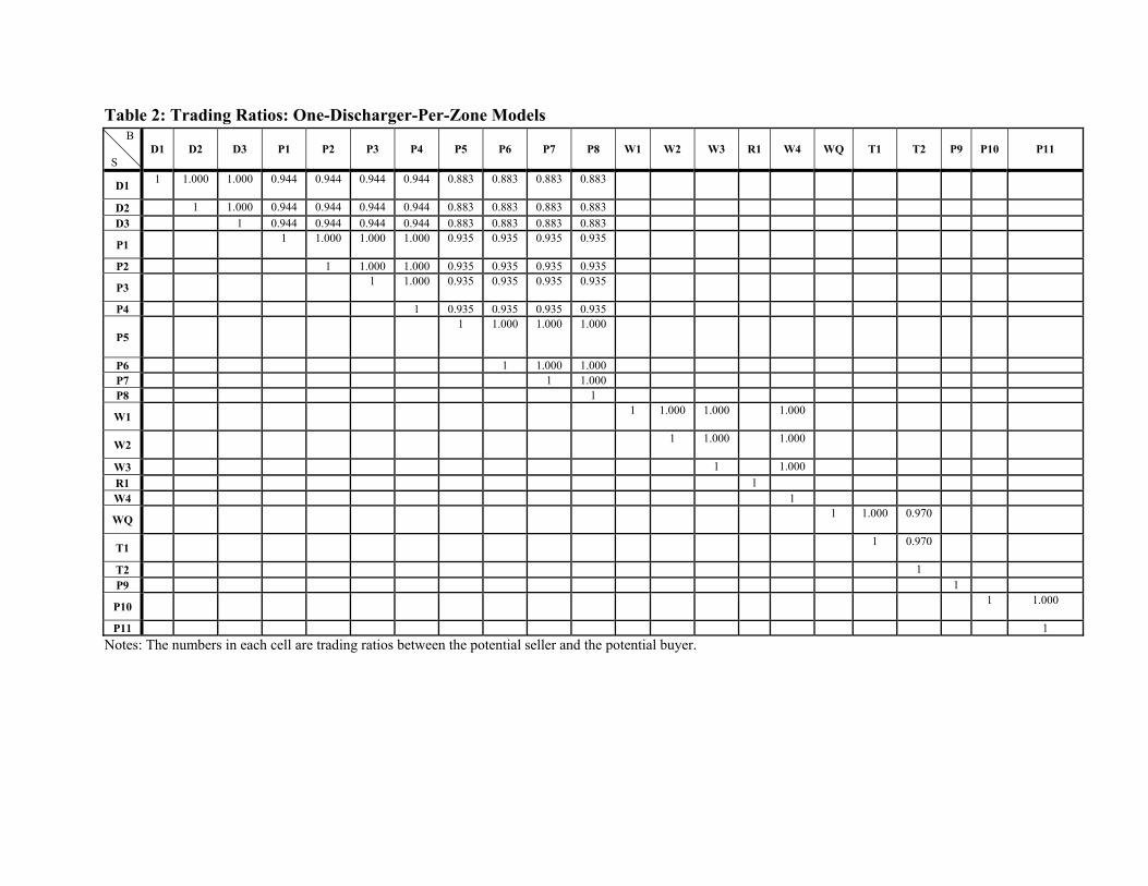
Table 2: Trading Ratios: One-Discharger-Per-Zone Models B

S D1 D2 D3 P1 P2 P3 P4 P5 P6 P7 P8 W1 W2 W3 R1 W4 WQ T1 T2 P9 P10 P11

D1 1 1.000 1.000 0.944 0.944 0.944 0.944 0.883 0.883 0.883 0.883

D2 1 1.000 0.944 0.944 0.944 0.944 0.883 0.883 0.883 0.883 D3 1 0.944 0.944 0.944 0.944 0.883 0.883 0.883 0.883

P1 1 1.000 1.000 1.000 0.935 0.935 0.935 0.935

P2 1 1.000 1.000 0.935 0.935 0.935 0.935

P3 1 1.000 0.935 0.935 0.935 0.935

P4 1 0.935 0.935 0.935 0.935

P5 1 1.000 1.000 1.000

P6 1 1.000 1.000 P7 1 1.000 P8 1

W1 1 1.000 1.000 1.000

W2 1 1.000 1.000

W3 1 1.000 R1 1 W4 1

WQ 1 1.000 0.970

T1 1 0.970

T2 1 P9 1

P10 1 1.000

P11 1 Notes: The numbers in each cell are trading ratios between the potential seller and the potential buyer.

37

Table 3: Trading Ratios – Management Area Models B

S D1 D2 D3 P1 P2 P3 P4 P5 P6 P7 P8 W1 W2 W3 R1 W4 WQ T1 T2 P9 P10 P11 D1 1 1.000 1.000 0.944 0.944 0.944 0.944 0.883 0.883 0.883 0.883 1.026 1.026 1.026 1.147 1.026 0.599 0.440 0.440 D2 1.000 1 1.000 0.944 0.944 0.944 0.944 0.883 0.883 0.883 0.883 1.026 1.026 1.026 1.147 1.026 0.599 0.440 0.440 D3 1.000 1.000 1 0.944 0.944 0.944 0.944 0.883 0.883 0.883 0.883 1.026 1.026 1.026 1.147 1.026 0.599 0.440 0.440 P1 1.024 1.024 1.024 1 1.000 1.000 1.000 0.935 0.935 0.935 0.935 1.053 1.053 1.053 1.176 1.053 0.634 0.466 0.466 P2 1.024 1.024 1.024 1.000 1 1.000 1.000 0.935 0.935 0.935 0.935 1.053 1.053 1.053 1.176 1.053 0.634 0.466 0.466 P3 1.024 1.024 1.024 1.000 1.000 1 1.000 0.935 0.935 0.935 0.935 1.053 1.053 1.053 1.176 1.053 0.634 0.466 0.466 P4 1.024 1.024 1.024 1.000 1.000 1.000 1 0.935 0.935 0.935 0.935 1.053 1.053 1.053 1.176 1.053 0.634 0.466 0.466 P5 1.024 1.024 1.024 1.000 1.000 1.000 1.000 1 1.000 1.000 1.000 1.105 1.105 1.105 1.235 1.105 0.678 0.499 0.499 P6 1.024 1.024 1.024 1.000 1.000 1.000 1.000 1.000 1 1.000 1.000 1.105 1.105 1.105 1.235 1.105 0.678 0.499 0.499 P7 1.024 1.024 1.024 1.000 1.000 1.000 1.000 1.000 1.000 1 1.000 1.105 1.105 1.105 1.235 1.105 0.678 0.499 0.499 P8 1.024 1.024 1.024 1.000 1.000 1.000 1.000 1.000 1.000 1.000 1 1.105 1.105 1.105 1.235 1.105 0.678 0.499 0.499

W1 0.927 0.927 0.927 0.905 0.905 0.905 0.905 0.857 0.857 0.857 0.857 1 1.000 1.000 1.115 1.000 0.582 0.427 0.427

W2 0.927 0.927 0.927 0.905 0.905 0.905 0.905 0.857 0.857 0.857 0.857 1.000 1 1.000 1.115 1.000 0.582 0.427 0.427 W3 0.927 0.927 0.927 0.905 0.905 0.905 0.905 0.857 0.857 0.857 0.857 1.000 1.000 1 1.115 1.000 0.582 0.427 0.427 R1 0.809 0.809 0.809 0.764 0.764 0.764 0.714 0.714 0.714 0.714 0.714 0.833 0.833 0.833 1 0.833 0.485 0.356 0.356

W4 0.927 0.927 0.927 0.905 0.905 0.905 0.905 0.905 0.857 0.857 0.857 1.000 1.000 1.000 1.118 1 0.582 0.427 0.427

WQ 0.637 0.637 0.637 0.602 0.602 0.602 0.602 0.563 0.563 0.563 0.563 0.656 0.656 0.656 0.788 0.656 1 1.000 1.000 0.382 0.280 0.280

T1 0.637 0.637 0.637 0.602 0.602 0.602 0.602 0.563 0.563 0.563 0.563 0.656 0.656 0.656 0.788 0.656 1.000 1 1.000 0.382 0.280 0.280

T2 0.657 0.657 0.657 0.620 0.620 0.620 0.620 0.580 0.580 0.58 0.580 0.677 0.677 0.677 0.812 0.677 1.000 1.000 1 0.393 0.289 0.289

P9 1 0.735 0.735

P10 0.978 1 1.000

P11 0.978 1.000 1

Notes: The numbers in each cell are trading ratios between the potential seller and the potential buyer. Bolded numbers indicate cell entries that differ from those in Table 2.

38

Table 4: Allowances Traded between Sellers (S) and Buyers (B) --- One-Discharger-Per-Zone System B

S D1 D2 D3 P1 P2 P3 P4 P5 P6 P7 P8 W1 W2 W3 R1 W4 WQ T1 T2 P9 P10 P11

D1 [57] {46}

[71] {95}

[33] {35} {351} {11}

D2 D3

P1 [27] {77} {147} {26}

P2 P3 [57]

P4

P5 [120] {274} {392}

P6 P7 {752} P8

W1 {115}

W2 [139] {504}

W3 R1 W4

WQ [731] {731}

T1 [210] {210}

T2 P9

P10 [103] {384}

P11 Notes: Numbers in [ ] are the pounds of phosphorus traded between firms under the marginal cost trading scheme. The numbers in { } are the pounds of phosphorus traded between two firms under the optimal trading scheme that accounts for both marginal and fixed costs.

Table 5: Allowances Traded between Sellers (S) and Buyers (B) --- Management Area System B

S D1 D2 D3 P1 P2 P3 P4 P5 P6 P7 P8 W1 W2 W3 R1 W4 WQ T1 T2 P9 P10 P11 D1 D2 D3 P1 P2 P3 P4 P5 P6 P7 P8 [97] [66]

W1

W2 W3 R1 [339] [132]

{78} [205] {117} {304} {144} {627} {67} {1268}

W4 [280] [190] [278] [98] {857}

[247] {320}

[7] {928} {277}

[384] {579}

[231] {927}

[363] {619}

WQ {732}

[731]

T1 {110} {99}

[210]

T2 {21}

P9 {1021}

[170] {523}

P10 [23]

P11 Notes: Numbers in [ ] are the pounds of phosphorus traded between firms under the marginal cost trading scheme. The numbers in { } are the pounds of phosphorus traded between two firms under the optimal trading scheme that accounts for both marginal and fixed costs.

Table 6: Descriptive Statistics for Passaic Waste Water Treatment Plants (WTPS) for Phosphorus (P)

Management Area

WWTP Map Code

Marginal Cost Trading Optimal Trading

One-Discharger-One-Zone Management Area One-Discharger-One-Zone Management Area

(1) (2) (3) (4) (5) (6) (7) (8) (9) (10) (11) (12) Concentration after Trading

(mg/L) / Capital Level.

Total Annual

Treatment Cost ($)

Price of Allowance

at Each WWTP ($)

Concentration after Trading

(mg/L) / Capital Level.

Total Annual

Treatment Cost ($)

Price of Allowance

at Each WWTP ($)

Concentration after Trading

(mg/L) / Capital Level.

Total Annual

Treatment Cost ($)

Concentration after Trading

(mg/L) / Capital Level.

Total Annual

Treatment Cost ($)

Upper Passaic

D1 0.37 153502 38.7 0.45 139662 26.2 0.30 171371 0.50 95025

D2 0.53 28933 38.7 0.63 27359 26.2 0.50 21216 0.54 20522

D3 0.48 46379 38.7 0.58 43379 26.2 0.50 32457 0.50 32457

P1 0.39 104243 40.9 0.48 94948 26.9 0.32 115475 0.50 66399

P2 0.45 51781 40.9 0.56 48004 26.9 0.50 35490 0.50 35490

P3 0.39 105555 36.4 0.45 95897 26.9 0.50 54519 0.50 54519

P4 0.56 24889 36.4 0.64 23895 26.9 0.50 18669 0.54 18063

P5 0.38 184500 32.8 0.41 177878 28.4 0.31 206580 0.50 116391

P6 0.44 92148 32.8 0.48 89354 28.4 0.50 62165 0.50 62165

P7 0.40 190228 29.5 0.41 188330 28.4 0.31 219092 0.50 122582

P8 0.40 240158 29.5 0.39 244457 28.4 0.50 155449 0.50 155449

W1 0.40 151235 31.3 0.47 140649 24.3 0.38 154984 0.50 97079

W2 0.39 216695 28.6 0.43 206926 24.3 0.35 228078 0.50 138391

W3 0.42 157666 28.6 0.46 151772 24.3 0.50 104160 0.50 104160

R1 0.40 541008 19.1 0.38 554593 21.2 0.40 541009 0.30 602900

W4 0.40 532434 18.5 0.35 576525 24.3 0.40 532433 0.28 648000

Pompton

WQ 0.16 133993 n/a 0.16 133993 n/a 0.16 133993 0.16 133993

T1 0.32 53736 n/a 0.32 53736 n/a 0.32 53736 0.32 53736

T2 0.46 284078 18.6 0.46 284078 18.6 0.46 283077 0.40 302834

Lower Passaic

P9 0.40 377225 21.6 0.39 380963 22.4 0.40 377225 0.33 417040

P10 0.39 186318 32.2 0.40 183807 30.5 0.35 196313 0.50 117953

P11 0.43 115879 32.2 0.44 114481 30.5 0.50 76802 0.50 76802

Aggregate Cost

3972581 (0.57%)

3954684 (1.02%)

3774292 (5.53%)

3471951 (13.10%)

Numbers in paranthesis are percentage cost savings relative to No Trading scenario

Table 7: Price Range for Optimal Trading Management Area System

Seller Units of

allowances sold

WTS per unit of

allowance Buyer

Units of allowances

bought

WTP per effective

allowance

WTP per unit of allowance (adj

for trading ratios) Possible price

range

R1 2604 23.80

D2 78 179.1 145.10

$23.80-$52.79

D3 117 182.1 147.53 P1** 304 120.6 91.62

P2 144 173.0 131.46 P3 627 102.4 77.82 P4 67 191.4 145.45

P8* 1268 74.3 52.79

W4 4508 25.64

P5 857 87.5 75.28

$25.64-$63.94

P6 320 125.2 107.68 P7 928 85.0 73.10

P8* 277 74.3 63.94 W1 579 93.5 93.48 W2 927 80.3 80.32 W3 619 93.2 93.22

P9 1543 25.80 P10 1021 86.9 63.42 $25.80-$63.42

P11 523 110.9 80.96 T2 21 24.00 P1** 21 120.6 74.74 $24.00-$74.74

WQ&T1 941 0.00 D1 842 98.2 62.60 $0.00-$62.60

P1** 99 120.6 72.33 * WWTPs which buy from two sellers** WWTPs which buy from three sellers

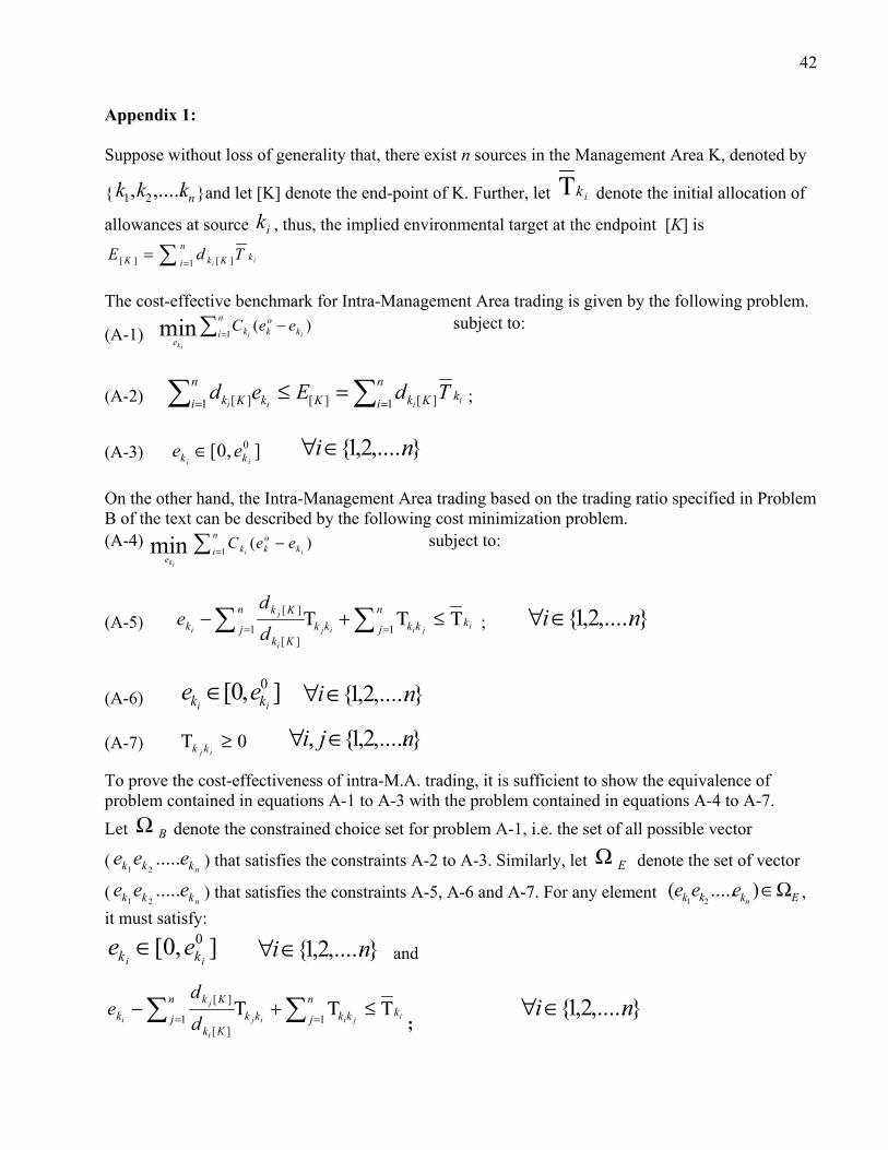
42

Appendix 1:

Suppose without loss of generality that, there exist n sources in the Management Area K, denoted by

{ nkkk ,....., 21 }and let [K] denote the end-point of K. Further, let ikΤ denote the initial allocation of

allowances at source ik , thus, the implied environmental target at the endpoint [K] is

== n

i kKkK iiTdE

1 ][][

The cost-effective benchmark for Intra-Management Area trading is given by the following problem.

(A-1) =−n

i kokk

eii

ik

eeC1

)(min subject to:

(A-2) ===≤ n

i kKkKn

i kKk iiiiTdEed

1 ][][1 ][ ;

(A-3) ],0[ 0ii kk ee ∈ },.....2,1{ ni∈∀

On the other hand, the Intra-Management Area trading based on the trading ratio specified in Problem B of the text can be described by the following cost minimization problem. (A-4) =

−n

i kokk

eii

ik

eeC1

)(min subject to:

(A-5) ijiij

i

j

ik

n

j kkkkn

jKk

Kkk d

de Τ≤Τ+Τ− == 11

][

][ ; },.....2,1{ ni∈∀

(A-6) ],0[ 0ii kk ee ∈

},.....2,1{ ni∈∀

(A-7) 0≥Τij kk },.....2,1{, nji ∈∀

To prove the cost-effectiveness of intra-M.A. trading, it is sufficient to show the equivalence of problem contained in equations A-1 to A-3 with the problem contained in equations A-4 to A-7. Let BΩ denote the constrained choice set for problem A-1, i.e. the set of all possible vector

(nkkk eee .....

21) that satisfies the constraints A-2 to A-3. Similarly, let EΩ denote the set of vector

(nkkk eee .....

21) that satisfies the constraints A-5, A-6 and A-7. For any element Ekkk n

eee Ω∈).....(21

, it must satisfy:

],0[ 0ii kk ee ∈ },.....2,1{ ni∈∀ and

ijiij

i

j

ik

n

j kkkkn

jKk

Kkk d

de Τ≤Τ+Τ− == 11

][

][

;},.....2,1{ ni∈∀

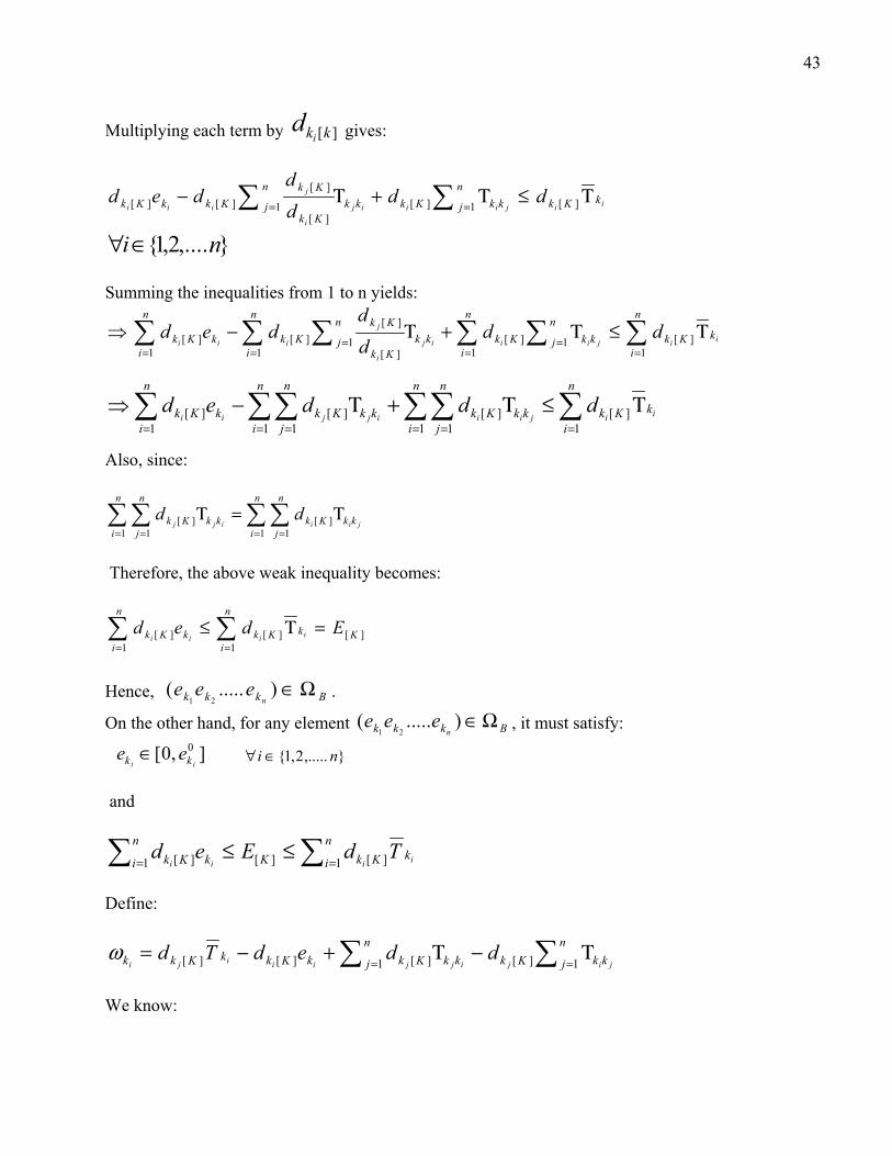
43

Multiplying each term by ][kkid gives:

iijiiij

i

j

iiikKk

n

j kkKkkkn

jKk

KkKkkKk dd

dd

ded Τ≤Τ+Τ− == ][1][1][

][][][

},.....2,1{ ni∈∀

Summing the inequalities from 1 to n yields:

=

==

===

Τ≤Τ+Τ−n

ikKk

n

j kk

n

iKkkk

n

jKk

Kkn

iKk

n

ikKk iijiiij

i

j

iiidd

dd

ded1

][11

][1][

][

1][

1][

== == ==

Τ≤Τ+Τ−n

ikKk

n

i

n

jkkKk

n

i

n

jkkKk

n

ikKk iijiiijjii

ddded1

][1 1

][1 1

][1

][

Also, since:

= == =

Τ=Τn

i

n

jkkKk

n

i

n

jkkKk jiiijj

dd1 1

][1 1

][

Therefore, the above weak inequality becomes:

][1

][1

][ K

n

ikKk

n

ikKk Eded iiii

=Τ≤ ==

Hence, Bkkk neee Ω∈).....(

21.

On the other hand, for any element Bkkk neee Ω∈).....(

21, it must satisfy:

],0[ 0ii kk ee ∈ },.....2,1{ ni ∈∀

and

==≤≤ n

i kKkKn

i kKk iiiiTdEed

1 ][][1 ][

Define:

==Τ−Τ+−= n

j kkKkkkn

j KkkKkkKkk jijijjiiijiddedTd

1][1 ][][][ω

We know:

44

=

≥n

iki

10ω

To help the demonstration, the set K is divided into three subset +K , −K and 0K , where +K is the set of firms which have positive ω , −K is the set of firms which have negative ω ; finally, 0K

is the set of firms which have 0=ω .(i) If φ=−K ,that is, if all firms have nonnegative ω , then, it is easy to verify that there exists anull matrix }0{ =Τ

ij kk s.t. (E-1), (E-2) and (E-3) are satisfied. Ekkk neee Ω∈).....(

21

(ii) φ≠−K , that is, if not all firms have nonnegativeω , let +S define the sum of all positive ikω ,

that is: =

+ =n

iki

S1

}0,max{ω . Then there exists a nonnegative matrix }{ij kkΤ with

0/ ][ >

⋅=Τ +

++−

−+ S

d Kkkk

kkjji

ij

ωω for all −− ∈ Kki , ++ ∈ Kki ; and all other elements are equal to

zero. I claim that with }0{ =Τij kk , and constraints (E-1), (E-2) and (E-3) are satisfied and so are

Ekkk neee Ω∈).....(

21

Now verify the claim: For 00 Kki ∈ constraints (E-1), (E-2) and (E-3) are trivially satisfied.

For ++ ∈ Kk j

][

][

11][

][

/)/(

KkkK

kKkk

Kkk

n

j kkkkn

jKk

Kk

jj

ijj

ijjiij

i

j

dS

d

dd

++

−−++

−−+

==

Τ=Τ+Τ−

+

==

ωωω

Therefore, constraints (A-5), (A--6) and (A-7) are satisfied. For −− ∈ Kki

45

−

++

−

+−++

==

Τ=Τ+Τ−

+

==

i

j

i

ijjjiiijj

kK

k

k

KkkKk

n

j kkKkkkn

j Kk

S

ddd

ωω

ω

][1][1 ][

Therefore, constraints (E-1), (E-2) and (E-3) are satisfied. Combining (i) and (ii), we know

Bkkk neee Ω∈).....(

21 Ekkk neee Ω∈).....(

21

Since we have already shown Ekkk n

eee Ω∈).....(21

Bkkk neee Ω∈).....(

21

Therefore, we have shown that: EB Ω=ΩSince the two minimization problems have the same objective function over the same choice set, I claim that the result of problem (B) must be the result of problem (E) and vice versa. This completes the proof that Intra-M.A. trading constraints support the cost-effective allocation of allowances subject to the environmental standard at the M.A. endpoint. QED

Appendix 2:

The corresponding Kuhn-Tucker equation for one branch of Problem C (given a set of upgrade choices) is:

K(ei, Tki, λi, αi, βi ) = =====

−−−+−Τ+Τ−+ n

i iiiin

i iiin

k ikkin

k kiin

i i xeeeTteZ11 0111

))(()()( φβαλ

By solving for the Kuhn-Tucker conditions (written in type II K-T representation), 0=−++′=∂∂ iiiii ZeK βαλ ; (i = 1,…,n)

0≤+−=Τ∂∂ kikiki tK λλ (k = 1,...,n; i = 1,…,n)

0)( =+−⋅Τ kikiki t λλ (k = 1,...n; i =1,…,n)

01

≤−Τ+Τ−=∂∂ == in

ik ikn

k kikiii TteK λ (i = 1,…,n)

===−Τ+Τ−⋅ n

k iikn

k kikiii Tte11

0)(λ (i = 1,…,n)

00 ≤−=∂∂ eeK iiα (i = 1,…,n)

46

0)( 0 =−⋅ eeiiα (k = 1,...n; i =1,…,n)

0)( ≤−=∂∂ iiii exK φβ (i = 1,…,n)

0))(( =−⋅ iiii exφβ (k = 1,...n; i =1,…,n)

Suppose that the cost functions are strongly monotonically decreasing with final effluent ( ie ). It must be the case that every firm utilizes all of its tradable permits so the trading equation is binding (i.e. ==

=Τ+Τ− n

k iikn

k kikii Tte11

). Then, each firm at an interior solution (i.e. 0== ii βα ) has a positive shadow price λi, Hung and Shaw show that these shadow prices are the prices of the permits at the respective points. Moreover, when trade takes place between k and i (e.g. Tki is strictly

positive), the following equality results: i

k

ii

ikki d

dt

λλ

===][

][ which states that the ratio of shadow

prices (as well as the ratio of prices of permits) between k and i, is just equal to the transfer coefficient between these two plants at the interior. In the interior, the complementary slackness conditions ensure that multipliers αi , βi are all equal to zero, and hence, the shadow price of a unit of effluent at site i, is equivalent to the marginal abatement cost at site i. ( i.e.

iiiiii ZMC λβαλ =−+=′−= ).There are two corner situations that would make the permit price deviate from the marginal

abatement cost: If the final effluent of plant i is bounded by the initial untreated effluent level (i.e. )00 =−eei , multipliers αi would be nonnegative. Then iiiii ZMC λαλ ≥+=′−= , showing that the

permit price at firm i could be less than its marginal cost. On the other hand, if the final effluent of plant i is bounded by its physical removal capacity (i.e. 0)( =− iii exφ ), multipliers βi would be

nonnegative. Then iiiii ZMC λβλ ≤−=′−= , showing that the permit price at i could be higher thanits marginal abatement cost.

47

Endnotes:

i The limited trading in water quality markets has been attributed to a number of institutional and program design factors, including: the lack of regulatory coverage (Faeth, 2006; Stephenson and Shabman, 2011); the lack of a binding cap on emissions (Selman et al., 2009); the limited numbers of trading opportunities (Obrupta et al., 2008); the imposed market structures (Woodward and co-authors 2002a, b; 2003); and the high transactions costs associated with complex administrative requirements (Devlin and Grafton, 1998; O’Hara et al., 2012). From a behavioral perspective, managers of individual water treatment plants may choose to over-comply and not trade in response to local demographic pressures (Earnhart 2004a, b); to account for a margin of safety or to otherwise minimize regulatory risk (Bandyopadhyay and Horowitz 2006; Selman et al., 2009); or to protect opportunities for future growth (Hamstead and BenDor, 2010). ii In their article Hung and Shaw (2005) do not explicitly address the issue of multiple dischargers within a zone. For example, they note: “ in general, the number of dischargers in a zone would be greater than or equal to one, although we assume that there is only one representative discharger in each zone.” (p. 88). Elsewhere, the authors state: “A zone can be defined as an area in which the dispersion characteristics of effluents and the environmental effects of any unit of effluent are very close.” (p. 86) iii A recent paper by Konishi et al. (2013) raises concerns about the Hung and Shaw TRS approach in cases where the trading ratios are non-associative or there exists a critical zone at the confluence of upstream branches. iv Two of the authors of the referenced article, Chris Obrupta and Josef Kardos, were collaborators with us on the US EPA-funded project “Development, Implementation, and Evaluation of a Water Quality Trading Program for the Non-Tidal Passaic River Watershed” underlying the present paper. v Zhao (2013) provides a formal proof of this proposition. vi The cost minimization problem C is formulated based on a mixed-integer nonlinear programming model. In this case study, the optimal allocation of allowances is solved on the General Algebraic Modeling System (GAMS) which provides an algorithm "DICOPT" designed for solving mixed-integer nonlinear programming problems that involve linear binary and linear and nonlinear continuous variables. The OM cost function being convex satisfies one of the necessary conditions for this algorithm to work effectively. One of the necessary conditions for DICOPT to work effectively is that the upper contour set of OM cost function must be pseudo-convex. The concavity of OM cost function guarantees the upper contour set is convex, which is a special case of pseudo-convex. vii WQ and T1 cannot abate less because they are bounded by the non-degradation principle. However, they can sell their excess allowances through market trading.

WP No Title Author(s)

OTHER A.E.M. WORKING PAPERS

Fee(if applicable)

Food Waste: The Role of Date Labels,Package Size, and Product Category

Wilson, N., Rickard, B., Saputo, R. and S.Ho

2015-07

Education for Climate Justice Kanbur, R.2015-06

Dynastic Inequality, Mobility and Equality ofOpportunity

Kanbur, R. and J.E. Stiglitz2015-05

The End of Laissez-Faire, The End of History,and The Structure of Scientific Revolutions

Kanbur, R.2015-04

Assessing the Economic Impacts of FoodHubs to Regional Economics: a frameworkincluding opportunity cost

Jablonski, B.B.R., Schmit, T.and D. Kay2015-03

Does Federal crop insurance Lead to higherfarm debt use? Evidence from the AgriculturalResource Management Survey

Ifft, J., Kuethe, T. and M. Morehart2015-02

Rice Sector Policy Options in Guinea Bissau Kyle, S.2015-01

Impact of CO2 emission policies on foodsupply chains: An application to the US applesector

Lee, J., Gómez, M., and H. Gao2014-22

Informality among multi-product firms Becker, D.2014-21

Social Protection, Vulnerability and Poverty Kanbur, R.2014-20

What is a "Meal"? Comparative Methods ofAuditing Carbon Offset Compliance for FuelEfficient Cookstoves

Harrell, S., Beltramo, T., Levine, D.,Blalock, G. and A. Simons

2014-19

Informality: Causes, Consequences and PolicyResponses

Kanbur, R.2014-18

How Useful is Inequality of Opportunity as aPolicy-Construct?

Kanbur, R. and A. Wagstaff2014-17

The Salience of Excise vs. Sales Taxes onHealthy Eating: An Experimental Study

Chen, X., Kaiser, H. and B. Rickard2014-16

Paper copies are being replaced by electronic Portable Document Files (PDFs). To request PDFs of AEM publications, write to (be sure toinclude your e-mail address): Publications, Department of Applied Economics and Management, Warren Hall, Cornell University, Ithaca, NY14853-7801. If a fee is indicated, please include a check or money order made payable to Cornell University for the amount of yourpurchase. Visit our Web site (http://dyson.cornell.edu/research/wp.php) for a more complete list of recent bulletins.