management simulation models and solvency in general insurance ___________________ nino savelli...

MANAGEMENT SIMULATION MODELS AND SOLVENCY IN GENERAL INSURANCE___________________

Nino SavelliUniversità Cattolica di Milano

VI Congresso Nazionale di Scienza e Tecnica delle AssicurazioniBologna, 18-20 Gennaio 2004

Insurance Risk Management Insurance Risk Management and Solvency :and Solvency :

MAIN PILLARS OF THE INSURANCE MANAGEMENT:MAIN PILLARS OF THE INSURANCE MANAGEMENT:market share - financial strength - return for stockholders’ capital. market share - financial strength - return for stockholders’ capital.

NEED OF NEW CAPITAL: NEED OF NEW CAPITAL: to increase the volume of business is a natural target for the to increase the volume of business is a natural target for the management of an insurance company, but that may cause a need management of an insurance company, but that may cause a need of new capital for solvency requirements and consequently a of new capital for solvency requirements and consequently a reduction in profitability is likely to occur.reduction in profitability is likely to occur.

STRATEGIES: STRATEGIES: an appropriate risk analysis is then to be carried out on the an appropriate risk analysis is then to be carried out on the company, in order to assess appropriate strategies, among these company, in order to assess appropriate strategies, among these reinsurance covers are extremely relevant.reinsurance covers are extremely relevant.

SOLVENCY vs PROFITABILITY: SOLVENCY vs PROFITABILITY: at that regard risk theoretical models may be very useful to depict at that regard risk theoretical models may be very useful to depict a Risk vs Return trade-off.a Risk vs Return trade-off.

SOLVENCY II: SOLVENCY II:

simulation models may be used for defining New Rules for Capital simulation models may be used for defining New Rules for Capital Adequacy;Adequacy;

A NEW APPROACH OF SUPERVISORY AUTHORITIES:A NEW APPROACH OF SUPERVISORY AUTHORITIES:assessing the solvency profile of the Insurer according to more or less assessing the solvency profile of the Insurer according to more or less favourable scenarios (different level of control) and to indicate the favourable scenarios (different level of control) and to indicate the appropriate measures in case of an excessive risk of insolvency in appropriate measures in case of an excessive risk of insolvency in the short-term;the short-term;

INTERNAL RISK MODELS: INTERNAL RISK MODELS: to be used not only for solvency purposes but also for management’s to be used not only for solvency purposes but also for management’s strategies.strategies.

Solvency II: Solvency II: A “3-Pillars” Approach to SupervisionA “3-Pillars” Approach to Supervision

FIRST PILLAR: FIRST PILLAR: Minimum Financial RequirementsMinimum Financial Requirements

Involves the maintenance of Involves the maintenance of

a) Appropriate a) Appropriate technical provisionstechnical provisions

b) appropriate b) appropriate assetsassets supporting those obbligations supporting those obbligations

c) c) a minimum amount of capitala minimum amount of capital for each insurer for each insurer (developed from a set of available and required capital (developed from a set of available and required capital elements)elements)


SECOND PILLAR:SECOND PILLAR: Supervisory Review ProcessSupervisory Review Process

Is needed Is needed in addition to the first pillarin addition to the first pillar, since not all types of risk , since not all types of risk can be adequately assessed through solely quantitative can be adequately assessed through solely quantitative measures.measures.This phase will require an indepenedent review (by the the This phase will require an indepenedent review (by the the Supervisor or by a designated qualified party), expecially when Supervisor or by a designated qualified party), expecially when Internal ModelsInternal Models are used. are used.

The second pillar is intended to ensure not only that insurers The second pillar is intended to ensure not only that insurers have adequate capital to support all the risks in their business have adequate capital to support all the risks in their business but also but also to encourage insurers to develop and use better risk to encourage insurers to develop and use better risk management techniquesmanagement techniques concerning the insurer’s risk profile concerning the insurer’s risk profile and in monitoring and managing these risks. and in monitoring and managing these risks. Such review will enable supervisory intervention if the insurer’s Such review will enable supervisory intervention if the insurer’s capital will not sufficiently buffer the risks.capital will not sufficiently buffer the risks.


THIRD PILLAR: THIRD PILLAR: Measures to Foster Market DisciplineMeasures to Foster Market Discipline

Serves to strengthen market discipline by introducing disclosure Serves to strengthen market discipline by introducing disclosure requirements. It is expected that through these requirements, teh requirements. It is expected that through these requirements, teh industry “best practices” will be fostered.industry “best practices” will be fostered.

The actuarial profession can assist supervisorsThe actuarial profession can assist supervisors within the second pillar by within the second pillar by providing independent peer review of an insurer’s liability determination, risk providing independent peer review of an insurer’s liability determination, risk management and/or capital assessment capabilities and within the third pillar in management and/or capital assessment capabilities and within the third pillar in the design of appropriate disclosure practices to serve the public interest.the design of appropriate disclosure practices to serve the public interest.

Solvency II: Solvency II:

Within Pillar 1 capital requirements, it is generally believed that Within Pillar 1 capital requirements, it is generally believed that next types of insurer risks should be involved:next types of insurer risks should be involved:- underwriting risk;- underwriting risk;- credit risk;- credit risk;- market risk.- market risk.

These risks should be determined by a a factor-driven formula These risks should be determined by a a factor-driven formula where an where an appropriateappropriate time horizontime horizon and and highhigh confidence levelconfidence level will play a preminent role. will play a preminent role.

At this regard it is worth to mention the At this regard it is worth to mention the proposal of the IAA proposal of the IAA Solvency Working PartySolvency Working Party (draft 2003), where two measures are (draft 2003), where two measures are recommended:recommended:

Solvency II: Solvency II:

1) 1) SHORT-TERMSHORT-TERM: determined for all risks at a very high : determined for all risks at a very high confidence level (e.g. confidence level (e.g. 99% TVaR99% TVaR) which includes at the end of ) which includes at the end of ONE YEARONE YEAR the value of future obligations, including a margin (or the value of future obligations, including a margin (or perhaps at a moderate confidence level such as 75% TVaR);perhaps at a moderate confidence level such as 75% TVaR);

2) 2) LONG-TERMLONG-TERM: for the complex nature of some insurer : for the complex nature of some insurer risks, a second condition may also be imposed, whereby, if the risks, a second condition may also be imposed, whereby, if the present value amount of the policy liabilities determined at time present value amount of the policy liabilities determined at time zero for all future durations (2-3 years in general insurance and zero for all future durations (2-3 years in general insurance and 5 years in life insurance) at a fairly high confidence level (say 5 years in life insurance) at a fairly high confidence level (say 90 or 95% TVaR90 or 95% TVaR) is greater, then this amount should be held. ) is greater, then this amount should be held. This second measure picks up all risks for all years including This second measure picks up all risks for all years including both both systematic and non-systematic riskssystematic and non-systematic risks..A lower level of confidence (90/95% instead of 99%) is A lower level of confidence (90/95% instead of 99%) is appropriate given that the company can take some actions appropriate given that the company can take some actions after one year to manage its risks.after one year to manage its risks.

A Management Simulation Model A Management Simulation Model for a General Insurer:for a General Insurer:

Company: Company: General Insurance General Insurance Lines of Business:Lines of Business: Casualty or Property Casualty or Property

(only casualty is here (only casualty is here considered) considered) Catastrophe Losses:Catastrophe Losses: may be included (e.g. by Pareto) may be included (e.g. by Pareto) Time Horizon:Time Horizon: 1<T<5 years1<T<5 yearsTotal Claims Amount: Total Claims Amount: Compound (Mixed) Poisson Proc.Compound (Mixed) Poisson Proc.Reinsurance strategy: Reinsurance strategy: Traditional (Quota Share, XL, SL)Traditional (Quota Share, XL, SL)Investment Return: Investment Return: deterministic or stochastic deterministic or stochastic Dynamic Portfolio:Dynamic Portfolio: the total amount of premiums the total amount of premiums

increases year by year according increases year by year according real growth (number of risk unit) real growth (number of risk unit) and claim inflation (affecting and claim inflation (affecting

claim claim size)size)Simulations: Simulations: Monte Carlo Scenario Monte Carlo Scenario

Risk-Reserve Process (URisk-Reserve Process (Utt):):

UUtt = = Risk Reserve at the end of year t Risk Reserve at the end of year t

BBtt = = Gross Premiums of year tGross Premiums of year t

XXtt = = Aggregate Claims Amount of year tAggregate Claims Amount of year t

EEtt = = Actual General Expenses of year tActual General Expenses of year t

BBRERE = = Premiums ceded to ReinsurersPremiums ceded to Reinsurers

XXRERE = = Amount of Claims recovered by ReinsurersAmount of Claims recovered by Reinsurers

CCRERE = = Amount of Reinsurance CommissionsAmount of Reinsurance Commissions

j j = = Investment return (annual rate)Investment return (annual rate)

2/11 )1()

~()

~(

~)1(

~jCXBEXBUjU RE

tREt

REtttttt

Total Claims Amount (XTotal Claims Amount (Xtt):):collective approach – one or more lines of businesscollective approach – one or more lines of business

kktt = = Number of claimsNumber of claims of the year t of the year t ((PoissonPoisson, , Mixed PoissonMixed Poisson, , Negative BinomialNegative Binomial, ….), ….)ZZi,ti,t = = Claim SizeClaim Size for the i-th claim of the year t. for the i-th claim of the year t.

Here a Here a LLogNormal ogNormal distribution is assumeddistribution is assumed with with values increasing year by year only according to values increasing year by year only according to claim inflation claim inflation

all claim size random variables all claim size random variables ZZii are assumed to be i.i.d. are assumed to be i.i.d.random variables random variables XXt t are usually independent variablesare usually independent variables along the timealong the time, , unless long-term cycles are presentunless long-term cycles are present and then and then strong correlation is in force.strong correlation is in force.

tk

itit ZX

~

1,

~~

Number of Claims (k):Number of Claims (k):

POISSONPOISSON: the unique parameter is n: the unique parameter is ntt=n=n00*(1+g)*(1+g)tt depending on the time depending on the time - risks homogenous- risks homogenous- no short-term fluctuations- no short-term fluctuations- no long-term cyclesno long-term cycles

MIXED POISSONMIXED POISSON: in case a structure random variable q with : in case a structure random variable q with E(q)=1E(q)=1 is is

introduced and then parameter n introduced and then parameter ntt is a random is a random variablevariable (= n (= ntt*q)*q)- only - only short-term fluctuationsshort-term fluctuations have an impact on the underlying claim have an impact on the underlying claim

intensity (e.g. for weather condition – cfr. Beard et al. (1984)) intensity (e.g. for weather condition – cfr. Beard et al. (1984))- in case of - in case of heterogeneity of the risksheterogeneity of the risks in the portfolio (cfr. Buhlmann in the portfolio (cfr. Buhlmann

(1970)) (1970))

POLYAPOLYA: special case of Mixed Poisson when the p.d.f. of the structure : special case of Mixed Poisson when the p.d.f. of the structure variable q is Gamma(h,h) and then p.d.f. of k is variable q is Gamma(h,h) and then p.d.f. of k is Negative Negative

Binomial Binomial

Some simulations of k:Some simulations of k:

Poisson p.d.f.Poisson p.d.f.n = 10.000n = 10.000results of 10.000 simulationsresults of 10.000 simulations

Negative Binomial p.d.f.Negative Binomial p.d.f.n = 10.000n = 10.000σσ(q) = (q) = 2,5%2,5%results of 10.000 simulationsresults of 10.000 simulations

Some simulations of k:Some simulations of k:

Negative Binomial p.d.f.Negative Binomial p.d.f.n = 10.000n = 10.000σσ(q) = (q) = 5%5%results of 10.000 simulationsresults of 10.000 simulations

Negative Binomial p.d.f.Negative Binomial p.d.f.n = 10.000n = 10.000σσ(q) = (q) = 10%10%results of 10.000 simulationsresults of 10.000 simulations

Some simulations of Some simulations of the Claim Size Zthe Claim Size Z

m = € 10.000m = € 10.000

ccZZ = 10 = 10

m = € 10.000m = € 10.000

ccZZ = 5 = 5

Some simulations of Some simulations of the Claim Size Zthe Claim Size Z

m = € 10.000m = € 10.000

ccZZ = 1,00 = 1,00

m = € 10.000m = € 10.000

ccZZ = 0,25 = 0,25

A Measure for Risk:A Measure for Risk:UES – Unconditional Expected ShortfallUES – Unconditional Expected Shortfall

UES = Probability to be in ruin state at time t * MESUES = Probability to be in ruin state at time t * MES(MES = Mean Excess Shortfall = Exp.value of ruin deficit);(MES = Mean Excess Shortfall = Exp.value of ruin deficit);

UES can be regarded as the risk premium of an insurance UES can be regarded as the risk premium of an insurance contract which would cover the shortfall of the company contract which would cover the shortfall of the company in case it occurs.in case it occurs.

)(),,(

)(~/~)()(~Pr

)(~

/~

)(/)(~

Pr

)~

,0max();,(

0

tMEStUU

BtuuutuEtuu

tUUUtUEUUtUU

UUEtUUUES

RUIN

tRUINttRUINRUINt

RUINttRUINRUINt

tRUINRUIN

Other Measures for Risk:Other Measures for Risk:

Minimum Risk Capital Minimum Risk Capital Required (URequired (Ureqreq))

t

qq r

tuu

B

tUtu

)(),0(),0( 0

0

ReRe

tqt jUtUtUj )1()(),0()1( 0Re

A Theoretical Single-Line A Theoretical Single-Line General Insurer (Insurer “A”):General Insurer (Insurer “A”):

Parameters :

Initial risk reserve ratio u0 0,250

Initial Expected number of claims n0

10.000 St.Dev. structure variable q q 0.05 Skewness structure variable q + 0.10

Initial Expected claim amount (EUR) m0 3.500 Variability coeffic. of Z cZ 4

Safety loading coeffic. + 1.80 % Expense loadings coefficient c 25.00 % Real growth rate g +5.00 % Claim inflation rate i 5.00 % Investment return rate j 4.00 %

Initial Risk Premium (mill EUR) P 35,00 Initial Gross Premiums (mill EUR) B 47,51

Joint factor (1+j)/(1+g)(1+i) r 0,9433

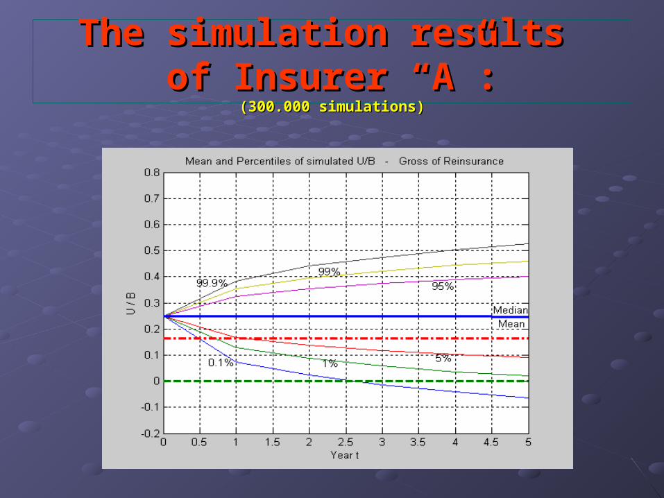
The simulation results The simulation results of Insurer “A”:of Insurer “A”:

(300.000 simulations)(300.000 simulations)

Simulation Moments of Simulation Moments of capital ratio U/B and loss ratio X/P:capital ratio U/B and loss ratio X/P:

SIMULATION MOMENTS OF THE CAPITAL RATIO U/B AND PURE LOSS RATIO X/P (% VALUES)

SIMULATION MOMENTS OF U/B SIMULATION MOMENTS OF X/P

t MEAN ST.DEV. SKEW. KURT. MEAN ST.DEV. SKEW. KURT.

0 25.00 100.000 - 1 24.94 4.82 - 0.26 3.43 99.998 6.41 + 0.25 3.43 2 24.88 6.60 - 0.18 3.25 99.993 6.37 + 0.28 3.70 3 24.82 7.82 - 0.15 3.15 100.001 6.30 + 0.26 3.68 4 24.78 8.73 - 0.13 3.12 99.983 6.24 + 0.24 3.32 5 24.73 9.45 - 0.11 3.10 99.999 6.17 + 0.23 3.31

Ruin ProbabilitiesRuin Probabilitieswith two different ruin barrierswith two different ruin barriers

% values% values

WITH RUIN BARRIER URUIN =0 WITH RUIN BARRIER URUIN=1/3*MSM

Time t

ANNUAL

RUIN PROB.

ONE-YEAR

RUIN PROB. FINITE TIME RUIN

PROB.

ANNUAL

RUIN

PROB.

ONE-YEAR

RUIN

PROB.

FINITE

TIME

RUIN

PROB.

1 0.01 0.01 0.01 0.05 0.05 0.05 2 0.05 0.04 0.05 0.31 0.28 0.33 3 0.16 0.13 0.18 0.87 0.68 1.01 4 0.36 0.25 0.44 1.60 1.03 2.05 5 0.61 0.38 0.81 2.33 1.19 3.27

A comparison of U/B Distribution (t =1 and 5):A comparison of U/B Distribution (t =1 and 5):uu00=25%, n=25%, n00=10.000, =10.000, σσqq=5%,=5%, u u00=25%, n=25%, n00=10.000, =10.000, σσqq=5%,=5%,

E(Z)=3.500, E(Z)=3.500, ccZZ=4 and =4 and λλ=1.8%=1.8% E(Z)=10.000, E(Z)=10.000, ccZZ=10 and =10 and λλ=5%=5%

Mean = 24.94 %Mean = 24.94 %Std = 4.82 %Std = 4.82 %Skew = - 0.26Skew = - 0.26

t=1

t=5


a



Effect of a 20% QS Reinsurance: Effect of a 20% QS Reinsurance: (with fixed reins. commission = 20% (with fixed reins. commission = 20%

unfavourable for the Insurer because exp=25%unfavourable for the Insurer because exp=25%):):

Gross of reins. Net of reins.

Effects on Effects on Finite Time Ruin Probability UFinite Time Ruin Probability Ureqreq/B/B00

Conf. level = 99.0%

Prof. Nino Savelli

Effects on Effects on UUreqreq/B/B00 with confidence levels 99.9% and 99.0% with confidence levels 99.9% and 99.0%

MINIMUM RISK CAPITAL REQUIRED FOR A DIFFERENT TIME HORIZON AS A PERCENT

VALUE OF THE INITIAL GROSS PREMIUMS (UREQ(0,T)/B0) ACCORDING TWO DIFFERENT

CONFIDENCE LEVELS GROSS OF REINS. NET OF REINS.

Time

Horizon T

CONFID. 99.9%

CONFID. 99.0%

UREQ(T) / UREQ(1)

CONFID. 99.9%

CONFID. 99.0%

UREQ(T) / UREQ(1)

T = 1 17.07 % 11.26 % 1.00 14.73 % 10.09 % 1.00 T = 2 22.31 % 15.17 % 1.35 20.07 % 14.36 % 1.42 T = 3 26.73 % 17.94 % 1.59 24.83 % 17.80 % 1.76 T = 4 30.27 % 20.43 % 1.81 28.94 % 21.07 % 2.09 T = 5 33.62 % 22.40 % 1.99 32.99 % 24.01 % 2.38

A comparison between A comparison between UUreqreq and EU MSM ? and EU MSM ?

Here are disregarded many sources of risk (as e.g. Here are disregarded many sources of risk (as e.g. claim reserving run-off, investment risk and claim reserving run-off, investment risk and underwriting cycles)underwriting cycles)

Here only a single-line Insurer is regarded (with a Here only a single-line Insurer is regarded (with a reduced variability – creduced variability – cZZ))

No dividends and taxation are assumed (but it does No dividends and taxation are assumed (but it does not affect so much the downside risk for the usual not affect so much the downside risk for the usual short time horizon used for solvency analyses). short time horizon used for solvency analyses).

Simulating a trade-off functionSimulating a trade-off function

Ruin Probability (or UES) vs Expected RoE can be figured Ruin Probability (or UES) vs Expected RoE can be figured out for all the reinsurance strategies available in the out for all the reinsurance strategies available in the market, with a minimum and a maximum constraint market, with a minimum and a maximum constraint

Minimum constraintMinimum constraint: Capital Return (e.g. E(RoE)> 5%): Capital Return (e.g. E(RoE)> 5%)Maximum constraintMaximum constraint: Risk of Default (e.g. PrRuin < 1%): Risk of Default (e.g. PrRuin < 1%)

Clearly both Risk and Performance measures will decrease Clearly both Risk and Performance measures will decrease as the Insurer reduces its risk retention, but as the Insurer reduces its risk retention, but treaty conditions treaty conditions (commissions and loadings mainly) are heavily affecting (commissions and loadings mainly) are heavily affecting the most efficient reinsurance strategy, as much as the the most efficient reinsurance strategy, as much as the above mentioned min/max constraintsabove mentioned min/max constraints..

Risk vs Profitability:Risk vs Profitability:(Ruin barrier = 0)(Ruin barrier = 0)

UES vs E(RoE)UES vs E(RoE) Ruin Prob. vs E(RoE)Ruin Prob. vs E(RoE)

Effects of Effects of other Reinsurance covers:other Reinsurance covers:

5% 5% Quota Share Quota Share

with cwith cRERE=22.5%=22.5%(instead of 20%)(instead of 20%)

XL XL

with kwith kMM=8 and =8 and

λλRERE=10.8%=10.8%

The effects on Risk and Profitability of The effects on Risk and Profitability of the three reinsurance covers:the three reinsurance covers:

under management constraints for T=3under management constraints for T=3

min(RoE)=25% and max(UES)=0.04 per millemin(RoE)=25% and max(UES)=0.04 per mille TIME

HORIZON NO REINSURANCE TREATY A:

20% QS AND CRE=20% TREATY B:

5% QS AND CRE=22.5% TREATY C:

XL AND RE=10.8%

T EXP. RETURN

UES(T) / BT

EXP. RETURN

UES(T) / BT

EXP. RETURN

UES(T) / BT

EXP. RETURN

UES(T) / BT

(0,T) (0,T) (0,T) (0,T) % ‰ % ‰ % ‰ % ‰

1 9.97 0.0064 4.28 0.0026 9.11 0.0050 8.18 0.0000 2 20.97 0.0228 8.77 0.0112 19.13 0.0182 17.07 0.0005 3 33.05 0.0584 13.45 0.0304 30.09 0.0455 26.84 0.0068 4 46.44 0.1259 18.42 0.0934 42.20 0.1024 37.42 0.0288 5 61.12 0.2253 23.56 0.2375 55.44 0.1930 49.03 0.0761

Part IIPart II

Multi-line Insurer

Introducing the Investment Risk (partly)

Introducing Taxation and Dividends

A larger Risk Loading on Premiums

An Insurer with 2 casualty lines:An Insurer with 2 casualty lines:Insurer “B”Insurer “B”

Line 1 as the (single-line) Insurer “A” (gross and net of reins.);Line 1 as the (single-line) Insurer “A” (gross and net of reins.);Line 2 (independent of line 1)Line 2 (independent of line 1) has a very small expected number of has a very small expected number of claims (n=100 and claims (n=100 and σσ(q)=25%(q)=25%) but with a large expectation and ) but with a large expectation and variability of the claim size (variability of the claim size (m=50.000 m=50.000 Eur and Eur and ccZZ=20=20) and a ) and a significant expected profitability (significant expected profitability (λλ=25%);=25%);Real growth rate: g=5%Real growth rate: g=5%Claim Inflation: i=5%;Claim Inflation: i=5%;Reinsurance cover for line 2: Reinsurance cover for line 2: QS 60% with fixed reins. comm. = 35% (< exp. loading = 40%);QS 60% with fixed reins. comm. = 35% (< exp. loading = 40%);

Total Premium Volume: Total Premium Volume: Eur 57,9 mln at year 1Eur 57,9 mln at year 1Eur 94,4 mln at year 5;Eur 94,4 mln at year 5;

Premium Mix (constant):Premium Mix (constant): 82.0% for line 1 82.0% for line 1 18.0% for line 218.0% for line 2

Retained Premium:Retained Premium: 72.8 %72.8 %Initial aggregate Capital Ratio (U/B):Initial aggregate Capital Ratio (U/B): 25.0 %25.0 %

INSURER BINSURER BCapital ratio U/B and Loss ratio X/PCapital ratio U/B and Loss ratio X/P

(gross reins.)(gross reins.) (net reins.)(net reins.)

An Insurer with 3 casualty lines:An Insurer with 3 casualty lines:Insurer “C”Insurer “C”

Lines 1 and 2 as the Insurer “B” (gross and net of reins.);Lines 1 and 2 as the Insurer “B” (gross and net of reins.);Line 3 (independent from both lines 1&2)Line 3 (independent from both lines 1&2) has n=2.500 (with has n=2.500 (with σσ(q)=5%) (q)=5%) and exp. claim size m=2.000 Eur with size variability cand exp. claim size m=2.000 Eur with size variability cZZ=1. Safety =1. Safety loading loading λλ=5% and exp.loading=30%;=5% and exp.loading=30%;Real growth rate: g=5%Real growth rate: g=5% Claim Inflation: i=5%;Claim Inflation: i=5%;Reinsurance cover for line 3: Reinsurance cover for line 3: QS 10% with fixed reins. comm. = exp. loading = 30%;QS 10% with fixed reins. comm. = exp. loading = 30%;

Total Premium Volume: Total Premium Volume: Eur 65,4 mln at year 1Eur 65,4 mln at year 1Eur 106.6 mln at year 5;Eur 106.6 mln at year 5;

Premium Mix (constant):Premium Mix (constant): 72.6% for line 1 72.6% for line 1 15.9% for line 215.9% for line 2 11.5% for line 311.5% for line 3

Retained Premium:Retained Premium: 74.8 % 74.8 % Initial aggregate Capital Ratio (U/B):Initial aggregate Capital Ratio (U/B): 25.0 %. 25.0 %.

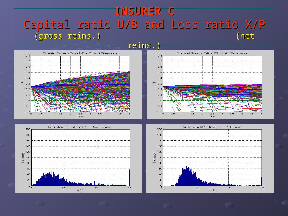
INSURER CINSURER CCapital ratio U/B and Loss ratio X/PCapital ratio U/B and Loss ratio X/P

(gross reins.)(gross reins.) (net reins.)(net reins.)

Comparison among Insurers A/B/C: Comparison among Insurers A/B/C: Min. Capital Ratio Required uMin. Capital Ratio Required ureqreq

MAIN ASSUMPTIONS:MAIN ASSUMPTIONS:

no claim reserving riskno claim reserving risk

no Investment riskno Investment risk

no correlation among lines of bus.no correlation among lines of bus.

no premium cyclesno premium cycles

no dividendsno dividends

no taxation no taxation

Insurer A

Insurer B Insurer C

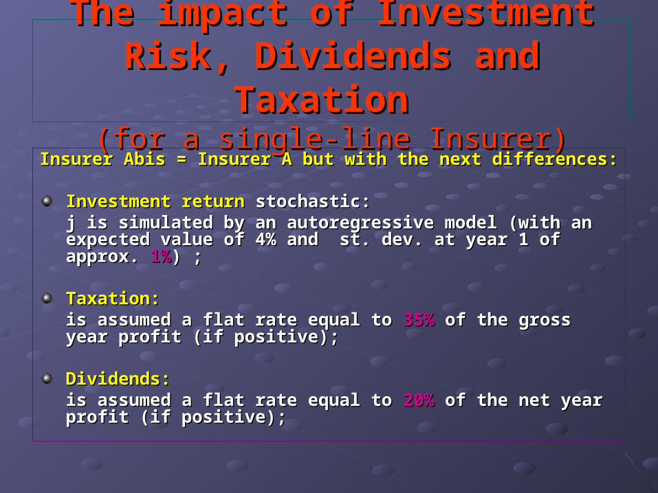
The impact of Investment Risk, The impact of Investment Risk, Dividends and Taxation Dividends and Taxation

(for a single-line Insurer)(for a single-line Insurer)Insurer Abis = Insurer A but with the next differences:Insurer Abis = Insurer A but with the next differences:

Investment returnInvestment return stochastic: stochastic: j is simulated by an autoregressive model (with an expected j is simulated by an autoregressive model (with an expected value of 4% and st. dev. at year 1 of approx. value of 4% and st. dev. at year 1 of approx. 1%1%) ;) ;

Taxation: Taxation: is assumed a flat rate equal to is assumed a flat rate equal to 35% 35% of the gross year profit (if of the gross year profit (if positive);positive);

Dividends: Dividends: is assumed a flat rate equal to is assumed a flat rate equal to 20%20% of the net year profit (if of the net year profit (if positive);positive);

INSURER AINSURER A INSURER AbisINSURER AbisCapital ratio u=U/BCapital ratio u=U/B

Insurer A – gross reins.

Insurer A – net reins.

Insurer Abis – gross reins.

Insurer Abis – net reins.

Comparison Insurers A and Abis: Comparison Insurers A and Abis: Min. Capital Ratio Required uMin. Capital Ratio Required ureqreq

MAIN ASSUMPTIONS:MAIN ASSUMPTIONS:


no Investment riskno Investment risk



no dividendsno dividends

no taxation no taxation


yes Investment riskyes Investment risk



yes dividendsyes dividends

yes taxationyes taxation

Insurer A

Insurer BInsurer A bis

Comparison Insurers A and Abis: Comparison Insurers A and Abis: some commentssome comments

The presence of the The presence of the Investment riskInvestment risk (here only partly (here only partly regarded because no claim reserve is assumed) implies regarded because no claim reserve is assumed) implies a slightly larger ua slightly larger ureqreq::e.g. for a confidence level 99.0%e.g. for a confidence level 99.0%uureqreq(1)=11.35% and u(1)=11.35% and ureqreq(2)= 15.37% (2)= 15.37% 11.26% and 15.17% (if j=4%=const.) 11.26% and 15.17% (if j=4%=const.)

for the Insurer here regarded for the Insurer here regarded TaxationTaxation (35%) and (35%) and DividendsDividends (20%) do not have a significant impact on the (20%) do not have a significant impact on the downside risk and then on the solvency requirements;downside risk and then on the solvency requirements;e.g. for a confidence level 99.0%e.g. for a confidence level 99.0%uureqreq(1)=11.38% and u(1)=11.38% and ureqreq(2)= 15.44% (2)= 15.44% 11.26% and 15.17% (j=4% tx=div=0%) 11.26% and 15.17% (j=4% tx=div=0%)

The impact of The impact of Risk Loading on Premiums:Risk Loading on Premiums:

Insurer A λ=1.80% Insurer A λ=5.00%

Final CommentsFinal Comments

Final CommentsFinal Comments : :

The risk of insolvency is heavily affected by, among others, The risk of insolvency is heavily affected by, among others, the tail of the tail of Total Claims Amount distributionTotal Claims Amount distribution;;

Variability and skewness of some variables are extremely relevant: Variability and skewness of some variables are extremely relevant: structure variable, claim size variability, investment returnstructure variable, claim size variability, investment return, etc.;, etc.;

A natural choice to reduce risk and to get an efficient capital allocation A natural choice to reduce risk and to get an efficient capital allocation is to give a portion of the risks to reinsurers, possibly with a favorable is to give a portion of the risks to reinsurers, possibly with a favorable pricing. As expected, the results of simulations show how pricing. As expected, the results of simulations show how reinsurance is reinsurance is usually reducing not only the insolvency risk but also the expected usually reducing not only the insolvency risk but also the expected profitability of the companyprofitability of the company. . In some extreme cases, notwithstanding In some extreme cases, notwithstanding reinsurance, the insolvency risk may result larger because of an reinsurance, the insolvency risk may result larger because of an extremely expensive cost of the reinsurance coverage: that happens extremely expensive cost of the reinsurance coverage: that happens when the reinsurance price is incoherent with the structure of the when the reinsurance price is incoherent with the structure of the transferred risktransferred risk

In many cases the EU “Minimum Solvency Margin” is not In many cases the EU “Minimum Solvency Margin” is not reliablereliable and an unsuitable risk profile is reached also for a short and an unsuitable risk profile is reached also for a short time horizon (T≤2) in the results of simulations. It is to emphasize time horizon (T≤2) in the results of simulations. It is to emphasize that that in our simulations neither (appropriate) investment risk nor in our simulations neither (appropriate) investment risk nor claims reserve run-off risk have been considered;claims reserve run-off risk have been considered;

It is possible It is possible to define an efficient frontier for the trade-off to define an efficient frontier for the trade-off Insolvency Risk / Shareholders ReturnInsolvency Risk / Shareholders Return according different according different reinsurance treaties and different retentions according the available reinsurance treaties and different retentions according the available pricing in the market;pricing in the market;

Insurance Solvency II:Insurance Solvency II:

these simulation models may be used for defining New Rules for these simulation models may be used for defining New Rules for Capital Adequacy (also for consolidated requirements);Capital Adequacy (also for consolidated requirements);

A new approach of Supervising Authorities:A new approach of Supervising Authorities:

assessing the solvency profile of the Insurer according to more or assessing the solvency profile of the Insurer according to more or less favourable scenarios (different level of control) and to indicate less favourable scenarios (different level of control) and to indicate the appropriate measures in case of an excessive risk of insolvency the appropriate measures in case of an excessive risk of insolvency in the short-term. in the short-term.

An available measure for the Guarantee Funds:An available measure for the Guarantee Funds:

additional premiums related to the effective Insurer’s risk of additional premiums related to the effective Insurer’s risk of insolvencyinsolvency

Internal Risk Models: Internal Risk Models:

to be used not only for solvency purposes but also for to be used not only for solvency purposes but also for management’s strategies and rating;management’s strategies and rating;

Appointed Actuary: Appointed Actuary:

appropriate simulation models are useful for the role of the appropriate simulation models are useful for the role of the Appointed Actuary or similar figures in General Insurance (e.g. for Appointed Actuary or similar figures in General Insurance (e.g. for MTPL in Italy), in order to analyse the effect of the strategic triangle MTPL in Italy), in order to analyse the effect of the strategic triangle Pricing/Reserving/Reinsurance on the Solvency profile of the Pricing/Reserving/Reinsurance on the Solvency profile of the company.company.

IAS:IAS:

to measure in advance the effects of the main forthcoming IAS to measure in advance the effects of the main forthcoming IAS

Further Researches and Further Researches and Improvements of the Model:Improvements of the Model:

Run-Off dynamics of Claims Reserving;

Modelling Investment Risk;

Premium Rating and Premium CyclesPremium Cycles;

Dynamic dividends policy and taxation;

Correlation among different insurance lines (Copula analyses);

Comparison of different risk measures

Variable reinsurance commissions and profit/losses participation;

Financial Reinsurance and ART;

Asset allocation strategies and non-life ALM;

Modelling Catastrophe Losses;

Modelling a multiplayer market with high policyholders’ sensitivity to either premium measure and insurer’s financial strength, with special reference to TPML (Games Theory).

The impact of forthcoming IAS.

Main References :Main References :

Beard, PentikBeard, Pentikääinen, E.Pesonen (1969, 1977,1984)inen, E.Pesonen (1969, 1977,1984)BBüühlmann (1970)hlmann (1970)British Working Party on General Solvency (1987)British Working Party on General Solvency (1987)Bonsdorff et al. (1989)Bonsdorff et al. (1989)Daykin & Hey (1990)Daykin & Hey (1990)Daykin, PentikDaykin, Pentikääinen, M.Pesonen (1994)inen, M.Pesonen (1994)Taylor (1997)Taylor (1997)Klugman, Panjer, Willmot (1998)Klugman, Panjer, Willmot (1998)Coutts & Thomas (1998)Coutts & Thomas (1998)Cummins et al. (1998)Cummins et al. (1998)Savelli (2002 e 2003)Savelli (2002 e 2003)IAA Solvency Working party (2003)IAA Solvency Working party (2003)FSA (CP 190, 2003)FSA (CP 190, 2003)

management simulation models and solvency in general insurance ___________________ nino savelli...

Documents