managerial biases and corporate risk management - …chitru f_managerialbiases(2).pdf · managerial...
TRANSCRIPT
Managerial Biases and Corporate Risk Management∗
Tim R. Adam School of Business and Economics, Humboldt University of Berlin
Dorotheenstr. 1, 10117 Berlin, Germany Tel.: +49 / 30 2093 5641; Fax: 49 / 30 2093 5643
E-mail: [email protected]
Chitru S. Fernando Price College of Business, University of Oklahoma
307 West Brooks, Norman, OK 73019, USA Tel.: (405) 325-2906; Fax: (405) 325-7688
E-mail: [email protected]
Evgenia Golubeva Price College of Business, University of Oklahoma
307 West Brooks, Norman, OK 73019, USA Tel: (405) 325-7727; Fax: (405) 325-7688
E-mail: [email protected]
Abstract
We show that managerial behavioral biases, which have been found to influence a number of corporate financial decisions, also affect corporate risk management. We find that managers reduce their hedge positions when the market moves against a hedge, but do not systematically increase their hedge positions when the market moves in favor of the hedge. This asymmetric response is consistent with managerial loss aversion coupled with mental accounting, two behavioral biases that have been documented in other corporate contexts. Furthermore, we find that managers increase their speculative activities, measured by the volatility of hedge positions, following speculative gains, but do not reduce their speculative activities following speculative losses. This finding is consistent with managerial overconfidence. Our findings provide the first evidence that corporate risk management practices are affected by managerial behavioral biases, and suggest that recognizing the presence of these biases will help bridge the gap between the theory and practice of corporate risk management.
This version: July 14, 2010
JEL Classification: G11; G14; G32; G39 Keywords: corporate risk management; manager behavior; speculation; mental accounting; loss aversion; overconfidence.
∗ We thank Alex Butler, Sudheer Chava, Louis Ederington, Gary Emery, Dirk Jenter, Swami Kalpathy, Leonid Kogan, Shimon Kogan, Nan Li, Gustavo Manso, Bill Megginson, Darius Miller, Jun Pan, Roberto Rigobon, Martin Ruckes, Antoinette Schoar, Oliver Spalt, Per Stromberg, Rex Thomson, Pradeep Yadav, and seminar participants at MIT, University of Oklahoma, Humboldt University, University of Texas at Dallas, Southern Methodist University, Texas Christian University, ESMT Berlin, 2008 FMA Europe meetings, 2008 FMA meetings, 2009 EFA meetings and 2010 AFA meetings for valuable discussions and comments. We are grateful to Ted Reeve for providing us with his derivatives surveys of gold mining firms and Leung Kam Ming for excellent research assistance. We also thank Anthony May and Jesus Salas for valuable assistance. This research has been partially supported by the Research Grants Council of Hong Kong (Grant No. HKUST6138/02H). A part of this research was conducted when Chitru Fernando was a visiting professor at the SMU Cox School of Business. He thanks SMU for their gracious hospitality and the National Science Foundation (Grant No. ECS-0323620) for financial support. We are responsible for any remaining errors.
Managerial Biases and Corporate Risk Management
Abstract
We show that managerial behavioral biases, which have been found to influence a number of corporate financial decisions, also affect corporate risk management. We find that managers reduce their hedge positions when the market moves against a hedge, but do not systematically increase their hedge positions when the market moves in favor of the hedge. This asymmetric response is consistent with managerial loss aversion coupled with mental accounting, two behavioral biases that have been documented in other corporate contexts. Furthermore, we find that managers increase their speculative activities, measured by the volatility of hedge positions, following speculative gains, but do not reduce their speculative activities following speculative losses. This finding is consistent with managerial overconfidence. Our findings provide the first evidence that corporate risk management practices are affected by managerial behavioral biases, and suggest that recognizing the presence of these biases will help bridge the gap between the theory and practice of corporate risk management. JEL Classification: G11; G14; G32; G39 Keywords: corporate risk management; manager behavior; speculation; mental accounting; loss aversion; overconfidence.
1
For years, hedging made Southwest Airlines Co. the most consistently profitable airline in the U.S. But included in its third-quarter earnings, released Thursday, was a $247 million accounting charge, which reflected the decline in the value of its hedges as the price of oil dropped during the quarter. The charge caused Southwest, which had a healthy operating profit, to post a quarterly net loss for the first time in 17 years. “Southwest is looking for opportunities to "de-hedge" some of its fuel,” Gary Kelly, the airline's chief executive, said Thursday. "Low fuel prices are a good thing...and an opportunity that we'll want to take the best advantage of that we can." Wall Street Journal, “Fuel Hedges Cloud Airline Results,” October 17, 2008. “Ask any gambler - on the way up it’s all about skill, on the way down it’s damned bad luck.” Financial Times, “Southwest’s Loss,” October 16, 2008. 1. Introduction
The traditional theories of corporate risk management have derived conditions under which
managers who act rationally in the interest of shareholders can add value by reducing the effects
of market frictions, such as taxes, bankruptcy costs, agency costs, information asymmetries, and
undiversified stakeholders of the firm.1 However, empirical tests of the predictions of these
theories have met with only limited success.2 While individual empirical studies uncover
evidence that can be interpreted as being consistent with one or more of the theories of hedging,
there is little consistency across studies. In addition, much of the variation in firms’ derivatives
strategies, both cross-sectionally and over time, remains unexplained. This disparity between
theory and practice is remarkably consistent with an argument advanced nearly 50 years ago by
Working (1962), that the “traditional” risk avoidance notion of hedging – matching one risk with
an opposing risk – is deficient when it comes to explaining hedging behavior in practice. Indeed,
the growing evidence that many managers systematically incorporate their market views into
their risk management programs3 but fail to generate positive cash flows from this “selective
1 See, for example, Stultz (1984), Smith and Stultz (1985), Froot, Scharfstein and Stein (1993), DeMarzo and Duffie (1995), Leland (1998), Breeden and Viswanathan (1998) and Mello and Parsons (2000). 2 See, for example, Tufano (1996), Mian (1996), Geczy, Minton and Schrand (1997), Graham and Smith (1999), Haushalter (2000) and Graham and Rogers (2002). 3 See, for example, Dolde (1993), Stultz (1996), Bodnar, Hayt and Marston (1998), and Glaum (2002).

2
hedging” strategy4 provides support for the notion that managerial behavior can deviate from the
pure rationality assumed by the neoclassical theories of hedging.
In this paper, we study the risk management activities of a sample of North American
gold mining firms and present new evidence that lends strong support for behavioral
explanations of some practices associated with corporate hedging. A growing body of literature,
both theoretical and empirical, studies the impact of managerial behavioral biases on corporate
decisions.5 Several managerial biases, including loss aversion, mental accounting, and
overconfidence, have been found to affect corporate investment policies, capital structure
decisions, mergers and acquisitions, security offerings, and investment bank relationships.6 To
the best of our knowledge, ours is the first study to examine whether managerial behavioral
biases also affect corporate risk management decisions.
First, we find that managers tend to reduce their hedge positions when the market moves
against the hedge. The reaction is asymmetric: when the market moves in favor of the hedge,
managers do not systematically increase their hedge positions. This asymmetry is inconsistent
with the existing theories of hedging, but consistent with the presence of behavioral biases such
as loss aversion (Kahneman and Tversky (1979); Tversky and Kahneman (1991)) which implies
a higher sensitivity to losses than to gains of equal magnitude. For example, while oil prices were
rising, Southwest Airlines’ fuel hedging activities were regarded as state-of-the-art, but when oil
prices fell and the fuel hedges began to generate losses, Southwest Airlines moved swiftly to
unwind its hedge positions despite realizing offsetting gains from lower fuel prices. Similar to
4 See Adam and Fernando (2006) and Brown, Crabb and Haushalter (2006). 5 Baker, Ruback, and Wurgler (2007) provide a comprehensive review of the literature on behavioral corporate finance. 6 Studies include Roll (1986), Loughran and Ritter (2002), Heaton (2002), Ljungqvist and Wilhelm (2005), Malmendier and Tate (2005, 2008), Ben-David, Graham and Harvey (2007), Billett and Qian (2008), Goel and Thakor (2008), Sautner and Weber (2009), and Gervais, Heaton and Odean (2009).
3
the case of Southwest Airlines, hedging losses in our sample of gold mining firms are offset by
gains in their underlying gold holdings. Yet, gold mining firms seem to treat these hedging losses
as “real” losses and react accordingly. A possible explanation for treating hedging losses as
“real” losses without regard to the gain in the underlying position arises from mental accounting.
The concept of mental accounting was first proposed by Thaler (1980, 1985) and summarized by
Grinblatt and Han (2005) as follows: “The main idea is that decision makers tend to segregate
different types of gambles into separate accounts … by ignoring possible interactions.” Thus,
mental accounting implies that managers regard losses on derivatives positions separately from
simultaneous gains on the underlying position. A risk management policy influenced by loss
aversion and mental accounting implies that managers will implement hedging strategies that
minimize derivatives losses. In contrast, to the extent rational theories of hedging imply an
asymmetric response to gold price movements, we would expect firms to respond more promptly
to downward gold price movements to protect against financial distress.
The second main finding of our paper is that managers tend to increase the level of their
speculative activities using derivatives, measured by the volatility of hedge positions, following
speculative gains, but do not reduce their speculative activities following speculative losses. This
asymmetric response, which persists after controlling for several firm characteristics, is again
difficult to reconcile with rational theories of risk management, but is consistent with the
presence of managerial overconfidence. The managerial overconfidence hypothesis (e.g., Heaton
(2002); Malmendier and Tate (2005, 2008)) implies that managers may be overconfident in their
ability to beat the market, engaging in excessive position shifting under the mistaken belief that
they have a relative information advantage. In particular, overconfidence is expected to increase
following successes, but decrease less (if at all) following failures. This asymmetric response
4
follows from selective self-attribution: successes tend to be attributed to one’s own skill, while
failures tend to be attributed to bad luck.
In summary, we document new evidence about the time-series properties of corporate
derivatives practices that is consistent with the possibility that managerial behavioral biases
affect derivatives strategies. Our findings are robust to numerous controls for alternative rational
explanations, and contribute to the growing literature on behavioral biases by showing that
managerial behavioral biases can also impact corporate risk management. Recognizing that
managers sometimes deviate from strict rationality is likely to improve our understanding of
corporate risk management decisions and help close the gap between the observed practice of
risk management and the extant neoclassical theory that seeks to explain it.
The remainder of the paper is organized as follows. Section 2 discusses the relevant
behavioral theories and derives testable hypotheses. Section 3 describes our sample, the
construction of our variables and the empirical methodology. Section 4 presents the empirical
evidence on how hedging responds to gold price changes. Section 5 presents the empirical
evidence on how speculation responds to speculative gains and losses. Section 6 summarizes the
results and presents our conclusions.
2. Empirical Hypotheses
The objective of this paper is to test whether managerial behavioral biases are likely to affect
corporate risk management decisions. As documented by Baker, Ruback, and Wurgler (2007) in
their excellent review of the growing literature on behavioral corporate finance, several
managerial behavioral biases have been shown to affect corporate decisions. We are
investigating the potential effects on corporate risk management decisions of three managerial
behavioral biases: mental accounting, loss aversion and overconfidence.
5
Mental accounting (Thaler (1980, 1985)) implies that managers maintain separate mental
accounts for different decision variables. Mental accounting may lead to sub-optimal decisions if
managers ignore the possible interdependencies of the decision variables when making decisions,
i.e., managers make decisions for each mental account separately. For example, Sautner and
Weber (2009) report that managers are more likely to sell shares acquired from exercising
options than shares acquired through required stock investments. This behavior is consistent with
mental accounting. Loughran and Ritter (2002) provide an explanation for IPO underpricing
based on mental accounting: managers do not mind underpricing as long as it is not larger than
the “gain” between the midpoint of the filing-price range and the first-day closing price.
Ljungqvist and Wilhelm (2005) show that behavioral factors can explain the likelihood that firms
will switch IPO underwriters for subsequent offerings and the fees that underwriters charge for
such offerings. Coleman (2007) uses an experimental survey setting to study managerial choices
over risky alternatives and finds evidence that the surveyed managers maintain separate mental
accounts for the consequences of decision outcomes and for the probabilities of those outcomes.
In the context of risk management, mental accounting implies that managers maintain one
account for derivatives-related gains and losses, and a separate account for the gains and losses
on the underlying asset. Thus, managers exhibiting mental accounting may make decisions
related to their derivatives portfolio while disregarding the gains/losses on the underlying asset.
The literature on cognitive biases ties mental accounting to another behavioral bias
known as loss aversion (Kahneman and Tversky (1979); Tversky and Kahneman (1991)). Loss
aversion implies that individuals are more sensitive to losses than they are to gains of equal
magnitude. That is, they exhibit non-standard utility functions.
6
Mental accounting coupled with loss aversion implies that individuals tend to be loss
averse over specific accounts rather than their overall position. For example, Barberis and Huang
(2001) argue that investors exhibit loss aversion over individual stocks in their portfolios rather
than over their overall portfolios. In the corporate risk management context, mental accounting
coupled with loss aversion implies that managers are more sensitive to derivatives losses than to
derivatives gains, and at least partially ignore any offsetting effects in the hedged positions.
Moreover, Tversky and Kahneman (1991) review considerable prior evidence which suggests
that managers who are loss averse will also react more intensely to losses than to gains by
moving to reverse actions that led to the loss (see also Thaler and Johnson (1990)). Therefore
managers who exhibit mental accounting and loss aversion will reduce their hedge positions
when they result in hedging losses, but will not systematically increase their hedge positions
when they result in hedging gains.7
Recent anecdotal evidence shows that, like in the aforementioned case of Southwest
Airlines, gold mining firms moved swiftly to cut or eliminate their hedges after losing money on
contracts due to rising gold prices. According to the Wall Street Journal (March 17, 2008), “last
year, in the largest cut since 2002, gold mining companies reduced their committed hedged
positions by 35%.” One prominent example is the de-hedging of Barrick Gold (Wall Street
Journal, July 28, 2004) when facing rising gold prices: “Barrick reduced its hedge position to
13.9 million ounces, down 850,000 ounces in the quarter,” which contributed to its 42% drop in
quarterly net income. We have uncovered no public announcements or other anecdotal evidence 7 Loss aversion has been commonly associated in the investments literature with a reluctance to sell losing investments, i.e., the disposition effect (Shefrin and Statman (1985)), which arises when the heightened sensitivity to losses generates an attempt to gamble out of a sure loss (unless the sensitivity to losses is itself dynamically affected by the loss, in which case the disposition effect may not obtain (Thaler and Johnson, (1990)). However, drawing a parallel to the disposition effect is not straightforward in the context of corporate hedging since one cannot clearly say that keeping a hedge open is more of a gamble than closing it out. Nonetheless, the basic premise of loss aversion – the higher sensitivity to losses than to gains of equal magnitude – implies that managers will more likely notice and act upon a derivatives loss associated with corporate hedging.

7
to suggest a similarly swift response when gold prices are moving downwards. In contrast, to the
extent rational theories of hedging imply an asymmetric response to gold price movements we
would expect firms to respond more promptly to downward gold price movements to protect
against financial distress.
Another managerial behavioral bias that has been widely documented in recent studies is
managerial overconfidence (see, for example, Russo and Schoemaker (1992), Griffin and
Tversky (1992) and Heaton (2002)). Overconfident managers systematically overestimate the
probability of good outcomes (and correspondingly, underestimate the probability of bad
outcomes) resulting from their actions (Heaton (2002)). In a dynamic setting, overconfidence
coupled with biased self-attribution (Miller and Ross (1975)), where managers credit themselves
for successes while blaming outside factors for failures, cause managerial overconfidence to
increase following successes but not commensurately decrease following failures (Daniel,
Hirshleifer and Subrahmanyam (1998); Gervais and Odean (2001)). The implications for
corporate financial decisions are that overconfident managers act more decisively and
aggressively, and that this behavior intensifies following successes. Several studies, including
Malmendier and Tate (2005, 2008), Ben-David, Graham and Harvey (2007), Billett and Qian
(2008), and Malmendier, Tate and Yan (2010), report empirical evidence consistent with
overconfident managers, while Barber and Odean (2000) report similar evidence in the context
of overconfident individual investors.
We test the overconfidence hypothesis in the context of corporate risk management.
There is ample evidence that managers incorporate their market views into their hedging
decisions, and thus hedge “selectively.”8 Adam and Fernando (2006) and Brown, Crabb and
8 See Dolde (1993), Stultz (1996), Bodnar, Hayt and Marston (1998), and Glaum (2002).
8
Haushalter (2006) document significant time-series variation in the size of the hedge positions of
gold mining firms, which may reflect managers’ changing market views about future gold prices.
In the absence of an information advantage with respect to gold prices, however, incorporating a
manager’s private market view into a hedging program is inconsistent with neoclassical theories
of risk management. Indeed, Adam and Fernando (2006) and Brown, Crabb and Haushalter
(2006) do not find systematic gains from selective hedging, which implies that managers of gold
mining firms do not possess an information advantage on average. Thus, the significant time-
series variation in firms’ hedge positions is likely to be inconsistent with rational explanations of
corporate hedging.
The managerial overconfidence hypothesis applied in the context of corporate speculation
implies that managers grow more overconfident following past speculative successes, leading to
a more aggressive pursuit of speculative strategies, while past failures would diminish managers’
willingness to speculate to a lesser degree, if at all. Hence, we expect an asymmetric relation
between speculative activities and the past performance of speculative positions, where managers
increase their speculative activities following successes in speculation, while they do not
commensurately decrease speculation following failures in speculation.
It could be argued that shareholders, rather than managers, are potentially affected by
some of the above behavioral biases and exert pressure on rational managers to react
asymmetrically. However, while shareholders observe gold price changes, they do not fully
observe dynamic hedging strategies or the resulting variation in derivatives cash flows.
Therefore, it is unlikely that shareholder pressure can fully underlie all our empirical hypotheses.
We discuss other alternative explanations in subsection 3.3 below.
9
Our mental accounting / loss aversion hypothesis predicts that managers will close out
hedges following losses while our overconfidence hypothesis predicts that they will speculate
more following past speculative success. These hypotheses may seem contradictory since in the
first case managers react sharply to “losses” while in the latter case they react sharply to “gains.”
Note, however, that a “speculative success” does not imply a “hedging gain” i.e., a drop in the
price of gold. Likewise, the act of speculation (dynamically varying derivatives positions in
response to changes in market views) does not imply a directional response of a hedge position
to a change in the price of gold. For example, a speculative contrarian manager and a speculative
momentum manager would react in opposite ways to the same price change. Therefore, the two
hypotheses test two quite independent behavioral phenomena.
3. Data and Methodology
3.1 Data and variables
Our sample consists of 92 gold mining firms in North America, which are included in the Gold
and Silver Hedge Outlook, a quarterly survey of derivatives activities conducted by Ted Reeve,
an analyst at Scotia McLeod, from 1989 through 1999, when he discontinued the survey.9 These
92 firms represent the majority of firms in the gold mining industry (see Tufano (1996) and
Adam and Fernando (2006)). Firms not included in the survey tend to be small or privately held
corporations.
The survey contains information on all outstanding gold derivatives positions, their size
and direction, maturities, and the respective delivery prices for each instrument (forwards, spot-
9 While some post-2000 hedging data is available from accounting disclosures and other sources, this data lacks the level of detail and consistency across firms that has made the Scotia McLeod survey data invaluable for many empirical studies of corporate hedging, including Tufano (1996, 1998), Fehle and Tsyplakov (2005), Adam and Fernando (2006), and Brown, Crabb and Haushalter (2006).
10
deferred contracts, gold loans and options). This derivatives data is described in detail in Adam
(2002). We hand-collect operational data: gold production (in ounces), production costs per
ounce of gold, and gold reserves, from firms’ annual reports. The data on firm characteristics
such as size, market-to-book, leverage, liquidity, existence of a credit rating, and payment of
quarterly dividends comes from Compustat. Data on managerial compensation is from
ExecuComp, supplemented by hand collection from proxy statements where necessary. All
variable notations and definitions are provided in Appendix 1.
We measure the extent of derivatives usage at a given point in time t with time to
maturity i by a hedge ratio HR(i)t, defined as follows:
]Prod[
)()(itt
tt E
iNiHR+
= , (1)
where N(i)t is the sum of the firm’s derivatives positions in place at time t (in ounces of gold)
that mature in i years, weighted by their respective deltas, as in Tufano (1996). Et[Prodt+i] is the
firms’s expectation of its gold production (in ounces of gold) at time t+i as of time t. The
maturity i of a derivatives position can be 1, 2, 3, 4, or 5 years, although most derivatives activity
takes place with contracts that mature within three years. To check robustness of our results we
aggregate (a) contracts with 1-3 years maturity and (b) contracts with 1-5 years maturity.
The derivatives survey reports the expected production for each hedge horizon i
whenever a firm has derivatives positions outstanding that mature in i years. If a firm does not
hedge a particular maturity, then the expected production figures are missing. In this case we use
the actual gold production in year t+i. Since most firms do not hedge their gold production
beyond three years, the problem of missing expected production figures increases with the hedge
horizon. Therefore, we also define an alternate hedge ratio, HRRes(i)t, that does not rely on
11
expected production but scales a firm’s total derivatives position by its total gold reserve (see Jin
and Jorion (2006)):
t
tt
iNiHRReserve Gold
)()(Res = . (2)
In addition to helping overcome potential issues associated with missing production data, scaling
by reserves is also a useful robustness check of our analysis using production-based hedge ratios,
due to the possibility that some time-series variation in the production-based hedge ratio may be
due to unplanned variations in expected production rather than a change in the firm’s derivatives
positions.
We observe the above hedge ratios every quarter from December 1989 to December
1999. This data allows us to measure the extent of speculation (selective hedging) by the time-
series volatility in hedge ratios. To obtain quarterly volatility estimates while also maximizing
the number of observations in our relatively small sample, we follow the existing literature on
volatility estimation and calculate volatility by the absolute change in a firm’s hedge ratio.
Alizadeh, Brandt, and Diebold (2002) review the large body of literature that estimates time-
varying volatility using two daily observations: either open and close, or high and low. They
argue, in particular, that the range, or the difference in log prices between daily high and daily
low, is a good proxy for daily volatility. To quote, “…the discretized stochastic volatility model
is difficult to estimate because the sample path of the asset price within each interval is not fully
observed…. In practice, we are forced to use discretely observed statistics of the sample paths,
such as the absolute or squared returns over each interval, to draw inferences about the
discretized log volatilities and their dynamics…” The measure advocated by Alizadeh et al.
(2002) has been used not only in market microstructure but also, for example, in asset pricing
research. Ang, Hodrick, Xing, and Zhang (2006) mention using the range-based volatility
12
measure as a proxy for innovations in aggregate market volatility, in order to estimate whether
exposure to these innovations is a priced risk.
Thus, we define the extent of speculation in quarter t, Vt, as the absolute value of the
difference in the natural logarithms of the hedge ratios at the beginning and the end of each
quarter.10
)]/([ 1−= ttt HRHRLNABSV (3)
This approach permits us to obtain quarterly volatility estimates, in contrast to (at best) annual
volatility estimates that we would obtain using the time-series standard deviation of hedge
ratios.11
We use several constructs to measure the past performance of firms’ derivatives
activities. First, we compute the quarterly total cash flows generated from derivatives positions
per ounce of gold hedged, as in Adam and Fernando (2006). Second, we recalculate the quarterly
cash flows assuming a firm had maintained a constant hedge ratio (“benchmark cash flows”).
The difference between the total derivatives cash flow and the cash flow computed using this
fixed hedge ratio benchmark is the cash flow that we attribute to selective hedging.12 Positive
selective hedging cash flows constitute “speculative gains” and negative selective hedging cash
flows constitute “speculative losses.” Selective hedging cash flow is an attractive measure
because it reflects the part of the cash flow that results directly from managerial market timing,
10 For the purpose of measuring percentage changes, whenever a firm reports a zero hedge (unless it reports a zero value in both the beginning and the end of the quarter), we substitute a very small value. The percentage change is then calculated as the difference of the natural logarithms from quarter (t-1) to quarter t. 11 An apparent refinement would be to estimate predicted hedge ratios as in Adam and Fernando (2006) and use the hedge ratio residuals to compute speculation. However, as demonstrated by Adam and Fernando (2006) in their robustness checks, speculation computed using hedge ratio residuals does not yield substantively different results to speculation computed using total hedge ratios, which may be due in part to the inability of fundamental variables to explain the variation in hedge ratios. 12 Adam and Fernando (2006) provide details on the computation of these cash flows.

13
i.e., speculative, actions.13 Finally, in addition to the above cash flow measures, we also calculate
the quarterly derivatives book profit (or loss), which is computed as the quarterly change in the
value of derivatives positions in dollars per ounce hedged. Please refer to Appendix 2 for the
calculation of quarterly changes in the book value of derivatives positions.
Tables 1 and 2 show the descriptive statistics and the correlations for the different hedge
ratios and hedge ratio volatility measures.
[Place Tables 1 & 2 about here]
Several observations emerge from these tables. Consistent with Adam and Fernando
(2006), selective hedging cash flows average at around zero, suggesting that selective hedging
does not add value to the firm on a systematic basis. We notice that the hedge ratios of different
maturities are all significantly correlated with one another. However, the correlations are weaker
between shorter-maturity and longer-maturity hedge ratios. The aggregate hedge ratios are less
than perfectly correlated with one another, substantiating the need to check robustness of our
results with respect to different hedge ratio definitions. The same general conclusions hold for
the hedge ratio volatilities.
3.2 Basic methodology
Our basic methodology is to run panel regressions with firm fixed effects in order to focus on the
time-series variation in hedge ratios. We estimate the loss aversion hypothesis on the whole
sample and, for robustness, on the subsample of firms that hedge in the sample period (i.e., have
at least one non-zero hedge ratio). We test our hypothesis on both groups of firms to avoid the
13 For example, suppose a manager believes that the gold price is going to rise and therefore reduces the hedge ratio relative to the benchmark. If she is correct in her forecast, then the total derivatives cash flow will be negative (since she is short overall) but the selective component will be positive: the firm does not lose as much on the hedge as it could have.
14
possibility that sample selection bias could affect the results for the subsample of hedgers and
because we do not know ex ante that non-hedgers will persist in not hedging throughout our
sample period. Keeping non-hedgers in the sample will make a finding in support of the loss
aversion hypothesis less likely, ex post. A firm that has a zero hedge ratio will not reduce the
hedge ratio in response to a gold price increase. At the same time, a firm that has a zero hedge
ratio may increase the hedge ratio in response to a gold price decrease. Therefore, by keeping
non-hedgers in the sample we decrease (increase) the unconditional probability of observing a
significant reaction to increases (decreases) in the price of gold, which would work against the
loss aversion hypothesis. We then check the robustness of our results by taking non-hedgers out
of the sample.
In our initial tests, we estimate the sensitivity of the hedge ratio to past changes in the
price of gold while controlling for firm characteristics that may affect the fundamental hedging
needs of the firm, as well as seasonal dummies and a time trend. Subsequently, we consider the
possibility that the initial level of the hedge ratio may affect the firm’s reaction to the gold price
change.
For robustness we repeat our tests using the two-step Heckman (1979) procedure with
selection. In the first stage, we model the existence of hedging activity as a function of variables
that are predicted by extant hedging theory to be determinants of hedging -- firm size, market-to-
book ratio, liquidity, leverage, dividend payment, credit rating, and the likelihood of financial
distress (Tufano (1996), Haushalter (2000)). We say that a firm has hedging activity if two
conditions hold: (1) the beginning or the end-of-quarter hedge ratio is non-zero; and (2) cash
flows from derivatives positions in the previous quarter are non-zero. In the second stage of the
Heckman two-step procedure, we test whether the hedge ratio is sensitive to past changes in the

15
price of gold for the firms that exhibit hedging activity as described above. Further
methodological details are provided in Section 4.
Our test of managerial overconfidence, which is based on the relationship between hedge
ratio volatility and past speculative gains and losses, needs to be restricted to active hedgers only
(i.e., firms that have non-zero hedge ratios and report non-zero cash flows in the previous
period). This requirement is due to the fact that the overconfidence hypothesis conditions
managerial activity on the results of previous activity. In addition, leaving non-hedging firm-
quarters in the sample may lead to a spurious regression result with zero past cash flows from
derivatives positions “explaining” zero hedge ratio volatility next period. Hence, we estimate the
panel regression with firm fixed effects on a reduced sample of active hedgers. As in our
previous tests, for robustness we repeat our overconfidence tests using the two-step Heckman
(1979) procedure with selection. The first stage of the Heckman two-step procedure is described
above. In the second stage we test whether the hedge ratio volatility is driven by past success of
the derivatives positions for the firms that exhibit hedging activity as described above. Further
methodological details are provided in Section 5.
Our unique data permits us to employ a methodology that is distinct from and
complements the techniques employed in the other studies of corporate managerial biases.
Existing studies fall under two categories: surveys, as in Ben-David, Graham, and Harvey
(2007); and cross-sectional studies, as in Malmendier and Tate (2005). These studies examine a
variety of characteristics that are likely to affect the degree to which managers exhibit behavioral
biases. Examples include personal and professional characteristics (age, tenure, education, etc.)
and personal wealth management practices (the tendency to hold disproportionate amounts of
one’s own firm’s stock, and the failure to exercise vested options). The question in these studies
16
is whether cross-sectional differences across managers explain actions that are attributable to
behavioral biases. Our work complements the prior studies by focusing on time-series patterns
that may characterize behavioral biases, examining how managers as a group respond to market
movements and their own past performance. As noted before, this complementary perspective is
made possible by our unique data set, which contains quarterly observations on all outstanding
gold derivatives positions of a sample of 92 North American gold mining firms from 1989-1999.
The key advantage of this data set is that we are able to infer actual derivatives transactions and
the corresponding cash flows as well as observe the estimates of expected production, which is a
unique feature of our data set.
3.3 Controlling for alternative explanations
An alternative explanation for closing out losing derivatives positions may be liquidity pressure
or financial distress (Mello and Parsons (2000)). In particular, if a firm had insufficient liquidity
or be otherwise financially constrained, it is possible that managers may be forced to close out
losing positions due to margin calls. Therefore, we control for a firm’s liquidity and likelihood of
financial distress to allow for this possibility by including a dividend dummy, rating dummy,
quick ratio, leverage and Altman’s (1968) Z-score as control variables.
A second alternative explanation for the propensity to close out losing positions is the
possibility that book losses draw more scrutiny than book profits. We control for this possibility
by including derivatives book profits and losses in our regressions.14
14 The FAS 133 accounting standard, which made a significant departure from past accounting practice by requiring derivatives contracts to be marked to market, could also potentially affect the way managers react to market movements. However, our findings are unlikely to be affected by this change since our sample ends around the same time FAS 133 went into effect (in mid-1999).
17
An alternative explanation for an increase in speculation following high derivatives cash
flows derived from speculation is that managers simply have more cash to use at their discretion
or that positive cash flows from speculation improve the firm’s financial strength. We control for
a firm’s liquidity and financial strength to account for this possibility.15
Another possibility is that although selective hedging does not benefit shareholders, it
may benefit managers due to incentive compensation (Stulz (1996)). While the potential link
between selective hedging and managerial compensation is explored in several recent studies, the
results are mixed, with only weak evidence that managerial compensation significantly affects
selective hedging and no consensus on the direction of the relationship.16 Nevertheless, we
control for managerial compensation variables to allow for this possibility in our hedging
sample.
Finally, as pointed out by Campbell and Kracaw (1999), financially constrained firms
with good projects may speculate more to generate more funds for optimal investment.
Investment opportunities may also affect the degree to which firms choose to hedge due to the
need to raise external financing (Froot, Scharfstein and Stein (1993)). We account for both
financial constraints and growth opportunities by including standard control variables such as
debt-to-equity and market-to-book ratios.
15 It is important to note, however, that in contrast to positive speculative cash flows from derivatives, positive total derivatives cash flow need not make the overall financial position of the firm stronger because positive hedge cash flows on derivatives positions would typically offset losses due to gold price declines. 16 Géczy, Minton and Schrand (2007) find that CEO stock price sensitivity is negatively related to speculation while CFO stock price sensitivity is positively related. Beber and Fabbri (2006) find no consistent relation between CEO delta and selective hedging. Brown, Crabb and Haushalter (2006) find no systematic relationship between selective hedging and several ownership and compensation measures.
18
4. Empirical Results: Hedging Response to Gold Price Changes
In this section, we test the loss aversion hypothesis, which predicts that managers systematically
reduce their hedge positions when they produce hedging losses but do not systematically
increase their hedge positions when they produce hedging gains. Initially, we test this hypothesis
by examining how the change in the hedge ratio is related to the previous quarter’s change in the
gold price, while allowing for asymmetry effects and controlling for relevant firm characteristics.
Thereafter, we repeat our tests while allowing for the possibility that the relation between hedge
ratio changes and gold price changes may be affected by the initial level of the hedge ratio. We
conclude by carrying out robustness checks.
4.1 Initial tests
We begin with a simple question: Does the hedge ratio respond to past changes in the price of
gold? We normalize past changes in the price of gold by the initial gold price level, thereby
making gold returns our main independent variable of interest:
RTNGOLDt-1 = ∆GOLDt-2,t-1/GOLDt-2, (4)
since a given dollar change in the price of gold is likely to be perceived differently depending on
the prevailing gold price level.17
Table 3 reports the results of the regression:
tttt CONTROLSRTNGOLDbaHR ε++⋅+=Δ −− 11 (5)
17 While we report regression results that employ gold return as the independent variable, we also repeated our tests using dollar changes in the price of gold. The results of those tests are available upon request and are similar to the results obtained using gold returns.
19
We control for past changes in firm characteristics which may also explain a hedge ratio
adjustment following a change in the gold price. As our control variables, we choose the change
in size, liquidity (quick ratio), leverage, market-to-book, Altman’s Z-score, dividend dummy,
and credit rating dummy, to accommodate the possibility that a change in the price of gold may
change the fundamental hedging needs of the firm, or cause liquidity pressure and financial
distress. In addition, we control for seasonal variation using seasonal dummies, clustering of
some observations across quarters, and a time trend. The time trend is a variable equal to zero for
the first sample observation (December of 1989) and increasing by 0.25 each quarter. Finally, in
Models (3), (6), (9), and (12), we report the results obtained on a reduced sample with non-
hedgers (i.e. firms reporting a zero hedge ratio for the entire sample period) excluded from the
sample.
[Place Table 3 about here]
The evidence in Table 3 suggests that firms adjust hedge ratios in response to changes in
the price of gold, and that this adjustment occurs primarily for short hedge horizons. The
coefficient is highly significant, both statistically and economically, for the one-year hedge ratio.
A one standard deviation (5.27%) increase in the price of gold makes the average firm reduce its
one-year hedge ratio by about ten percent relative to the sample mean. For the aggregate three-
year and five-year hedge ratios, the gold return coefficient is smaller in magnitude and
sometimes insignificant, although the sign is still negative.18 Overall, the results indicate that
gold price changes affect hedging decisions.
We also notice that hedge ratios respond to changes in liquidity and that this effect too
occurs at short horizons. A reduction in the quick ratio, which indicates a decrease in liquidity, 18 Our finding of especially strong results when we use the short-term hedge ratio (i.e., up to one-year maturity), is consistent with prior studies showing that hedgers are more active in the shorter-term maturities (see, for example, Bodnar, Hayt and Marston, 1998).
20
makes the firm reduce its one-year hedge positions, and vice versa. However, the long-term
hedge positions appear to be unaffected by liquidity changes.
The main hypothesis tested in this section is that the response of hedge ratio to gold price
is asymmetrically stronger for gold price increases. Forcing an equal response to gold price
increases and decreases in our regression specification (5) does not allow for this effect to show.
Therefore, we next run the following regression to capture any asymmetric response:
ttttt CONTROLSIRTNGOLDbIRTNGOLDbaHR ε++⋅⋅+⋅⋅+=Δ −−− 1212111 (6)
In this regression, I1 is a dummy variable that equals one if the change in the gold price during
the last quarter was positive, and equals zero otherwise; and I2 is a dummy variable that equals
one if the change in the price of gold was negative, and equals zero otherwise. The sensitivity of
hedge ratios to gold price increases is determined by b1, while the sensitivity to gold price
decreases is determined by b2.
The results, presented in Table 4, are striking. In every model, regardless of the hedge
ratio specification and presence of control variables, the coefficient b1 is strongly negative and
statistically significant. At the same time, the coefficient b2 is always statistically insignificant.
That is, increases in the price of gold are followed by significant de-hedging while decreases in
the price of gold are not followed by a systematic increase in hedging. This result is robust to the
inclusion of changes in firm characteristics that may affect the firm’s hedging needs. The result
is also economically significant. A one standard deviation (5.27%) percentage increase in the
price of gold leads to a reduction of around 17 percent in the one-year hedge ratio relative to its
sample mean, with the magnitude of the reaction diminishing with the hedging horizon. Finally,
we continue to observe that at short horizons, hedge ratio adjustments are sensitive to variations
21
in liquidity. Once again, Models (3), (6), (9), and (12) present the results obtained on a reduced
sample with non-hedgers excluded.
[Place Table 4 about here]
4.2 Effect of initial hedge ratio
We next allow for the changes in hedge ratio to be affected by the initial hedge ratio. If a firm
has a low hedge ratio or does not hedge, the subsequent change in the hedge ratio is likely to be
positive, all else equal. A non-hedger may either remain a non-hedger or decide to start hedging,
thus making the hedge ratio adjustment positive, on average, for such firms. In addition, firms
with very low levels of hedge ratios are more likely to under-hedge, thereby increasing the
likelihood of a subsequent increase in hedging. Following the same logic, a firm with a very high
level of hedging is more likely to reduce its hedge ratio, all else equal. Hence, we expect to
observe a negative relationship, all else equal, between the initial level of hedge ratio and the
subsequent change. In other words, we can posit a systematic negative impact of the initial hedge
ratio on the subsequent change, which exists irrespective of changes in the price of gold or other
factors. In this section, we test whether our earlier results are robust to the inclusion of this
permanent impact into the regression. We re-run regression (6) with one more term added to the
specification:
tttttt HRcCONTROLSIRTNGOLDbIRTNGOLDbaHR ε+⋅++⋅⋅+⋅⋅+=Δ −−−− 11212111 (7)
In (7), HRt-1 is the beginning-of-quarter level of the hedge ratio. We expect the coefficient c to be
negative. We also expect the coefficient b1 to be negative and b2 to be zero, consistent with the
results reported in Table 4.
22
Table 5 presents the results of our regression (7) with firm characteristics, seasonal
dummies, and a time trend used as controls, as in Table 4. For additional robustness, models (3),
(6), (9), and (12) in Table 5 report the regression results on the reduced sample with non-hedgers
excluded. We can see that our hypothesis regarding the systematic effect of the initial level of
hedge ratio is confirmed: the coefficient for HRt-1 is universally negative and strongly significant.
We observe a marked improvement in the model fit as evidenced by the increase in R2 compared
to those reported in Table 4. Therefore, including the initial level of hedge ratio in the regression
is important for modeling hedging adjustments of firms. At the same time, our inference
regarding the effect of changes in the price of gold remains virtually unaffected. The coefficient
b1 is still negative and significant: a one standard deviation (5.27%) percentage increase in the
price of gold leads to a 10 percent reduction in the one-year hedge ratio relative to the sample
mean, with economic significance diminishing with hedging horizon as before. This result
indicates that firms robustly reduce their hedge ratios in response to increases in the price of
gold. At the same time, we observe no response to decreases in the price of gold: the coefficient
b2 remains insignificant in all specifications.
[Place Table 5 about here]
As an additional robustness check, we control for the possibility of selection bias in our
sample by allowing for the two sequential decisions of the firm, (1) whether or not to be a hedger
and (2) conditional on being a hedger, the choice of the level of hedging. We estimate the two-
step Heckman procedure with selection. In the first stage, we estimate a PROBIT model, where
the dependent variable is the “hedging activity” dummy equal to zero if (1) either the firm has
zero hedge ratios in both the beginning and the end of quarter t; or (2) the firm had zero cash

23
flows from hedging operations in quarter t-1.19 We estimate the likelihood of hedging activity as
a function of several firm characteristics: size, market-to-book ratio, the ratio of book debt to
book equity, quick ratio, dividend-payer status, existence of a credit rating, and Altman’s Z-
score. In the second stage, we estimate the relationship between the changes in hedge ratio and
past changes in the price of gold conditional on the firm being an active hedger.
The results from the two stages of the Heckman procedure are presented in Tables 6 and
7, respectively. From Table 6, we observe that firms that exhibit hedging activity are large firms
with low growth opportunities (as indicated by low market-to-book ratios), conservative leverage
policies, and higher financial constraints/low liquidity. These results are consistent with the
previously reported findings by Geczy, Minton and Schrand (1997), Bodnar, Hayt and Marston
(1998) and Haushalter (2000).
[Place Table 6 about here]
Table 7 presents the Heckman second-stage results. The results reported in Table 7 are
consistent with our previous findings reported in Table 5. We continue to observe a negative
relationship between changes in hedge ratio and past changes in the price of gold only when
those changes were positive, and the relationship is the strongest for the short-horizon hedge
ratio. We observe no relationship between changes in hedge ratio and past decreases in the price
of gold. As before, the initial level of the hedge ratio is negative and significant across all
hedging horizons.
[Place Table 7 about here]
19 We also run the first stage estimation using only the first condition (non-zero hedge ratios) to define hedging activity and obtain similar results. They are not reported due to space constraints but are available on request.
24
4.3 Controlling for alternative explanations
As mentioned in Section 3.3, in all our specifications we control for alternative explanations
based on extant hedging theories that may help explain firms’ hedge ratio adjustments following
gold price changes. In particular, we control for firm characteristics such as liquidity and
financial distress using a firm’s quick ratio, leverage, Altman’s Z-score, dividend dummy, and
credit rating dummy. These additional controls do not affect our principal results in any of the
specifications that we employ. We also include these variables in a non-linear fashion, for
example, by including the interaction of the change in liquidity with the change in gold price.
These additional tests do not affect our findings either and are available upon request. As
mentioned previously, we repeat all our tests using the dollar change in the price of gold in place
of gold return, with robust results. Finally, our results are robust to including the gold dummy as
a separate independent variable, to allow for the intercept term to vary with the direction of gold
price change.
5. Empirical Evidence: Speculation Response to Speculative Gains and Losses
In this section, we test the managerial overconfidence hypothesis by examining the relation
between speculation (measured by hedge ratio volatility) and past speculative gains and losses.
The overconfidence hypothesis maintains that, all else equal, if past speculative activity was
successful, resulting in cash flow gains, then the manager will increase his/her speculative
activities in the next period. If, however, past speculative activity was unsuccessful, resulting in
cash flow losses, then there would be no commensurate reduction in speculative activities. In
other words, we expect an asymmetric relation between the degree of speculative activity and
past speculative cash flows.
25
5.1 Initial panel regression without asymmetry effects
We begin by examining the general relationship between derivatives cash flows and subsequent
speculative activity. Tables 8 and 9 show the results of the firm fixed effects panel regressions of
the hedge ratio volatility on past cash flows and book profits from derivatives positions per
ounce of gold hedged. Similar to Table 3, we present the results for the volatility of the one-year
hedge ratio, the three-year aggregate hedge ratio scaled by expected production, the three-year
aggregate hedge ratio scaled by reserves, and the five-year hedge ratio scaled by reserves. Table
8 reports the results for a specification that employs total derivatives cash flows along with
derivatives book profit as independent variables. Our interest in this specification is to
investigate whether speculative activity responds to past derivatives cash flows and/or book
profits. Table 9 reports the corresponding results using selective hedging cash flows (i.e., the
speculative component of total derivatives cash flows), which is our primary variable of interest.
[Place Tables 8 and 9 about here]
Since we are interested in testing the hypothesis that successful past speculative
derivatives activity will lead to higher speculation in the future, we perform these regressions
after eliminating firm quarters where the firm had zero cash flows from derivatives positions,
and also eliminating observations where both beginning-of-quarter and end-of-quarter hedge
ratios were zero. In all of the models, we include seasonal dummy variables as controls;
however, doing so is mostly a concern with the one-year hedge ratio, which exhibits some
seasonal variation, whereas the aggregate hedge ratios exhibit virtually no seasonal variation. As
discussed in Section 3.3, we also control for firm characteristics that may affect a firm’s level of
speculative activity, such as liquidity, financial strength, and growth opportunities.

26
As evident from Table 8, we observe a positive relationship between hedge ratio
volatility and previous quarter total derivatives cash flows, which is robust to model specification
in terms of both magnitude and statistical significance. However, we do not observe any
relationship with the book profit. This result indicates that speculation responds to derivatives
cash flows but not to book profits. We then refine the specification to employ the selective
hedging component of derivatives cash flows. From Table 9, we observe that the relationship
between hedge ratio volatility and selective hedging cash flows is positive and significant,
providing evidence in favor of the hypothesis that the success of past selective hedging leads to
higher levels of speculation in the future. Again, we do not find a significant relationship with
book profits. Nonetheless, speculation is also positively related to benchmark cash flows, which
is consistent with our observation in Table 8 for total derivatives cash flows.
Given that the tests reported in Tables 8 and 9 were performed on a reduced sample, we
next perform robustness checks to control for the possibility of selection bias by allowing for the
two sequential decisions of the firm, (1) whether or not to be a hedger and (2) conditional on
being a hedger, how much to speculate. We estimate the two-step Heckman procedure with
selection. The first stage is the same PROBIT model described above in Section 4.2 and
presented in Table 6. In the second stage, we estimate the relationship between hedge ratio
volatility and past cash flows and book profits from derivatives positions conditional on the firm
being an active hedger.
Table 10 presents the Heckman second-stage results. The results reported in Table 10 are
consistent with our previous findings reported in Tables 8 and 9. In all regression specifications,
we observe a positive and significant relationship between hedge ratio volatility and past cash
flows from derivatives positions, whether total derivatives cash flows or selective hedging cash
27
flows and benchmark cash flows. We observe no relationship between hedge ratio volatility and
past book profits from derivatives positions.
[Place Table 10 about here]
We next perform one more robustness check to control for managerial compensation as
discussed in Section 3.3. Tables 11 and 12 present the results of the regressions of hedge ratio
volatility on past cash flows while controlling for the managerial compensation variables (delta
and vega) of the CEO and the CFO. The regressions are univariate due to the limited number of
managerial compensation observations in our sample. However, the regressions indicate that
overall, our inference regarding the effect of derivatives cash flows on speculation remains
unaffected while the managerial compensation variables are statistically insignificant.
[Place Tables 11 and 12 about here]
5.2 Accounting for asymmetry effects
Having established the relation between speculation and derivatives cash flows, we now turn to
our test for the presence of managerial overconfidence in our sample firms. We do so by
examining the asymmetry in the relationship between derivatives cash flows and speculation. For
this purpose, we run the following regression with dummy variables:
ttttt CONTROLSISCFbISCFbaV ε++⋅+⋅+= −− 212111 (8)
In this regression, I1 (I2) is a dummy variable that equals one if the selective hedging cash flow
during the last quarter was positive (negative) and zero otherwise. We choose selective hedging
cash flow to be the dependent variable because selective hedging cash flow is the direct
consequence of speculative decisions made by the manager in the past, and therefore is more
directly related to the extent to which past speculation was successful than total cash flows. We
28
include the benchmark cash flow, along with the firm characteristics, in the matrix of control
variables.20
We estimate this regression first on a reduced sample of firm-quarters for active hedgers
and next, using the Heckman two-step procedure for robustness. The results of the panel
regressions on the reduced sample are presented in Table 13, and the results of the second-stage
Heckman procedure with controls are presented in Table 14. While the asymmetric response of
hedge ratio volatility to selective cash flow persists in this alternative specification, the
significance of the benchmark cash flow variable is diminished.
[Place Tables 13 & 14 about here]
From both Table 12 and Table 13, we observe that the relationship between hedge ratio
volatility and past selective hedging cash flows is strongly positive only if the past selective
hedging cash flows are positive. A one-standard deviation increase in selective hedging cash
flow leads to a 0.2774 increase in the quarterly volatility of the one-year hedge ratio, which is
22.5% of the sample mean of 1.2325. When selective hedging cash flows are negative, however,
we observe no significant relationship except in the case of one-year hedge ratio volatility.
However, while we would still expect a positive coefficient for one-year hedge ratio volatility
with negative selective hedging cash flows if the relation between speculation and selective
hedging cash flow is symmetric (since speculation should decrease as speculation losses
increase) this is the opposite of what we observe for one-year hedge ratio volatility. Thus, our
evidence here strongly supports an asymmetric relation between speculative activity and
selective hedging cash flows, which confirms the managerial overconfidence hypothesis for our
sample firms. Managers increase speculative activity following successes (as their
20 Nevertheless, we check robustness of the results to using total derivatives cash flow and find that the general result is similar in spirit although less significant. The results are not reported but are available upon request.

29
overconfidence rises) but do not symmetrically reduce it following failures. This result is robust
to the inclusion of firm characteristics that may affect the fundamental hedging needs of the firm,
as well as to controlling for possible selection biases.
5.3 Other robustness checks
In addition to controlling for the rational explanations as laid out in Section 3.3, we also perform
a few more robustness checks. First, past cash flows as well as derivatives book profits may be
related to movements in the price of gold over the same quarter. This concern is mitigated by the
fact that derivatives cash flows are the result of hedging decisions taken in the distant past as
well as more current decisions and therefore, the recent change in the price of gold may not have
a strong effect. Additionally, this issue is much less of a concern for selective hedging cash
flows, which is our main variable of interest. Nevertheless, in unreported tests we include the
change in the price of gold in our regressions without a substantive effect on our results. In the
two-stage Heckman framework, we also allow for the relationship between hedge ratio volatility
and past selective hedging cash flows to be a function of the beginning-of-quarter hedge ratio. In
these robustness tests, also available upon request, we continue to find that hedge ratio volatility
is positively related to past derivatives cash flows and that the relationship is robustly stronger
for positive selective hedging cash flows, consistent with our managerial overconfidence
hypothesis.
6. Conclusions
We add to the growing body of literature that documents the presence of managerial behavioral
biases in a variety of corporate finance settings, including investment and capital structure

30
policy, mergers and acquisitions, security offerings and investment bank relationships, by
showing that the effect of these behavioral biases also extends to corporate hedging decisions.
We study how firms change their hedge positions in response to past changes in the gold price
and past performance of their hedging portfolios, using a 10-year sample of North American
gold mining firms that has been widely studied in the literature. Consistent with anecdotal
evidence, we find that managers systematically decrease their hedge positions following past
increases in the gold price, while they do not systematically increase their hedges following past
gold price declines. We interpret this evidence as consistent with managerial loss aversion and
mental accounting, i.e., managers act to minimize losses from derivatives positions, while paying
less regard to the performance of the underlying position. We also document a positive
relationship between speculation and past speculative gains, without a corresponding relation
between speculation and past speculative losses. This asymmetry supports the conjecture that the
financial success of past hedging decisions increases managerial overconfidence, leading
managers to elevate their levels of speculation. Our findings provide the first evidence that
corporate risk management practices are affected by managerial behavioral biases, and suggest
that recognizing the presence of these biases will help bridge the gap between the theory and
practice of corporate risk management.
31
Appendix 1: Variable Notations and Definitions
Hedge Ratios:
HR1 – HR5 are the hedge ratios from one- to five-year maturities, respectively;
A3 is the aggregate hedge ratio that aggregates the hedge positions over one-, two-, and three-
year horizons, scaled by the expected production;
A3R is the aggregate hedge ratio that aggregates the hedge positions over one-, two-, and three-
year horizons, scaled by gold reserves;
A5R is the aggregate hedge ratio that aggregates the hedge positions over one-, two-, three-,
four- and five-year horizons, scaled by gold reserves.
Hedge Ratio Volatility:
V1 – V5 are the quarterly volatilities of the one- through five-year hedge ratios, respectively.
Quarterly volatility is the absolute value of the difference in the natural logarithms of the end-of-
quarter and beginning-of-quarter hedge ratio levels.
V6 – V8 are the corresponding quarterly volatilities for A3, A3R, and A5R, respectively.
Derivatives Cash Flows:
CF are the total cash flows from derivatives positions (in $ per ounce hedged) estimated as in
Adam and Fernando (2006);
SCF and BCF are the selective and the benchmark cash flows, estimated as in Adam and
Fernando (2006);
RBK is the change in the book value of the derivatives positions per ounce hedged (see
Appendix 2).
Firm Characteristics:
SIZ is the logarithm of the market value of assets ($ million);

32
MB is the market-to-book ratio of assets;
DE is the ratio of book debt to book equity;
QCK is the quick ratio;
DIV is a dummy variable equal to one if the firm paid quarterly dividend;
RAT is a dummy variable equal to one if a firm reports a credit rating;
Z is the Altman’s (1968) Z-score (higher value of Z corresponds to lower probability of
bankruptcy).
DELTA_CEO (CFO) is the change in the dollar value of the CEO’s (CFO’s) wealth derived
from ownership of stock and stock options in the firm when the firm’s stock price changes by
one percent, calculated according to the methodology of Core and Guay (2002). We calculate the
aggregate delta of the executive’s compensation as the sum of the deltas of the options holdings
and the delta of the stock holdings.
VEGA_CEO (CFO) is the change in the dollar value of the CEO’s (CFO’s) wealth derived
from ownership of stock and stock options in the firm when the annualized standard deviation of
the firm’s stock price changes by 0.01, following Core and Guay (2002). We calculate the
aggregate vega of the executive’s compensation as the sum of the vegas of the executive’s
options holdings, following Coles, Daniel and Naveen (2006).
GLD is the change in the price of gold over the quarter;
33
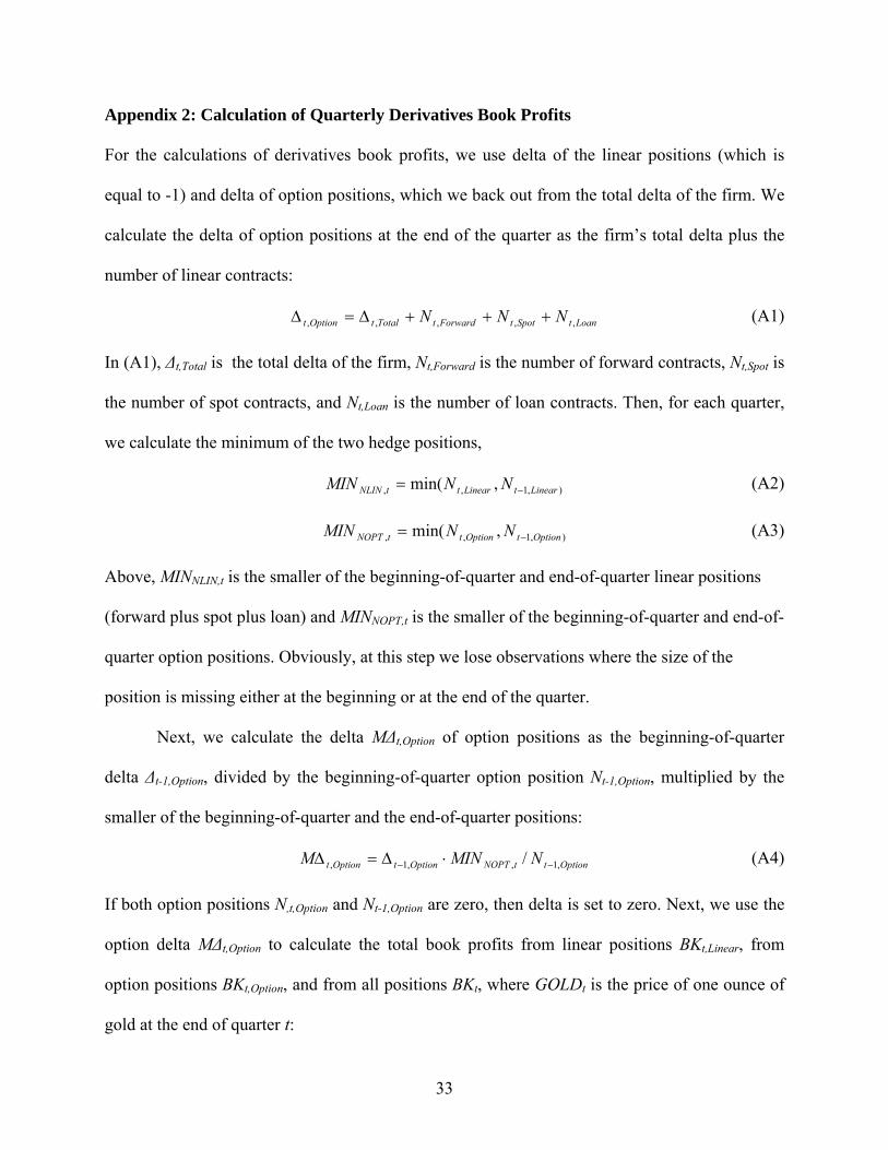
Appendix 2: Calculation of Quarterly Derivatives Book Profits For the calculations of derivatives book profits, we use delta of the linear positions (which is
equal to -1) and delta of option positions, which we back out from the total delta of the firm. We
calculate the delta of option positions at the end of the quarter as the firm’s total delta plus the
number of linear contracts:
LoantSpottForwardtTotaltOptiont NNN ,,,,, +++Δ=Δ (A1)
In (A1), Δt,Total is the total delta of the firm, Nt,Forward is the number of forward contracts, Nt,Spot is
the number of spot contracts, and Nt,Loan is the number of loan contracts. Then, for each quarter,
we calculate the minimum of the two hedge positions,
),1,, ,min( LineartLinearttNLIN NNMIN −= (A2)
),1,, ,min( OptiontOptionttNOPT NNMIN −= (A3)
Above, MINNLIN,t is the smaller of the beginning-of-quarter and end-of-quarter linear positions
(forward plus spot plus loan) and MINNOPT,t is the smaller of the beginning-of-quarter and end-of-
quarter option positions. Obviously, at this step we lose observations where the size of the
position is missing either at the beginning or at the end of the quarter.
Next, we calculate the delta MΔt,Option of option positions as the beginning-of-quarter
delta Δt-1,Option, divided by the beginning-of-quarter option position Nt-1,Option, multiplied by the
smaller of the beginning-of-quarter and the end-of-quarter positions:
OptionttNOPTOptiontOptiont NMINM ,1,,1, / −− ⋅Δ=Δ (A4)
If both option positions N,t,Option and Nt-1,Option are zero, then delta is set to zero. Next, we use the
option delta MΔt,Option to calculate the total book profits from linear positions BKt,Linear, from
option positions BKt,Option, and from all positions BKt, where GOLDt is the price of one ounce of
gold at the end of quarter t:
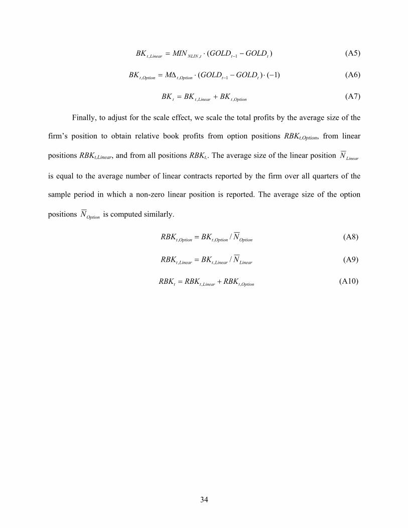
34
)( 1,, tttNLINLineart GOLDGOLDMINBK −⋅= − (A5)
)1()( 1,, −⋅−⋅Δ= − ttOptiontOptiont GOLDGOLDMBK (A6)
OptiontLineartt BKBKBK ,, += (A7)
Finally, to adjust for the scale effect, we scale the total profits by the average size of the
firm’s position to obtain relative book profits from option positions RBKt,Option, from linear
positions RBKt,Linear, and from all positions RBKt,. The average size of the linear position LinearN
is equal to the average number of linear contracts reported by the firm over all quarters of the
sample period in which a non-zero linear position is reported. The average size of the option
positions OptionN is computed similarly.
OptionOptiontOptiont NBKRBK /,, = (A8)
LinearLineartLineart NBKRBK /,, = (A9)
OptiontLineartt RBKRBKRBK ,, += (A10)
35
References Adam, Tim, 2002, Do Firms Use Derivatives to Reduce their Dependence on External Capital Markets? European Finance Review 6, 163-187. Adam, Tim, and Chitru Fernando, 2006, Hedging, Speculation, and Shareholder Value, Journal of Financial Economics 81, 283-309. Alizadeh, Sassan, Michael W. Brandt, and Francis X. Diebold, 2002, Range-Based Estimation of Stochastic Volatility Models, Journal of Finance 57, 1047-1092. Altman, Edward I., 1968, Financial Ratios, Discriminant Analysis and the Prediction of Corporate Bankruptcy, Journal of Finance 23, 589-609. Ang, Andrew, Robert J. Hodrick, Yuhang Xing, and Xiaoyan Zhang, 2006, The Cross-Section of Volatility and Expected Returns, Journal of Finance 61, 259-299. Baker, Malcolm, Richard S. Ruback, and Jeffrey Wurgler, 2007, Behavioral Corporate Finance: A Survey, in The Handbook of Corporate Finance: Empirical Corporate Finance, edited by Espen Eckbo. Elsevier/North Holland, New York. Barber, Brad M., and Terrance Odean, 2000, Trading is Hazardous to Your Wealth: The Common Stock Investment Performance of Individual Investors, Journal of Finance 55, 773-806. Barberis, Nicholas, and Ming Huang, 2001, Mental Accounting, Loss Aversion, and Individual Stock Returns, Journal of Finance 56, 1247-1292. Beber, Alessandro, and Daniela Fabbri, 2006, Who Times the Foreign Exchange Market? Corporate Speculation and CEO Characteristics, Working Paper. Ben-David, Itzhak, John R. Graham, and Campbell R. Harvey, 2007, Managerial Overconfidence and Corporate Policies, Working Paper. Billett, Matthew T., and Yiming Qian, 2008, Are Overconfident CEOs Born or Made? Evidence of Self-Attribution Bias from Frequent Acquirers, Management Science 54, 1037-1051. Bodnar, Gordon N., Gregory S. Hayt, and Richard C. Marston, 1998, Wharton Survey of Derivatives Usage by U.S. Non-Financial Firms, Financial Management 27, 70-91. Breeden, Douglas, and S. Viswanathan, 1998, Why Do Firms Hedge? An Asymmetric Information Model, Working Paper. Brown, Gregory W., Peter R. Crabb, and David Haushalter, 2006, Are Firms Successful at Selective Hedging? Journal of Business, 79, 2925-2949.
36
Campbell, Tim S. and William A. Kracaw, 1999, Optimal Speculation in the Presence of Costly External Financing. In “Corporate Risk: Strategies and Management,” Gregory Brown and Donald Chew, editors, Risk Publications, London. Coleman, Les, 2007, Risk and Decision Making by Finance Executives: A Survey Study, International Journal of Managerial Finance 1, 108-124. Daniel, Kent D., David Hirshleifer, and Avanidhar Subrahmanyam, 1998, Investor Psychology and Security Market Under- and Over-Reactions, Journal of Finance 53, 1839 – 1867. DeMarzo, Peter M. and Darrell Duffie, 1995, Corporate Incentives for Hedging and Hedge Accounting, Review of Financial Studies 8, 743 – 772. Dolde, Walter, 1993, The Trajectory of Corporate Financial Risk Management, Journal of Applied Corporate Finance 6, 33-41. Fehle, Frank, and Sergey Tsyplakov, 2005, Dynamic Risk Management: Theory and Evidence, Journal of Financial Economics 78, 3-47. Froot, Kenneth.A., David S. Scharfstein, and Jeremy C. Stein, 1993, Risk Management: Coordinating Corporate Investment and Financing Policies, Journal of Finance 48, 1629 – 1658. Géczy, Christopher C., Bernadette A. Minton, and Catherine Schrand, 1997, Why Firms Use Currency Derivatives, Journal of Finance 52, 1323-1354. Géczy, Christopher C., Bernadette A. Minton, and Catherine Schrand, 2007, Taking a View: Corporate Speculation, Governance and Compensation, Journal of Finance 62, 2405 – 2443. Gervais, Simon, J.B. Heaton, and Terrance Odean, 2009, Overconfidence, Compensation Contracts and Labor Markets, Working Paper. Gervais, Simon, and Terrance Odean, 2001, Learning to be Overconfident, Review of Financial Studies 14, 1-27. Glaum, Martin, 2002, The Determinants of Selective Exchange-Risk Management – Evidence from German Non-Financial Corporations, Journal of Applied Corporate Finance 14, 108 - 121. Goel, Anand, and Anjan Thakor, 2008, Overconfidence, CEO Selection and Corporate Governance, Journal of Finance 63, 2737- 2784. Griffin, Dale and Amos Tversky, 1992, The Weighing of Evidence and the Determinants of Confidence, Cognitive Psychology 24, 411-435. Grinblatt, Mark, and Bing Han, 2005, Prospect Theory, Mental Accounting, and Momentum, Journal of Financial Economics 78, 311-339.
37
Haushalter, G. David, 2000, Financing Policy, Basis Risk, and Corporate Hedging: Evidence from Oil and Gas Producers, Journal of Finance 55, 107 – 152. Heaton, J.B., 2002, Managerial Optimism and Corporate Finance, Financial Management, Summer, 33-45. Heckman, James J., 1979, Sample Selection as a Specification Error, Econometrica 47, 153 – 161. Jin, Yanbo, and Philippe Jorion, 2006, Firm Value and Hedging: Evidence from U.S. Oil and Gas Producers, Journal of Finance 61, 893 – 919. Kahneman, Daniel, and Amos Tversky, 1979, Prospect Theory: An Analysis of Decisions under Risk, Econometrica 47, 313-327. Leland, Hayne E., 1998, Agency Costs, Risk Management, and Capital Structure, Journal of Finance 53, 1213-1243. Ljungqvist, Alexander, and William J. Wilhelm, Jr., 2005, Does Prospect Theory Explain IPO Market Behavior? Journal of Finance 60, 1759-1790. Loughran, Tim, and Jay R. Ritter, 2002, Why Don’t Issuers Get Upset About Leaving Money on the Table in IPOs? Review of Financial Studies 15, 413-443. Malmendier, Ulrike, and Geoffrey Tate, 2005, CEO Overconfidence and Corporate Investment, Journal of Finance 60, 2661 – 2700. Malmendier, Ulrike, and Geoffrey Tate, 2008, Who Makes Acquisitions? CEO Overconfidence and the Market’s Reaction, Journal of Financial Economics 89, 20-43. Malmendier, Ulrike, Geoffrey Tate, and Jon Yan, 2010, Managerial Beliefs and Corporate Financial Policies, Working Paper. Mello, Antonio, and John Parsons, 2000, Hedging and Liquidity, Review of Financial Studies 13, 127 – 153. Miller, Dale T., and Michael Ross, 1975, Self-Serving Biases in the Attribution of Causality: Fact or Fiction? Psychological Bulletin 82, 213-225. Roll, Richard, 1986, The Hubris Hypothesis of Corporate Takeovers, Journal of Business 59, 197–216. Russo, J. Edward, and Paul J.H. Schoemaker, 1992, Managing Overconfidence, Sloan Management Review 33, 7–17.

38
Sautner, Zacharias, and Martin Weber, 2009, How Do Managers Behave in Stock Option Plans? Clinical Evidence from Exercise and Survey Data, Journal of Financial Research 32, 123-155. Shefrin, Hersh, and Meir Statman, 1985, The disposition to sell winners too early and ride losers too long: Theory and evidence, Journal of Finance 40, 777 – 790. Smith, Clifford W., and Rene M. Stulz, 1985, The Determinants of Firms’ Hedging Policies, Journal of Financial and Quantitative Analysis 20, 391-405. Stulz, René M., 1984, Optimal Hedging Policies, Journal of Financial and Quantitative Analysis 19, 127 – 140. Stulz, René M., 1996, Rethinking Risk Management, Journal of Applied Corporate Finance 9, 8-24. Thaler, Richard H., 1980, Towards a Positive Theory of Consumer Choice, Journal of Economic Behavior and Organization 1, 39-60. Thaler, Richard H., 1985, Mental Accounting and Consumer Choice, Marketing Science 4, 199-214. Thaler, Richard H., and Eric J. Johnson, 1990, Gambling with the House Money and Trying To Break Even: The Effects of Prior Outcomes on Risky Choice, Management Science 36, 643-660. Tufano, Peter, 1996, Who Manages Risk? An Empirical Examination of Risk Management Practices in the Gold Mining Industry, Journal of Finance 51, 1097-1137. Tufano, Peter, 1998. The Determinants of Stock Price Exposure: Financial Engineering and the Gold Mining Industry, Journal of Finance 53, 1051-1052. Tversky, Amos, and Daniel Kahneman, 1991, Loss Aversion in Riskless Choice: A Reference-Dependent Model, Quarterly Journal of Economics 106, 1039-1061. Working, Holbrook, 1962, New Concepts Concerning Futures Markets and Prices, American Economic Review 52, 431 – 459.
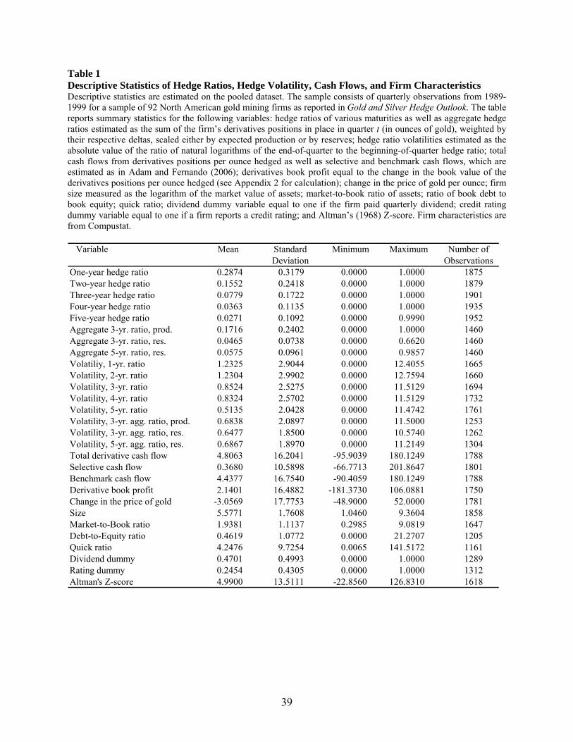
39
Table 1 Descriptive Statistics of Hedge Ratios, Hedge Volatility, Cash Flows, and Firm Characteristics Descriptive statistics are estimated on the pooled dataset. The sample consists of quarterly observations from 1989-1999 for a sample of 92 North American gold mining firms as reported in Gold and Silver Hedge Outlook. The table reports summary statistics for the following variables: hedge ratios of various maturities as well as aggregate hedge ratios estimated as the sum of the firm’s derivatives positions in place in quarter t (in ounces of gold), weighted by their respective deltas, scaled either by expected production or by reserves; hedge ratio volatilities estimated as the absolute value of the ratio of natural logarithms of the end-of-quarter to the beginning-of-quarter hedge ratio; total cash flows from derivatives positions per ounce hedged as well as selective and benchmark cash flows, which are estimated as in Adam and Fernando (2006); derivatives book profit equal to the change in the book value of the derivatives positions per ounce hedged (see Appendix 2 for calculation); change in the price of gold per ounce; firm size measured as the logarithm of the market value of assets; market-to-book ratio of assets; ratio of book debt to book equity; quick ratio; dividend dummy variable equal to one if the firm paid quarterly dividend; credit rating dummy variable equal to one if a firm reports a credit rating; and Altman’s (1968) Z-score. Firm characteristics are from Compustat.
Variable
One-year hedge ratio 0.2874 0.3179 0.0000 1.0000 1875Two-year hedge ratio 0.1552 0.2418 0.0000 1.0000 1879Three-year hedge ratio 0.0779 0.1722 0.0000 1.0000 1901Four-year hedge ratio 0.0363 0.1135 0.0000 1.0000 1935Five-year hedge ratio 0.0271 0.1092 0.0000 0.9990 1952Aggregate 3-yr. ratio, prod. 0.1716 0.2402 0.0000 1.0000 1460Aggregate 3-yr. ratio, res. 0.0465 0.0738 0.0000 0.6620 1460Aggregate 5-yr. ratio, res. 0.0575 0.0961 0.0000 0.9857 1460Volatiliy, 1-yr. ratio 1.2325 2.9044 0.0000 12.4055 1665Volatility, 2-yr. ratio 1.2304 2.9902 0.0000 12.7594 1660Volatility, 3-yr. ratio 0.8524 2.5275 0.0000 11.5129 1694Volatility, 4-yr. ratio 0.8324 2.5702 0.0000 11.5129 1732Volatility, 5-yr. ratio 0.5135 2.0428 0.0000 11.4742 1761Volatility, 3-yr. agg. ratio, prod. 0.6838 2.0897 0.0000 11.5000 1253Volatility, 3-yr. agg. ratio, res. 0.6477 1.8500 0.0000 10.5740 1262Volatility, 5-yr. agg. ratio, res. 0.6867 1.8970 0.0000 11.2149 1304Total derivative cash flow 4.8063 16.2041 -95.9039 180.1249 1788Selective cash flow 0.3680 10.5898 -66.7713 201.8647 1801Benchmark cash flow 4.4377 16.7540 -90.4059 180.1249 1788Derivative book profit 2.1401 16.4882 -181.3730 106.0881 1750Change in the price of gold -3.0569 17.7753 -48.9000 52.0000 1781Size 5.5771 1.7608 1.0460 9.3604 1858Market-to-Book ratio 1.9381 1.1137 0.2985 9.0819 1647Debt-to-Equity ratio 0.4619 1.0772 0.0000 21.2707 1205Quick ratio 4.2476 9.7254 0.0065 141.5172 1161Dividend dummy 0.4701 0.4993 0.0000 1.0000 1289Rating dummy 0.2454 0.4305 0.0000 1.0000 1312Altman's Z-score 4.9900 13.5111 -22.8560 126.8310 1618
Number ofDeviation Observations
Mean Standard Minimum Maximum
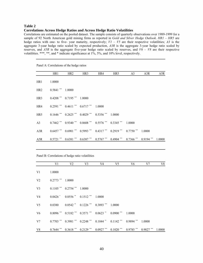
40
Table 2 Correlations Across Hedge Ratios and Across Hedge Ratio Volatilities Correlations are estimated on the pooled dataset. The sample consists of quarterly observations over 1989-1999 for a sample of 92 North American gold mining firms as reported in Gold and Silver Hedge Outlook. HR1 – HR5 are hedge ratios with one- to five- year maturity, respectively; V1 – V5 are their respective volatilities; A3 is the aggregate 3-year hedge ratio scaled by expected production, A3R is the aggregate 3-year hedge ratio scaled by reserves, and A5R is the aggregate five-year hedge ratio scaled by reserves, and V6 – V8 are their respective volatilities. ***, **, and * indicate significance at 1%, 5%, and 10% level, respectively.
Panel A: Correlations of the hedge ratios
HR1 HR2 HR3 HR4 HR5 A3 A3R A5R
HR1 1.0000
HR2 0.5841 *** 1.0000
HR3 0.4208 *** 0.7195 *** 1.0000
HR4 0.2591 *** 0.4611 *** 0.6717 *** 1.0000
HR5 0.1646 *** 0.2625 *** 0.4029 *** 0.5356 *** 1.0000
A3 0.7462 *** 0.9340 *** 0.8608 *** 0.5576 *** 0.3345 *** 1.0000
A3R 0.6457 *** 0.6901 *** 0.5993 *** 0.4317 *** 0.2919 *** 0.7750 *** 1.0000
A5R 0.5721 *** 0.6381 *** 0.6387 *** 0.5767 *** 0.4904 *** 0.7366 *** 0.9194 *** 1.0000
Panel B: Correlations of hedge ratio volatilities
V1 V2 V3 V4 V5 V6 V7 V8
V1 1.0000
V2 0.2773 *** 1.0000
V3 0.1105 *** 0.2754 *** 1.0000
V4 0.0426 * 0.0556 ** 0.1512 *** 1.0000
V5 0.0380 0.0542 ** 0.1226 *** 0.3893 *** 1.0000
V6 0.8096 *** 0.5182 *** 0.3571 *** 0.0623 ** 0.0900 *** 1.0000
V7 0.7703 *** 0.3981 *** 0.2248 *** 0.1044 ** 0.1142 *** 0.9894 *** 1.0000
V8 0.7644 *** 0.3618 *** 0.2129 *** 0.0927 *** 0.1020 *** 0.9785 *** 0.9827 *** 1.0000
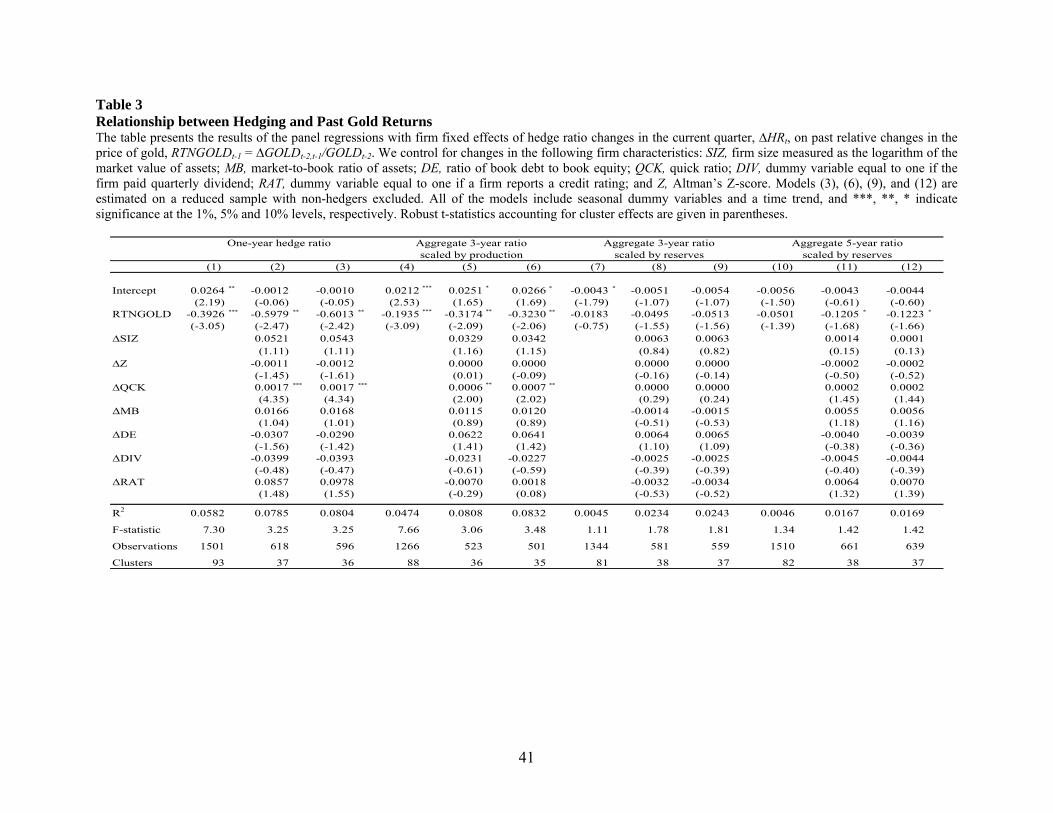
41
Table 3 Relationship between Hedging and Past Gold Returns The table presents the results of the panel regressions with firm fixed effects of hedge ratio changes in the current quarter, ∆HRt, on past relative changes in the price of gold, RTNGOLDt-1 = ∆GOLDt-2,t-1/GOLDt-2. We control for changes in the following firm characteristics: SIZ, firm size measured as the logarithm of the market value of assets; MB, market-to-book ratio of assets; DE, ratio of book debt to book equity; QCK, quick ratio; DIV, dummy variable equal to one if the firm paid quarterly dividend; RAT, dummy variable equal to one if a firm reports a credit rating; and Z, Altman’s Z-score. Models (3), (6), (9), and (12) are estimated on a reduced sample with non-hedgers excluded. All of the models include seasonal dummy variables and a time trend, and ***, **, * indicate significance at the 1%, 5% and 10% levels, respectively. Robust t-statistics accounting for cluster effects are given in parentheses.
Intercept 0.0264 ** -0.0012 -0.0010 0.0212 *** 0.0251 * 0.0266 * -0.0043 * -0.0051 -0.0054 -0.0056 -0.0043 -0.0044(2.19) (-0.06) (-0.05) (2.53) (1.65) (1.69) (-1.79) (-1.07) (-1.07) (-1.50) (-0.61) (-0.60)
RTNGOLD -0.3926 *** -0.5979 ** -0.6013 ** -0.1935 *** -0.3174 ** -0.3230 ** -0.0183 -0.0495 -0.0513 -0.0501 -0.1205 * -0.1223 *
(-3.05) (-2.47) (-2.42) (-3.09) (-2.09) (-2.06) (-0.75) (-1.55) (-1.56) (-1.39) (-1.68) (-1.66)∆SIZ 0.0521 0.0543 0.0329 0.0342 0.0063 0.0063 0.0014 0.0001
(1.11) (1.11) (1.16) (1.15) (0.84) (0.82) (0.15) (0.13)∆Z -0.0011 -0.0012 0.0000 0.0000 0.0000 0.0000 -0.0002 -0.0002
(-1.45) (-1.61) (0.01) (-0.09) (-0.16) (-0.14) (-0.50) (-0.52)∆QCK 0.0017 *** 0.0017 *** 0.0006 ** 0.0007 ** 0.0000 0.0000 0.0002 0.0002
(4.35) (4.34) (2.00) (2.02) (0.29) (0.24) (1.45) (1.44)ΔMB 0.0166 0.0168 0.0115 0.0120 -0.0014 -0.0015 0.0055 0.0056
(1.04) (1.01) (0.89) (0.89) (-0.51) (-0.53) (1.18) (1.16)ΔDE -0.0307 -0.0290 0.0622 0.0641 0.0064 0.0065 -0.0040 -0.0039
(-1.56) (-1.42) (1.41) (1.42) (1.10) (1.09) (-0.38) (-0.36)ΔDIV -0.0399 -0.0393 -0.0231 -0.0227 -0.0025 -0.0025 -0.0045 -0.0044
(-0.48) (-0.47) (-0.61) (-0.59) (-0.39) (-0.39) (-0.40) (-0.39)ΔRAT 0.0857 0.0978 -0.0070 0.0018 -0.0032 -0.0034 0.0064 0.0070
(1.48) (1.55) (-0.29) (0.08) (-0.53) (-0.52) (1.32) (1.39)
R2 0.0582 0.0785 0.0804 0.0474 0.0808 0.0832 0.0045 0.0234 0.0243 0.0046 0.0167 0.0169
F-statistic 7.30 3.25 3.25 7.66 3.06 3.48 1.11 1.78 1.81 1.34 1.42 1.42
Observations 1501 618 596 1266 523 501 1344 581 559 1510 661 639
Clusters 93 37 36 88 36 35 81 38 37 82 38 37
scaled by production scaled by reservesscaled by reservesOne-year hedge ratio Aggregate 3-year ratio Aggregate 3-year ratio Aggregate 5-year ratio
(1) (4) (7) (10)(2) (3) (11) (12)(5) (6) (8) (9)
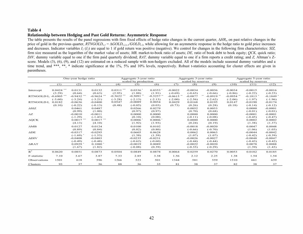
42
Table 4 Relationship between Hedging and Past Gold Returns: Asymmetric Response The table presents the results of the panel regressions with firm fixed effects of hedge ratio changes in the current quarter, ∆HRt, on past relative changes in the price of gold in the previous quarter, RTNGOLDt-1 = ∆GOLDt-2,t-1/GOLDt-2, while allowing for an asymmetric response in the hedge ratio to gold price increases and decreases. Indicator variables I1 (I2) are equal to 1 if gold return was positive (negative). We control for changes in the following firm characteristics: SIZ, firm size measured as the logarithm of the market value of assets; MB, market-to-book ratio of assets; DE, ratio of book debt to book equity; QCK, quick ratio; DIV, dummy variable equal to one if the firm paid quarterly dividend; RAT, dummy variable equal to one if a firm reports a credit rating; and Z, Altman’s Z-score. Models (3), (6), (9), and (12) are estimated on a reduced sample with non-hedgers excluded. All of the models include seasonal dummy variables and a time trend, and ***, **, * indicate significance at the 1%, 5% and 10% levels, respectively. Robust t-statistics accounting for cluster effects are given in parentheses.
Intercept 0.0424 *** 0.0131 0.0132 0.0311 *** 0.0336 * 0.0353 * -0.0022 -0.0034 -0.0036 -0.0034 -0.0015 -0.0016(3.29) (0.64) (0.63) (2.95) (1.88) (1.91) (-0.69) (-0.65) (-0.66) (-0.86) (-0.22) (-0.23)
RTNGOLD∙I1 -0.6905 *** -0.9432 *** -0.9624 *** -0.3622 *** -0.5091 ** -0.5257 ** -0.0615 ** -0.0877 ** -0.0919 ** -0.0954 ** -0.1813 * -0.1849 *
(-3.60) (-3.24) (-3.21) (-3.28) (-2.13) (-2.13) (-2.00) (-2.56) (-2.62) (-2.06) (-1.97) (-1.96)RTNGOLD∙I2 0.0182 -0.0636 -0.0400 0.0547 -0.0089 0.0054 0.0429 0.0168 0.0195 0.0147 -0.0190 -0.0174
(0.10) (-0.22) (-0.13) (0.48) (-0.05) (0.03) (0.73) (0.26) (0.28) (0.18) (-0.14) (-0.12)∆SIZ 0.0461 0.0487 0.0266 0.0279 0.0052 0.0053 0.0000 -0.0001
(0.99) (1.00) (0.97) (0.97) (0.70) (0.68) (-0.01) (-0.01)∆Z -0.0010 -0.0011 0.0000 0.0000 0.0000 0.0000 -0.0001 -0.0001
(-1.29) (-1.43) (0.10) (0.00) (-0.11) (-0.08) (-0.45) (-0.47)∆QCK 0.0017 *** 0.0017 *** 0.0006 * 0.0006 * 0.0000 0.0000 0.0002 0.0002
(4.13) (4.10) (1.92) (1.93) (0.24) (0.19) (1.38) (1.37)ΔMB 0.0127 0.0124 0.0100 0.0102 -0.0018 -0.0020 0.0047 0.0048
(0.89) (0.84) (0.82) (0.80) (-0.66) (-0.70) (1.06) (1.03)ΔDE -0.0317 -0.0295 0.0605 0.0628 0.0062 0.0063 -0.0044 -0.0042
(-1.69) * (-1.53) (1.38) (1.39) (1.07) (1.07) (-0.42) (-0.39)ΔDIV -0.0408 -0.0403 -0.0235 -0.0231 -0.0026 -0.0027 -0.0048 -0.0047
(-0.49) (-0.48) (-0.62) (-0.60) (-0.44) (-0.44) (-0.43) (-0.42)ΔRAT 0.0929 * 0.1080 * -0.0019 0.0089 -0.0022 -0.0020 0.0078 0.0088
(1.67) (1.82) (-0.08) (0.39) (-0.35) (-0.29) (1.39) (1.43)
R2 0.0620 0.0851 0.0873 0.0504 0.0849 0.0878 0.0064 0.0259 0.0270 0.0053 0.0182 0.0185
F-statistic 7.10 3.67 3.87 7.33 2.85 3.38 1.56 2.12 2.25 1.38 1.54 1.54
Observations 1501 618 596 1266 523 501 1344 581 559 1510 661 639
Clusters 93 37 36 88 36 35 81 38 37 82 38 37
One-year hedge ratio Aggregate 3-year ratio Aggregate 3-year ratio Aggregate 5-year ratioscaled by production scaled by reservesscaled by reserves
(1) (4) (7) (10)(2) (3) (11) (12)(5) (6) (8) (9)

43
Table 5 Relationship between Hedging and Past Gold Returns: Effect of Initial Hedge Ratio The table presents the results of the panel regressions with firm fixed effects of hedge ratio changes in the current quarter, ∆HRt, on past relative changes in the price of gold in the previous quarter, RTNGOLDt-1 = ∆GOLDt-2,t-1/GOLDt-2, while allowing for the effect of the initial hedge ratio and asymmetry effects. Indicator variables I1 (I2) are equal to 1 if gold return was positive (negative). HRt-1 is the level of the hedge ratio at the beginning of quarter. We control for changes in the following firm characteristics: SIZ, firm size measured as the logarithm of the market value of assets; MB, market-to-book ratio of assets; DE, ratio of book debt to book equity; QCK, quick ratio; DIV, dummy variable equal to one if the firm paid quarterly dividend; RAT, dummy variable equal to one if a firm reports a credit rating; and Z, Altman’s Z-score. Models (3), (6), (9), and (12) are estimated on a reduced sample with non-hedgers excluded. Non-hedgers are firms that report no hedging over the entire sample period. All of the models include seasonal dummy variables and a time trend, and ***, **, * indicate significance at the 1%, 5% and 10% levels, respectively. Robust t-statistics accounting for cluster effects are given in parentheses.
Intercept 0.1291 *** 0.1077 *** 0.1119 *** 0.0552 *** 0.0528 *** 0.0559 *** 0.0090 0.0039 0.0040 0.0028 0.0022 0.0025(5.93) (3.20) (3.25) (4.28) (2.95) (3.01) (1.63) (0.44) (0.45) (0.38) (0.17) (0.19)
RTNGOLD∙I1 -0.3968 ** -0.7120 *** -0.7303 *** -0.2135 ** -0.3963 * -0.4138 * -0.0233 -0.0573 * -0.0611 * -0.0280 -0.1022 -0.1050(-2.42) (-3.74) (-3.71) (-2.41) (-1.92) (-1.93) (-0.74) (-1.74) (-1.82) (-0.70) (-1.55) (-1.55)
RTNGOLD∙I2 -0.1364 -0.2125 -0.1889 -0.0043 -0.0846 -0.0624 0.0164 -0.0140 -0.0107 -0.0362 -0.0962 -0.0936(-0.86) (-0.81) (-0.71) (-0.04) (-0.54) (-0.38) (0.37) (-0.27) (-0.20) (-0.57) (-0.87) (-0.83)
HRt-1 -0.4672 *** -0.5360 *** -0.5358 *** -0.3298 *** -0.3009 *** -0.3009 *** -0.3486 *** -0.2531 *** -0.2536 *** -0.3499 *** -0.3280 *** -0.3285 ***
(-13.13) (-10.39) (-10.38) (-8.32) (-7.00) (-6.95) (-9.67) (-8.94) (-9.00) (-11.51) (-9.63) (-9.65)
CONTROLS YES YES YES YES YES YES YES YES
R2 0.1509 0.1452 0.1504 0.0603 0.0721 0.0756 0.1265 0.0746 0.0766 0.1055 0.0956 0.0972
F-statistic 33.59 28.00 29.21 15.42 12.00 12.09 20.12 12.58 12.46 25.15 64.56 64.16
Observations 1501 618 596 1266 523 501 1344 581 559 1510 661 639
Clusters 93 37 36 88 36 35 81 38 37 82 38 37
(11) (12)(5) (6) (9)
One-year hedge ratio Aggregate 3-year ratio Aggregate 5-year ratioAggregate 3-year ratioscaled by production scaled by reservesscaled by reserves
(1) (4) (8) (10)(2) (3) (7)
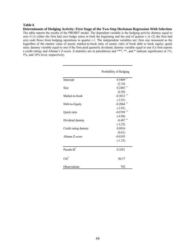
44
Table 6 Determinants of Hedging Activity: First Stage of the Two-Step Heckman Regression With Selection The table reports the results of the PROBIT model. The dependent variable is the hedging activity dummy equal to zero if (1) either the firm had zero hedge ratios in both the beginning and the end of quarter t; or (2) the firm had zero cash flows from hedging operations in quarter t-1. The independent variables are: firm size measured as the logarithm of the market value of assets; market-to-book ratio of assets; ratio of book debt to book equity; quick ratio; dummy variable equal to one if the firm paid quarterly dividend; dummy variable equal to one if a firm reports a credit rating; and Altman’s Z-score. Z-statistics are in parentheses and ***, **, and * indicate significance at 1%, 5%, and 10% level, respectively.
Intercept 0.5409 **
(2.10)Size 0.2403 ***
(4.50)Market-to-book -0.3013 ***
(-3.91)Debt-to-Equity -0.2064 ***
(-2.82)Quick ratio -0.0789 ***
(-4.98)Dividend dummy -0.487 ***
(-3.25)Credit rating dummy 0.0916
(0.61)Altman Z-score -0.0193
(-1.25)
Pseudo-R2 0.1051
Chi2 86.57
Observations 792
Probability of Hedging
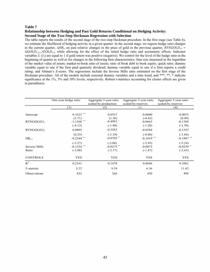
45
Table 7 Relationship between Hedging and Past Gold Returns Conditional on Hedging Activity: Second Stage of the Two-Step Heckman Regression with Selection The table reports the results of the second stage of the two-step Heckman procedure. In the first stage (see Table 6), we estimate the likelihood of hedging activity in a given quarter. In the second stage, we regress hedge ratio changes in the current quarter, ∆HRt, on past relative changes in the price of gold in the previous quarter, RTNGOLDt-1 = ∆GOLDt-2,t-1/GOLDt-2, while allowing for the effect of the initial hedge ratio and asymmetry effects. Indicator variables I1 (I2) are equal to 1 if gold return was positive (negative). We control for the level of the hedge ratio at the beginning of quarter as well as for changes in the following firm characteristics: firm size measured as the logarithm of the market value of assets; market-to-book ratio of assets; ratio of book debt to book equity; quick ratio; dummy variable equal to one if the firm paid quarterly dividend; dummy variable equal to one if a firm reports a credit rating; and Altman’s Z-score. The regressions include the Inverse Mills ratio estimated on the first stage of the Heckman procedure. All of the models include seasonal dummy variables and a time trend, and ***, **, * indicate significance at the 1%, 5% and 10% levels, respectively. Robust t-statistics accounting for cluster effects are given in parentheses.
Intercept 0.1623 *** 0.0337 -0.0040 0.0053(3.71) (1.36) (-0.42) (0.49)
RTNGOLD∙I1 -1.1368 *** -0.4991 * -0.0665 -0.1389(-4.13) (-1.80) (-1.20) (-1.50)
RTNGOLD∙I2 0.0805 -0.3583 -0.0584 -0.1552(0.25) (-1.59) (-0.80) (-1.04)
HRt-1 -0.2344 *** -0.0705 ** -0.1019 *** -0.1907 ***
(-3.27) (-2.06) (-2.95) (-5.24)Inverse Mills -0.1254 *** -0.0275 ** -0.0072 -0.0259 **
Ratio (-3.08) (-2.17) (-1.47) (-2.63)
CONTROLS YES YES YES YES
R2 0.2161 0.1478 0.0646 0.1061
F-statistic 5.22 9.39 6.36 11.62
Observations 432 366 430 495
(1) (2) (4)(3)scaled by production scaled by reservesscaled by reserves
One-year hedge ratio Aggregate 3-year ratio Aggregate 5-year ratioAggregate 3-year ratio
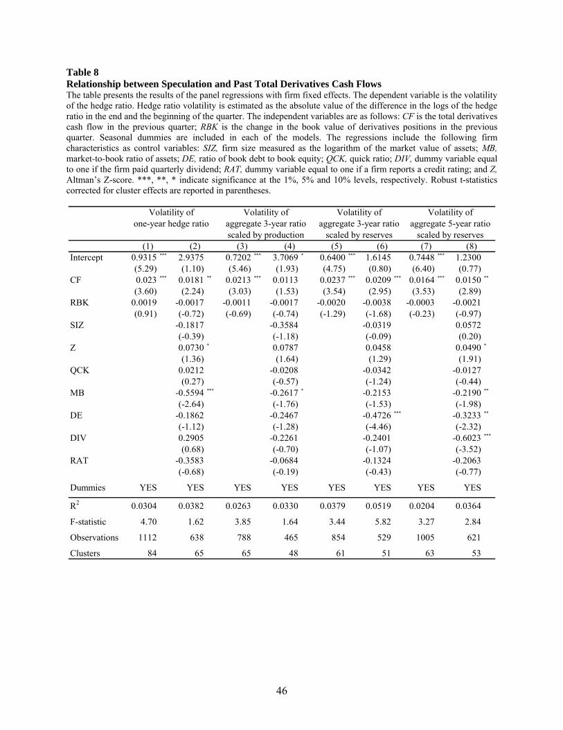
46
Table 8 Relationship between Speculation and Past Total Derivatives Cash Flows The table presents the results of the panel regressions with firm fixed effects. The dependent variable is the volatility of the hedge ratio. Hedge ratio volatility is estimated as the absolute value of the difference in the logs of the hedge ratio in the end and the beginning of the quarter. The independent variables are as follows: CF is the total derivatives cash flow in the previous quarter; RBK is the change in the book value of derivatives positions in the previous quarter. Seasonal dummies are included in each of the models. The regressions include the following firm characteristics as control variables: SIZ, firm size measured as the logarithm of the market value of assets; MB, market-to-book ratio of assets; DE, ratio of book debt to book equity; QCK, quick ratio; DIV, dummy variable equal to one if the firm paid quarterly dividend; RAT, dummy variable equal to one if a firm reports a credit rating; and Z, Altman’s Z-score. ***, **, * indicate significance at the 1%, 5% and 10% levels, respectively. Robust t-statistics corrected for cluster effects are reported in parentheses.
Intercept 0.9315 *** 2.9375 0.7202 *** 3.7069 * 0.6400 *** 1.6145 0.7448 *** 1.2300(5.29) (1.10) (5.46) (1.93) (4.75) (0.80) (6.40) (0.77)
CF 0.023 *** 0.0181 ** 0.0213 *** 0.0113 0.0237 *** 0.0209 *** 0.0164 *** 0.0150 **
(3.60) (2.24) (3.03) (1.53) (3.54) (2.95) (3.53) (2.89)RBK 0.0019 -0.0017 -0.0011 -0.0017 -0.0020 -0.0038 -0.0003 -0.0021
(0.91) (-0.72) (-0.69) (-0.74) (-1.29) (-1.68) (-0.23) (-0.97)SIZ -0.1817 -0.3584 -0.0319 0.0572
(-0.39) (-1.18) (-0.09) (0.20)Z 0.0730 * 0.0787 0.0458 0.0490 *
(1.36) (1.64) (1.29) (1.91)QCK 0.0212 -0.0208 -0.0342 -0.0127
(0.27) (-0.57) (-1.24) (-0.44)MB -0.5594 *** -0.2617 * -0.2153 -0.2190 **
(-2.64) (-1.76) (-1.53) (-1.98)DE -0.1862 -0.2467 -0.4726 *** -0.3233 **
(-1.12) (-1.28) (-4.46) (-2.32)DIV 0.2905 -0.2261 -0.2401 -0.6023 ***
(0.68) (-0.70) (-1.07) (-3.52)RAT -0.3583 -0.0684 -0.1324 -0.2063
(-0.68) (-0.19) (-0.43) (-0.77)
Dummies YES YES YES YES YES YES YES YES
R2 0.0304 0.0382 0.0263 0.0330 0.0379 0.0519 0.0204 0.0364
F-statistic 4.70 1.62 3.85 1.64 3.44 5.82 3.27 2.84
Observations 1112 638 788 465 854 529 1005 621
Clusters 84 65 65 48 61 51 63 53
Volatility of Volatility of Volatility of Volatility of
scaled by production scaled by reserves scaled by reserves(1) (2) (3) (4) (5) (6) (7) (8)
one-year hedge ratio aggregate 3-year ratio aggregate 3-year ratio aggregate 5-year ratio
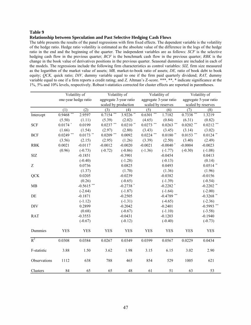
47
Table 9 Relationship between Speculation and Past Selective Hedging Cash Flows The table presents the results of the panel regressions with firm fixed effects. The dependent variable is the volatility of the hedge ratio. Hedge ratio volatility is estimated as the absolute value of the difference in the logs of the hedge ratio in the end and the beginning of the quarter. The independent variables are as follows: SCF is the selective hedging cash flow in the previous quarter; BCF is the benchmark cash flow in the previous quarter; RBK is the change in the book value of derivatives positions in the previous quarter. Seasonal dummies are included in each of the models. The regressions include the following firm characteristics as control variables: SIZ, firm size measured as the logarithm of the market value of assets; MB, market-to-book ratio of assets; DE, ratio of book debt to book equity; QCK, quick ratio; DIV, dummy variable equal to one if the firm paid quarterly dividend; RAT, dummy variable equal to one if a firm reports a credit rating; and Z, Altman’s Z-score. ***, **, * indicate significance at the 1%, 5% and 10% levels, respectively. Robust t-statistics corrected for cluster effects are reported in parentheses.
Intercept 0.9468 *** 2.9597 0.7154 *** 3.9226 ** 0.6301 *** 1.7182 0.7338 *** 1.3219(5.50) (1.11) (5.39) (2.02) (4.65) (0.84) (6.31) (0.82)
SCF 0.0174 * 0.0199 0.0237 *** 0.0210 ** 0.0273 *** 0.0263 *** 0.0202 *** 0.0212 ***
(1.66) (1.54) (2.97) (2.80) (3.43) (3.45) (3.14) (3.02)BCF 0.0249 *** 0.0173 ** 0.0209 *** 0.0092 0.0224 *** 0.0180 ** 0.0153 *** 0.0124 **
(3.56) (2.15) (2.95) (1.26) (3.39) (2.50) (3.40) (2.49)RBK 0.0021 -0.0117 -0.0012 -0.0020 -0.0021 -0.0040 * -0.0004 -0.0023
(0.96) (-0.73) (-0.72) (-0.86) (-1.36) (-1.77) (-0.30) (-1.08)SIZ -0.1851 -0.3901 -0.0454 0.0413
(-0.40) (-1.28) (-0.13) (0.14)Z 0.0736 0.0825 0.0493 0.0514 **
(1.37) (1.70) (1.36) (1.96)QCK 0.0205 -0.0239 -0.0382 -0.0156
(0.26) (-0.65) (-1.39) (-0.54)MB -0.5615 *** -0.2738 * -0.2282 * -0.2202 **
(-2.64) (-1.87) (-1.64) (-2.00)DE -0.1871 -0.2505 -0.4789 *** -0.3268 **
(-1.12) (-1.31) (-4.65) (-2.36)DIV 0.2899 -0.2042 -0.2401 -0.5993 ***
(0.68) (-0.67) (-1.10) (-3.58)RAT -0.3553 -0.0431 -0.1203 -0.1940
(-0.67) (-0.12) (-0.40) (-0.73)
Dummies YES YES YES YES YES YES YES YES
R2 0.0308 0.0384 0.0267 0.0349 0.0399 0.0567 0.0229 0.0434
F-statistic 3.88 1.50 3.62 1.98 3.15 6.15 3.02 2.90
Observations 1112 638 788 465 854 529 1005 621
Clusters 84 65 65 48 61 51 63 53
(5) (6) (7) (8)(1) (2) (3) (4)
Volatility of Volatility of Volatility of Volatility ofone-year hedge ratio aggregate 3-year ratio aggregate 3-year ratio aggregate 5-year ratio
scaled by production scaled by reserves scaled by reserves
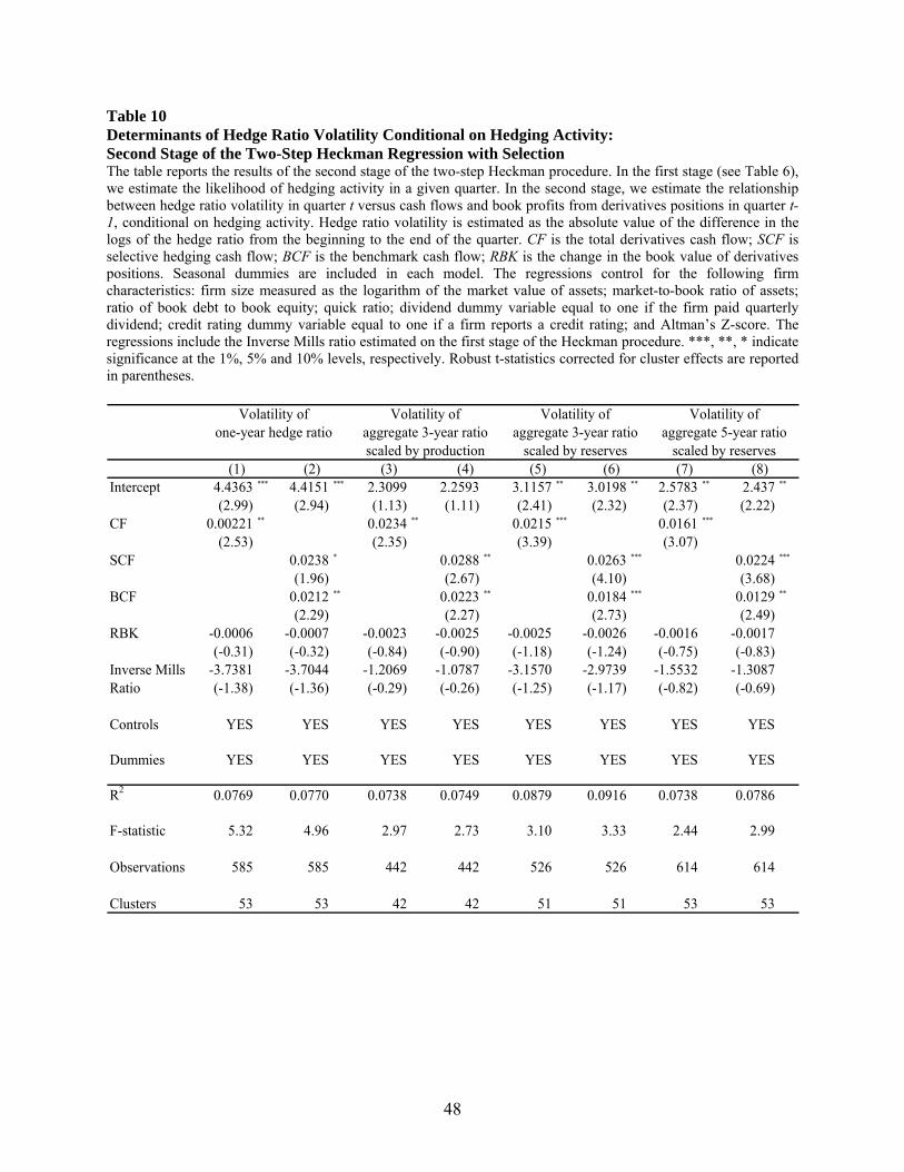
48
Table 10 Determinants of Hedge Ratio Volatility Conditional on Hedging Activity: Second Stage of the Two-Step Heckman Regression with Selection The table reports the results of the second stage of the two-step Heckman procedure. In the first stage (see Table 6), we estimate the likelihood of hedging activity in a given quarter. In the second stage, we estimate the relationship between hedge ratio volatility in quarter t versus cash flows and book profits from derivatives positions in quarter t-1, conditional on hedging activity. Hedge ratio volatility is estimated as the absolute value of the difference in the logs of the hedge ratio from the beginning to the end of the quarter. CF is the total derivatives cash flow; SCF is selective hedging cash flow; BCF is the benchmark cash flow; RBK is the change in the book value of derivatives positions. Seasonal dummies are included in each model. The regressions control for the following firm characteristics: firm size measured as the logarithm of the market value of assets; market-to-book ratio of assets; ratio of book debt to book equity; quick ratio; dividend dummy variable equal to one if the firm paid quarterly dividend; credit rating dummy variable equal to one if a firm reports a credit rating; and Altman’s Z-score. The regressions include the Inverse Mills ratio estimated on the first stage of the Heckman procedure. ***, **, * indicate significance at the 1%, 5% and 10% levels, respectively. Robust t-statistics corrected for cluster effects are reported in parentheses.
Intercept 4.4363 *** 4.4151 *** 2.3099 2.2593 3.1157 ** 3.0198 ** 2.5783 ** 2.437 **
(2.99) (2.94) (1.13) (1.11) (2.41) (2.32) (2.37) (2.22)CF 0.00221 ** 0.0234 ** 0.0215 *** 0.0161 ***
(2.53) (2.35) (3.39) (3.07)SCF 0.0238 * 0.0288 ** 0.0263 *** 0.0224 ***
(1.96) (2.67) (4.10) (3.68)BCF 0.0212 ** 0.0223 ** 0.0184 *** 0.0129 **
(2.29) (2.27) (2.73) (2.49)RBK -0.0006 -0.0007 -0.0023 -0.0025 -0.0025 -0.0026 -0.0016 -0.0017
(-0.31) (-0.32) (-0.84) (-0.90) (-1.18) (-1.24) (-0.75) (-0.83)Inverse Mills -3.7381 -3.7044 -1.2069 -1.0787 -3.1570 -2.9739 -1.5532 -1.3087Ratio (-1.38) (-1.36) (-0.29) (-0.26) (-1.25) (-1.17) (-0.82) (-0.69)
Controls YES YES YES YES YES YES YES YES
Dummies YES YES YES YES YES YES YES YES
R2 0.0769 0.0770 0.0738 0.0749 0.0879 0.0916 0.0738 0.0786
F-statistic 5.32 4.96 2.97 2.73 3.10 3.33 2.44 2.99
Observations 585 585 442 442 526 526 614 614
Clusters 53 53 42 42 51 51 53 53
(5) (6) (7) (8)(1) (2) (3) (4)
Volatility of Volatility of Volatility of Volatility ofone-year hedge ratio aggregate 3-year ratio aggregate 3-year ratio aggregate 5-year ratio
scaled by production scaled by reserves scaled by reserves

49
Table 11 Determinants of Hedge Ratio Volatility Conditional on Hedging Activity: Controlling for Managerial Compensation (CEO) The table reports the results of the second stage of the two-step Heckman procedure. In the first stage (see Table 6), we estimate the likelihood of hedging activity in a given quarter. In the second stage, we estimate the relationship between hedge ratio volatility in quarter t versus cash flows and book profits from derivatives positions in quarter t-1, conditional on hedging activity. Hedge ratio volatility is estimated as the absolute value of the difference in the logs of the hedge ratio from the beginning to the end of the quarter. CF is the total derivatives cash flow; SCF is selective hedging cash flow; BCF is the benchmark cash flow; DELTA_CEO and VEGA_CEO are the managerial compensation sensitivities for the CEO. The regressions include the Inverse Mills ratio estimated on the first stage of the Heckman procedure. ***, **, * indicate significance at the 1%, 5% and 10% levels, respectively. Robust t-statistics corrected for cluster effects are reported in parentheses.
Intercept 0.2460 0.2453 1.4696 1.4616 1.0222 1.0261 1.7445 1.7351(0.21) (0.21) (0.81) (0.81) (0.78) (0.78) (1.26) (1.24)
CF 0.0159 0.0183 0.0161 ** 0.0171 **
(1.35) (1.19) (2.08) (2.82)SCF 0.0143 0.0169 0.0182 ** 0.0212 **
(0.79) (0.81) (2.03) (2.74)BCF 0.0164 0.0186 0.0155 ** 0.0159 **
(1.47) (1.25) (2.05) (2.72)DELTA_CEO -0.1665 -0.1638 -0.1755 -0.1725 -0.1250 -0.1291 -0.1260 -0.1346
(-0.96) (-0.95) (-0.88) (-0.91) (-1.12) (-1.20) (-1.18) (-1.31)VEGA_CEO 0.2002 0.1963 0.0822 0.0788 0.0738 0.0791 0.0176 0.0291
(1.18) (1.18) (0.35) (0.35) (0.53) (0.58) (0.12) (0.19)
Inverse Mills 0.1638 3.1772 1.9141 1.9362 1.0782 1.0549 0.2416 0.2517Ratio (1.76) (1.75) (1.09) (1.11) (0.87) (0.86) (0.32) (0.34)
R2 0.0545 0.0544 0.037 0.0371 0.0407 0.0409 0.0466 0.0478
F-statistic 2.08 1.64 1.46 1.16 2.19 1.91 3.41 3.30
Observations 146 146 106 106 127 127 155 155
Clusters 41 41 31 31 39 39 42 42
Volatility of Volatility of Volatility of Volatility of
scaled by production scaled by reserves scaled by reservesone-year ratio aggregate 3-year ratio aggregate 3-year ratio aggregate 5-year ratio
(1) (2) (3) (4) (5) (6) (7) (8)
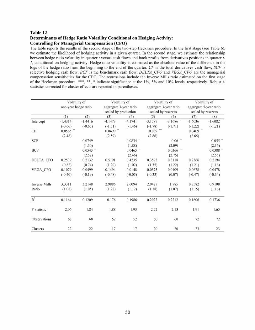
50
Table 12 Determinants of Hedge Ratio Volatility Conditional on Hedging Activity: Controlling for Managerial Compensation (CFO) The table reports the results of the second stage of the two-step Heckman procedure. In the first stage (see Table 6), we estimate the likelihood of hedging activity in a given quarter. In the second stage, we estimate the relationship between hedge ratio volatility in quarter t versus cash flows and book profits from derivatives positions in quarter t-1, conditional on hedging activity. Hedge ratio volatility is estimated as the absolute value of the difference in the logs of the hedge ratio from the beginning to the end of the quarter. CF is the total derivatives cash flow; SCF is selective hedging cash flow; BCF is the benchmark cash flow; DELTA_CFO and VEGA_CFO are the managerial compensation sensitivities for the CEO. The regressions include the Inverse Mills ratio estimated on the first stage of the Heckman procedure. ***, **, * indicate significance at the 1%, 5% and 10% levels, respectively. Robust t-statistics corrected for cluster effects are reported in parentheses.
Intercept -1.4314 -1.4416 -4.1473 -4.1741 -3.1787 -3.1686 * -1.6036 -1.6082(-0.66) (-0.65) (-1.51) (-1.46) (-1.78) (-1.71) (-1.22) (-1.21)
CF 0.0565 ** 0.0499 ** 0.039 *** 0.0409 **
(2.48) (2.59) (2.86) (2.65)SCF 0.0749 0.0834 * 0.06 ** 0.055 **
(1.50) (1.88) (2.09) (2.16)BCF 0.0543 ** 0.0465 ** 0.0366 *** 0.0388 **
(2.52) (2.46) (2.75) (2.55)DELTA_CFO 0.2539 0.2132 0.5191 0.4235 0.3593 0.3118 0.2366 0.2194
(0.82) (0.74) (1.20) (1.02) (1.35) (1.22) (1.21) (1.16)VEGA_CFO -0.1079 -0.0499 -0.1494 -0.0148 -0.0575 0.0109 -0.0678 -0.0478
(-0.40) (-0.19) (-0.48) (-0.05) (-0.33) (0.07) (-0.47) (-0.34)
Inverse Mills 3.3311 3.2148 2.9886 2.6094 2.0427 1.785 0.7582 0.9108Ratio (1.08) (1.05) (1.22) (1.12) (1.18) (1.07) (1.15) (1.16)
R2 0.1164 0.1209 0.176 0.1986 0.2023 0.2212 0.1606 0.1736
F-statistic 2.06 1.84 1.88 1.93 2.22 2.13 1.91 1.65
Observations 68 68 52 52 60 60 72 72
Clusters 22 22 17 17 20 20 23 23
(5) (6) (7) (8)(1) (2) (3) (4)scaled by production scaled by reserves scaled by reserves
one-year hedge ratio aggregate 3-year ratio aggregate 3-year ratio aggregate 5-year ratioVolatility of Volatility of Volatility of Volatility of
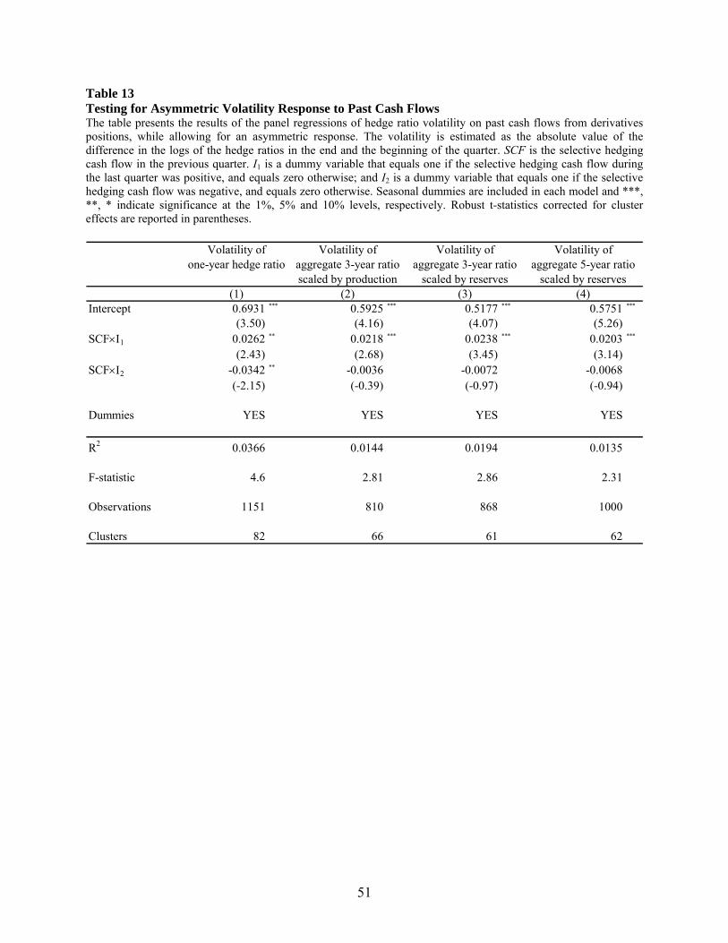
51
Table 13 Testing for Asymmetric Volatility Response to Past Cash Flows The table presents the results of the panel regressions of hedge ratio volatility on past cash flows from derivatives positions, while allowing for an asymmetric response. The volatility is estimated as the absolute value of the difference in the logs of the hedge ratios in the end and the beginning of the quarter. SCF is the selective hedging cash flow in the previous quarter. I1 is a dummy variable that equals one if the selective hedging cash flow during the last quarter was positive, and equals zero otherwise; and I2 is a dummy variable that equals one if the selective hedging cash flow was negative, and equals zero otherwise. Seasonal dummies are included in each model and ***, **, * indicate significance at the 1%, 5% and 10% levels, respectively. Robust t-statistics corrected for cluster effects are reported in parentheses.
Intercept 0.6931 *** 0.5925 *** 0.5177 *** 0.5751 ***
(3.50) (4.16) (4.07) (5.26)SCF×Ι1 0.0262 ** 0.0218 *** 0.0238 *** 0.0203 ***
(2.43) (2.68) (3.45) (3.14)SCF×Ι2 -0.0342 ** -0.0036 -0.0072 -0.0068
(-2.15) (-0.39) (-0.97) (-0.94)
Dummies YES YES YES YES
R2 0.0366 0.0144 0.0194 0.0135
F-statistic 4.6 2.81 2.86 2.31
Observations 1151 810 868 1000
Clusters 82 66 61 62
Volatility of Volatility of Volatility of Volatility of
scaled by production scaled by reserves scaled by reservesone-year hedge ratio aggregate 3-year ratio aggregate 3-year ratio aggregate 5-year ratio
(1) (2) (3) (4)
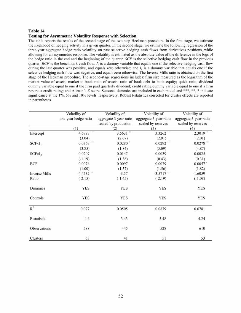
52
Table 14 Testing for Asymmetric Volatility Response with Selection The table reports the results of the second stage of the two-step Heckman procedure. In the first stage, we estimate the likelihood of hedging activity in a given quarter. In the second stage, we estimate the following regression of the three-year aggregate hedge ratio volatility on past selective hedging cash flows from derivatives positions, while allowing for an asymmetric response. The volatility is estimated as the absolute value of the difference in the logs of the hedge ratio in the end and the beginning of the quarter. SCF is the selective hedging cash flow in the previous quarter. BCF is the benchmark cash flow. I1 is a dummy variable that equals one if the selective hedging cash flow during the last quarter was positive, and equals zero otherwise; and I2 is a dummy variable that equals one if the selective hedging cash flow was negative, and equals zero otherwise. The Inverse Mills ratio is obtained on the first stage of the Heckman procedure. The second-stage regressions includes: firm size measured as the logarithm of the market value of assets; market-to-book ratio of assets; ratio of book debt to book equity; quick ratio; dividend dummy variable equal to one if the firm paid quarterly dividend; credit rating dummy variable equal to one if a firm reports a credit rating; and Altman’s Z-score. Seasonal dummies are included in each model and ***, **, * indicate significance at the 1%, 5% and 10% levels, respectively. Robust t-statistics corrected for cluster effects are reported in parentheses.
Intercept 4.6787 *** 3.5631 ** 3.3262 *** 2.3019 **
(3.04) (2.07) (2.91) (2.01)SCF×Ι1 0.0369 *** 0.0280 * 0.0292 *** 0.0278 ***
(3.85) (1.84) (5.09) (4.87)SCF×Ι2 -0.0207 0.0147 0.0039 0.0025
(-1.19) (1.38) (0.43) (0.31)BCF 0.0076 0.0097 0.0079 0.0057 *
(1.00) (1.57) (1.56) (1.82)Inverse Mills -4.4532 ** -3.57 -3.5717 ** -1.6059Ratio (-2.15) (-1.45) (-2.19) (-1.08)
Dummies YES YES YES YES
Controls YES YES YES YES
R2 0.077 0.0505 0.0879 0.0781
F-statistic 4.6 3.43 5.48 4.24
Observations 588 445 528 610
Clusters 53 41 51 53
scaled by production scaled by reserves scaled by reservesone-year hedge ratio aggregate 3-year ratio aggregate 3-year ratio aggregate 5-year ratio
Volatility of Volatility of Volatility of Volatility of
(1) (2) (3) (4)