managerial economics prof. trupti mishra s.j.m …textofvideo.nptel.ac.in/110101005/lec22.pdf ·...
TRANSCRIPT

Managerial Economics
Prof. Trupti Mishra
S.J.M School of Management
Indian Institute of Technology, Bombay
Lecture - 22
Theory of Cost (Contd..)
So, in this session, we will continue our discussion on relationship between the total cost
total revenue profit and loss. The break even analysis what we discussed in the last
session also; and we will see, what is the profitable and non-profitable range of output,
how the business activities planned on the basis of profit and loss.
(Refer Slide Time: 00:42)
So, if you remember in the last class we talk about the long run cost and output
relationship. Generally, how the long run cost is derived from the short run cost curves
and how both of them they are related, in which case short run cost curve is use, and in
which case the long run cost curve is used. Then, we introduce the break even analysis to
specifically in case of linear cost and revenue function, when linear cost and revenue
follow a straight line. So, the breakeven point is one where the total cost is equal to total
revenue. Beyond that it is a profitable range of output, because total revenue is more than
total cost and before this it is a non-profitable range, because the total cost is greater than
the total revenue and the breakeven point is one, where the total cost is equal to total
revenue.

(Refer Slide Time: 01:34)
So, we will to start with we will continue again our discussion on the linear cost
function. We will just look at the algebra behind the linear cost and revenue function,
specifically in case of breakeven analysis. Then, we will discuss about the non-linear
cost and revenue function. Then, we will do the contribution analysis and then finally,
we will discuss about the learning curve, which is the again with the background is on
the shape of the long run average cost curve.
Generally, the practice is that we follow that there is economics of scale because of
which the average cost is decreasing, but learning curve is the alternate method to
understand or the expand that why the long run average cost is decreasing.

(Refer Slide Time: 02:19)
So, to start with we look at what is the algebra behind the breakeven analysis. So,
actually, we know that at the breakeven point the total revenue equal to total cost. So,
actually know total revenue is team multiplied by Q and total cost has two parts; that is,
total fixed cost and total variable cost. Now, this total variable cost is alternatively, we
can say this is the average variable cost multiplied by the quantity and total cost is total
fixed cost. And instead of TVC, if you write average variable cost multiplied by Q, then
this is this comes as total fixed cost and in place of total variable cost, we use average
variable cost multiplied by Q.
In this case, we can write this as the Q B is the breakeven level of output. If it is a
breakeven level of output, putting this total revenue is equal to total cost. Total revenue
is you teach PQ. So, QB by p and total cost is total fixed cost plus average variable cost.
And in case of this Q since QB is the breakeven level of output we will use QB.
So, QB by p multiplied by P is now simplify this again, this is ABC QB equal to total
fixed cost. Again simplifying this, we will get, if you take QB is out that is P-ABC,
which is equal to total fixed cost or we can say QB equal to total fixed cost divided by P-
ABC. So, if you in know or if the producer know what is the level of TFC. What is the
level of TBC and what is the level of p then, we can find out the quantity that is the
breakeven level of quantity through this that is QB equal to TFC by P-ABC.

So, the algebra behind this is, if you know the fixed cost and if you know the average
variable cost and if you know the price of it, generally, you can find out the find out the
breakeven level of output, but when it comes to break even analysis.
(Refer Slide Time: 05:15)
Specifically, in case of linear cost and revenue function, it is applicable only if the cost
and revenue are linear. So, in case of linear cost and revenue function the total cost and
total revenue are straight line they intersect only at one point dividing the whole range of
output plus two parts that is profitable and non profitable like in the previous.
(Refer Slide Time: 05:41)

So, that this is our total fixed cost, this is total variable cost, this is total revenue cost and
the total costs starts from here, and this is the total revenue cost, total cost this is the
breakeven level of output because total revenue is equal to total cost. And this divides
the entire range of output in to two level; that is non profitable and profitable. This is
possible only if it is a linear total revenue function. Linear total cost function because
they intersect each other only at one point and that is the reason clearly we can divide
that this is the profitable range of output and this is the non profitable range of output.
But if it is not a case of linear then the possibility is that they intersect more than twice or
may be more than once and in this case, it is difficult to find out what is the profitable
range of output and what is the non profitable range of output. So, what is the
implication for this? If it is a linear cost and revenue function, we get two range of
output; profitable range of output and non profitable range of output.
(Refer Slide Time: 07:03)
But, the implication for this that the whole output beyond the breakeven level is
profitable right because the point behind which the total revenue is equal to total cost.
The total revenue is more than the total cost beyond all the level which implies from the
linear cost and revenue function, but when it comes to the real life this is not the fact as
the conditions are different due to changing price and cost. So, it not possible that the
you get a when it say it is a case of linear cost and revenue function.

So, if you look at the graph beyond this point, we say any level of output is profitable
right. So, implication of linear cost and revenue function is that beyond the breakeven
level any level of output is profitable. But in the real life the fact is, condition is different
due to the changing price and cost and that leads to the fact that the cost of the revenue
and function may not be linear they may non-linear.
The cost function and the revenue function is non-linear because of the fact that the
incase of real life, there is a changing price which leads to change in the cost changing
price of inputs and changing price of raw materials, which leads to the variation in the
cost and which leads to the possibility that the cost and revenue of a non-linear.
(Refer Slide Time: 08:34)
So, the non-linearity arises because of average variable cost and the price vary with the
variation in the output, since the average variable cost changes due to change in the price
which vary with the variation in the output. And as a result total cost may increase at the
increasing rate and total revenue increase at the decreasing rate.
Since, there is a non-linearity because of average variable cost and price change with the
variation in the output. That leads to the possibility that total cost increase at the
increasing rate and total revenue increase at the decreasing rate. So, the stump stages of
output total cost exceeds the total revenue, but in case of linear cost how it was
happening. It was like after the break even level, the total revenue is always greater than
the total cost, but in case of non-linear since total level will increase at the decreasing

rate and total cost will increase at the increasing rate. At least at some stage of output the
possibility is that the total cost will increase the total revenue.
(Refer Slide Time: 09:47)
So, in this case may be we get two breakeven point. That is the one breakeven point
when total cost is equal to total revenue and the possibility is that the other breakeven
point is again. The total cost is that the total revenue which limits the profitable range of
output and determine the lower and upper limit of output.
So, it is not the profitable range of output is unlimited rather, it is the its define the lower
and upper limit of the profitable range of output. So, there is a need to pretest there is a
need to verify the validity of the linearity of cost and revenue function before assuming
that the cost of the revenue is the linear.
So, in this case there is a need of pretest. There is a need of verification before taking the
cost and revenue as the linear function. So, what happens in case of non-linear. There is
two break even points. There is not only one breakeven point, two breakeven point and
that decides the limit upper limit and lower limit of the ranges of the output.

(Refer Slide Time: 10:55)
So, let us find out the graph for the non-linear cost and revenue function. In case of a
break even analysis, this is total cost and revenue, this is output suppose, this is total
fixed cost this is total revenue.
(Refer Slide Time: 11:04)
So, this is total cost this is total revenue and this is total fixed cost. So, here the total
fixed cost line, it shows that the fixed cost that of this is fixed cost and the vertical
distance between total cost and total fixed cost. It measures the total variable cost
because this is the total fixed cost and total cost, which always the summation of the total

variable cost and total fixed cost. So, the vertical distance between the total cost and total
fixed cost that gives us the total variable cost.
The curve total revenue shows that the total sales or total revenue of different output
level at the different price and the vertical distance between the total revenue. Total cost
measures the profit or loss of variable level of output. So, the vertical distance between
total revenue and total cost that will give you the various level of output.
So, corresponding to that we get two various level of output one is Q1 second one is Q 2.
So, we can say this is P 1 and this is P 2. So, total revenue and cost intersect to each
other at two different point one at the point P1 second at the point P 2 where the total
revenue is equal to total cost.
Before the level P 1, the total cost is greater than total revenue. So, this is the non
profitable range of output beyond P 1 any level of output up to P 2. This is the profitable
range of output, but like in case of linear cost and revenue function, it is not unlimited.
The profitable range of output is unlimited because we get another breakeven point at P 2
which leads to the fact at beyond this point total cost is greater than total revenue and
again this range is non profitable range.
So, in case of non-linear cost function, we get two breakeven level and which also
identify the lower limit and upper limit of profitable range of output. So, Q 1 is the
beginning of the profitable range of output and Q 2 is the end of the profitable range of
output. This is the lower limit of profitable level of lower range of output where the
profit can be achieved. This is the higher level of output where the profit can be output.
So, this represents lower and upper breakeven point.
P1 is the lower breakeven point P 2 is the upper breakeven point and for the whole range
of output between oq1 and corresponding to the this and this q1 and q2 is the breakeven
point correspondent to this output level. The total revenue is greater than total cost. So,
this is the profit this is the lower breakeven point this is the upper breakeven point.
So, if the farm is producing more than OQ1 then or less than OQ 2, they are making the
profit. So, if the farm is producing more than oq1 it should be more than oq1 the Q
should be more than OQ 1and less than OQ2 then only the farm is making the profit. So,
the output level should be more than OQ 1 and less than OQ 2.
(Refer Slide Time: 15:37)
Generally, the farm is making the profit and producing less or more than the age limits
gives rites to the losses. So, basically the essential difference between the linear and non-
linear break even analysis is, incase of linear break even analysis is profitable range of
output is unlimited, but in case of non-linear analysis there is a limit of profitable range
of output.
Beyond that producing more before that producing less will lead to the loss. So, if you
look to that this is the loss because total cost is greater than total revenue. This is also
loss because the total cost is greater than total revenue. This is the profitable range of
output where the total revenue is greater than total cost. Then, we will come to the one
more type of analysis may be in relation to this break even analysis that is called as the
contribution analysis.

(Refer Slide Time: 16:39)
So, till the time here we are considering the total revenue total cost to understand the
break even analysis, but in case of a contribution analysis we are not taking the total cost
total revenue. We are taking the incremental revenue and incremental cost of the
business activity. So, contribution analysis is the analysis of incremental revenue and
incremental cost of business activity.
And break even charts can also be used to measuring the contribution made by business
activity towards covering the fixed cost. So, through contribution analysis will use some
break even charts and the what is the role of break even charts? Here the role of break
even charts over here is to measure the contribution made by the business activity
towards the covering the fixed cost and in the graph always the variable cost is flutted
below the fixed cost.

(Refer Slide Time: 17:34)
So, fixed cost are cost and (( )) to the variable cost. Total cost line will run parallel to the
variable cost line. The change in the total cost is depend on the change in the total
variable cost and the contribution is the difference between the total revenue and variable
cost arising out of the business decision. So, there will the difference between the total
revenue and total cost keeps us the profit and contribution which is strictly defined as
difference between the total revenue and the total variable cost.
(Refer Slide Time: 18:12)
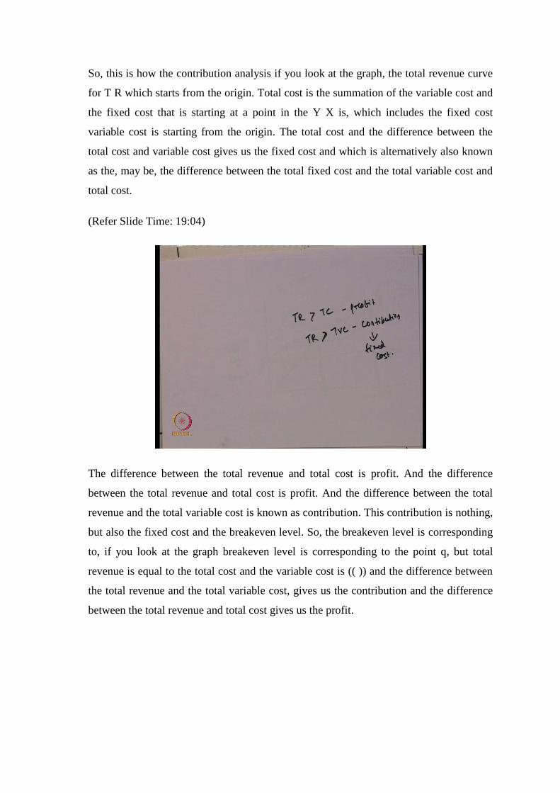
So, this is how the contribution analysis if you look at the graph, the total revenue curve
for T R which starts from the origin. Total cost is the summation of the variable cost and
the fixed cost that is starting at a point in the Y X is, which includes the fixed cost
variable cost is starting from the origin. The total cost and the difference between the
total cost and variable cost gives us the fixed cost and which is alternatively also known
as the, may be, the difference between the total fixed cost and the total variable cost and
total cost.
(Refer Slide Time: 19:04)
The difference between the total revenue and total cost is profit. And the difference
between the total revenue and total cost is profit. And the difference between the total
revenue and the total variable cost is known as contribution. This contribution is nothing,
but also the fixed cost and the breakeven level. So, the breakeven level is corresponding
to, if you look at the graph breakeven level is corresponding to the point q, but total
revenue is equal to the total cost and the variable cost is (( )) and the difference between
the total revenue and the total variable cost, gives us the contribution and the difference
between the total revenue and total cost gives us the profit.

(Refer Slide Time: 19:54)
So, if you look at this graph previously O Q is the breakeven level of output and the
contribution equals to the fixed cost below the output O Q to the total contribution is less
than the fixed cost. That is amount of loss below this the contribution is less than fixed
cost. That is the reason this is the amount of the loss and beyond this point the
contribution is more than the fixed cost. And that is the reason if you look at this the case
of the profit that is the contribution exceeds fixed cost. And the difference is the
contribution towards the profit resulting from the business decision. So, beyond the
before the breakeven level of output total contribution is less than fixed cost. So, this is
the amount to loss and beyond the output O Q that is beyond the breakeven level of
output contribution exceed the fixed cost and this is the difference in the contribution
towards the profit resulting from the business decision.
So, one is before breakeven level of output. The contribution is less than fixed cost. That
is the reason this leads to loss and the other point is beyond the breakeven level of output
which exceeds the fixed cost. The contribution exceeds the fixed cost and this is the
difference in the contribution towards the profit resulting from the business decision.

(Refer Slide Time: 21:32)
But, if you look at the contribution overtime period under the review is plotted in order
to indicate to the commitment that the management has made to fixed the expenditure.
Because there is a commitment, even the output leads to profitable output and not still
they have to incur a certain amount of the expenditure. And to find the level of output
from which it will be recover and profit will begin to immerge back will look from the
contribution.
(Refer Slide Time: 22:16)

So, if you look at the graph here. So, will just draw a graph that how the contribution
immerge when there is a commitment. When the management decides to or management
has the commitment to made to the fixed expenditure and there we need to find the level
of output from which level of output the fixed cost whatever, the contributed before that
can we recover and the new level of profit can be generated.
So, we will take a total revenue curve here as a straight line. This is the fixed cost to
make it simplify, we are not adding the variable cost. Here this is fixed cost and
contribution on the Y axis and output and the x axis. So, this is Q and this is the
contribution, but beyond the breakeven level since Q is the breakeven level of output
breakeven level of output OQ is the breakeven level of output. This is the loss because
the contribution is less than the fixed cost and at the point o Q the fixed cost is equal to
the contribution. And beyond this the fixed cost is less than the less than the contribution
that is why this is the net profit added to the firm beyond the breakeven level of output.
So, the output level of O Q contribution equals to fixed cost before this the contribution
is less than the fixed cost. That is why the firm is incurring loss and beyond this point the
contribution is more than the fixed cost and that is the reason the firm is getting the
profit.
(Refer Slide Time: 24:39)
Next, we look at the profit volume ratio. So, profit volume ratio is another useful tool for
finding the breakeven point for sales, especially, for the multipurpose firm. So, this is the

breakeven point in the short firm is known as B E P. that is, of sales especially for the
multipurpose firm and what is the P V ratio P V ratio is s – b 100 whereas, s is the selling
price b is the average variable cost. So, the profit volume ratio is the difference between
the selling price and the average variable cost and this is P V ratio is generally use as the
breakeven point for the sales particular in the multipurpose firm.
(Refer Slide Time: 25:19)
So, if you the selling price is the s is equal to 5 unit the average variable cost is b is equal
to the rupees 4 unit then P V ratio is selling price that is 5 minus variable cost 4 open 5
multiplied by 100 that is 20 percent we can say that 20 percent is the p v volume ratio.
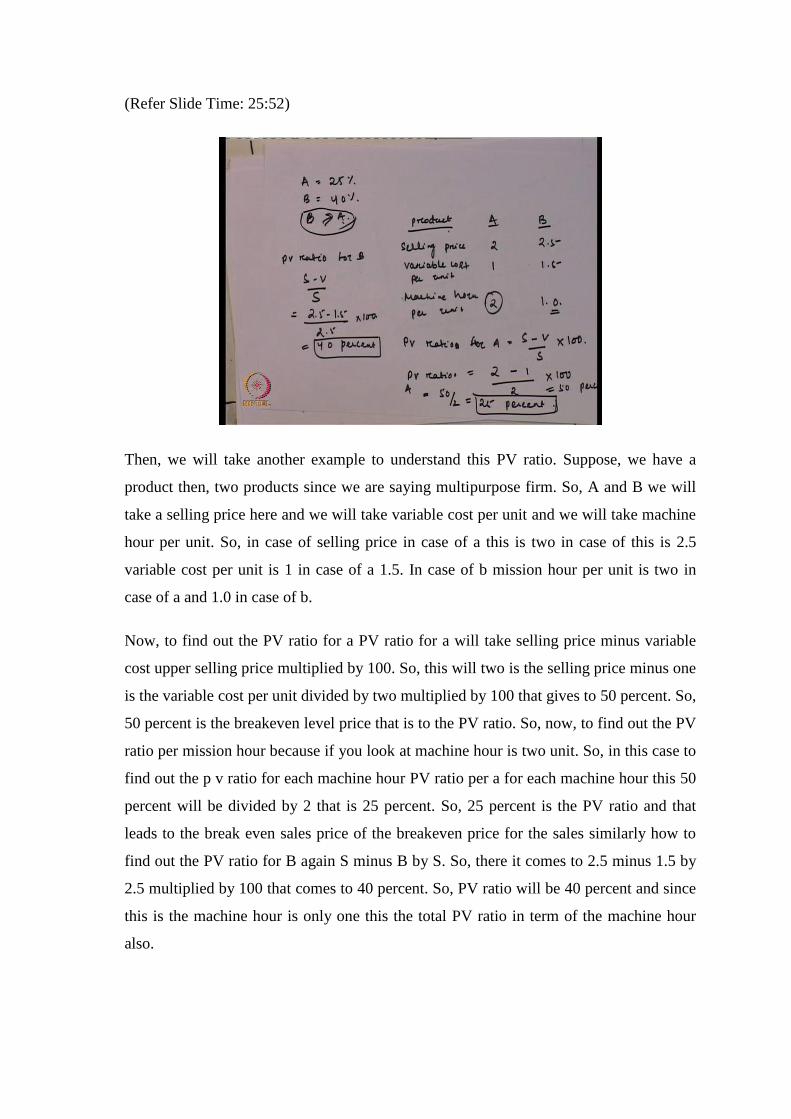
(Refer Slide Time: 25:52)
Then, we will take another example to understand this PV ratio. Suppose, we have a
product then, two products since we are saying multipurpose firm. So, A and B we will
take a selling price here and we will take variable cost per unit and we will take machine
hour per unit. So, in case of selling price in case of a this is two in case of this is 2.5
variable cost per unit is 1 in case of a 1.5. In case of b mission hour per unit is two in
case of a and 1.0 in case of b.
Now, to find out the PV ratio for a PV ratio for a will take selling price minus variable
cost upper selling price multiplied by 100. So, this will two is the selling price minus one
is the variable cost per unit divided by two multiplied by 100 that gives to 50 percent. So,
50 percent is the breakeven level price that is to the PV ratio. So, now, to find out the PV
ratio per mission hour because if you look at machine hour is two unit. So, in this case to
find out the p v ratio for each machine hour PV ratio per a for each machine hour this 50
percent will be divided by 2 that is 25 percent. So, 25 percent is the PV ratio and that
leads to the break even sales price of the breakeven price for the sales similarly how to
find out the PV ratio for B again S minus B by S. So, there it comes to 2.5 minus 1.5 by
2.5 multiplied by 100 that comes to 40 percent. So, PV ratio will be 40 percent and since
this is the machine hour is only one this the total PV ratio in term of the machine hour
also.

In case of a the P V ratio is 25 percent. In case of B the PV ratio is 40 percent. So, in this
case B and P preferable to a or the in the other word, we can say the firm will get more
breakeven or more get profit from b is compared to the a because the PV ratio is more in
case of b compared to a and PV ratio is nothing, but the difference between the selling
price and the selling price and the variable cost of production. So, the larger is the larger
is the variation more profit to the firm because that finally, lead to the breakeven price
for the sales for the typical product.
(Refer Slide Time: 29:33)
Then, we will discuss about the. So, the breakeven point in the sales men which
calculated by dividing the fixed expenses saved by the PV ratio. So, BEP sales value is
the fixed expenses by PV ratio which is equal to A by S minus P divided by S.

(Refer Slide Time: 29:50)
Then, we will talk about the margin of sep t and margin of sep t generally represents the
difference between sales and breakeven point and total actual cost. So, the difference
between the sales and the breakeven point and the total actual cost will leads to the
margin of sep t. There are three majors to this margin of sept; one that is profit multiplied
by sales by PV ratio second profit by PV ratio and third margin of sep T is SM minus SB
divided by S m multiplied by 100 where S a is the actual sales S b is the sales at the b p.
(Refer Slide Time: 30:35)

So, we will just take a example to understand this margin of sep T. So, here total revenue
is 10 Q total cost is 50 plus 5 Q and s is 20. So, given the total revenue and total cost
from sales and B P S B can be if you look at. So, total revenue is ten s b and total cost is
50 plus 5 S b because this is a sales at the breakeven level of output which is equal to q
then at the breakeven point is equal to total cost. So, substituting the value of total
revenue and total cost that is ten s b is equal to 50 plus 5 S b. So, 10 S b minus 5 S b
which is equal to 50. So, 5 S b is equal to 50 and S b is equal to 10.
Now, in order to find the margin of sep t we know that s b is equal to ten and s c is equal
to twenty. So, following the third major that is s a minus s b by s a multiplied by hundred
will give us the margin of sept here s a is the actual sales this is the breakeven sales. So,
corresponding to this we will get marginal of sep t is equal to 20 minus 10 that is 20
multiplied by 100 which is equal to 50 percent. So, this margin of sep t can be increased
by increasing the selling price provided that demand of product is inelastic. Because if it
is elastic then small change in the price is going to get influence by the consumer and
they will change the demand pattern.
So, the margin of sep t is the difference between the actual sales and the break even
sales. And break even sales and can be find out from total cost and total revenue. So,
margin of sep t in the last class will look at the more is the actual sale that is s a that
more is the margin of sep t.
(Refer Slide Time: 33:28)
So, it can be increased by increasing the selling price. The sales can be increased by
increasing the selling price probed, the sales are not seriously affected and it can happen
only when the demand for product is inelastic. Because if it is elastic, whenever there is
change in the change in the price selling price that leads to effect the demand in one way.
That will reduce the sales the quantity of the sales also this margin of sep T can be
increased by increasing the production. And sales up to the capacity of the plan even by
reducing the selling price provided the demand is elastic.
So, it can be also increased by increasing the production and sales up to the capacity of
plan even by reducing the selling price and here again the precondition is the demand is
elastic.
(Refer Slide Time: 34:22)
So, this for a margin of sept, the other method includes the reduction in the fixed
caption's in order to increase the margin of sep t. The other methods to increase the
margin of sep t is to reduction in the fixed expenses. Reduction in the variable expenses
or having a product mix with the greater share of one that assure a greater contribution
per unit which has a higher p v ratio the profit volume ratio.
So, either the margin of sep T can be increased by reducing the fixed expenses. Reducing
the variable expenses or using the product is which keeps more contribution. That is
more than the fixed cost and also a higher p v ratio the profit volume ratio. So, margin of

sep t will be increased by reducing the expenses; both fixed expenses and the variable
expenses or get it share of contribution of the greatest value of the p v ratio.
(Refer Slide Time: 35:25)
So, when it comes to this break even analysis, whether it is a contribution analysis
through the p v ratio or through any other method, if you look it can only be applied to
the single product system or can it be applied when the cost and price data cannot be
determined beforehand. So, there is a limitation to the break even analysis. If its
applicable only to the single product system and it can be applied only if the cost and
price data is known before hand.

Refer Slide Time: 35:56)
Then, we will talk about the concept of learning curve and if you look at we are going on
discussing one fact across this session that this long run average cost curve is use.
(Refer Slide Time: 36:04)
If and this use if is decreasing part because of economy of scale the reduce cost is
because of economy of scale and the increasing part is because of diseconomic of scale.
But, if you look at there may be other reason through almost must be understand that this
reduced cost it not only because of economic of scale or the increase cost is not because
of diseconomic of scale. There may be few other factors which influence the increasing

and decreasing average cost of production when there is the scale of output increases. So,
one of the fact here is that per knowledge and experience farm reducing the long run
average cost curve most continuously they learn about time to get work done about
shorter period of time reduce cost of production and increase cost of time is the fact of
productivity.
Like, if you take the case of labour, if you take the case of capital I think when you the
opinion of the farmer. The opinion of the learning prominent of learning is that, when the
firm does the same type of production over a period of time they get experience in doing
that and that leads to less time that leads to less cost of production and increase the factor
or productivity. So, the efficiency of the inputs increases the efficiency of the firm
increases and that is the reason the cost is decreasing. So, the learning cost the theory we
had learning cost is, that it’s not because of economic age of scale or the dis economic
age of scale. There is one more fact that the knowledge and experiencing in doing the
same kind of activity, they learn through and that leads to the average cost decreases.
Suppose, some are new to operate that machine and if the labour is operating that
machine over a period of time, he gain the scale again. He gains the exposure to operate
this operate the machine and he is doing the whatever time is requiring time request to
operate the machine. That is come down and may be also the productivity of the labour
increase because in the same time he can do something else.
Now, similarly if you look at the process itself, the process itself the initially there is a
time to fix up or set up the process. But in the long run when you do it over a period of
time, the process is set up the system is in place and that leads to less time and the inputs
become more productive.
So, in case of learning curve the opinion is that the one knowledge and experience help
the firms to reduce the average cost. And that leads to the shorter period of time reduce
cost to the production and increase the factor productivity.

(Refer Slide Time: 38:51)
And this learning curve is one that is applicable to the accumulative output and it’s not
the output. May be, average output the major difference between the long run average
cost curve and the learning curve is in case of long run average cost curve. We take the
average cost of production with the increase in the scale of output. But in case of
learning curve we take the accumulative of output that is the total product from the
beginning of the stage.
(Refer Slide Time: 39:30)

So, if you look at this curve is showing a decline trained in the. So, if this is the learning
curve its decreasing, but in case of long run average cost curve it always increases after a
point. But in case of learning curve in case of learning curve it the accumility cost
cumility of output in case of average cost goes on decreasing there is no shine to increase
the cost of production when the scale of output increases.
(Refer Slide Time: 40:08)
So, this curve shows the declining trained in long term average cost of production and
learning curve is different from the conventional long run. Average cost curve as long
run average cost curve gives the cost of plan wise production learning curve gives the
average cost of accumility of output.

(Refer Slide Time: 40:41)
The total output right from the beginning of the production from the accomodity. Now,
we will say we will take a small numerical to understand this learning curve or we will
do the or will estimate the unit of the learning curve. So, if you take a cost function
where c is equal to a Q to the power b where, c is the average cost and Q is the average
cost of unit of output Q. A is the cost unit of output and b is the rate of decreasing rate of
decreasing average cost with cumility of increasing output. The value of b is negative
because decrease in Q will always increase the or may be decrease in the cost with
cumility will increase in the output the greater the value of b the first one is the decrease
in the average cost.
(Refer Slide Time: 42:21)
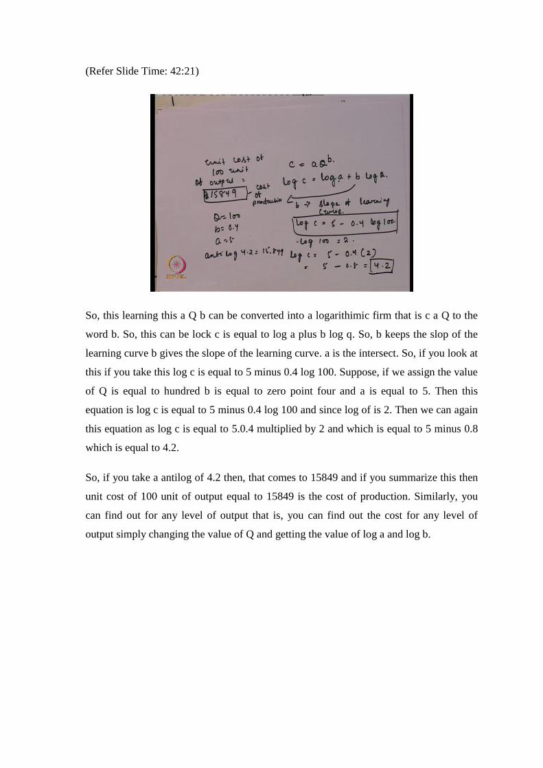
So, this learning this a Q b can be converted into a logarithimic firm that is c a Q to the
word b. So, this can be lock c is equal to log a plus b log q. So, b keeps the slop of the
learning curve b gives the slope of the learning curve. a is the intersect. So, if you look at
this if you take this log c is equal to 5 minus 0.4 log 100. Suppose, if we assign the value
of Q is equal to hundred b is equal to zero point four and a is equal to 5. Then this
equation is log c is equal to 5 minus 0.4 log 100 and since log of is 2. Then we can again
this equation as log c is equal to 5.0.4 multiplied by 2 and which is equal to 5 minus 0.8
which is equal to 4.2.
So, if you take a antilog of 4.2 then, that comes to 15849 and if you summarize this then
unit cost of 100 unit of output equal to 15849 is the cost of production. Similarly, you
can find out for any level of output that is, you can find out the cost for any level of
output simply changing the value of Q and getting the value of log a and log b.

(Refer Slide Time: 44:43)
So, if you summarize whatever we discussed today, taking this break even analysis
learning curve and p v ratio. The business manager must plan for the long run addition of
the cost revenue and profit and because in the long run firm in the position to expand the
scale of production by increasing all inputs. So, the it is a kind of scenario analysis. It’s a
kind of long term horizon how the firm because the firms decision firms business
decision firms depends upon the cost and revenue because that gives us the profitable
and non profitable range of output.
(Refer Slide Time: 45:19)

So, in the long run with the increase in output, the total cost of production first increases
at the decreasing rate then at an increasing rate and as a (( )) long run as the average cost
initially decreases until the optimum utilization of new plan (( )) and then it began to
increase. And the cost and the output relation always follow a loss of return to scale and
that is the reason the long run average cost for which show a usage. So, the decreasing
part of the long run average cost per decrease the economic scale and long run increasing
part is because of diseconomic of scale.
(Refer Slide Time: 45:55)
Firms are assume to plan the production activity much better level of production for
which total cost and total revenue break even is known and this employees the profitable
and non profitable range of output.
(Refer Slide Time: 46:04)
So, we analyse the break-even analysis for both linear and the non-linear total cost and
revenue analysis. So, the break-even analysis or the profit contribution analysis is the
analytical technique used in studying the relationship between the total cost total revenue
total profit and losses over a range of stipulated output. And basically there is a
technique of previewing the profit prospect and tool of planning.
So, if you remember in case of linear cost and revenue, we get one breakeven level of
output where the profitable range of output is unlimited. But in the real life, this is not
possible to get a unlimited range of output that brings the nonlinearity in the total
revenue and the total cost function. And in case of non-linear and total cost function, we
get two breakeven level of output. So, rather than getting a profitable range of output, we
get a upper limit and lower limit for the profitable range of output. Then we discuss
about the p v ratio and the p v ratio which is specifically deals and the contribution
analysis, which specifically deals with the incremental revenue and the incremental cost.
Incremental revenue and incremental cost comes to the fact well, we cannot do the
analysis with the marginal cost and marginal revenue where the pet unit is not possible.
In this case the contribution is the guiding factor for the business manager to decide the
range of output.
So, in case of contribution analysis beyond the before the break even analysis the
breakeven level level of output the contribution is less than fixed cost. That is, where the

firm incur loss, but in case of beyond the breakeven level of output the contribution is
more than the fixed cost and that leads to the profit. So, here in case of incremental
analysis, the guiding factor is the contribution and that helps the manager to decide
whether to go for that range of output or not. And finally, we discuss about the learning
curve which is alternate to the economic of scale is the reason behind the decreasing cost
of production and here it is different from the long run average cost curve because the
learning curve is one where the average cost goes on decreasing for the accumulative
output. And that achieve through the productivity of the factor input. So, we will
continue our discussion on this cost again typically on economic age and diseconomic
age of scale in the next session and for preparing this session which are the session
differences that has been exclusively followed for this.