managgging supppp yly chain risks - hec
TRANSCRIPT

Managing Supply Chain Risksg g pp yFlexibility – From Practice to Theory
David Simchi-LeviDavid Simchi LeviE-mail: [email protected]
Joint work with Yehua WeiJoint work with Yehua Wei

What We’ll Cover …
• Introduction to Flexibility• Model and Motivating Examples• Supermodularity in Long Chains• Additivity in Long Chainsy g• Summary
2

Supply Chain Flexibility: IntroductionTh bilit t d t t t h• The ability to respond, or to react, to change: Demand volume and mix Commodity pricesy p Labor costs Exchange rates Regulations and trade policies Regulations and trade policies Supply chain disruption ……
• The objective is to Reduce cost Maintain business cash flow Maintain business cash flow Reduce the amount of unsatisfied demand Improve capacity utilization
With littl lt ti• With no, or little, penalty on response time©Copyright 2012 D. Simchi-Levi
3

Achieving Flexibility through….
P d d i• Product design Modular product architecture, Standardization, Postponement,
Substitution Substitution • Process design
Lean Strategies: Flexible work force Cross-Training Visibility & Lean Strategies: Flexible work force, Cross-Training, Visibility & Speed, Collaboration, Organization & Management structure
Procurement Flexibility: Flexible contracts, Dual sourcing, Outsourcing, Expediting
• System design Capacity flexibility, Manufacturing flexibility, Distribution
flexibility
©Copyright 2012 D. Simchi-Levi4

Achieving Flexibility through….
P d d i• Product design Modular product architecture, Standardization, Postponement,
Substitution Substitution • Process design
Lean Strategies: Flexible work force Cross-Training Visibility & Lean Strategies: Flexible work force, Cross-Training, Visibility & Speed, Collaboration, Organization & Management structure
Procurement Flexibility: Flexible contracts, Dual sourcing, Outsourcing, Expediting
• System design Capacity flexibility, Manufacturing flexibility, Distribution
flexibility
©Copyright 2012 D. Simchi-Levi5

Flexibility through System Design
l d f• Balance transportation and manufacturing costs• Cope with high forecast error• Better utilize resources
N Fl ibilit 2 Flexibility Full Flexibility
1 A
2 B
No Flexibility
1 A
2 B
2 Flexibility1 A
2 B
3 C
y
3 C
4 D
5 E
3 C
4 D
5 E
3 C
4 D
5 E
ProductPlant ProductPlant ProductPlant
6

Case Study: Flexibility and the Manufacturing Network
f h d d• Manufacturer in the Food & Beverage industry.• Currently each product family is manufactured in
f fi d ti l tone of five domestic plants.• Manufacturing capacity is in place to target 90% line efficiency for projected demandline efficiency for projected demand.
• Objectives: Determine the cost benefits of manufacturing flexibility Determine the cost benefits of manufacturing flexibility to the network.
Determine the benefit that flexibility provides if y pdemand differs from forecast;
Determine the appropriate level of flexibility
7

Summary of Network
M f i i ibl i fi l i i h h• Manufacturing is possible in five locations with the following average labor cost: Pittsburgh, PA $12.33/hr
$ / Dayton, OH $10.64/hr Amarillo, TX $10.80/hr Omaha, NE $12.41/hr Modesto CA $16 27/hr Modesto, CA $16.27/hr
• 8 DC locations: Baltimore, Chattanooga, Chicago, Dallas, Des Moines, Los Angeles, Sacramento, Tampa
• Customers aggregated to 363 Metropolitan Statistical Areas & 576 Micropolitan Statistical Areas Consumer product Demand is very closely proportional to Consumer product‐ Demand is very closely proportional to
population
• Transportation Inbound transportation Full TL Outbound transportation LTL and Private Fleet
8

Introducing Manufacturing Flexibility
T l h b fi f ddi f i fl ibili• To analyze the benefits of adding manufacturing flexibility to the network, the following scenarios were analyzed:
1. Base Case: Each plant focuses on a single product family1. Base Case: Each plant focuses on a single product family2. Minimal Flexibility: Each plant can manufacture up to
two product families3. Average Flexibility: Each plant can manufacture up to
three product families4 Advanced Flexibility: Each plant can manufacture up to4. Advanced Flexibility: Each plant can manufacture up to
four product families5. Full Flexibility: Each plant can manufacture all five
product families
9

Plant to Warehouse Shipping Comparison
10

Plant to Warehouse Shipping Comparison
Sourcing Product 5 from Omaha rather than Modesto offers large transportation savings for Baltimore warehouse
11
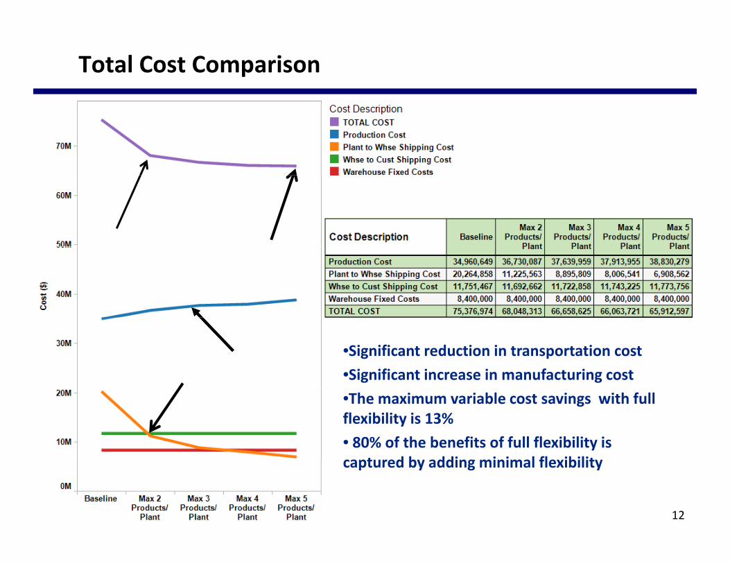
Total Cost Comparison
•Significant reduction in transportation cost •Significant increase in manufacturing cost•The maximum variable cost savings with full flexibility is 13%• 80% of the benefits of full flexibility is captured by adding minimal flexibilitycaptured by adding minimal flexibility
12

Impact of Changes in Demand Volume
Sensitivity analysis to changes above and below the forecast:
1.Growth for leading products (1 & 2) by 25% and slight decrease in demand for other products (5%). 2.Growth for the lower volume products (4 & 5) by 35% and slight decrease in demand for other products (5%).3.Growth of demand for the high potential product (3) by 100% and slight decrease in demand for other products (10%).
13

Impact of Changes in Demand Volume
Design Demand Satisfied Shortfall Cost/ Unit Avg Plant Utilization
Baseline 25 520 991 1 505 542 $ 2 94 91%
Demand Scenario 1
Baseline 25,520,991 1,505,542 $ 2.94 91%
Min Flexibility 27,026,533 0 $ 2.75 97%
Demand Scenario 2
Baseline 25,019,486 1,957,403 $ 2.99 91%
Min Flexibility 26,976,889 0 $ 2.75 96%
Demand Scenario 3
Baseline 23,440,773 4,380,684 $ 2.93 84%
Min Flexibility 27,777,777 43,680 $ 2.79 100%
14
y

Why 2‐Flexibility is so powerful?
Pittsburgh 3
2‐Flexibility
g
2
Modesto 5
Omaha
ProductPlant
Dayton 1
Amarillo 4
ProductPlant
• 2 Flexibility provides the benefits of full flexibility through the creation of a chain
15

Chaining Strategy (Jordan & Graves 1995)
• Focus: maximize the amount of demand satisfied• Simulation study
Full Flexibility
1 A
2 B
Short chains
1 A
2 B
Long chain1 A
2 B
3 C
y
3 C
4 D
5 E
3 C
4 D
5 E
3 C
4 D
5 E
~<
ProductPlant ProductPlant ProductPlant
6 F 6 F 6 F
16
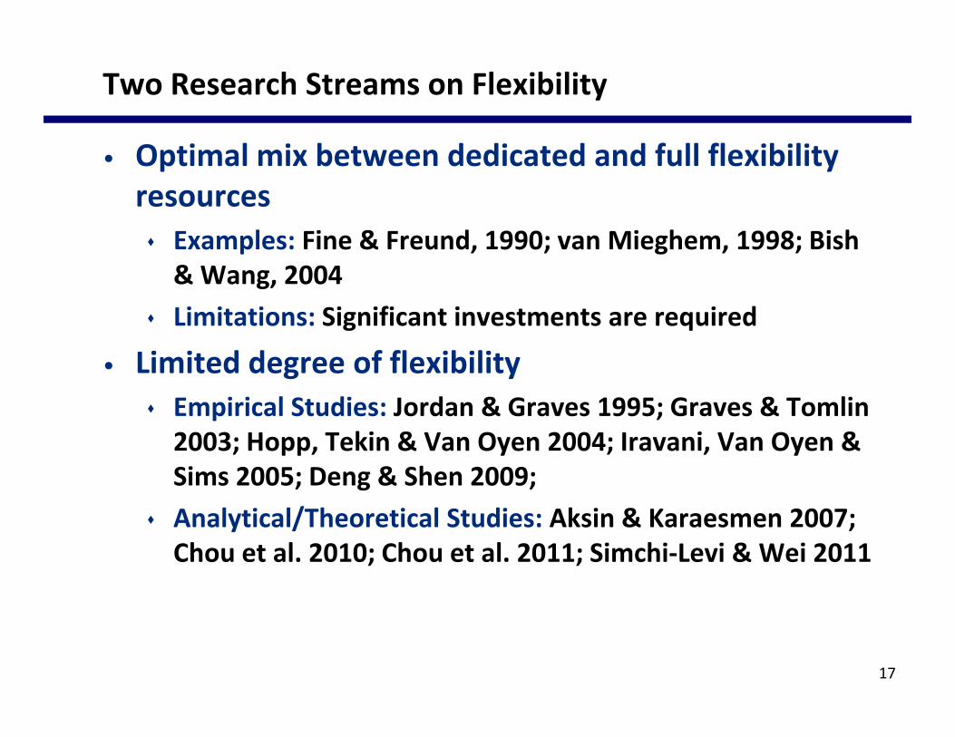
Two Research Streams on Flexibility
• Optimal mix between dedicated and full flexibility resources Examples: Fine & Freund, 1990; van Mieghem, 1998; Bish& Wang, 2004
Limitations: Significant investments are required Limitations: Significant investments are required
• Limited degree of flexibility Empirical Studies: Jordan & Graves 1995; Graves & TomlinEmpirical Studies: Jordan & Graves 1995; Graves & Tomlin 2003; Hopp, Tekin & Van Oyen 2004; Iravani, Van Oyen & Sims 2005; Deng & Shen 2009;
l i l/ h i l di k i & Analytical/Theoretical Studies: Aksin & Karaesmen 2007;Chou et al. 2010; Chou et al. 2011; Simchi‐Levi & Wei 2011
17

What We’ll Cover …
• Introduction to Flexibility• Model and Motivating Examples• Supermodularity in Long Chains• Additivity in Long Chainsy g• Summary
18

The Model: Flexible and Dedicated Arcs
Plants Products
• n plantsn plants• n products• Plant capacity = 1
Flexible ArcsDedicated Arcs
• Product demand I.I.D with mean 1
19

Model and the Performance Metric
For a fixed demand instance D, the sales for flexibility design A, P(D, A), is:
Given random demand D the performance of A is measured by
20
Given random demand D, the performance of A is measured by the expected sales of A, E[P(D, A)], (or [A])

A Motivating Example
1 1
Plants Products
Design PerformanceIncr.
PerformanceDedicated 5 6
1 1
2 2 Dedicated 5.6
3 3
4 4
5 5
6 6D d f h d t i IID d l
21
Demand for each product is IID and equals to 0.8, 1 or 1.2 with equal probabilities

A Motivating Example
1 1
Plants Products
Design PerformanceIncr.
PerformanceDedicated 5 6
1 1
2 2 Dedicated 5.6Add (1,2) 5.622 0.022
3 3
4 4
5 5
6 6
22

A Motivating Example
1 1
Plants Products
Design PerformanceIncr.
PerformanceDedicated 5 6
1 1
2 2 Dedicated 5.6Add (1,2) 5.622 0.022Add (2,3) 5.652 0.0303 3
4 4
5 5
6 6
23

A Motivating Example
1 1
Plants Products
Design PerformanceIncr.
PerformanceDedicated 5 6
1 1
2 2 Dedicated 5.6Add (1,2) 5.622 0.022Add (2,3) 5.652 0.030Add (3,4) 5.686 0.035
3 3
Add (3,4) 5.686 0.0354 4
5 5
6 6
24

A Motivating Example
1 1
Plants Products
Design PerformanceIncr.
PerformanceDedicated 5 6
1 1
2 2 Dedicated 5.6Add (1,2) 5.622 0.022Add (2,3) 5.652 0.030Add (3,4) 5.686 0.035
3 3
Add (3,4) 5.686 0.035Add (4,5) 5.724 0.03794 4
5 5
6 6
25

A Motivating Example
1 1
Plants Products
Design PerformanceIncr.
PerformanceDedicated 5 6
1 1
2 2 Dedicated 5.6Add (1,2) 5.622 0.022Add (2,3) 5.652 0.030Add (3,4) 5.686 0.035
3 3
Add (3,4) 5.686 0.035Add (4,5) 5.724 0.0379Add (5,6) 5.765 0.0403
4 4
5 5
6 6
26

A Motivating Example
1 1
Plants Products
Design PerformanceIncr.
PerformanceDedicated 5 6
1 1
2 2 Dedicated 5.6Add (1,2) 5.622 0.022Add (2,3) 5.652 0.030Add (3,4) 5.686 0.035
3 3
Add (3,4) 5.686 0.035Add (4,5) 5.724 0.0379Add (5,6) 5.765 0.0403Add (6,1) 5.842 0.077
4 4
( , )5 5
6 6
27

A Motivating Example
1 1
Observed by for example Hopp et al. (2004), Graves (2008)
Design PerformanceIncr.
PerformanceDedicated 5 6
1 1
2 2 Dedicated 5.6Add (1,2) 5.622 0.022Add (2,3) 5.652 0.030Add (3,4) 5.686 0.035
3 3
Add (3,4) 5.686 0.035Add (4,5) 5.724 0.0379Add (5,6) 5.765 0.0403Add (6,1) 5.842 0.077
4 4
( , )5 5
6 6
28
Note that the incremental benefit is increasing, and the largest increase occurs at the last arc.

Motivating Examples (Cont.)
1 11 1
2 2
3
2 2
3 3 3
4 4
3 3
4 4
5 55 5
6 66 6
Performance: 5 842Performance: 5 770
29
Performance: 5.842Performance: 5.770

What We’ll Cover …
• Introduction to Flexibility• Model and Motivating Examples• Supermodularity in Long Chains• Additivity in Long Chainsy g• Summary
30

Given Demand, a Long Chain and two Flexible Arcs and
where LC is the long chain we described previously
31
where LC is the long‐chain we described previously, while α and β are distinct arcs in the long‐chain.

Supermodularity of Flexible Arcs in a Long‐chain
32

P(uα,uβ,D) as a Maximum Weight Circulation Problem
S
Consider the following maximum weight circulation problem:
weighted arcs
u
1 D1
weighted arcs
1
Plant Nodes Product Nodes
uα1
1
D2
2
uβ
1
1
D3
D4
3
D4
This maximum weight circulation problem is equivalent to our
4
33
This maximum weight circulation problem is equivalent to our original formulation of P(uα,uβ,D).

Maximum Weight Circulation Problem
Definition.In a directed graph arcs α and β are said to be in series if thereIn a directed graph, arcs α and β are said to be in series if there
is no simple undirected cycle in which α and β have opposite directions.
For every cycle containing α and
Theorem (Gale, Politof 1981).Consider the maximum weight circulation problem correspond
αFor every cycle containing α and β, we have:
Consider the maximum weight circulation problem correspond to P(uα,uβ,D). If arcs α and β are in series, then P(uα,uβ,D) is supermodular.
β
34
β

Sketch of the Proof for Theorem 1
Fix any two flexible arcs α and β in the long‐chain. Consider any undirected cycle C which contains both α and β, if C does not contain S, the result is trivial; otherwise,
α
S 2k+1 arcs, directions of the arcs always alternating
35
β
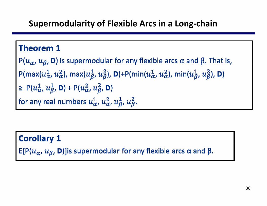
Supermodularity of Flexible Arcs in a Long‐chain
36
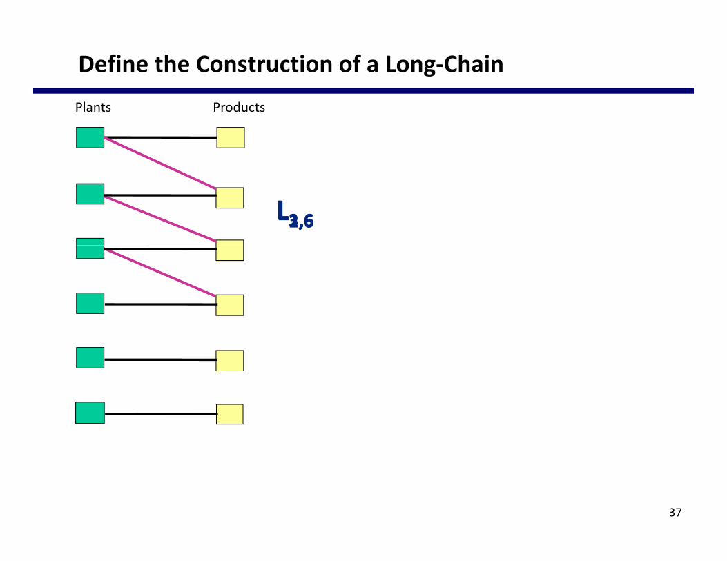
Define the Construction of a Long‐ChainPl t P d tPlants Products
L2,6L3,6L1,6
37

Define the Construction of a Long‐ChainPl t P d tPlants Products
L4,6
38
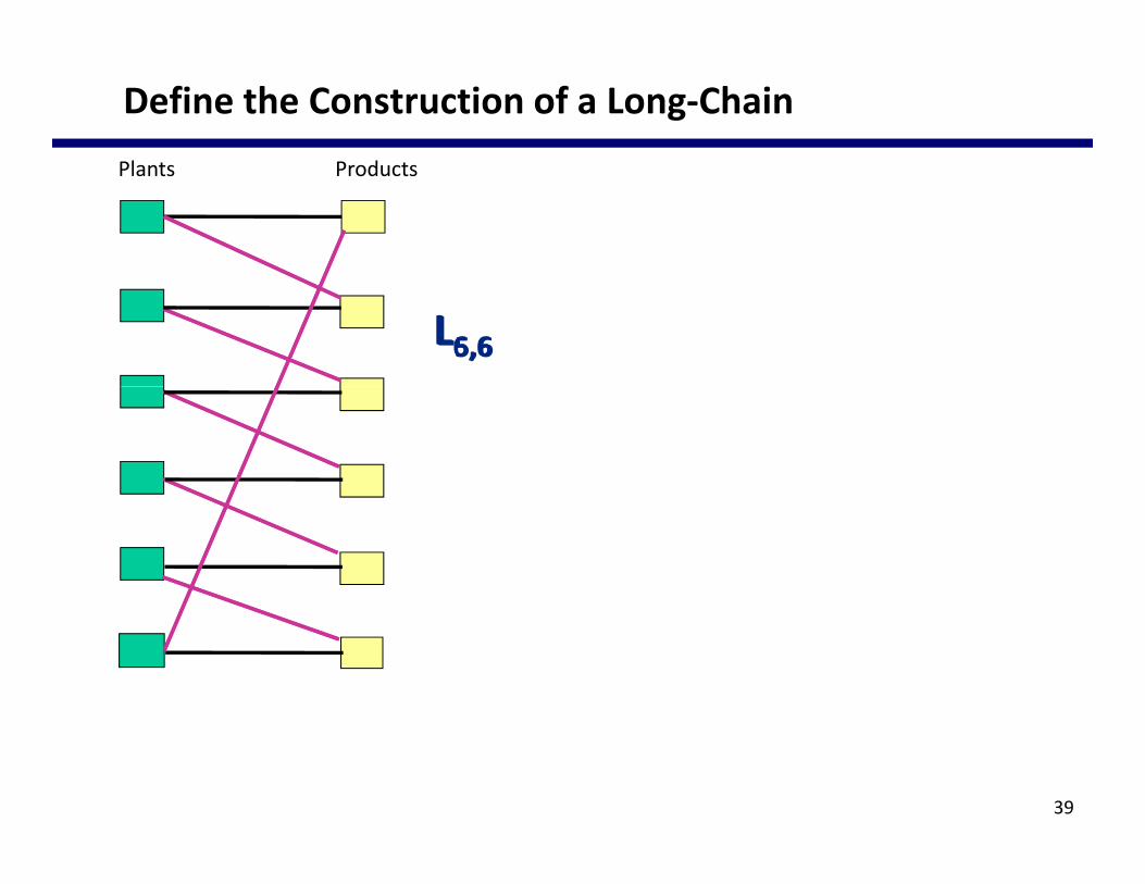
Define the Construction of a Long‐ChainPl t P d tPlants Products
L5,6L6,6
39

How supermodulrity explains the power of the Long Chain?
1 D1 D1D1 D1
By Theorem 1 we have:
2 D2
3 D
+ ≥ D2
D
+1
D2
D
1
D2
DD3
4 D4
D3
D4
D3
D4
D3
D4
α β
With u¹ =1 u¹ =0 and u² =0 u² =1
D1D1 D1 D1
With u¹α=1, u¹β =0 and u α =0, u β=1
D2
D3
D2
D3
‐ ≥ D2
D3
‐1
D2
D3
D4
3
D4
3
D4
D3
D4

The Power of the Long Chain
Corollary 2Suppose the demand for each product is IID, thenSuppose the demand for each product is IID, then E[P(D, Lk+1,n)] – E[P(D, Lk,n)]≥ E[P(D, Lk,n)] – E[P(D, Lk‐1,n)] for any 1 ≤ k ≤ n‐1.
For example, in expectation, we have
E[P(D L )] E[P(D L )] E[P(D L )] E[P(D L )]
D1
D2
D1
D
D1
D
D1
E[P(D,L4,4)] E[P(D,L3,4)] E[P(D,L3,4)] E[P(D,L2,4)]
D2
D3
D
‐ ≥D2
D3
D2
D3
‐ D2
D3
41
D4 D4 D4 D4

What We’ll Cover …
• Introduction to Flexibility• Model and Motivating Examples• Supermodularity in Long Chains• Additivity in Long Chainsy g• Summary
42

Characterizing the Sales of the Long Chain
1 11 1
Example: For n =4, i=21
2 2
1
P(D LC/{α }) ( /{ β })P(D LC)
1 1
2 2
3 3 3 3
P(D, LC/{αi}) P(D, LC/{αi, αi‐1, βi}) P(D, LC)
43
4 4 4 4

Illustrating the Characterization
1 1
2 2 2 2‐1 1
3 3 3 3
+2 2
1 1
2 2
1 1
‐=
3 3
3 3 3 3
+1 1
2 2
1 1
2 2‐
44
3 3

The ``Dummy’’ Arc in Long Chain
Lemma 1 Suppose P(D, LC) = P(D, LC /{αi*}) for some i*, then
P(D, LC/{αi}) = P(D, LC/{αi ,αi*})P(D, LC/{αi ,αi‐1 ,βi}) = P(D, LC/{αi ,αi‐1 ,βi ,αi*})
where α (i i+1) for i 1 n 1 α (n 1) and β (i i) for i 1 nwhere αi=(i,i+1) for i=1,…,n‐1, αn=(n,1) and βi=(i,i) for i=1,..n.
Proof: Lemma 1 follows by the supermodularity result stated in y p yTheorem 1.
45

“Proof’’ for the Theorem 2
1 1
2 2 2 2‐1 1
3 3 3 3
+2 2
1 1
2 2
1 1
‐=
3 3
3 3 3 3
+1 1
2 2
1 1
2 2‐
46
3 3

The Characterization In Expectation
1 1
2 2 2 2‐In expectation,
1 1
3 3 3 3
+= =
2 2
1 1
2 2
1 1
‐= 3X ( )3 3
3 3 3 3
+
= =
E[P(D,L2,3)] E[P(D,L1,2)]
( )
1 1
2 2
1 1
2 2‐E[P(D,L3,3)]
Theorem 3 (Characterizing the Performance of Long Chain)
47
3 3Theorem 3 (Characterizing the Performance of Long Chain)For IID demand, E[P(D,Ln,n)] = n(E[P(D,Ln‐1,n)]– E[P(D,Ln‐2,n‐1)])

The “Impact” of Theorem 2
Corollary 3 (Risk Pooling of Long Chain)Suppose the demand for each product is IID and capacity for each plant is 1, then in a n by n product plant system, we have E[P(D,Ln+1,n+1)]/(n+1) ≥ E[P(D,Ln,n)]/n
Corollary 4 (Optimality of Long Chain)In an n product‐plant system, if the demand for each product is IID and capacity for each plant is 1, the long chain is always the optimal 2‐flexibility system.
Corollary 5 (Computing the Performance of Long Chain)If D1 has the support set {k/N : k=0,1,2,…}, then E[P(D, Ln n)] can
48
1 pp { / , , , }, [ ( , n,n)]be computed with matrix multiplications in O(nN2) operations.

Plotting the Fill Rate of Long Chain and Full Flexibility
1
0.9
0.95
Full Flexibility
0.8
0.85FullFlexibilityLongChainLongChain/Full
0.7
0.75
1 6 11 16 21 26
Distribution of D1 is uniformly distributed on
1 6 11 16 21 26
49
1 y{1/10, 2/10, …, 20/10}.

Risk Pooling of the Long Chain
Corollary 3 (Risk Pooling of Long Chain)Under IID demand, E[P(D,Ln+1 n+1)]/(n+1) ≥ E[P(D,Ln n)]/n.
Theorem 4 (Exponential Decrease of Risk Pooling)
, [ ( , n+1,n+1)]/( ) [ ( , n,n)]/
Theorem 4 (Exponential Decrease of Risk Pooling)Under IID demand, limn→∞log(E[P(D,Ln+1 n+1)]/(n+1)‐E[P(D,Ln n)]/n) ≤ nK, n→ g( [ ( , n+1,n+1)]/( ) [ ( , n,n)]/ ) ,for some negative constant K.
Theorem 4 implies that in a system with very large size, a collection of several large chains is just as good as a single long chain.
50

Long Chain vs Full Flexibility
The first inequality of Theorem 4 shows that the gap between the fill rate of full flexibility that of the long chain is increasing.y g g
51
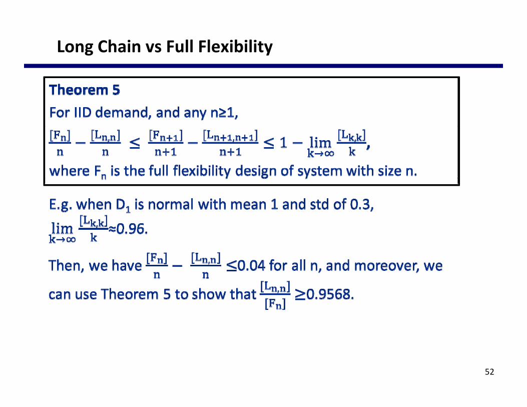
Long Chain vs Full Flexibility
52
What We’ll Cover …
• Introduction to Flexibility• Model and Motivating Examples• Supermodularity in Long Chains• Additivity in Long Chainsy g• Summary
53

Key Observations
• The age of Flexibility has arrived The Decade of the 80’s: Significant disappointment inThe Decade of the 80 s: Significant disappointment in industry with flexibility (Jaikumar, 1986)
The Decade of the 90’s and early 2000: Higher flexibility in the automotive industry (Van Biesebroeck 2004)the automotive industry (Van Biesebroeck, 2004)
Today: More and more companies in diverse industries invest in various types of flexibility (Simchi‐Levi, 2010)
• More research is needed to help bl h d d l Establish design guidelines
Analyze more realistic business settings (multi‐stage, variability up‐stream, information sharing)
54
y p , g) Identify the level of flexibility required
