managing high-availability and elasticity in a cluster ... · managing high-availability and...

Managing High-Availability and Elasticity in a Cluster

Environment

Neha Pawar

A Thesis

in

The Department

of

Computer Science and Software Engineering

Presented in Partial Fulfilment of the Requirements

for the Degree of Master of Applied Science (Software Engineering) at

Concordia University

Montreal, Quebec, Canada

August, 2014

© Neha Pawar, 2014 CONCORDIA UNIVERSITY

School of Graduate Studies

This is to certify that the thesis prepared

By: Neha Pawar

Entitled: Managing High-Availability and Elasticity in a Cluster Environment

and submitted in partial fulfillment of the requirements for the degree of

Master of Applied Science (Software Engineering)

complies with the regulations of the University and meets the accepted standards with respect to

originality and quality.

Signed by the final examining committee:

Dr. R. Jayakumar Chair

Dr. D. Goswami Examiner

Dr. J. Paquet Examiner

Dr. F. Khendek Supervisor

Dr. M. Toeroe Co-Supervisor

Approved by Dr. V. Haarslev

Chair of Department or Graduate Program Director

Dr. C. Trueman

Dean of Faculty

Date September 2014

Abstract

Managing High-Availability and Elasticity in a Cluster Environment

Neha Pawar

Cloud computing is becoming popular in the computing industry. Elasticity and availability are

two features often associated with cloud computing. Elasticity is defined as the automatic

provisioning of resources when needed and de-provisioning of resources when they are not

needed. Cloud computing offers the users the option of only paying for what they use and

guarantees the availability of virtual infrastructure (i.e. virtual machines). The existing cloud

solutions handle both elasticity and availability at the virtual infrastructure level through the

manipulation, restart, addition and removal of virtual machines (VMs) as required. These

solutions equate the application and its workload to the VMs that run the application. High-

availability applications are typically composed of redundant resources, and recover from

failures through failover mostly managed by a middleware. For such applications, handling

elasticity at the virtual infrastructure level through the addition and removal of VMs is not

enough, as the availability management in application level will not make use of additional

resources. This requires new solutions that manage both elasticity and availability in application

level. In this thesis, we provide a solution to manage the elasticity and availability of applications

based on a standard middleware defined by the Service Availability Forum (SA Forum). Our

solution manages application level elasticity through the manipulation of the application

configuration used by the middleware to ensure service availability. For this purpose we

introduce a third party, ‘Elasticity Engine’ (EE), that manipulates the application configuration

used by the SA Forum middleware when a workload changes. This in turn triggers the SA Forum

iii

middleware to change the workload distribution in the system while ensuring service availability.

We explore the SA Forum middleware configuration attributes that play a role in elasticity

management, the constraints applicable to them, as well as their impact on the load distribution.

We propose an overall architecture for availability and elasticity management for an SA Forum

system. We design the EE architecture and behavior through a set of strategies for elasticity. The

proposed EE has been implemented and tested.

iv

Acknowledgements

I would like to thank my supervisor, Prof. Ferhat Khendek, for believing in me and giving me the

opportunity to pursue my thesis under his supervision. The thesis would not have been possible

without his support and encouragement.

I would also like to thank my co-supervisor Dr. Maria Toeroe (Ericsson Canada Inc.) for sharing

her immense knowledge in the domain of Service Availability and for providing guidance which

helped me to overcome the challenges in completing this thesis.

My special thanks to my family and friends who supported me selflessly. I would also like to

offer special thanks to my colleagues in the MAGIC team for their friendship and for creating a

pleasant work atmosphere.

I am also grateful to Concordia University and Ericsson Canada for offering their facilities and

resources.

This work has been partially supported by Natural Sciences and Engineering Research Council

of Canada (NSERC), and Ericsson Software Research and Concordia University as part of the

Industrial Research Chair in Model Based Software Management.

v

Table of Contents

List of Figures ................................................................................................................................ ix

List of Tables ............................................................................................................................... xiii

List of Acronyms ......................................................................................................................... xiv

Chapter 1 - Introduction .................................................................................................................. 1

1.1 Thesis Motivation .............................................................................................................. 3

1.2 Thesis Contributions .......................................................................................................... 5

1.3 Thesis Organization ........................................................................................................... 6

Chapter 2 - Background and Related Work .................................................................................... 7

2.1 SA Forum Specifications ................................................................................................... 7

2.2. Availability Management Framework (AMF) ................................................................. 8

2.2.1 Logical Entities ................................................................................................... 8

2.3 Information Model Management (IMM) ........................................................................ 15

2.3.1 Information Model Organization ...................................................................... 17

2.3.2 Object Management .......................................................................................... 19

2.3.3 Object Implementer Management .................................................................... 21

2.4 Related Work ................................................................................................................... 23

Chapter 3 - Elasticity in Availability Management Framework ................................................... 26

3.1 Elasticity Related Attributes in an AMF Configuration .................................................. 26

vi

3.2 Types of workload changes in an AMF Configuration ................................................... 32

3.2.1 Single-SI Type workload changes .................................................................... 32

3.2.2 Multiple-SI type workload changes .................................................................. 33

3.3 Summary ......................................................................................................................... 34

Chapter 4 - Overall Architecture and Elasticity Engine ............................................................... 35

4.1 Overall architecture for HA and elasticity management ................................................. 35

4.2 The Elasticity Engine Architecture ................................................................................. 36

4.3 Elasticity Engine Strategies ........................................................................................ 39

4.3.1 Workload increase ............................................................................................ 40

4.3.2 Workload decrease ........................................................................................... 43

4.3.3 Buffer management .......................................................................................... 46

4.3.4 Cluster Level Adjustments ............................................................................... 49

4.4 Elasticity Engine Algorithms .......................................................................................... 50

4.4.1 Workload increase algorithms .......................................................................... 50

4.4.2 Workload decrease algorithms ......................................................................... 58

4.4.3 Buffer Management algorithms ........................................................................ 64

4.5 Summary ......................................................................................................................... 67

Chapter 5 - A Prototype of the Elasticity Engine ......................................................................... 69

5.1 The EE Prototype Architecture ....................................................................................... 69

5.2 Experiment Test-bed Set-up ............................................................................................ 72

vii

5.3 A Case Study ................................................................................................................... 73

5.4 Experiments with the EE Prototype Tool ........................................................................ 74

5.4.1 Workload increase ............................................................................................ 74

5.4.2 Workload decrease ........................................................................................... 82

5.4.3 Cluster Level Adjustments ............................................................................... 88

5.5 Summary ......................................................................................................................... 91

Chapter 6 - Conclusion and Future Work ..................................................................................... 92

6.1 Conclusion ....................................................................................................................... 92

6.2 Future Work .................................................................................................................... 93

Reference ...................................................................................................................................... 95

Appendix ....................................................................................................................................... 98

viii

List of Figures

FIGURE 1 - AN OVERVIEW OF THE SA FORUM SERVICES [9] ............................................................. 7

FIGURE 2 - AMF SYSTEM MODEL [4] .............................................................................................. 9

FIGURE 3 - EXAMPLE OF 2N REDUNDANCY MODEL ........................................................................ 12

FIGURE 4 - EXAMPLE OF N+M REDUNDANCY MODEL .................................................................... 12

FIGURE 5 - EXAMPLE OF N-WAY REDUNDANCY MODEL ................................................................. 13

FIGURE 6 - N-WAY ACTIVE REDUNDANCY MODEL .......................................................................... 14

FIGURE 7 - EXAMPLE OF NO-REDUNDANCY REDUNDANCY MODEL ................................................ 14

FIGURE 8 - IMM SERVICE INTERFACE [7] ...................................................................................... 16

FIGURE 9 - EXAMPLE OF THE INFORMATION MODEL ...................................................................... 18

FIGURE 10 - CONFIGURATION CHANGE BUNDLE FOR A SAMPLE APPLICATION [7] ........................ 21

FIGURE 11 - EXAMPLE OF WEB SERVICE APPLICATION ................................................................. 28

FIGURE 12 - EXAMPLE FOR SINGLE-SI TYPE WORKLOAD CHANGE ............................................... 33

FIGURE 13 - EXAMPLE OF MULTIPLE-SI TYPE WORKLOAD CHANGE ............................................. 34

FIGURE 14 - OVERALL ARCHITECTURE FOR HA AND ELASTICITY MANAGEMENT WITH AMF ...... 36

FIGURE 15 - THE ARCHITECTURE OF EE ........................................................................................ 38

FIGURE 16 - EE’S SEQUENCE DIAGRAM ......................................................................................... 39

FIGURE 17 - SPREADING THE SI WORKLOAD .................................................................................. 41

FIGURE 18 - DISTRIBUTING THE SIS OVER MORE SUS ................................................................... 42

FIGURE 19 - PRIORITIZING THE SU ON THE LEAST LOADED NODE ................................................. 43

FIGURE 20 - MERGING THE SI WORKLOAD ..................................................................................... 44

FIGURE 21 - RE-GROUPING THE SIS TO LESS SUS OF THE SG ......................................................... 45

ix

FIGURE 22 - PRIORITIZING THE NODES THAT SERVE OTHER SIS ...................................................... 46

FIGURE 23 - BUFFER MANAGER ..................................................................................................... 49

FIGURE 24 - CLUSTER LEVEL ADJUSTMENTS ................................................................................. 50

FIGURE 25 - FLOW-CHART: SPREADING THE SI’S WORKLOAD (N-WAY-ACTIVE REDUNDANCY

MODEL) .................................................................................................................................. 52

FIGURE 26 - FLOW-CHART: DISTRIBUTING SIS OVER MORE SUS (N+M & N-WAY REDUNDANCY

MODELS) ................................................................................................................................ 55

FIGURE 27 - FLOWCHART: PRIORITIZING SU ON THE LEAST LOADED NODE (2N & NO

REDUNDANCY MODELS) ......................................................................................................... 57

FIGURE 28 - FLOWCHART: MERGING THE SI WORKLOAD (N-WAY-ACTIVE REDUNDANCY MODEL)

............................................................................................................................................... 59

FIGURE 29 - FLOWCHART: RE-GROUPING THE SIS ON LESS SUS (N+M & N-WAY REDUNDANCY

MODELS) ................................................................................................................................ 62

FIGURE 30 - FLOWCHART: PRIORITIZING NODES THAT SERVE OTHER SIS (2N & NO REDUNDANCY

MODELS) ................................................................................................................................ 64

FIGURE 31 - FLOWCHART: BUFFER MANAGER (RESERVATION OF RESOURCES) ............................ 66

FIGURE 32 - FLOWCHART: BUFFER MANAGER (FREEING RESERVED RESOURCES) ........................ 67

FIGURE 33 - EE PROTOTYPE TOOL ARCHITECTURE ....................................................................... 70

FIGURE 34 – A GUI FOR RENDERING AN AMF CONFIGURATION .................................................... 71

FIGURE 35 – SYSTEM CONFIGURATION FOR THE CASE STUDY ....................................................... 74

FIGURE 36 - ‘SAFSG=AMFDEMO,SAFAPP=AMFDEMO1’ SG OBJECT BEFORE THE EE ACTION ....... 75

FIGURE 37 - ‘SAFSI=AMFDEMO,SAFAPP=AMFDEMO1’ SI OBJECT BEFORE THE EE ACTION ........ 76

x

FIGURE 38 - SYSTEM CONFIGURATION AFTER EE AND AMF ACTIONS FOR THE WORKLOAD

INCREASE IN A SG WITH N-WAY- ACTIVE REDUNDANCY MODEL .......................................... 77

FIGURE 39 - ‘SAFSG=AMFDEMO,SAFAPP=AMFDEMO1’ SG OBJECT AFTER THE EE ACTION ....... 78

FIGURE 40 - ‘SAFSI=AMFDEMO,SAFAPP=AMFDEMO1’ SI OBJECT AFTER THE EE ACTION .......... 78

FIGURE 41 - ‘SAFSG=AMFDEMO,SAFAPP=AMFDEMO2’ SG OBJECT BEFORE THE EE ACTION ..... 79

FIGURE 42 - ‘SAFSI=AMFDEMOSI,SAFAPP=AMFDEMO2’ AND

‘SAFSI=AMFDEMOSI1,SAFAPP=AMFDEMO2’ OBJECT BEFORE THE EE ACTION ................... 79

FIGURE 43 - SYSTEM CONFIGURATION AFTER EE AND AMF ACTIONS FOR WORKLOAD INCREASE

IN A SG WITH N+M REDUNDANCY MODEL ............................................................................ 82


FIGURE 45 - SYSTEM CONFIGURATION AFTER EE AND AMF ACTIONS FOR A WORKLOAD

DECREASE IN A SG WITH THE N-WAY- ACTIVE REDUNDANCY MODEL .................................. 84


FIGURE 47 - ‘SAFSI=AMFDEMO,SAFAPP=AMFDEMO1’ SG OBJECT AFTER THE EE ACTION ........ 85

FIGURE 48 - SYSTEM CONFIGURATION AFTER EE AND AMF ACTIONS FOR A WORKLOAD

DECREASE IN AN SG WITH N+M REDUNDANCY MODEL ........................................................ 88

FIGURE 49 - ‘SAFSG=AMFDEMO,SAFAPP=AMFDEMO2’ SG AFTER THE EE ACTION ..................... 88

FIGURE 50 - SYSTEM CONFIGURATION TO TEST CLUSTER LEVEL ADJUSTMENT ............................ 89

FIGURE 51 - SYSTEM CONFIGURATION AFTER EE AND AMF ACTION FOR CLUSTER LEVEL

ADJUSTMENT .......................................................................................................................... 91

FIGURE 52 - SYSTEM CONFIGURATION OF SGS WITH 2N REDUNDANCY MODEL BEFORE CCB

IMPLEMENTATION ................................................................................................................... 98

xi

FIGURE 53 - SYSTEM CONFIGURATION OF SGS WITH 2N REDUNDANCY MODEL AFTER CCB

IMPLEMENTATION (WORKLOAD INCREASE) ......................................................................... 100

FIGURE 54 - SYSTEM CONFIGURATION OF SGS WITH 2N REDUNDANCY MODEL AFTER CCB

IMPLEMENTATION (WORKLOAD DECREASE) .......................................................................... 102

FIGURE 55 - SYSTEM CONFIGURATION OF SG WITH N-WAY REDUNDANCY MODEL BEFORE CCB

IMPLEMENTATION (SINGLE-SI) ............................................................................................. 103

FIGURE 56 - SYSTEM CONFIGURATION OF SG WITH N-WAY REDUNDANCY MODEL AFTER CCB

IMPLEMENTATION (WORKLOAD INCREASE) ......................................................................... 105

FIGURE 57 - SYSTEM CONFIGURATION OF SG WITH THE N-WAY REDUNDANCY MODEL WITH CCB

IMPLEMENTATION (WORKLOAD DECREASE) ........................................................................ 106


IMPLEMENTATION (MULTIPLE-SI WORKLOAD INCREASE) ................................................... 107

FIGURE 59 - SYSTEM CONFIGURATION OF SG WITH N-WAY REDUNDANCY MODEL AFTER CCB

IMPLEMENTATION (MULTIPLE-SI WORKLOAD INCREASE) ..................................................... 108


IMPLEMENTATION (MULTIPLE-SI WORKLOAD DECREASE) .................................................... 109

FIGURE 61 – SYSTEM CONFIGURATION OF SG WITH THE N-WAY REDUNDANCY MODEL AFTER CCB

IMPLEMENTATION (MULTIPLE-SI WORKLOAD DECREASE) .................................................. 110

xii

List of Tables

TABLE 1 - AMF ELASTICITY RELATED ATTRIBUTES OF SERVICE PROVIDER SIDE ENTITIES ......... 29

TABLE 2- AMF ELASTICITY RELATED ATTRIBUTES OF SERVICE SIDE ENTITIES .............................. 31

TABLE 3 - INVESTIGATION SCENARIOS......................................................................................... 111

xiii

List of Acronyms

ActSUs SaAmfSGPrefNumStandbySUs

AIS Application Interface Specification

AMF Availability Management Framework

API Application Programming Interface

AS Application Server

AssSUs saAmfSGNumPrefAssignedSUs

CCB Configuration Change Bundle

CLM Cluster Membership Service

CompMaxActCSIs saAmfCompNumMaxActiveCSIs

CompMaxStdCSIs saAmfCompNumMaxStandbyCSIs

CSI Component Service Instance

DN Distinguished Name

EE Elasticity Engine

GUI Graphical User Interface

HA High Availability

HPI Hardware Platform Interface

IM Information Model

IMM Information Model Management

InsSUs saAmfSGNumPrefInserviceSUs

LDAP Lightweight Directory Access Protocol

xiv

MaxStdSIperSU saAmfSGMaxStandbySIsperSU

OCL Object Constraint Language

OI-API Object Implementers API

OM-API Object Management API

PLM Platform Management Service

RDN Relative Distinguished Name

RM Redundancy Model

SA Forum Service Availability Forum

SG Service Group

SI Service Instance

SIAssgmnts saAmfSIPrefActiveAssignments

SLA Service Level Agreement

SMF Service Management Framework

SU Service Unit

TIPC Transparent Inter-Process Communication

UML Unified Modeling Language

URL Uniform Resource Locator

VM Virtual Machine

xv

Chapter 1 - Introduction

This chapter introduces topics discussed throughout this thesis, the motivations behind

this thesis and contributions of the thesis. In this chapter we also present the organization of the

thesis.

Nowadays, the world depends mostly on computers and the services that computer

applications provide. The growth in the use of computers has resulted in high demand and new

requirements from the users. The users expect services to be always available and in reach all the

time, in other words, the users want services that are highly available. Service availability is

defined as the percentage of time the application is running and its services are provided [1].

High Availability (HA) is defined as the availability of a service at least 99.999% [1] of

the time. Highly available systems have become a necessity in almost all the domains ranging

from banking, telecommunications, and web services to mission critical systems [2]. HA in cloud

computing is a big challenge. However, availability is an implicit expectation of cloud systems.

Elasticity, on the other hand, is one of the key features of cloud computing that makes cloud

computing economically attractive and therefore drives its wide-spreading deployment. Elasticity

is defined as the provisioning or de-provisioning of resources according to the workload

variations of application services allowing for a “pay-as-you-go” charging model [3].

Current cloud solutions handle both availability and elasticity at the virtual infrastructure

level. They manage availability by starting and restarting virtual machines (VMs) when current

executing VM fails; and similarly when workload changes VMs are added and removed

accordingly. This approach equates the application and its workload to the VMs running the

1

application. It also assumes that the application starts with the VM, it is stateless, and the VMs

running the same application share the load.

These assumptions are not necessarily true when we consider applications that provide

highly available services such as telecom applications. HA applications generally run in a cluster

and their availability is managed by a middleware application. This middleware maintains state-

full redundant resources of the application which act as standbys to protect their active peers.

The middleware performs error recovery by controlling the life-cycle of the application resources

for which it requires a configuration describing the organization of the application.

When we consider elasticity in this context, removing VMs due to decreased workload

could be considered by the availability management as a failure of the VM and therefore handled

as such. Furthermore, mere addition of new VMs in the case of workload increase will not

necessarily lead to the utilization of the new VMs by the application level, potentially causing

repeated triggers for elasticity management at the infrastructure level. Repeated triggers for the

same workload change may also happen for different VMs due to the availability management

performing the switch or a failover at the application level, i.e. in this context the workload

cannot be associated with the given VM. We need a new solution that coordinates the elasticity

and the availability at an application level.

In this thesis we provide a solution to manage elasticity and availability of applications

based on the Availability Management Framework (AMF) [4] of the Service Availability Forum

(SA Forum) [5] designed to maintain service availability. The SA Forum has defined a set of

middleware Application Programming Interface (API) specifications to facilitate the

development of carrier grade and mission critical applications. The SA Forum specifications

have been implemented by OpenSAF [6], an open source project.

2

1.1 Thesis Motivation

As mentioned before the HA applications like telecom applications are composed of

redundant resources in cluster and their availability is managed by a middleware. The

middleware defined by SA Forum is a proven solution for service availability in the context of

cluster computing. Enabling elasticity within the SA Forum’s middleware will position SA

Forum middleware as a potential solution for managing HA applications in the cloud.

In the SA Forum middleware, AMF is the most important service responsible for the HA

of the services of the applications. It maintains the availability of services of application by

managing and coordinating redundant resources of these applications.

The redundancy and the logical organization of the applications are described for AMF in

a configuration, which is part of the information model maintained by the SA Forum Information

Model Management (IMM) [7] service. IMM provides an administrative API that allows the

system administration to manipulate the information model, including the AMF configuration.

After manipulation, IMM notifies entities such as AMF which implement the modifications.

In an AMF configuration there are two types of entities: entities that represent the

application services and entities that are actually capable of providing the services, which

represent the resources. AMF assigns each service entity to one or more service provider entity.

When the service provider entity fails AMF automatically moves the assignments of the failed

service provider entity to another healthy service provider entity. The actual workload the service

entities assignment impose on the service provider entities may vary over time, it may potentially

increase or decrease within a wide range.

AMF is a proven solution for service availability in the context of cluster computing,

however it was not explicitly designed to handle elasticity for cloud computing. AMF allows for

3

the manipulation of its configuration. AMF configuration can be manipulated to trigger AMF

actions that increase the resources available for a service entity when its workload increases and

vice versa when it decreases. This gives us motivation to present a solution which enables both

elasticity and availability within AMF configurations.

4

1.2 Thesis Contributions

In this thesis, we present how an AMF configuration can be used to trigger AMF actions

that increase the resources available for a service entity when its workload increases and

decrease resources available for the service entity when its workload decreases. We propose an

Elasticity Engine (EE) that enables elasticity in a configuration designed for service availability,

therefore achieving both simultaneously. It reacts to workload change variations by modifying

the AMF configuration that triggers AMF to dynamically provision or de-provision resources. In

this thesis we:

1. Define two types of workload changes in an AMF configuration to characterize the

potential changes in workload.

2. Define an overall architecture for HA and elasticity management using the SA Forum

middleware.

3. Define the architecture and behavior of the EE through different strategies to increase and

decrease workloads including buffer (reserved resources) management to enable

elasticity.

4. Implement the EE and perform some experiments.

In our thesis we have focused on AMF managed applications. AMF maintains

availability of the applications as long as the AMF configuration remains valid. Thus in our

thesis we have assumed that AMF will maintain availability and our solution will enable

elasticity within AMF. We also assume that the workload changes of the applications are

determined by an external application that is the workload monitor. The workload monitor

only signals to our EE when the workload increases beyond or decreases below certain

threshold.

5

1.3 Thesis Organization

The thesis is organized into six chapters. In Chapter 2 we provide the necessary

background information on the SA Forum middleware and discuss related work. In Chapter 3,

we investigate the elasticity feature in AMF configurations. Chapter 4 presents our overall

architecture for HA and elasticity management with the SA Forum middleware. It elaborates on

the architecture of the EE and its behavior including the elasticity strategies. Chapter 5 presents

our prototype tool and experiments. In Chapter 6 we summarize our work and discuss potential

future work.

6

Chapter 2 - Background and Related Work

In this chapter we introduce the SA Forum specifications, specifically the AMF service

and the IMM service, followed by a review of related work.

2.1 SA Forum Specifications

The objective of the SA Forum is to define standard interfaces that facilitate the

development of carrier-grade and mission critical applications and systems [5]. It is a consortium

formed by telecommunication and computing companies that defines specifications for the

standardization of high availability platforms. OpenSAF middleware [6] is an open source

implementation of the SA Forum specifications.

Figure 1 - An overview of the SA Forum services [8]

The SA Forum services are categorized into: the Hardware Platform Interface (HPI) [8]

and the Application Interface Specification (AIS) [9]. The main objective of HPI is to provide

standardized interfaces to manage hardware platforms. The HPI specifications contain data

7

structures and functional definitions that are used to communicate with other platforms or

systems [5] [8]. The main objective of AIS is to provide standardized APIs for middleware

functions typically required by HA applications. These specifications consist of different

middleware services among which we will be focusing on the AMF [4] service and the IMM [7]

service that are more relevant to this thesis. Figure 1 gives an overview of the SA Forum

services.

2.2. Availability Management Framework (AMF)

AMF [4] manages the availability of services provided by an application through the

management and coordination of its redundant resources, and performing some recovery and

repair actions in case of a failure. To do so, AMF requires a configuration of the application that

represents the application from AMF perspective and describes the different entities composing

it and their relations.

2.2.1 Logical Entities

The AMF specification [4] defines a set of logical entities. These logical entities are

shown in Figure 2. We describe the logical entities in this section.

8

Figure 2 - AMF System Model [4]

• Component:

It is the logical entity that represents a set of resources to AMF. This set of resources can

include hardware resources, software resources, or a combination of the two. It is the

smallest logical entity on which AMF performs error detection and isolation, recovery

and repair [4]. Components are categorized into SA-Aware and Non-SA-Aware.

9

SA-Aware:

This type of component is integrated and controlled by AMF directly. The

component registers itself using AMF APIs [4]. It also implements the interfaces

and callback functions that provide means to communicate between AMF and the

components.

Non-SA-Aware:

This type of component cannot directly communicate with AMF. A mediator

component is required to link AMF and the Non-SA-Aware components. The

mediator is a proxy component. The Non-SA-Aware component is the proxied

component and it can communicate with AMF only through a proxy component

that is SA-Aware.

• Component Type:

A component type defines the list of attribute values that are shared by components of the

same type.

• Service Unit (SU):

It is a logical entity that aggregates a set of components combining their individual

functionalities to provide a higher level of service. SUs can contain any number of

components, but a particular component can be configured in only one SU.

• Service Unit Type:

A service unit type defines a list of component types and for each of the component

types, the number of components that a SU of this type may accommodate. All SUs of

the same type share the attribute values defined in the service unit type configuration.

10

• Component Service Instance (CSI):

CSI represents the workload that AMF can dynamically assign to a component.

• Component Service Type:

A component service type defines the list of attribute names that are shared by all the

CSIs of the same type.

• Service Instance (SI):

SI aggregates all CSIs to be assigned to the SU to provide a higher level of service. A SI

can contain multiple CSIs, but a particular CSI can be configured in only one SI.

• Service Type:

A service type defines the list of component service types from which its SIs can be built.

• Service Group (SG):

A set of redundant SUs is organized into a SG to protect a particular set of SIs. AMF

manages the service availability by assigning active and standby workloads to redundant

SUs of each SG. Any SU of the SG must be able to take an assignment for any SI of this

set. The redundant SUs collaborate with each other depending on the type of the

redundancy model of the SG. AMF defines five redundancy models:

2N Redundancy Model:

A SG of 2N redundancy model has at most one SU that handles active

assignments and at most one SU that handles standby assignments of all SIs

protected by SG. If there are other SUs of the SG, they are spare SUs. Each SI has

only one active assignment and one standby assignment. A SU cannot handle

active assignments for some SIs and handle standby assignments for some other

SIs at the same time (Figure 3).

11

Figure 3 - Example of 2N redundancy model

N+M Redundancy Model:

A SG of N+M redundancy model allows ‘N’ SUs to handle active assignments

and ‘M’ SUs to handle standby assignments for all SIs protected by SG. Each SI

will have only one active assignment and one standby assignment. A SU cannot

handle active assignments for some SIs and standby assignments for some other

SIs at the same time (Figure 4).

Figure 4 - Example of N+M redundancy model

12

N-way Redundancy Model:

A SG of N-way redundancy model allows a SU to handle active and standby

assignments of different SIs at the same time. Each SI protected by an SG of N-

way redundancy will have only one active assignment and can have one or more

standby assignments (Figure 5).

Figure 5 - Example of N-way redundancy model

N-way-Active Redundancy Model:

A SG of an N-way-Active redundancy model allows an SI to have more than one

active assignment and no standby assignments. For each SI multiple SUs are

assigned the active HA state for that SI. Each SU is active for each SI assigned to

it (Figure 6).

13

Figure 6 - Example of N-way-Active redundancy model

No–Redundancy Redundancy Model:

In a SG of No-Redundancy redundancy model, each SU handles only one SI and

each SI has one active assignment and no standby assignments (Figure 7).

Figure 7 - Example of No-Redundancy redundancy model

• Service Group Type:

A service group type defines a list of SU types that a SG of its SG type can support. All

SGs of the same service group type have the same redundancy model and provide similar

availability.

14

• Application:

An application is a logical entity that contains one or more SGs and SIs protected by

those SGs.

• Application Type:

An application type defines a list of service group types that an application of its type can

be composed of. All of the applications of the same type share the attribute values

defined by the application type.

• AMF Node:

AMF Node is the entity on which SUs are deployed.

• AMF Cluster:

The AMF nodes are grouped together to form an AMF Cluster.

• Protection Group:

A protection group for a specific CSI is a group of components to which the CSI has been

assigned. The name of a protection group is the name of the CSI that it protects.

2.3 Information Model Management (IMM)

The SA Forum Information Model (IM) is specified using Unified Modeling Language

(UML) [9] [7] and describes the various objects that constitute the SA Forum systems. It can be

considered as a cluster-wide database for the SA Forum complaint systems. The IMM service

manages all of the objects of the SA Forum IM and provides APIs. The IMM APIs allow its

users to:

• Configure applications,

• Obtain information about objects and runtime status of the system,

• Perform administrative operations.

15

Figure 8 - IMM Service Interface [7]

The users of IMM API are referred as Object Managers (OM) and the API IMM defined

for them is called the Object Management API (OM-API).An OM issues administrative

operations to create, access, manipulate and manage the configuration objects. IMM notifies the

configuration changes made by the OM to the applications that are actually responsible for

implementing them, referred to as Object Implementers (OI). The OIs use Object Implementer

APIs (OI-APIs) to apply the changes issued by the OM and report back the results in the IM.

Thus IMM acts as the mediator between the OMs and the OIs [7] as shown in Figure 8. The

IMM objects and attributes are classified into two categories:

• Configuration Objects and Attributes

Configuration objects and attributes carry configuration information defined by the

system management applications. They are the means through which the system

administrators express their desire about how the system should be deployed. The

configuration objects and attributes information is of persistent nature and must survive

16

under any circumstances (e.g. cluster restart). The configuration attributes are read-write

attributes from an OM perspective but read-only from an OI perspective [7].

• Runtime Objects and Attributes

The runtime objects and attributes reflect the runtime state of the entities deployed in the

system. They do not typically need to be persistent. The runtime object and attribute can

only be modified by OIs and are read-only for OMs [7].

2.3.1 Information Model Organization

As mentioned earlier the AMF configuration is accessed through the IMM [7] service.

The IM includes all the information that OM and OI require. The configuration information is

represented as a tree. It is similar to the naming system in Lightweight Directory Access Protocol

(LDAP) [10]. Accordingly, each object is named after the path from its position in the tree to the

root of the tree. Each object has a unique first and last name. The first name is the relative

distinguished name (RDN) and the last name is the distinguished name (DN).

Each object in the IM has an attribute for the RDN value. For example, in Figure 9, the

name of the RDN attribute for SU1 is “safSu=SU1”. The DN of an object (also simply called the

object name) is the DN of the object's parent in the IM tree hierarchy prefixed with the RDN of

the object [7]. For example the DN of SU1 object is “safSu=SU1, safSg=AmfDemo,

safApp=AmfDemo”. However, in the IM only the RDN of the object is represented and the tree

is constructed from DN.

The objects in the AMF configuration are described through attributes. Each type of

object has certain attributes and is represented in the IM. Along with the containment

relationship that the child objects have with their parents, entities also exhibit other relations. For

example, at runtime AMF assigns CSIs to components. In IM such association relations is

17

mapped by selecting the object representing the CSI as the parent, using the DN of the related

object i.e. component as the RDN of the association class object. In the example of Figure 9, the

CSI with RDN “safCsi=AmfDemoCsi2” is assigned to the component with RDN

“safComp=Comp2”. In IM the runtime object of class ‘SaAmfCSIAssignment’ represents the

association relation [7]. This runtime object exists with DN

“safCsi=AmfDemoCsi2,safSi=AmfDemo,safApp=AmfDemo” and RDN

“safComp=Comp2,safSg=AmfDemo,safApp=AmfDemo2” in the IM. As the DNs are

concatenation of RDNs that contain commas, the commas are escaped with the backslash “\”

character.

Figure 9 - Example of the Information Model

18

2.3.2 Object Management

The OM such as the system administrator or a management application use the IMM

service to configure and control the system [7]. They create a set of configuration objects

describing the entities the system should consist of. They may also modify the set of objects and

the different object attributes to manage the system. Through the IMM service, the following set

of object management operations can be performed:

• Object Search

Only OMs can read the IM to search for objects and attributes. Other applications can

temporally register as OMs with IMM to search for object information present in the IM.

The OM specifies search criteria such as a specific attribute name or the attribute name

with its value. Depending on the search criteria specified, IMM returns the objects that

best match in the IM. The OM can also specify the scope within which they want IMM to

search for the objects. IMM may return only the object name, or the object name with

some specified attributes or all the attributes with their value.

• Object Access

OM can directly access an object and its attributes if they are familiar with the object

hierarchy. If the specified object with the attributes exists in the IM, it will return the

object with the required values to OM [7].

• Administrative Ownership

From IMM’s point of view, OM has access to the entire IM at any time. Hence it is

possible that two different OMs may simultaneously modify the attributes of the same

object. IMM implements the administrative ownership to avoid the possibility of different

OMs modifying the same object simultaneously. So, before any OM creates, deletes or

19

modifies an object, it needs to gain administrative ownership. An OM acquires

administrative ownership by requesting IMM to set the name provided by it as the

administrative owner of the object. IMM checks if any of the objects requested already

has administrative owner, if no such owner exists it sets the requesting OM as the

administrative owner of the object. Once the request is granted the OM is registered as

the administrative owner. It can modify or issue administrative operations on the object.

Hence it is important that OMs release the administrative ownership once they are done.

IMM only allows an OM with administrative ownership to modify the objects, however

other OMs can read object attributes even while the objects are being modified [7].

• Configuration Change Bundle

To create, delete or manipulate configuration objects the OMs have to obtain relevant

administrative ownership and construct a Configuration Change Bundle (CCB)

transaction. A CCB is a session of subsequent CCB transactions. Each of these CCB

transactions is a set of configuration changes that need to be applied automatically.

When an OM initializes a CCB, IMM creates an empty container for such transaction and

returns a handle identifying this session to the OM. The OM can add any number of

configuration changes such as create new objects, delete some existing ones or modify

the attributes of some others to this CCB. The only requirement is that all of the targeted

configuration objects in the CCB request must have the same administrative ownership

[7].

Once CCB is populated by an OM, it is submitted to IMM for implementation. The major

task of IMM in CCB implementation is to coordinate the changes and ensure the

consistency of the IM. However, IMM does not know the semantics of the different

20

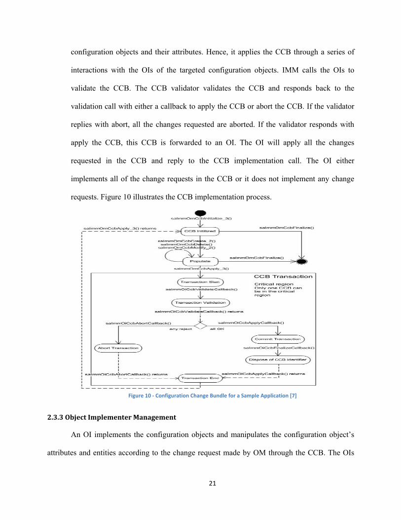
configuration objects and their attributes. Hence, it applies the CCB through a series of

interactions with the OIs of the targeted configuration objects. IMM calls the OIs to

validate the CCB. The CCB validator validates the CCB and responds back to the

validation call with either a callback to apply the CCB or abort the CCB. If the validator

replies with abort, all the changes requested are aborted. If the validator responds with

apply the CCB, this CCB is forwarded to an OI. The OI will apply all the changes

requested in the CCB and reply to the CCB implementation call. The OI either

implements all of the change requests in the CCB or it does not implement any change

requests. Figure 10 illustrates the CCB implementation process.

Figure 10 - Configuration Change Bundle for a Sample Application [7]

2.3.3 Object Implementer Management

An OI implements the configuration objects and manipulates the configuration object’s

attributes and entities according to the change request made by OM through the CCB. The OIs

21

are the applications that actually implement the configuration, hence they play three important

roles: the CCB applier, the CCB validator and the runtime owner roles [7].

As a runtime owner, an OI creates, deletes and performs administrative operations on

objects and updates the runtime information of objects and attributes in the IM. OM obtains the

runtime status of the AMF configuration from accessing the runtime attributes in the IM.

An OM creates configuration change requests through the CCB and submits it to IMM.

In order to assure consistency and coordination of configuration changes IMM needs to consult

the object validators and appliers. An OI that takes the role of the CCB validator, checks the type

and constraints of an attribute or an object as defined for the OI. IMM checks if the class and the

attributes are valid with respect to the IM. This type of validation is called the local validation.

After the local validation for all the changes requested, the OI carries out global validation,

which includes dependencies between the objects and attributes and the consistency of the IM

after the implementation of CCB. Finally OIs confirm that there are enough resources and all the

required OIs are present to carry out the CCB implementation. If IMM receives a confirmation

from all of the OIs that the CBB is valid, IMM will again call the OIs in the CCB applier role to

deploy the CCB. The appliers are aware of the changes in the validation phase itself; hence they

are prepared to implement the CCB. Once the CCB is applied the OI writes back in the IM to

inform the status of the CCB. If the CCB could not be applied all the CCB appliers are informed

that the transaction has been cancelled and should not be processed further.

• Object Implementer Registration

We have already seen the roles that OI plays in maintaining the configuration in the IM.

OI processes are the processes that have the best knowledge of the IM and of the changes

in the IM. If an application process wants to have the privileges of being notified of

22

configuration changes like the creation of new SIs, etc. It is possible for the process to

register itself as an OI of the object.

The process needs to first select an OI name and register with IMM. This will create a

link between the process and the OI name. The OI name is already set at the class level

and IMM automatically creates a link between the object and the OI name that is set for

the class. Hence all the objects of the same class will have the same OI. Thus, a process

that wants to act as an OI of any particular object has to register itself with the same name

as that of the object’s OI name. IMM informs all the processes that are registered as the

OI about any updates and administrative operations requested on the object.

2.4 Related Work

In this section we will review work of other researchers on availability and elasticity in

cloud computing and also cluster computing environments. Most of the related work in cloud

and cluster computing environments handle either elasticity or availability but not both

simultaneously. Moreover, some work are actually more about scalability than elasticity as

distinguished in [3].

OpenStack [11] is the most popular cloud controller and it consists of several related

projects among which the Heat [12] and Ceilometer [13] projects are of particular interest to us.

Heat [17] [18] claims to provide auto-scaling (i.e. elasticity) and HA features within OpenStack.

It can automatically increase or decrease the number of VMs according to workload changes

based on some policies defined in the configuration. It can also restart services in the case of

failures. Ceilometer [14] provides metering service and informs Heat when workload changes

occur. Heat provisions or de-provisions the resources using a rather straight forward policy such

as adding one VM if the CPU or memory utilization is greater than 50% and removing a VM if

23

the utilization falls below 10%. Heat also reacts to application failures by restarting the

appropriate resources. But this reaction may take up to a minute, which is significant when

considering HA in terms of the five 9’s. Moreover, Heat provides availability and elasticity at

virtual infrastructure levels only.

The work in [15] [16] [17] focuses on elastic resource provisioning in clusters. The main

goal of this work is to provision resources to service requests as they arrive in queue and release

the resources on completion. The solution presented in this work maintains a job queue and

elastically provisions resources in a cluster according to the size of the queue maintained. The

author in [15], designed an elastic site manager and define policies to achieve elastic

provisioning of resources which also manage sudden workload increases by reserving adequate

resources. Murphy et al. [16] dynamically increase and decrease virtual organization clusters in

terms of the number of VMs, when the number of jobs in the queue change. The goal of the work

in [17] is to dynamically increase and decrease resources on workload changes but the main

focus of the author is to assign relevant tasks to appropriate resources and priority is given to

load balancing rather than allocating resources to application services. The drawbacks of this

work are that the solutions presented in the work require the service requests to be maintained in

the queue which is an overhead and the authors of this work assume very specific design

architecture of the application. Furthermore, the solution presented in [15] [16] [17], only focus

on elastic provision of virtual infrastructure resources (like VMs).

The work in [19] [20] focuses on on-demand infrastructure resource provisioning. Zhang

et al [18] focuses on providing infrastructure resources on-demand by first trying to improve

resource utilization of the loaded application, and then allocating more resources if required.

Yang et al. [19] use a profile-based approach to capture the expert’s knowledge of just-in-time

24

scaling (i.e. elasticity) applications. Other researchers have proposed workload predictions for

more efficient elasticity handling [20].

In [21], the goal is to assure service scalability in service-oriented computing. The author

proposes two approaches to assure scalability: service replication and migration, to increase

resources allocated to a service. Thus, the work is more focused on scalability rather than

elasticity as distinguished in [3].

The work in [22] [23], mainly focus on dynamic scaling of web applications. The goal of

the author is to dynamically provision and de-provisions VMs according to the workload change.

They use load balancer to distribute web application loads across resources (VMs). In this work

they focus on the automatic scalability of virtual resources and dynamic distribution of web

services using a load balancer. The work does not handle availability and elasticity at an

application level.

In this sub-section, we presented literature work from different perspectives that can be

directly or indirectly related to our work. Most of the literature focusses either on availability or

elasticity but does not provide a solution for elasticity and availability together. Some solutions,

like OpenStack, provide a solution for elasticity and availability but at the virtual infrastructure

level only.

25

Chapter 3 - Elasticity in Availability Management Framework

In this chapter, we discuss the attributes in the AMF configuration that play a role in

elasticity management, the constraints applicable to them as well as their impact on load

distribution.

3.1 Elasticity Related Attributes in an AMF Configuration

An AMF configuration consists of the description of entities such as components, SUs,

SGs, SIs, CSIs with their respective types, nodes and their relations. These entities are described

in the AMF configuration with the help of objects and their attributes of the classes defined by

the AMF specification [4]. The attributes are either configuration (read-only or writable) or

runtime attributes [4]. The OMs (e.g. configuration designers, system administrators,

management applications, etc.) set the configuration attributes, while the runtime attributes are

set by AMF at runtime. AMF receives the changes in configuration attributes, evaluates the

system state and implements the configuration changes while maintaining service availability.

We can force AMF to change the SI-to-SU assignment by modifying the values of writable

configuration attributes and as a result re-distribute the workload generally within a given SG

and a cluster.

We illustrate with an example, the service side and service provider side attributes of the

AMF configuration, which can be modified to achieve elasticity in an AMF configuration.

Figure 11 shows, a highly available web application. An SG of the N-way-Active redundancy

model type protects the web application service hosted on four nodes. The SG consists of four

SUs, namely SU1, SU2, SU3 and SU4 hosted on four nodes. Each SU consists of two

26

components ‘http-server’ and ‘application server’ (AS) that collaborate closely to provide the

web application service. There are two SIs, SI1 and SI2 that define the web service workload.

Each SI consists of two CSIs, the http-CSI and the AS-CSI.

• saAmfSGAutoAdjust:SaBoolT = SA_TRUE

This attribute indicates to AMF that it must transfer back a SI assignment to the most

preferred SU in an SG whenever a highest-ranked SU is available in the SG. This attribute is

important to enable elasticity in AMF. It needs to be set to SA_TRUE if not set. In the

example of the web service application this attribute is set to SA_TRUE.

• saAmfSGNumPrefInserviceSUs = 4

This attribute denotes the number of SUs of the SG that are ready to accept a SI assignment.

The components of the in-service SUs have all the required software and services installed to

handle the SI assignments. In the example of web service application this attribute is set to

four. The attribute should not be set to more than the number of SUs actually configured in

the AMF configuration or set to less that the number of SUs required for SI assignments.

• saAmfSGNumPrefAssignedSUs = 3

This attribute denotes the number of SUs that AMF can use for assigning SIs. The

constraining attributes provide an upper bound and lower bound range within which the

value can be set for this attribute. The attribute value of ‘saAmfSGNumPrefInserviceSUs’

constrains the value of the attribute ‘saAmfSGNumPrefAssignedSUs’ by not allowing the

‘saAmfSGNumPrefAssignedSUs’ attribute value to be set to lower than ‘four’ in our example.

27

Figure 11 - Example of Web Service Application

• saAmfSGMaxActiveSIsperSU =2

This attribute specifies the maximum number of active SIs that can be simultaneously

assigned to a SU. The value of the attribute can be increased up to the value set for the

configuration attribute ‘saAmfCtDefNumMaxActiveCSIs’ [4]. This attribute of AMF defines

the maximum number of CSIs (of a particular service type) that the components of the SG

can handle simultaneously.

• saAmfSIPrefActiveAssignments

This attribute is only applicable to a SG with an N-way-Active redundancy model. It

specifies the number of SUs that need to be assigned to the SI. For the example,

‘SI1.saAmfSIPrefActiveAssignment=2’ and ‘SI2.saAmfSIPrefActiveAssignment=2’.The value

of this attribute must not be less than ‘two’ to maintain service availability.

In the example, if the workload of SI1 increases, we can increase the attribute value of

‘saAmfSGNumPrefAssignedSUs’ of the SG and the SI1’s attribute value of

‘saAmfSIPrefActiveAssignments’, which will force AMF to assign more SUs to SI1. If the

28

workload of SI1 decreases, we can decrease the SI1’s attribute value of

‘saAmfSIPrefActiveAssignments’, which will force AMF to free the SUs assigned to SI1. We can

change the AMF configuration attributes to force AMF to increase or decrease resources when

the workloads of services change.

The AMF configuration attributes from the service side and service provider side that can

be modified for elasticity are referred to as elasticity attributes in the rest of this thesis. When the

elasticity attributes are modified, AMF applies the changes in the system while maintaining HA.

To maintain HA of the services the AMF configuration needs to be valid throughout the

modifications. Therefore to apply valid changes to the AMF configuration all of the

dependencies among entities need to be checked and whether system will be able to provide and

protect the needed services after the elasticity attribute changes need to be determined. There are

various configuration attributes at various levels of the AMF configuration that constrain the

elasticity attributes. The AMF domain model [24] captures all of these constraints and expresses

it with the help of Object Constraint Language (OCL) [25]. Table 1 and Table 2 list all of the

elasticity attributes and the constraints on them.

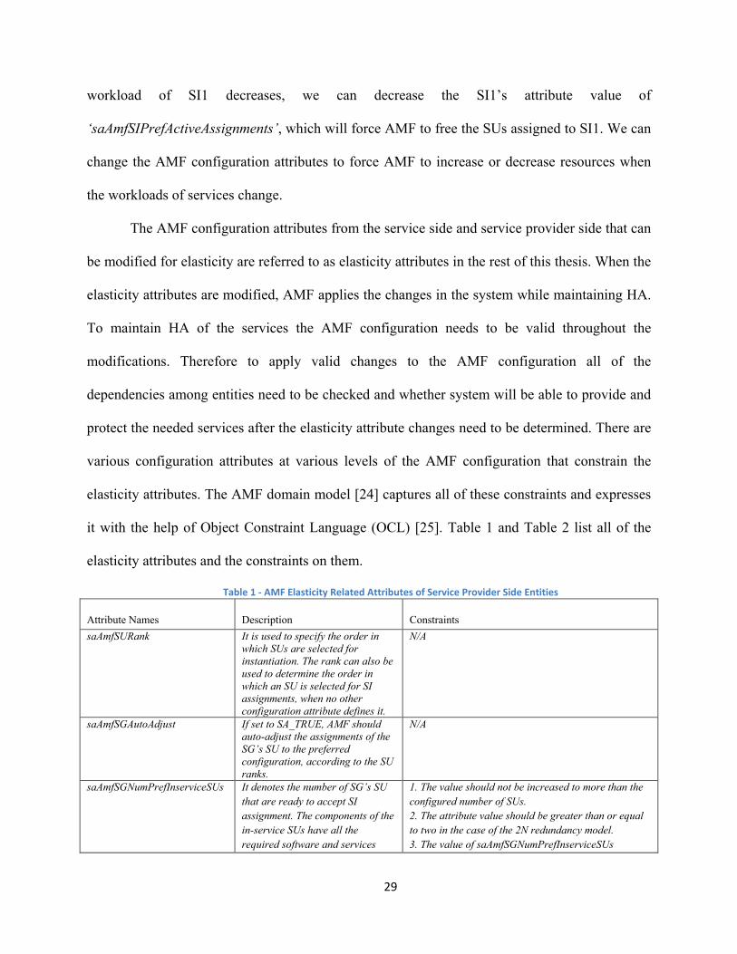
Table 1 - AMF Elasticity Related Attributes of Service Provider Side Entities Attribute Names

Description

Constraints saAmfSURank It is used to specify the order in

which SUs are selected for instantiation. The rank can also be used to determine the order in which an SU is selected for SI assignments, when no other configuration attribute defines it.

N/A

saAmfSGAutoAdjust If set to SA_TRUE, AMF should auto-adjust the assignments of the SG’s SU to the preferred configuration, according to the SU ranks.

N/A

saAmfSGNumPrefInserviceSUs It denotes the number of SG’s SU that are ready to accept SI assignment. The components of the in-service SUs have all the required software and services

1. The value should not be increased to more than the configured number of SUs. 2. The attribute value should be greater than or equal to two in the case of the 2N redundancy model. 3. The value of saAmfSGNumPrefInserviceSUs

29

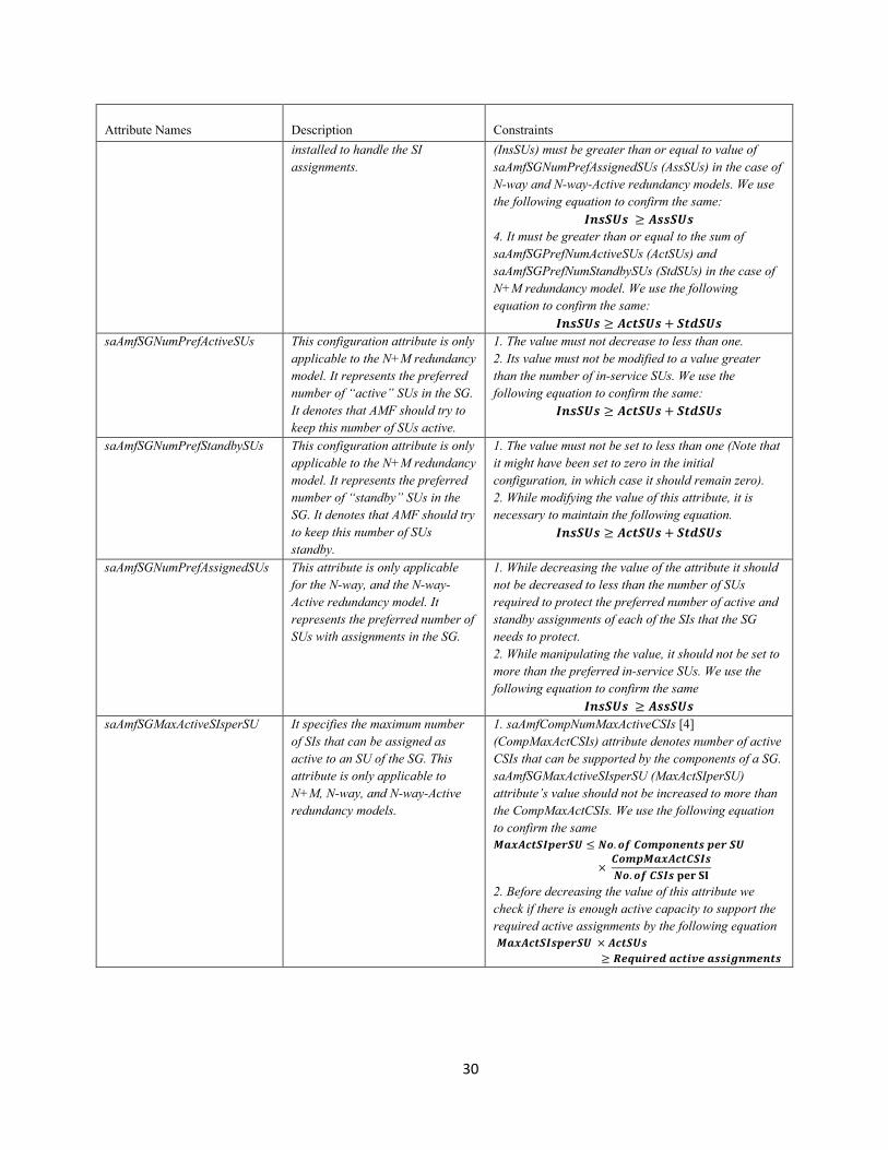
Attribute Names

Description

Constraints installed to handle the SI

assignments.

(InsSUs) must be greater than or equal to value of saAmfSGNumPrefAssignedSUs (AssSUs) in the case of N-way and N-way-Active redundancy models. We use the following equation to confirm the same:

𝑰𝒏𝒔𝑺𝑼𝒔 ≥ 𝑨𝒔𝒔𝑺𝑼𝒔 4. It must be greater than or equal to the sum of saAmfSGPrefNumActiveSUs (ActSUs) and saAmfSGPrefNumStandbySUs (StdSUs) in the case of N+M redundancy model. We use the following equation to confirm the same:

𝑰𝒏𝒔𝑺𝑼𝒔 ≥ 𝑨𝒄𝒕𝑺𝑼𝒔 + 𝑺𝒕𝒅𝑺𝑼𝒔 saAmfSGNumPrefActiveSUs This configuration attribute is only

applicable to the N+M redundancy model. It represents the preferred number of “active” SUs in the SG. It denotes that AMF should try to keep this number of SUs active.

1. The value must not decrease to less than one. 2. Its value must not be modified to a value greater than the number of in-service SUs. We use the following equation to confirm the same:

𝑰𝒏𝒔𝑺𝑼𝒔 ≥ 𝑨𝒄𝒕𝑺𝑼𝒔 + 𝑺𝒕𝒅𝑺𝑼𝒔

saAmfSGNumPrefStandbySUs This configuration attribute is only applicable to the N+M redundancy model. It represents the preferred number of “standby” SUs in the SG. It denotes that AMF should try to keep this number of SUs standby.

1. The value must not be set to less than one (Note that it might have been set to zero in the initial configuration, in which case it should remain zero). 2. While modifying the value of this attribute, it is necessary to maintain the following equation.

𝑰𝒏𝒔𝑺𝑼𝒔 ≥ 𝑨𝒄𝒕𝑺𝑼𝒔 + 𝑺𝒕𝒅𝑺𝑼𝒔

saAmfSGNumPrefAssignedSUs This attribute is only applicable for the N-way, and the N-way-Active redundancy model. It represents the preferred number of SUs with assignments in the SG.

1. While decreasing the value of the attribute it should not be decreased to less than the number of SUs required to protect the preferred number of active and standby assignments of each of the SIs that the SG needs to protect. 2. While manipulating the value, it should not be set to more than the preferred in-service SUs. We use the following equation to confirm the same

𝑰𝒏𝒔𝑺𝑼𝒔 ≥ 𝑨𝒔𝒔𝑺𝑼𝒔 saAmfSGMaxActiveSIsperSU It specifies the maximum number

of SIs that can be assigned as active to an SU of the SG. This attribute is only applicable to N+M, N-way, and N-way-Active redundancy models.

1. saAmfCompNumMaxActiveCSIs [4] (CompMaxActCSIs) attribute denotes number of active CSIs that can be supported by the components of a SG. saAmfSGMaxActiveSIsperSU (MaxActSIperSU) attribute’s value should not be increased to more than the CompMaxActCSIs. We use the following equation to confirm the same 𝑴𝒂𝒙𝑨𝒄𝒕𝑺𝑰𝒑𝒆𝒓𝑺𝑼 ≤ 𝑵𝒐.𝒐𝒇 𝑪𝒐𝒎𝒑𝒐𝒏𝒆𝒏𝒕𝒔 𝒑𝒆𝒓 𝑺𝑼

× 𝑪𝒐𝒎𝒑𝑴𝒂𝒙𝑨𝒄𝒕𝑪𝑺𝑰𝒔𝑵𝒐.𝒐𝒇 𝑪𝑺𝑰𝒔 𝐩𝐞𝐫 𝐒𝐈

2. Before decreasing the value of this attribute we check if there is enough active capacity to support the required active assignments by the following equation 𝑴𝒂𝒙𝑨𝒄𝒕𝑺𝑰𝒔𝒑𝒆𝒓𝑺𝑼 × 𝑨𝒄𝒕𝑺𝑼𝒔

≥ 𝑹𝒆𝒒𝒖𝒊𝒓𝒆𝒅 𝒂𝒄𝒕𝒊𝒗𝒆 𝒂𝒔𝒔𝒊𝒈𝒏𝒎𝒆𝒏𝒕𝒔

30

Attribute Names

Description

Constraints saAmfSGMaxStandbySIsperSU This attribute specifies the

maximum number of SIs that can be assigned as standby to a SU of the SG. This attribute is only applicable to N+M and N-way redundancy models

1. saAmfCompNumMaxStandbyCSIs [4] (CompMaxStdCSIs) attribute denotes the number of standby CSIs that can be supported by the components of a SG. saAmfSGMaxStandbySIsperSU (MaxStdSIperSU) attribute’s value should not be increased to more than the CompMaxStdCSIs. We use the following equation to confirm the same

𝑴𝒂𝒙𝑺𝒕𝒅𝑺𝑰𝒑𝒆𝒓𝑺𝑼 ≤ 𝑵𝒐.𝒐𝒇 𝑪𝒐𝒎𝒑𝒐𝒏𝒆𝒏𝒕𝒔 𝒑𝒆𝒓 𝑺𝑼𝒔

× 𝑪𝒐𝒎𝒑𝑴𝒂𝒙𝑺𝒕𝒅𝑪𝑺𝑰𝒔𝑵𝒐.𝒐𝒇 𝑪𝑺𝑰𝒔 𝐩𝐞𝐫 𝐒𝐈

2. Before decreasing the value of this attribute we check if there is enough standby capacity to support required standby assignments by using the following equation

𝑴𝒂𝒙𝑺𝒕𝒅𝑺𝑰𝒑𝒆𝒓𝑺𝑼 × 𝑺𝒕𝒅𝑺𝑼𝒔≥ 𝑹𝒆𝒒𝒖𝒊𝒓𝒆𝒅 𝒔𝒕𝒂𝒏𝒅𝒃𝒚 𝒂𝒔𝒔𝒊𝒈𝒏𝒎𝒆𝒏𝒕𝒔

saAmfNodeCapacity This attribute specifies the capacity of the node to configure SUs and SIs

N/A

The service side attributes are listed in Table 2.

Table 2- AMF elasticity related attributes of service side entities Attribute Names

Description

Constraints saAmfSIRank SI rank is used to specify the

order in which SIs are selected for the assignment.

N/A

saAmfSIPrefActiveAssignments This attribute represents the preferred number of active assignments per SI in the N-way-Active redundancy model. It is not applicable for the other redundancy models.

1. The attribute value should not be decreased to less than two. 2. saAmfSIPrefActiveAssignments (SIAssgmnts) attribute value may be increased, only if the SI needing capacity is not assigned yet to all the SUs in the SG. We check the same by the following equation:

𝑺𝑰𝑨𝒔𝒔𝒈𝒎𝒏𝒕𝒔 ≤ 𝑨𝒔𝒔𝑺𝑼𝒔 And if the SG has enough capacity. We confirm the same by the following equation. 𝑺𝑰𝑨𝒔𝒔𝒈𝒎𝒏𝒕𝒔 ≤ 𝑴𝒂𝒙𝑨𝒄𝒕𝑺𝑰𝒑𝒆𝒓𝑺𝑼 × 𝑨𝒔𝒔𝑺𝑼𝒔

saAmfSIPrefStandbyAssignments This attribute represents the preferred number of standby assignments per SI in the N-way redundancy model. It is not applicable for the other redundancy models.

1. The attribute value should not be decreased to less than two.

saAmfSIActiveWeight SI weight for active assignments of this SI.

N/A

saAmfSIStandbyWeight SI weight for standby assignments of this SI.

N/A

saAmfSIRankedSU This is used to specify the ranked list of SUs per SI; It is applicable for the SGs with N-way and N-way-Active redundancy models.

N/A

31

The aforementioned attributes are writable configuration attributes. We can manipulate

the values of these attributes to force AMF to change the SI-to-SU assignments, which will re-

distribute the workload within a given SG or cluster in general. This, in turn, increases and

decreases resources to different SIs representing workloads in the system. Therefore, we can

achieve our objective of managing elasticity within AMF by selecting an appropriate

combination of the AMF configuration modifications that change the resources depending on the

workload changes.

3.2 Types of workload changes in an AMF Configuration

Now that we have determined the elasticity attributes and their constraints, we will define

the two types of workload changes in an AMF configuration. The two types of workload changes

characterize the potential changes in the workload of an AMF configuration. In an AMF

configuration a workload is represented by SIs that consists of CSIs. The workload may increase

or decrease due to change in the user’s requests. This change in workload triggers elasticity

action; hence it is mandatory to characterize the potential changes in workload. The section

describes the two types of workload changes: Single-SI and Multiple-SI type workload changes.

3.2.1 Single-SI Type workload changes

When the workload change maps to the single SI pre-existing in the AMF configuration,

we define it as a Single-SI change. For example, if the SI is defined as a Uniform Resource

Locator (URL) through which users access a given service, any increase of user requests will still

be represented in the AMF configuration by the same SI. We can say that the workload imposed

by the single SI has increased as shown in Figure 12(A). Similarly, any decrease of user requests

will still be represented in the AMF configuration by the same SI, so we can say that the

32

workload of this single SI has decreased as shown in Figure 12(B). We assume that changes in

the workload associated with a single SI are detected by a workload monitor.

Figure 12 - Example for Single-SI type workload changes

3.2.2 Multiple-SI type workload changes

When the change in the workload manifests as an increase or a decrease in the number of

SIs in the AMF configuration, we define it as Multiple-SI change. For example, if an SI is

defined as the VLC media player [26], any increase in the number of requests for the VLC will

map to a new SI in the AMF configuration as shown in Figure 13(A). Also, any decrease in VLC

requests will result in decreasing the number of SIs as shown in Figure 13(B). Multiple-SI type

workload change is associated to a configuration change performed through IMM.

33

Figure 13 - Example of Multiple-SI type workload changes

3.3 Summary

In this chapter we determined the AMF configuration attributes related to elasticity and

the attributes constraining them. Our goal is to enable elasticity and availability in the AMF

configuration. We enable elasticity in the AMF configuration by manipulating the AMF

configuration attributes related to elasticity. To guarantee availability we need to check the

constraints before modifying the AMF configuration attributes. To characterize the potential

workload changes in an AMF configuration, we also defined ‘Single-SI’ and ‘Multiple-SI’ type

of workload changes. The Single-SI type of workload changes in an AMF configuration are

detected by the workload monitor. The Multiple-SI type of workload changes are declared by the

IMM service. We will enable elasticity in the AMF configuration in the case of Single-SI or

Multiple-SI type of workload changes.

34

Chapter 4 - Overall Architecture and Elasticity Engine

In this chapter, we present our solution for managing elasticity and availability with the

SA Forum middleware. We elaborate on EE architecture and its behavior through the elasticity

strategies.

4.1 Overall architecture for HA and elasticity management

AMF is responsible for maintaining the availability of the system. AMF receives the

configuration changes from IMM and acts accordingly [4]. A monitor(s) is required to detect the

application workload changes and inform the EE about any significant change (e.g. exceeding a

given threshold). The workload changes detected by the monitor are associated with the same SI,

i.e. they are of type ‘Single-SI’ workload change. The workload in the AMF configuration may

also change due to an increase or decrease in the number of SIs i.e. Multiple-SI type workload

change. The number of SIs can be changed by modifying the AMF configuration through the

IMM service. In this case, the EE expects a notification from IMM.

When the EE receives a signal that the workload has increased or decreased from the

monitor or IMM, it reads the configuration in the IM using the IMM service to calculate the

configuration changes necessary to adjust the system. It then writes the CCBs into IMM, and

AMF in turn receives these changes (i.e. CCBs) from IMM and implements them by rearranging

the SI-to-SU assignments as necessary. Once AMF implements the CCB, AMF updates the

runtime attributes of the configuration objects. The EE also informs the system manager or cloud

manager to increase the number of nodes in the cluster and install required software on them to

35

keep the system ready for further workload changes. Figure 18 shows the overall architecture for

HA and elasticity management with AMF.

Figure 14 - Overall Architecture for HA and Elasticity Management with AMF

4.2 The Elasticity Engine Architecture

The EE is composed of the “Elasticity Controller”, the “Redundancy Model (RM)

Adjustors” and the “Buffer Manager” as shown in Figure 15. At a high level of abstraction the

operation of the EE consists of the following steps:

1. The EE receives the indication that the workload has changed in two ways:

a. The workload monitor(s) monitors the actual workload associated with an SI and signals

the need of an adjustment if there is a significant change in the workload (for example, an

increase or decrease in the incoming traffic exceeds some threshold).

b. The workload in the AMF configuration may also change due to the addition or removal

of services, that is, in the case of an increase or decrease in the number of SIs in the AMF

configuration, the EE receives the information about these changes from IMM.

36

2. After receiving the workload change signals, the EE Controller reads the AMF configuration

in the IM to determine the SG protecting the SI that has changed in workload. Depending on

the SG’s redundancy model the EE Controller calls the RM Adjustor.

3. The RM Adjustor reads the AMF configuration attributes of the SG in the IM using IMM and

calculates the configuration changes (i.e. CCBs) required to adjust the SG’s configuration to

the received workload changes. The configuration changes accommodate any additional

workload or release any resources in excess while maintaining availability. The RM Adjustor

creates and applies CCBs according to the various strategies defined in the next section.

4. To speed up future adjustments some nodes may be reserved for the SG, therefore the RM

Adjustor calls the Buffer Manager to reserve nodes or free up allocated nodes through

additional CCBs. Depending on the outcome of the adjustments the EE Controller may take

one or more of the following actions:

If the adjustments of the given SG are insufficient: The EE Controller will do similar

configuration adjustments of other SGs which have similar redundancy model and are

sharing nodes with the SG requiring capacity.

Towards the administrator or cloud manager: The EE Controller will inform to add or

remove nodes in the cluster, if the cluster size is insufficient or if some nodes are

freed up, and/or

Towards the administrator or software management: The EE Controller will inform

the installation of required software on additional nodes within the cluster if new

nodes are needed to be able to cope with the workload increase.

37

Figure 15 - The Architecture of Elasticity Engine

The sequence diagram in Figure 16 shows the EE’s sequence of actions to handle

workload changes.

38

Figure 16 – Elasticity Engine’s Sequence Diagram

4.3 Elasticity Engine Strategies

The EE handles workload changes depending on the redundancy model of the SG

protecting the SI in the AMF configuration. It first tries to adjust the workload changes at the SG

level by adjusting the configuration of the SG protecting the affected SI. If the SG level

39

adjustments is not possible it tries to adjust workload changes at the cluster level where it tries to

adjust the configuration for other SGs and SIs in the cluster sharing nodes with the SG protecting

the affected SI. The EE’s RM Adjustors handle the workload changes. Each of the RM Adjustor

uses a combination of the following strategies. The combination of the strategies depends on the

redundancy model type of the SG and the execution state of the system while applying the

strategies.

4.3.1 Workload increase

If the monitor reports an increase in the workload of an SI (i.e. Single-SI type workload

changes), the EE will try to increase the capacity assigned to the SI. If the workload increase is

due to a new SI (i.e. Multiple-SI type workload changes), the EE checks if the new SI is not

already assigned before increasing the capacity in the SG for the new SI. However, the strategies

used to handle the workload increase are the same. We define three main strategies to handle the

workload increase:

Spreading the SI workload

In this strategy we handle a service workload increase by spreading it over more nodes.

The EE uses this strategy when an SG protecting the SI is an ‘N-way-Active’

redundancy model. The EE will handle the increase of the workload of an SI by

increasing the number of assignments of the SI in the SG protecting it. Thus, the

workload increase of the SI is handled by spreading it across more SUs. Figure 17 shows

the workload of the SI before (A) and after (B) the adjustment. The orange portion

indicates the capacity used by SIs protected by SG1, the green portion denotes the

capacity used by SI1 and the blue portion indicates the capacity used by SI2 protected by

SG2. The light blue portion indicates the increase in workload (A) of SI1. The SG2 is of

40

the N-way-Active redundancy model and its SUs are configured on all of the nodes in

the figure. According to the strategy the assignment of SI2 protected by SG2 is

incremented from two to three, thus, the SI2’s workload is distributed on an additional

Node3 and the workload increase is handled.

Figure 17 - Spreading the SI workload

Distributing the SIs over more SUs

In this strategy we handle workload increase by distributing the services configured on

the loaded node over more number of nodes. At the SG level the EE may handle the

increase of the workload of an SI by distributing the SIs to more SUs within the SG,

therefore giving more capacity to each SI including the one experiencing the increase.

This strategy cannot be applied to the 2N and the No-Redundancy redundancy models.

In Figure 18, the capacity used by SIs protected by SG1 is indicated in orange. The green

indicates the portion used by SI1, the blue indicates the portion used by SI2 and the red

portion indicates the capacity used by the SI3 of SG2. The SUs of SG2 are configured on

all the nodes. In Figure 18(A) the light blue portion indicates an increase in workload of

SI1 protected by SG2. According to this strategy EE decreases the number of SIs that

can be assigned to a SU from two to one and the number of assigned (or active) SUs

from two to three. This will force AMF to move SI2 protected by SG2 to Node3.

41

Figure 18 - Distributing the SIs over more SUs

Prioritizing the SU on the least loaded node

In this strategy we handle the service workload increase by re-assigning the services

from loaded node to least loaded node. The EE may handle an increase in the workload

of an SI by swapping the rank of the SU currently active for the SI with rank of the SU

on the least loaded node. This will cause AMF to move the SIs of the currently active

SU to a node having more capacity. The EE uses this strategy when a SG protecting the

SI experiencing workload increase, is of a 2N or No-Redundancy redundancy model.

We can apply the strategy to other redundancy models as well however it may contradict

other considerations guiding the ranks, such as balancing SIs within SG. In Figure

19(A), Node1 is used to serve SIs protected by SG1 indicated by orange. Capacity used

by SI1 and SI2 protected by SG2 is indicated by green and blue colors respectively. The

light blue portion in Figure 19(A) indicates a workload increase in SG2. Since the SUs

of SG1 and SG2 are configured on all of the nodes, the SG2’s SU on Node3 can be

prioritized. This will force AMF to move the assignments to Node3 as shown in Figure

19(B).

42

Figure 19 - Prioritizing the SU on the least loaded node

4.3.2 Workload decrease

The EE handles a workload decrease by freeing SUs of the SG, which indirectly may free

the nodes that host these SUs. The EE will first try to free up some capacities of the SG

protecting the SI and may then try at the cluster level with other SGs. The EE applies workload

decrease strategies according to the redundancy model type of the SG that protects the SI and the

current execution state of the system. These strategies are opposite to the strategies that handle

workload increase.

Merging the SI workload In this strategy we handle the service workload decrease by

spreading it over less nodes. At the SG level the EE may handle the decrease of the

workload of an SI by decreasing the number of SI assignments and therefore distributing

the SI’s workload to smaller number of SUs within the SG. The EE uses this strategy

when an SG protecting the SI is of an N-way-Active redundancy model. Figure 20 shows

the workload of the SI before (A) and after (B) the adjustment. The orange portion

indicates the capacity used by SIs protected by SG1, the green portion denotes the

capacity used by SI1 and the blue portion indicates the capacity used by SI2 protected by

SG2. The light blue portion indicates the decrease in workload of SI2 (A). The SG2 is of

43

an N-way-Active redundancy model type and its SUs are configured on all of the nodes

in the figure. According to the strategy the assignments of SI2 protected by SG2 is

decremented from three to two, thus its load is distributed on only two nodes.

Figure 20 - Merging the SI workload

Re-grouping the SIs to less SUs of the SG

In this strategy we handle the workload decrease by distributing the services over less

nodes. In other words, at the SG level the EE may handle a decrease in workload of an

SI by redistributing the SIs to lower number of SUs within the SG, therefore reducing

the capacity provided to the SIs including the one experiencing the decrease.

Accordingly, each SI protected by the SG should allow for such a decrease. This strategy

cannot be applied to the 2N and the No-Redundancy redundancy models. In Figure 21,

the orange portion indicates the capacity used by SIs of SG1. The blue portion indicates

the capacity used by SI1, the green portion indicates the capacity used by SI2 and the red

portion indicates the capacity used by SI3 protected by SG2. The light blue portion

indicates the workload decrease in SI1 of SG2. According to this strategy the EE

increases the number of SIs that can be assigned to a SU from one to two and reduces the

number of assigned (or active) SUs from three to two This will force AMF to move SI2

to Node1 as shown in Figure 21(B).

44

Figure 21 - Re-grouping the SIs to less SUs of the SG

Prioritizing the nodes that serve other SIs

In this strategy we handle the workload decrease by re-assigning the services to another

node handling some services in order to free the current node. The EE may handle a

decrease in the workload of an SI by swapping the rank of a SU currently active for the

SI with the rank of a SU on a node that has other assignments as well. As a result AMF

will move the assignments of the current active SU to the already loaded node as shown

in Figure 22. The EE uses this strategy primarily when an SG protecting the SI

experiencing a workload decrease is of a 2N or No-Redundancy redundancy model. In

Figure 22, the orange portion indicates the capacity used by SIs protected by SG1. The

blue portion indicates the capacity used by SI1 and green indicates the portion of

capacity used by SI2. The SI1 and SI2 are protected by SG2. The light blue portion

indicates the workload decrease of SI1 indicated in Figure 22(A). Since SUs of SG2 are

configured on all the nodes in the figure, the SU on Node1 can be prioritized according

to this strategy. This will force AMF to move the assignments of SI1 and SI2 to Node1

as shown in Figure 21(B).

45

Figure 22 - Prioritizing the nodes that serve other SIs

4.3.3 Buffer management

In the AMF configuration, only a subset of the configured SUs in an SG are in-service

SUs and AMF can only use the number of assigned SUs among the in-service SUs for SI

assignments. In-service SUs are those instantiated and ready to serve the SI assignments but not

necessarily assigned yet. The un-instantiated spare SUs in an SG are those that are configured in

the SG but not in service; however they can easily be instantiated. To increase the resources to

handle a workload increase, the EE increases the number of assigned SUs (those on which AMF

can distribute the SI assignments) and decreases the number of assigned SUs, if the workload

decreases. The EE can use these different subsets to prepare AMF for sudden workload increases

by reserving additional SUs at different levels as buffers. In other words, in this strategy we

reserve enough nodes in the cluster to keep the system ready to handle sudden workload changes.

These SUs are reserved in two types of Buffers: The ‘in-service-SU-buffer’ and the ‘un-

instantiated-SU-buffer’.

The ‘in-service-SU-buffer’ is the number of instantiated SUs ready for service but not

used for assignments yet. They may be added quickly to the pool of SUs used for assignments or

in the case of failure they replace a failed SU. The in-service-SU-buffer is the difference between

46

the number of in-service SUs and the number of assigned SUs (or the sum of active and standby

SUs) of an SG. These SUs may use some resources, as they may be instantiated.

The ‘un-instantiated-SU-buffer’ indicates that the SUs in the buffer are ready for

instantiation as they have all the necessary software installed. These SUs have been configured

in the SG but are not instantiated by AMF; hence they do not consume resources. The un-

instantiated-SU-buffer is the difference between the number of configured SUs and in-service

SUs of an SG.

The size of the in-service-SU-buffer and the un-instantiated-SU-buffer is configurable.

The number of SUs in an in-service-SU-buffer is set according to the time required for the

adjustments, the time required to handle the increase in workload by an SG and the time required

to instantiate a SU in the un-instantiated-SU-buffer. The number of SUs in the un-instantiated-

SU-buffer is set according to the time required to install the required software on a node and/or

increase the number of nodes in the cluster. When the EE changes the number of assigned SUs

(or the number of active and standby SUs) it also adjusts the other configuration attributes in an

SG to maintain the required number of SUs in the buffers.

Reservation of Resources

When the EE increases the number of assigned SUs of the SG, it also prepares for any

sudden workload increase by bringing into service some additional SUs to maintain the

size of in-service-SU-buffer. The EE can increase the number of in-service SUs only if

there are additional SUs configured in an SG. Therefore the EE also ensures that there

are some un-instantiated spare SUs configured in the SG to maintain the un-instantiated-

SU-buffer. Otherwise the EE tries to configure new SUs. This is possible if there are

nodes in the node group configured for the SG that are not hosting any SUs and have the

47

required software installed on them. Otherwise, the EE signals to the system

administrator or cloud manager to configure new nodes with the required software

installed on them.

Freeing Reserved Resources

In the case of a decrease in the workload, the EE tries to free resources by decreasing the

number of assigned SUs. If this is successful the EE also decreases the number of in-

service SUs while maintaining the in-service-SU-buffer. It may also decrease the number

of configured SUs if the un-instantiated-SU-buffer is maintained. However this is not

absolutely necessary.

Figure 23 indicates the buffer management action of the EE. In Figure 23(A), the SUs of

the SG can be hosted on all of the seven nodes, amongst which only six nodes have the

SUs configured. The in-service SUs are five amongst which dark blue colored nodes

host the assigned SUs while the light blue colored nodes host the spare in-service

instantiated SUs. We take the size of the in-service-SU-buffer to be two SUs and the un-

instantiated-SU-Buffer to be one SU. In Figure 23(B), the EE’s action of resource

reservation is indicated. When the number of assigned SUs hosted on the nodes (dark

blue colored nodes) increase, the EE calculates the difference between the assigned SU

and the in-service SUs and increases the number of in-service units to six. Consequently,

it also configures a new SU on Node7. Figure 24(C) indicates the EE’s action to free the

reserved resources. When the number of assigned SUs hosted on the nodes (dark blue

colored nodes) decrease, the EE calculates the difference between the assigned SUs and

in-service SUs and decrease the in-service SUs to five.

48

Figure 23 - Buffer Manager

4.3.4 Cluster Level Adjustments

The services configured on the nodes in the cluster share resources. Hence, if we cannot

handle the workload change of a service within the group of nodes it is hosted, we may handle its

workload change by adjusting the workload of other services in the cluster. This adjustment will

result in the same effect for the service experiencing workload changes because the services are

hosted on the same nodes and share the node resources.

If the EE action for the configuration adjustment is unsuccessful at the SG level the EE

tries to adjust other SGs in the cluster. For this purpose the EE looks for similar SG sharing

resources with the one experiencing the workload change. If there is such an SG, the EE initiates

the same adjustment for an SI protected by this SG. The SI is also selected based on similarities.

This adjustment indirectly will result in the same effect for the original SG because the two SGs

are hosted on the same node and share the node resources. Hence either of the SGs can take the

node resources or release them.

49

Figure 24 shows two SGs of 2N redundancy models. Assuming that SG2 is configured

only on two nodes (Node1 and Node2) and SG1 is configured on all three nodes (Node1, Node2

and Node3). The orange portion indicates the capacity used by SIs protected by SG1 and the blue

portion indicates the capacity used by SIs protected by SG2. The light blue portion indicates the

increase in workload of SG2. In such a scenario, the EE cannot adjust at the SG level as shown

in Figure 24(A). It uses the cluster level adjustment to handle workload changes. The EE

prioritizes the SG1’s SU on Node3 forcing AMF to move the assignment of SI protected by SG1

to Node3.

Figure 24 - Cluster Level Adjustments

4.4 Elasticity Engine Algorithms

This section covers the detailed algorithms for the strategies discussed in the previous

section.

4.4.1 Workload increase algorithms

The EE applies the combination of the strategies to handle workload increases depending

on the redundancy model type of an SG and the current execution state of the system. The

redundancy model type of an SG determines the configuration attributes that the EE can adjust to

50

handle workload changes. Typically, these algorithms define the step by step procedure with the

configuration attributes that the EE’s RM Adjustor follows to handle workload changes.

• Spreading the SI workload

This algorithm defines the steps followed by the EE’s RM Adjustor to handle workload

increase of an SI protected by a SG of an N-way-Active redundancy model type (see Figure

25).

1. The RM Adjustor initializes two variables: ‘SI1’ with the name of the SI whose

workload has increased and ‘SG1’ with the name of the SG protecting this SI.

2. The EE’s RM Adjustor checks if the preferred number of active assignments attribute of

SI1 (saAmfSIPrefActiveAssignments) is less than the number of preferred assigned SUs

of SG1 (saAmfSGNumPrefAssignedSUs).

3. If the preferred number of active assignments of SI1 is less than the number of preferred

assigned SUs of SG1, the RM Adjustor checks if there is enough capacity configured in

SG1 to handle a new assignment of SI1.

a. If there is capacity, the RM Adjustor increases the preferred number of active

assignments of SI1. This will force AMF to assign SI1 to one more SU i.e. the

workload represented by SI1 spreads to more SUs.

b. If there is no capacity configured, the RM Adjustor checks if it can be configured

based on the capabilities of the components of the SUs. If so, it increases the number

of assignments each SU can take on and returns to Step 3 otherwise it follows with

Step 4.

4. If preferred number of active assignments of SI1 and the number of preferred assigned

SUs of SG1 are equal, that is, SI1 is already assigned to each assigned SU in SG1 then

51

the RM Adjustor tries to increase the number of preferred assigned SUs if there are spare

in-service SUs.

5. If the RM Adjustor has increased the number of preferred assigned SUs in SG1

(saAmfSGNumPrefAssignedSUs) it calls the Buffer Manager to reserve resources for

further workload increases and returns to Step 2.

6. If there are no in-service SUs i.e. SG1 is using all the nodes on which it can be hosted,

the RM Adjustor reports to the Elasticity Controller that it was not successful and the

adjustments need to be tried at the cluster level.

Start

SI1= SI requiring capacitySG1= SG protecting the SI1

SI1.saAmfSIPrefActiveAssignments < SG1.saAmfSGNumPrefAssignedSUs

SI1.saAmfSIPrefActiveAssignments < SG1.saAmfSGNumPrefAssignedSUs

>= sum(SI.saAmfSIPrefActiveAssignments)+1

Yes

IncreaseSI1.saAmfSIPrefActiveAssignments by 1

Yes

Inform Elasticity Controller that adjustment is successful

Stop

Component Capability Mode > SG1.saAmfSGMaxActiveSIsperSUNo

Increase SG1.saAmfSGMaxActiveSIsperSU by 1

Yes

SG1.saAmfSGNumPrefInserviceSUs > SG1.saAmfSGNumPrefAssignedSUsNo

NoElasticity on other SGs in the

cluster

No

Stop

Increase SG1.saAmfSGNumPrefAssignedSUs by 1

Yes

Call to Buffer Manager

Figure 25 - Flow-chart: Spreading the SI’s workload (N-way-Active Redundancy Model)

• Distributing the SIs over more SUs of SG

The EE follows the procedure defined in the following algorithm to handle workload

increases in the N-way-Active, the N+M and the N-way redundancy models (see Figure 26).

1. The EE’s RM Adjustor initializes five variables:

‘SI1’ with the name of the SI whose workload has increased,

‘SU1’ with the name of the SU currently assigned active for the SI1,

52

‘SG1’ with the name of the SG protecting this SI1,

‘ActiveSUs’ pointing to the preferred number of active SUs if SG1 is of N+M

redundancy model and to the preferred number of assigned SUs if SG1 is of the N-way

redundancy model, and

‘StandbySUs’ pointing to the preferred number of standby SUs if SG1 is of N+M

redundancy model and to the preferred number of assigned SUs if SG1 is of a N-way

redundancy model.

2. The RM Adjustor checks if it can decrease the maximum number of active assignments

on the SUs of SG1 (saAmfSGMaxActiveSIsperSU) without losing any SI assignments. If

yes, it tries to do so until the number of current active assignments assigned to SU1

decreases. If it is successful it proceeds to Step 5 to handle the standby side in a similar

manner.

3. If the RM Adjustor cannot decrease the maximum number of active assignments per SU

without losing SI assignments, it will then check to increase the SG1’s capacity by

increasing the value of the attribute ActiveSUs points to.

4. If the RM Adjustor is successful in increasing the number of active SUs, it invokes the

Buffer Manager and then returns to Step 2. Otherwise it reports to the Elasticity

Controller that the adjustments need to be made at the cluster level.

5. The RM Adjustor reinitializes ‘SU1’ with the name of the SU currently assigned standby

for SI1 if the SG1 is of an N+M redundancy model and the highest ranking SU if SG1 is

of the N-way redundancy model.

6. It checks if it can decrease the maximum number of standby assignments on the SUs of

SG1 (saAmfSGMaxStandbySIsperSU) without losing any SI assignments. If yes, it tries

53

to do so until the number of current standby assignments assigned to SU1 decreases. If

successful it reports to the Elasticity Controller about the success of the adjustments.

7. If the RM Adjustor cannot decrease the maximum number of standby assignments per

SU without losing an assignment, it will then try to increase the SG1’s standby capacity

by increasing the value of the attribute StandbySUs points to.

8. If the RM Adjustor is successful in increasing the number of standby SUs it invokes the

Buffer Manager and then returns to Step 6 otherwise it reports to the Elasticity

Controller that further adjustments are needed at the cluster level.

54

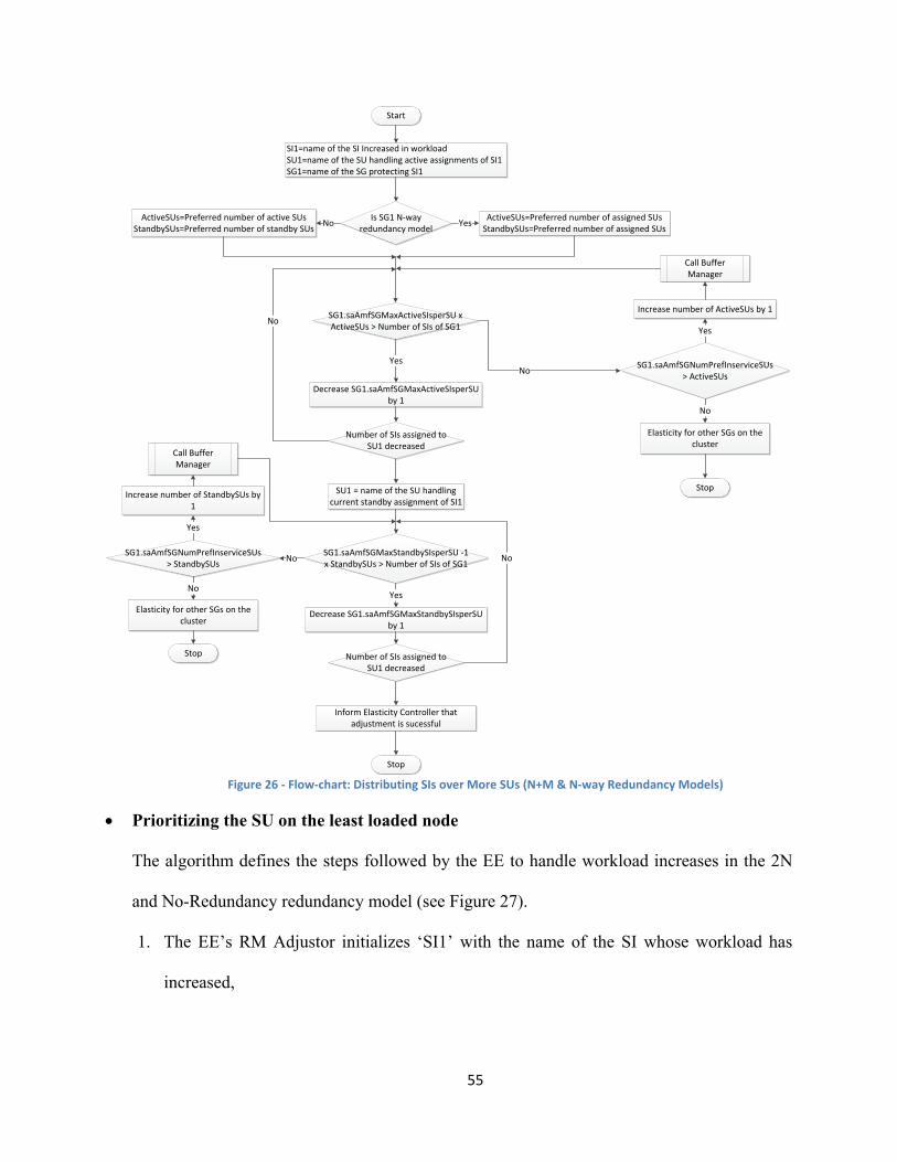
Start

SI1=name of the SI Increased in workloadSU1=name of the SU handling active assignments of SI1SG1=name of the SG protecting SI1

Is SG1 N-way redundancy model

ActiveSUs=Preferred number of assigned SUsStandbySUs=Preferred number of assigned SUsYesActiveSUs=Preferred number of active SUs

StandbySUs=Preferred number of standby SUs No

SG1.saAmfSGMaxActiveSIsperSU x ActiveSUs > Number of SIs of SG1

Decrease SG1.saAmfSGMaxActiveSIsperSU by 1

Yes

Number of SIs assigned to SU1 decreased

No

SG1.saAmfSGNumPrefInserviceSUs > ActiveSUsNo

Elasticity for other SGs on the cluster

No

Stop

Increase number of ActiveSUs by 1

Yes

Call Buffer Manager

SU1 = name of the SU handling current standby assignment of SI1

SG1.saAmfSGMaxStandbySIsperSU -1 x StandbySUs > Number of SIs of SG1

Decrease SG1.saAmfSGMaxStandbySIsperSU by 1

Yes

SG1.saAmfSGNumPrefInserviceSUs > StandbySUs No

Increase number of StandbySUs by 1

Yes

Call Buffer Manager

Elasticity for other SGs on the cluster

No

Stop Number of SIs assigned to SU1 decreased

No

Inform Elasticity Controller that adjustment is sucessful

Stop Figure 26 - Flow-chart: Distributing SIs over More SUs (N+M & N-way Redundancy Models)

• Prioritizing the SU on the least loaded node

The algorithm defines the steps followed by the EE to handle workload increases in the 2N

and No-Redundancy redundancy model (see Figure 27).

1. The EE’s RM Adjustor initializes ‘SI1’ with the name of the SI whose workload has

increased,

55

‘SU1’ with the name of the SU currently assigned active for the SI,

‘SG1’ with the name of the SG protecting this SI.

2. It finds the node hosting the SU1 and initializes ‘ActiveFinal’ with the sum of active

assignments handled by each SU hosted on the node and ‘StandbyFinal’ with the sum of

standby assignments handled by each SU hosted on the node.

3. It finds all the in-service SUs of SG1 and initializes an array ‘node1’ with the names of

nodes hosting them.

56

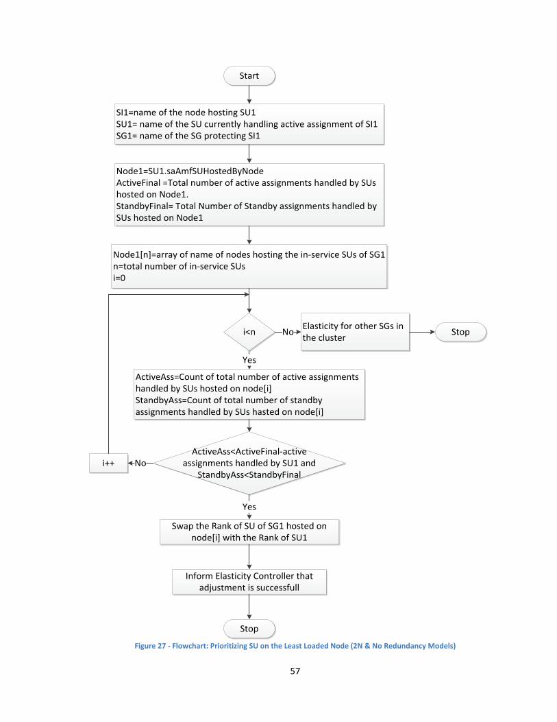
Start

SI1=name of the node hosting SU1SU1= name of the SU currently handling active assignment of SI1SG1= name of the SG protecting SI1

Node1=SU1.saAmfSUHostedByNodeActiveFinal =Total number of active assignments handled by SUs hosted on Node1.StandbyFinal= Total Number of Standby assignments handled by SUs hosted on Node1

Node1[n]=array of name of nodes hosting the in-service SUs of SG1n=total number of in-service SUsi=0

i<n Elasticity for other SGs in the clusterNo Stop

ActiveAss=Count of total number of active assignments handled by SUs hosted on node[i]StandbyAss=Count of total number of standby assignments handled by SUs hasted on node[i]

Yes

ActiveAss<ActiveFinal-active assignments handled by SU1 and

StandbyAss<StandbyFinal

Swap the Rank of SU of SG1 hosted on node[i] with the Rank of SU1

Yes

Inform Elasticity Controller that adjustment is successfull

Stop

i++ No

Figure 27 - Flowchart: Prioritizing SU on the Least Loaded Node (2N & No Redundancy Models)

57

4. For each node in the array ‘node1’

a. The RM Adjustor counts the total number of active assignments and the total number

of standby assignments handled by the SUs hosted on the node.

b. It compares if the total number of active assignments is less than the value of

activeFinal minus the current number of active assignments handled by SU1 and the

total number of standby assignments handled by the node is less than the value of

standbyFinal.

5. If there is such a node, the RM Adjustor selects the one with the least assignments; it

creates a CCB to swap the rank of the SU of the SG1 hosted on this node with the rank

of SU1. In addition, if the SG is not configured to auto adjust, it initiates the SG adjust

administrative operation.

6. If there is no node with lesser assignments than the node hosting SU1, the RM Adjustor

reports to the Elasticity Controller that further adjustments are needed at the cluster level

4.4.2 Workload decrease algorithms

The EE follows the steps defined in the following algorithms to handle workload

decreases in the SG depending on the redundancy model type.

• Merging the SI workload

The steps defined in this algorithm are applicable to an SG of an N-way-Active redundancy

model (see Figure 28). The EE’s Controller determines the redundancy model type of the SG

protecting the SI decreased in workload and calls the RM Adjustor.

1. The RM Adjustor initializes ‘SI1’ with the name of the SI whose workload has

decreased and ‘SG1’ with the name of the SG protecting SI1.

58

2. The RM Adjustor checks if SI1’s ‘saAmfSIPrefActiveAssignments’ attribute value is less

than three and goes to the next step. If it is not less than three, it decreases it by one and

goes ahead.

3. The RM Adjustor checks two conditions before decreasing the

‘saAmfSGNumPrefAssignedSUs’ of SG1.

(1) The product of ‘saAmfSGNumPrefAssignedSUs-1’ and

‘saAmfSGMaxActiveSIsperSU’ value of SG1 is greater than or equal to the sum of

‘saAmfSIPrefActiveAssignments’ of each SI protected by SG1.

(2) The value of ‘saAmfSGNumPrefAssignedSUs-1’ is greater than the value of

‘saAmfSIPrefActiveAssignments’ of each SI of SG1.

a. If one of the two conditions is not satisfied the RM Adjustor goes to Step 4.

b. If both the conditions are satisfied the RM Adjustor decreases the value

‘saAmfSGNumPrefAssignedSUs’ attribute by one. The RM adjustor calls the Buffer

Manager and reports to the Elasticity Controller that the adjustment was successful.

Start

SI1= name of the SI decreased in workloadSG1=SI1.saAmfSIProtectedBySG

SI1.saAmfSIPrefActiveAssignments >=3

DecreaseSI1.saAmfSIPrefActiveAssignments by 1

Yes

(saAmfSGNumPrefAssignedSUs -1)xSG1.saAmfSGMaxActiveSIsperSU>=Sum

of all the assignments of all SIs of SG1No

(SG1.saAmfSGNumPrefAssignedSUs-1)>= for each SI

SI.saAmfSIPrefActiveAssignments

Yes

Component Capability Model > SG1.saAmfSGMaxActiveSIsperSUNo

No

Decrease SG1.saAmfSGNumPrefAssignedSUs

by 1


Inform Elasticity Controller that adjustment was succesful

Stop

If for any SU SU.saAmfSUCurrActiveAssignments = SG1.saAmfSGMaxActiveSIsperSU

Yes

SG1.saAmfSGMaxActiveSIsperSU < Total number of SIs of SG1

Yes

Increase SG1.saAmfSGMaxActiveSIsperSU by 1

Yes

Elasticity on other SG of the ClusterNo Stop

No

No

Figure 28 - Flowchart: Merging the SI Workload (N-way-Active Redundancy Model)

59

4. The RM Adjustor checks the following three conditions to increase

‘saAmfSGMaxActiveSIsperSU’ of SG1. After increasing ‘saAmfSGMaxActiveSIsperSU’

it goes to Step 3.

a. The component compatibility model should be greater than the value of

‘saAmfSGMaxActiveSIsperSU’ attribute of SG1. If not it goes to Step 5.

b. The current number of active assignments of SIs for at least one of the SUs of SG1

must be equal to the value ‘saAmfSGMaxActiveSIsperSU’ attribute of SG1. If not it

goes to Step 5.

c. The value of ‘saAmfSGMaxActiveSIsperSU’ attribute of SG1 must be less than the

total number of SIs protected by the SG1. If not it goes to Step 5.

5. The RM Adjustor informs the Elasticity Controller to try other SGs in the cluster.

• Re-grouping the SIs on less SUs of the SG

The algorithm defines the steps followed by the EE’s RM Adjustor to handle the workload

decrease of the SI protected by the N+M or the N-way redundancy models (see Figure 29).

1. The EE’s RM Adjustor initializes

‘SI1’ with the name of the SI whose workload has increased,

‘SU1’ with the name of the SU currently assigned active for SI1,

‘SG1’ with the name of the SG protecting SI1,

‘ActiveSUs’ pointing to the preferred number of active SUs if the SG1 is of the N+M


redundancy model, and

‘StandbySUs’ indicating the preferred number of standby SUs if SG1 is of the N+M

60


redundancy model.

2. The EE’s RM Adjustor checks if it can decrease the number of SUs of SG by one

without the loss of required active assignments.

3. If it causes the loss of an active assignment, the RM Adjustor will check the component

capability model of the components of the SG to see if the value of the component

capability model is greater than the maximum active SIs per SU of the SG and also

whether the present node capacity is not assigned to the SIs. If all of these conditions are

satisfied the EE will increase the value of maximum active SIs per SU.

4. If the RM Adjustor can decrease the number of SUs without affecting the active

assignments it also checks for the required standby assignments of the SG.

5. If it causes loss of standby assignments, the RM Adjustor will check the component

capability model of the components of the SG to see if the value of the component

capability model is greater than the maximum standby SIs per SU of the SG and also the

RM Adjustor checks whether the present node capacity is not assigned to the SIs. The

RM Adjustor creates a CCB to increase the value of maximum standby SIs per SU.

6. If the RM Adjustor can decrease the number of SUs of the SG without loss of both

required active and standby assignments, it decreases the number of SUs.

7. If the RM Adjustor is not able to free capacity in the SG, it will report to the Elasticity

Controller to try to free the capacity at the cluster level.

61

Start

SI1= name of the SI decreased in workloadSG1=name of the SG protecting SI1

Is SG1 with N-way redundancy model?

ActiveSUs= Preferred number of assigned SUsStandbySUs= Preferred number of assigned SUs

Yes

ActiveSUs=Preferred number of active SUsStandbySUs=Preferred number of standby SUs

No

ActiveSUs x SG1.saAmfSGMaxActiveSiPerSU >

Total number of SIs

Component Capability Model > SG1.saAmfSGMaxActiveSIsperSU NoElasticity for other SGs on

the cluster No

StopIncrease

SG1.saAmfSGMaxActiveSIsperSU by 1

Yes

StandbySUs x SG1.saAmfSGMaxStandbySIsperSU >

Sum(SI.saAmfSIPrefStandbyAssignments)

Yes

Component Capability Model > SG1.saAmfSGMaxStandbySIsperSU

No Elasticity for other SGs on the cluster

StopIncrease

SG1.saAmfSGMaxStandbySIsperSU by 1

Yes

Decrease number of SUs by 1


Inform EE Controller that adjustment is successful

Stop

Figure 29 - Flowchart: Re-grouping the SIs on Less SUs (N+M & N-way Redundancy Models)

• Prioritizing the nodes that serve other SIs

The EE’s RM Adjustor uses the steps defined in this algorithm to handle workload decreases

of SI protected by the 2N or No-Redundancy Redundancy Models (see Figure 30).

1. The EE’s RM Adjustor initializes ‘SI1’ with the name of the SI whose workload has

decreased, ‘SU1’ with the name of the SU currently assigned active for the SI1 and

‘SG1’ with the name of the SG protecting this SI1.

2. The RM Adjustor finds the name of node hosting the SU1 and initializes ‘Node1’. It

then searches for other SUs hosted on Node1 and finds out if they are handling any

assignments. If any of the SUs are handling active assignments, it reports to the

Elasticity Controller for cluster level adjustments. If no SUs are hosted on Node1 that

62

handle any assignments other than SU1 the RM Adjustor must find other in-service SU

of SG1 i.e. on a more loaded node then Node1.

3. It finds all the spare in-service SUs of SG1 and initializes an array ‘node1’ with the

names of nodes hosting them.

4. For each node in the ‘node1’:

a. The RM Adjustor searches for SUs hosted on the node other than the SUs of SG1

and finds out if any of these SUs are handling any assignments. If the RM Adjustor

finds any such node it goes to Step 5 or else it informs the EE Controller for

elasticity action at the cluster level.

5. If there is a node whose hosted SUs are serving SI, it creates a CCB that swaps the rank

of the in-service SU of SG1 with the rank of SU1 and reports to the EE Controller that

the adjustment is successful.

63

Start

SI1=name of the SI decreased in workloadSG1= SI1.saAmfSIProtectedbySGSU1=name of the SU handling active assignmentsNode1=SU1.saAmfSUHostedbyNode

Any SU Hosted except SU1 on

Node1

Each SU Hosted on Node1 except SU1 has saAmfSUNumCurrActiveSIs >0

or SU.saAmfSUNumCurrStandbySIs >0

Yes

Elasticity for other SG in the clusterYes Stop

If SG1.saAmfSGNumPrefInserviceSU

>1

No

No

node1[n]=array of name nodes hosting the in-service SUs of SG1n=to number of in-service SUs in SG1i=0

Yes

i<n No

No

ActiveAss=Count of total number of active assignments handled by SUs hosted on node1[i]StandbyAss=Count of total number of standby assignments handled by SUs hosted on node1[i]

Yes

ActiveAss>0or StandbyAss>0i++ No

Swap the rank of SU of SG1 hosted on node1[i] with the Rank of SU1

Yes

Inform Elasticity Controller that adjustment is successful

Stop Figure 30 - Flowchart: Prioritizing Nodes that Serve other SIs (2N & No Redundancy Models)

4.4.3 Buffer Management algorithms

For the redundancy models where the assignments can be distributed over multiple SUs,

changes in the workload are often handled by changing the number of SUs used for the

distribution. Bringing into service new SUs requires some time because new nodes may need to

be added, the new nodes need the software to be installed and the instantiation of the software

64

may take time. We implement the following algorithm to maintain the ‘in-service-SU-buffer’

and the ‘un-instantiated-SU-buffer’.

• Reservation of resources

When the RM Adjustor increases the number of SUs used for an SI assignment that is

reflected by different attributes depending on the redundancy model, it invokes the Buffer

Manager to adjust the number of SUs of the SG if possible. The Buffer Manager follows the

steps defined in this algorithm to manage the buffers (see Figure 31).

1. The Buffer Manager initializes ‘SG1’ with the name of the SG to be adjusted and

initializes ‘No_Assigned’ with the sum of the preferred number of active SUs and the

preferred number of standby SUs if SG1 is of a N+M redundancy model or else

‘No_Assigned’ is initialized with the preferred number of the assigned SUs in SG1.

2. It initializes ‘Diff1’ by the difference between the value of number of in-service SUs of

SG1 and value of No_Assigned.

3. If Diff1 is greater than or equal to the in-service-SU-buffer, this means that there are

enough in- service SUs then it goes to Step 4 or else it follows Step 5.

4. It initializes ‘Diff2’ by the difference between the number of configured SUs and the

number of in-service SUs of SG1. If Diff2 is greater than or equal to the un-instantiated

SU-buffer, this means that there are enough reserved resources and no adjustments are

needed. If Diff2 is less than the un-instantiated-SU-buffer it follows Step 6.

5. The Buffer Manager increments the number of in-service SUs if there are spare

instantiated SUs in SG1 and goes to Step 3 or else it informs the RM Adjustor to request

the EE Controller to indicate the system administrators or the Cloud management the

need to configure nodes.

65

6. The Buffer Manager checks to see if there are spare nodes in the node group of SG1 to

configure additional SUs. If the number of nodes in the node group of SG1 is greater than

the number of configured SUs then additional SUs can be configured therefore the Buffer

Manager configures a new SU.

7. If the number of SUs in SG1 is equal to the number of nodes in the node group of SG1

that means any new node would require software installation therefore the Buffer

Manager informs the RM Adjustor to report the EE Controller to request the system

administrator or cloud manager to configure new nodes.

Start

SG1=name of the SG to be adjusted

SG1 of N+M redundancy model

No_Assigned = Preferred number of active SUs + Preferred number

of standby SUs of SG1.Yes

No_Assigned = preferred number of assigned SUs of

SG1No

Diff1= SG1.saAmfSGNumPrefInserviceSUs – No_Assigned

SG1.saAmfSGNumPrefInserviceSUs < number of SUs in SG1 No Diff1 >=in-service-SU-

buffer

Increment SG1.saAmfSGNumPrefInserviceSU

s by 1Yes

Inform to configure Nodes

No

Stop

Diff2 = number of configured SUs – number of SUs that can be assigned

Yes

Diff2 > = uninstantiated-SU-

buffer

Sufficient SUs in Buffer

Yes

Stop

Number of SUs of SG1<number of nodes in

Node Group of SG1No

Inform to Configure Nodes

No

Stop

Configure SUs on spare NodesYes

Figure 31 - Flowchart: Buffer Manager (Reservation of Resources)

• Freeing Reserved Resources

When the RM Adjustor decreases the number of SUs used for an assignment, it invokes the

Buffer Manager to release resources in excess if possible. Note that since un-instantiated SUs

do not use resources, the ‘un-instantiated-SU-buffer’ is not adjusted (See Figure 32).

1. The Buffer Manager initializes ‘SG1’ with the name of the SG to be adjusted.

66

2. If SG1 is of an N+M redundancy model, it initializes ‘Diff’ by the difference between the

number of in-service SUs of SG1 and the sum of the preferred number of active and

standby SUs of SG1. If SG1 is not an N+M redundancy model then it initializes ‘Diff’ by

calculating the difference between number of in-service SUs and the number of preferred

assigned SUs of SG1.

3. The Buffer Manager compares if the value of Diff is greater than in-service-SU-buffer. If

yes, it decrements the number of in-service SUs of the SG1 by one and returns to Step 2.

4. The Buffer Manager reports to the RM Adjustor that there are enough SUs of SG1 in the

buffer when the value of Diff is not greater than the in-service-SU-buffer.

Start

SG1=name of the SG to be adjusted

SG1 of N+M redundancy model

Diff=(Number of in-service SUs of

SG1)- sum of number of active SUs and standby SUs of SG1

Yes

Diff=Difference between the number of in-service SUs and number of

assigned SUs of SG1

No

Diff>in-service-SU-buffer

Decrease SG1.saAmfSGNumPrefInserviceSUs by 1

Yes

Inform enough SUs of SG1 in BufferNo Stop

Figure 32 - Flowchart: Buffer Manager (Freeing Reserved Resources)

4.5 Summary

In the chapter, we proposed our solution to manage elasticity and HA with the SA Forum

middleware. The solution uses the elasticity related configuration attributes and the availability

constraints described in Chapter 3. The EE dynamically responds to workload changes according

to the strategies discussed in this chapter. It manipulates the AMF configuration attributes that

67

forces AMF to adjust the amount of resources along with managing HA. The illustration of the

strategies for manipulation of the AMF configuration attributes to handle workload changes is

given in the Appendix.

We have seen in the Related Work section, the cloud controller namely OpenStack [11]

and Heat [12] focus on providing both availability and elasticity at the virtual infrastructure

level. The HA applications usually run in a cluster and their availability is managed by a

middleware through the coordination of redundant resources. In this context, managing elasticity

at a virtual infrastructure level will result in contradictions between the cloud controller and the

middleware. Our solution manages elasticity within AMF of the SA Forum, which is designed to

manage service availability. Thus, we can assume that AMF will maintain the availability of

application services in AMF configuration as long as the AMF configuration remains valid with

respect to the availability constraints. Our solution adjusts the resources by obeying the

availability constraints while manipulating the AMF configuration attributes. Therefore, our

solution with AMF manages the elasticity and the availability of the application services.

The EE strategies proposed assume the workload change of a single SI to adjust the

resources in AMF configuration. They do not handle multiple simultaneous SI workload

changes. The EE strategies can be further developed to handle multiple simultaneous SI

workload changes. In the next chapter, we present our prototype tool and experiments.

68

Chapter 5 - A Prototype of the Elasticity Engine

Based on the EE strategies discussed in Chapter 4, we developed a prototype tool as

proof of our concept. The prototype tool is an application developed in ‘C’ [27]. In this chapter,

we describe the tool and discuss a case study.

5.1 The EE Prototype Architecture

The monitor(s) detect the workload changes represented by an SI in the AMF

configuration and notify the EE. As the workload monitor is still under development by another

student in the research group, we provide the workload increase and decrease through a

Graphical User Interface (GUI). The AMF configuration is rendered in a GUI of EE prototype.

The user clicks on the SI name of the AMF configuration on the GUI of the EE prototype to

indicate the SI workload changes. The EE prototype may also get workload change notifications

from the IMM service [7] when the SI is added or deleted in the AMF configuration. When the

EE prototype receives a notification, of workload change it reads the AMF configuration to

access the redundancy model of the SG and configuration attributes. The EE prototype applies a

combination of the strategies discussed in Chapter 4 depending on the redundancy model of the

SG and the state of the system. The EE prototype writes configuration changes (i.e. CCBs) in the

IMM service. This forces AMF to increase or decrease the resources allocated to the impacted

SI. The EE prototype may also inform the system administrators or cloud managers to increase

the number of nodes in the AMF configuration to speed up further adjustments. Figure 33 shows

the architecture of the EE Prototype tool.

69

Figure 33 - EE Prototype Tool Architecture

Graphical User Interface: the GUI renders graphical outputs and takes inputs from the

user and forwards workload change inputs from the user to the ‘EE_main( )’. The GUI uses the

IMM APIs [7] to read the AMF configuration in the IM to show the configured SIs and SUs with

their names, and indicate the SI-to-SU assignments with identical colors in GUI as shown in

Figure 34. The user clicks on the SI name to indicate the workload change. The user right-clicks

to indicate workload increase and left-clicks to indicate a workload decrease of the SI. The GUI

forwards this input to the ‘EE_main( )’. In addition, when a new SI is created or an SI is deleted,

the GUI is informed to render the information and the information is forwarded to the ‘EE_main(

)’. After the EE adjusts the workload changes, the GUI displays the output of the EE action.

70

Figure 34 – A GUI for rendering an AMF configuration

EE_main( ):the ‘EE_main( )’ determines what type of workload change occurs. It is a

‘Single-SI’ type workload change if the input is from the user and it is a ‘Multiple-SI’ type

workload change if the input is from the IMM service. The ‘EE_main( )’ then calls the

‘SG_type_determine( )’ and passes the name of the impacted SI, elasticity action and workload

change type as parameters. The ‘EE_main( )’ also forwards the output of the EE action to the

GUI after receiving a reply from the ‘SG_type_determine( )’ call.

SG_type_determine( ):upon receiving a call with the parameters ‘SG_type_determine(

)’ uses OM-IMM APIs [7] to read the name of the SG that is protecting the impacted SI and it’s

redundancy model type. The ‘SG_type_determine( )’ decides which ‘RM_Adjustor_Method( )’

to call depending on the redundancy model type of SG, the elasticity action and the workload

change type. After receiving the ‘RM_Adjustor_Method( )’ reply, the ‘SG_type_determine( )’

will carry out one or more of the following actions:

Cluster level adjustment: it will determine other similar types of SGs in the cluster to call

the ‘RM_Adjustor_Method( )’ for them.

Elasticity action Successful: if the EE adjustment was successful it indicates the

‘EE_main( )’ to inform GUI to display “Elasticity Action is Successful”.

71

Configure nodes in the cluster: the ‘SG_type_determine( )’ indicates the ‘EE_main ( )’ to

inform GUI to display “Configure Nodes in Cluster” to inform system management or

cloud management.

RM_Adjustor_Method( ):each of the ‘RM_Adjustor_Method( )’actually implements

the EE algorithms defined in Section 4.4 of the previous chapter. The ‘RM_Adjustor_Method( )’

reads the configuration attribute values of the SG protecting the impacted SI and the execution

state of the system from the IM (using OM-IMM APIs) to determine the CCBs (i.e.

configuration changes). Subsequently, it calls ‘Create_CCB( )’ and passes necessary information

to write CCBs to IMM. This method also calls ‘Buffer_Manager( )’ to manage the number of

SUs in SG according to the ‘in-service-SUs-buffer’ and ‘un-instantiated-SU-buffer’.

Create_CCB( ):the ‘Create_CCB( )’ function uses the OM-IMM APIs [7] to write the

CCBs in IMM. After the CCB implementation, it returns to the calling function.

Buffer_Manager( ):the ‘Buffer_Manager( )’ implements the algorithms defined in

Section 4.4 of Chapter 4. The ‘Buffer_Manager( )’ reads the IM using the IMM APIs [7] to

check the number of SUs in the SG. If the number of SUs in the SG are not enough according to

the ‘in-service-SU-buffer’ and un-instantiated-SU-buffer’, it calculates CCBs and calls the

‘Create_CCB( )’ to write the CCBs in IMM.

5.2 Experiment Test-bed Set-up

For experimentation we use OpenSAF 4.3 [6] middleware as it is an open source

middleware that implements the SA Forum [8] specifications. The EE prototype tool is deployed

on a VM in the VMware player [28] on a Host with Intel® Core™ i7 -2600 CPU 340 GHz,

RAM 16GB and 64-bit Windows operating system [29]. The VM Player is free for personal use

and also allows us to create up to 17 virtual processors, 8TB virtual disks and 64 GB memory per

72

VM [28] which is enough for the experimentation. We create five VMs with the Ubuntu 10.04

operating system [30] and install OpenSAF 4.3 [6] on each of them.

For the communication between cluster nodes we use Transparent Inter-Process

Communication protocol (TIPC) [31]. The VMs in the cluster are isolated from any external

network to allow only internal communication between the VMs through TIPC. Since the five

VMs in the cluster closely communicate with each other we can run the EE prototype tool on any

one of the VMs.

5.3 A Case Study

In this section we discuss a case study used, to experiment with the EE prototype tool.

The case study is a system consisting of two applications. The system configuration is shown in

Figure 35. The application ‘safApp=AmfDemo1’ consists of one SI

‘safSi=AmfDemo,safApp=AmfDemo1’ protected by SG ‘safSg=AmfDemo,safApp=AmfDemo1’

with a N-way-Active redundancy model. The application ‘safApp=AmfDemo2’ consists of two

SIs namely ‘safSi=AmfDemoSi,safApp=AmfDemo2’ and

‘safSi=AmfDemoSi1,safApp=AmfDemo2’ protected by SG

‘safSg=AmfDemo,safApp=AmfDemo2’ with a N+M redundancy model. The two SGs consist of

five SUs configured on separate AMF nodes. Each AMF node corresponds to a VM in the VM

player.

73

Figure 35 – System Configuration for the Case Study

5.4 Experiments with the EE Prototype Tool

In this section we test the behavior of the EE when the workload of the applications

represented by the SI increases or decreases.

5.4.1 Workload increase

In this subsection we test the EE prototype for a workload increase with two test cases:

when the workload of the SI protected by an SG with an N-way-Active redundancy model

increases, and when the workload of the SI protected by an SG with an N+M redundancy model

increases.

Test case: Workload increase for the SG with an N-way-Active redundancy model

The prototype tool reads the initial system configuration and displays it on the GUI as shown

in Figure 34. It displays the SUs of the two SGs and the SIs representing application’s

workloads. The SIs and the assigned SUs of ‘safApp=AmfDemo1’ application are in blue.

The SIs and the assigned SUs of the ‘safApp=AmfDemo2’ application are in green. The GUI

74

also displays the current number of active assignments and standby assignments each SU

handles (see Figure 34).

Figure 36 gives ‘safSg=AmfDemo,safApp=AmfDemo1’ SG object’s configuration

attribute values and Figure 37 gives ‘safSi=AmfDemo,safApp=AmfDemo1’ SI object’s

configuration attribute values. We run ‘immlist’ command in OpenSAF [8] [6] to list these

attribute values.

Figure 36 - ‘safSg=AmfDemo,safApp=AmfDemo1’ SG object before the EE action

Figure 36 shows that ‘safSg=AmfDemo,safApp=AmfDemo1’ SG consists of five in-service

SUs (indicated by ‘saAmfSGNumPrefInserviceSUs’), two assigned SUs (indicated by

‘saAmfSGNumPrefAssignedSUs’) and maximum active SIs per SU is one (indicated by

‘saAmfSGMaxActiveSIsperSU’). Figure 37 shows that ‘safSi=AmfDemo,safApp=AmfDemo1’

SI is assigned to two SUs (indicated by ‘saAmfSIPrefActiveAssignments’).

75

Figure 37 - ‘safSi=AmfDemo,safApp=AmfDemo1’ SI object before the EE action

To test the EE’s behavior for workload increases in the SG with an N-way-Active

redundancy model, we right-click on ‘safSi=AmfDemo,safApp=AmfDemo1’ SI on the GUI

shown in Figure 34. The right-click event of the GUI calls the ‘EE_main( )’ and passes the SI

name and the workload increase as parameters.

The ‘EE_main( )’ determine this as a workload increase with the workload change of type

Single-SI. The ‘SG_type_determine( )’ uses IMM APIs [7] to read the IM. It determines that

the SI is protected by SG with an N-way-Active redundancy model and calls the specific

‘RM_Adjustor_Method( )’ to adjust resources. This ‘RM_Adjustor_Method( )’ uses the

‘Spreading the SI workload’ strategy explained in Chapter 4. Before increasing capacity it

checks if the SI’s ‘saAmfSIPrefActiveAssignments’ attribute value is less than the SG’s

‘saAmfSGNumPrefAssignedSUs’ attribute value and if it is not less, the

‘RM_Adjustor_Method( )’checks if it can increase the number of assigned SUs. The number

of in-service SUs for the SG is five (see Figure 36); hence it calls ‘Create_CCB( )’ to write a

CCB in IMM to increase the assigned SUs to three. The ‘RM_Adjustor_Method( )’ then

gives a call to the ‘Buffer_Manager( )’ because the number of assigned SUs of the SG has

76

changed. The ‘Buffer_Manager( )’ reads the IM and determines that the number of in-service

SUs are not enough and informs the controller to increase the ‘number of nodes for future

workload increases’ and returns to the ‘RM_Adjustor_Method( )’. Subsequently, the

‘RM_Adjustor_Method( )’ reads that the active assignments of the SI are two (see Figure 37)

and the assigned SUs are three (see Figure 39) and checks to see if the SG has capacity

before it calls the ‘Create_CCB( )’ to write a CCB in IMM to increase the SI active

assignments to three in the IM. It checks by calculating whether the active capacity (i.e.

‘saAmfSGMaxActiveSIsperSU x saAmfSGNumPrefAssignedSUs’) is greater than the sum of

the active SI assignments. Thus after the CCB implementation the system configuration has

capacity to handle three active assignments of the SI, hence the ‘RM_Adjustor_Method( )’

calls the ‘Create_CCB( )’ to write a CCB in IMM to increase the SI assignment to three. This

CCB forces AMF to assign the SI active assignment to the unassigned SU. The

‘RM_Adjustor_Method( )’ returns ‘Elasticity action is successful’ to the calling function.

Figure 38 gives the output of the EE when the SI is clicked to indicate a workload increase.

Figure 39 and Figure 40 show the SG and SI object’s attributes after the EE action.

Figure 38 - System Configuration after EE and AMF actions for the workload increase in a SG with N-way-Active

redundancy model

77

Figure 39 - ‘safSg=AmfDemo,safApp=AmfDemo1’ SG object after the EE action

Figure 40 - ‘safSi=AmfDemo,safApp=AmfDemo1’ SI object after the EE action

Test case: Workload increase for the SG with an N+M redundancy model

To test this case we use the system configuration results of the previous test case. Figure 38

shows the system configuration to test the behavior of the EE when the workload of SI

protected by SG using N+M redundancy model increases.

The list of configuration attribute values of the ‘safSg=AmfDemo,safApp=AmfDemo2’ SG

object with the N+M redundancy model is shown in Figure 41. The SG has one active SU

78

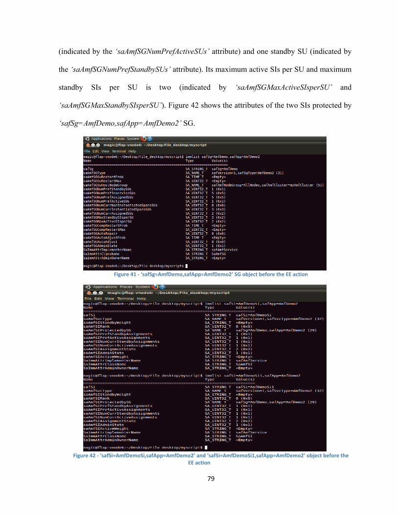
(indicated by the ‘saAmfSGNumPrefActiveSUs’ attribute) and one standby SU (indicated by

the ‘saAmfSGNumPrefStandbySUs’ attribute). Its maximum active SIs per SU and maximum

standby SIs per SU is two (indicated by ‘saAmfSGMaxActiveSIsperSU’ and

‘saAmfSGMaxStandbySIsperSU’). Figure 42 shows the attributes of the two SIs protected by

‘safSg=AmfDemo,safApp=AmfDemo2’ SG.

Figure 41 - ‘safSg=AmfDemo,safApp=AmfDemo2’ SG object before the EE action

Figure 42 - ‘safSi=AmfDemoSi,safApp=AmfDemo2’ and ‘safSi=AmfDemoSi1,safApp=AmfDemo2’ object before the

EE action

79

To test the EE’s behavior for a workload increase for the SG with an N+M redundancy

model, we right-click on the name of ‘safSi=AmfDemoSi,safApp=AmfDemo2’ SI on the GUI

shown in Figure 38. The right-click event of the GUI calls the ‘EE_main( )’ and passes the SI

name and the workload increase as parameters.

The ‘EE_main( )’ determines the workload of the SI is increased and is of the Single-SI type.

The ‘SG_type_determine( )’ uses the IMM APIs [7] to read the

‘safSi=AmfDemoSi,safApp=AmfDemo2’ SI attributes in the IM and finds that the

‘safSg=AmfDemo,safApp=AmfDemo2’ SG is protecting this SI (see Figure 42). It determines

the redundancy model type of the SG is N+M redundancy model and calls the

‘RM_Adjustor_Method( )’. The ‘RM_Adjustor_Method( )’ follows the strategy of

‘Distributing the SIs over more SUs’ explained in Chapter 4. The ‘RM_Adjustor_Method( )’

checks if any SI assignments will be lost if it decreases the number of active SI assignments

each SU of the SG can handle (i.e ‘saAmfSGMaxActiveSIsperSU’) to distribute the workload

to more SIs. In the current system configuration, it calculates the available active capacity

excluding the capacity that will be lost after decreasing the SG’s

‘saAmfSGMaxActiveSIsperSU’ attribute value by multiplying attribute values of

‘saAmfSGMaxActiveSIsperSU-1’ and ‘saAmfSGNumPrefActiveSUs’ of the SG which gives

one (see Figure 41) but the capacity required is two (see Figure 42). Hence, the

‘RM_Adjustor_Method( )’ cannot decrease the SG’s ‘saAmfSGMaxActiveSIsperSU’ attribute

value by one. The ‘RM_Adjustor_Method( )’ tries to increase the number of active SUs if

there are spare in-service SUs available of the SG. The SG has three spare in-service SUs

(see Figure 41) hence the ‘RM_Adjustor_Method( )’ increases the number of

‘saAmfSGNumPrefActiveSUs’ by one by calling the ‘Create_CCB( )’ and calls the

80

‘Buffer_Manager( )’. The ‘Buffer_Manager( )’ determines that the number of SUs are not

enough hence it returns, ‘Configure Nodes in the cluster for future workload increase’ to the

calling method. The ‘RM_Adjustor_Method( )’ again checks if any SI assignments will be

lost if it decreases the number of SIs each SU can handle of the SG. The available active

capacity will be two after decreasing the attribute ‘saAmfSGMaxActiveSIsperSU’ value to

one of the SG. Hence, the ‘RM_Adjustor_Method( )’ calls the ‘Create_CCB( )’ to initialize a

CCB in IMM to decrease the value of ‘saAmfSGMaxActiveSIsperSU’ by one. For the standby

assignments of the SI, the ‘RM_Adjustor_Method( )’ checks if any SI assignments will be

lost if it decreases the number of standby SI assignments each SU can handle (i.e.

‘saAmfSGMaxStandbySIsperSU’) of the SG. It calculates the available standby capacity

excluding the capacity that will be lost after decreasing the ‘saAmfSGMaxStandbySIsperSU’

by multiplying ‘saAmfSGMaxStandbySIsperSU-1’ and ‘saAmfSGNumPrefStandbySUs’

attribute values of the SG. For the above example, it is one and the required capacity is two

(see Figure 41). Hence, the ‘RM_Adjustor_Method( )’ cannot decrease the

‘saAmfSGMaxStandbySIsperSU’ by one of the SG. It tries to increase the number of standby

SUs, if there are spare in-service SUs available. This SG has two spare in-service SU (see

Figure 44) hence the ‘RM_Adjustor_Method( )’ increases the number of

‘saAmfSGNumPrefStandbySUs’ by one of the SG. Then the ‘RM_Adjustor_Method( )’ calls

the ‘Create_CCB( )’ to initialize a CCB in IMM to decrease the

‘saAmfSGMaxStandbySIsperSU’ by one of SG. This forces AMF to distribute the standby SI

assignments on more SUs. The ‘RM_Adjustor_Method( )’ compares to find, if the active and

standby assignments handled by the SUs have reduced after applying the CCBs. The

assignments of the SUs of the SG have reduced as shown in Figure 43, hence it reports that

81

the ‘Elasticity Action is Successful’. Figure 43 gives the output of the EE, when we click the

SI to indicate the workload increase. Figure 44 and Figure 45 show the SG object’s attributes

after the EE action.

Figure 43 - System Configuration after EE and AMF actions for workload increase in a SG with N+M redundancy

model


5.4.2 Workload decrease

In this subsection, we test the EE prototype tool for a workload decrease with two test

cases: when the workload of the SI protected by an SG with an N-way-Active redundancy model

82

decreases, and when the workload of the SI protected by an SG with an N+M redundancy model

decreases.

Test case: Workload decrease for an SG with an N-way-Active redundancy model

We use the system configuration results of the previous test case as shown in Figure 43 to

test the workload decrease for an SG with an N-way-Active redundancy model.

The list of configuration attribute values of ‘safSg=AmfDemo,safApp=AmfDemo1’ SG object

with an N-way-Active redundancy model is shown in Figure 39. The SG has three assigned

SUs (indicated by the ‘saAmfSGNumPrefAssignedSUs’ attribute) and five in-service SUs

(indicated by the ‘saAmfSGNumPrefInserviceSUs’ attribute). Its maximum active SIs per SU

(i.e. ‘saAmfSGMaxActiveSIsperSU’) is one. Figure 40 shows the

‘safSi=AmfDemo,safApp=AmfDemo1’ SI object’s attributes. The SI is assigned to three SUs

(indicated by ‘saAmfSIPrefActiveAssignments’).

To test the EE’s behavior for workload decreases for the SG with an N-way-Active

redundancy model, we left-click on the name of ‘safSi=AmfDemo,safApp=AmfDemo1’ SI on

the GUI shown in Figure 43. The left-click event of the GUI calls the ‘EE_main( )’ and

passes the SI name and the workload decrease as parameters.

The ‘EE_main( )’ determines a workload decrease and the workload change of type Single-

SI. The ‘SG_type_determine( )’ uses IMM APIs [7] to read the IM. It determines that the SI

is protected by ‘safSg=AmfDemo,safApp=AmfDemo1’ SG with an N-way active redundancy

model (see Figure 40). The ‘SG_type_determine( )’ accordingly calls the

‘RM_Adjustor_Method( )’ to handle the workload decrease in the SG. The

‘RM_Adjustor_Method( )’ follows the strategy of the ‘Merging the SI workload’ explained

in Chapter 4. This ‘RM_Adjustor_Method( )’ reads the IM to determine that the SI object has

83

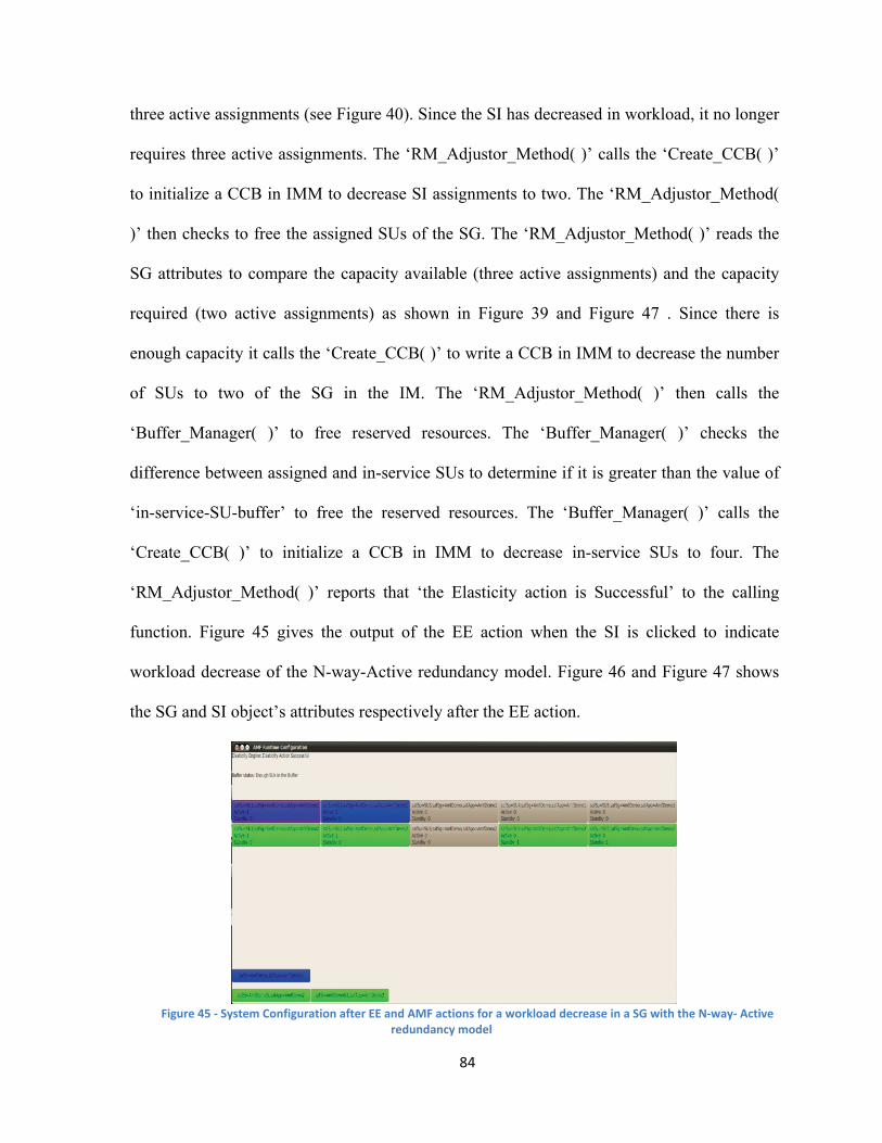
three active assignments (see Figure 40). Since the SI has decreased in workload, it no longer

requires three active assignments. The ‘RM_Adjustor_Method( )’ calls the ‘Create_CCB( )’

to initialize a CCB in IMM to decrease SI assignments to two. The ‘RM_Adjustor_Method(

)’ then checks to free the assigned SUs of the SG. The ‘RM_Adjustor_Method( )’ reads the

SG attributes to compare the capacity available (three active assignments) and the capacity

required (two active assignments) as shown in Figure 39 and Figure 47 . Since there is

enough capacity it calls the ‘Create_CCB( )’ to write a CCB in IMM to decrease the number

of SUs to two of the SG in the IM. The ‘RM_Adjustor_Method( )’ then calls the

‘Buffer_Manager( )’ to free reserved resources. The ‘Buffer_Manager( )’ checks the

difference between assigned and in-service SUs to determine if it is greater than the value of

‘in-service-SU-buffer’ to free the reserved resources. The ‘Buffer_Manager( )’ calls the

‘Create_CCB( )’ to initialize a CCB in IMM to decrease in-service SUs to four. The

‘RM_Adjustor_Method( )’ reports that ‘the Elasticity action is Successful’ to the calling

function. Figure 45 gives the output of the EE action when the SI is clicked to indicate

workload decrease of the N-way-Active redundancy model. Figure 46 and Figure 47 shows

the SG and SI object’s attributes respectively after the EE action.

Figure 45 - System Configuration after EE and AMF actions for a workload decrease in a SG with the N-way- Active

redundancy model

84


Figure 47 - ‘safSi=AmfDemo,safApp=AmfDemo1’ SG object after the EE action

Test case: Workload decrease for the SG with an N+M redundancy model

We use the system configuration results of the previous test case as shown in Figure 45 to

test the workload decrease for an SG with an N+M redundancy model.

85

The list of configuration attribute values of ‘safSg=AmfDemo,safApp=AmfDemo2’ SG object

with the N+M redundancy model is shown in Figure 44. The SG has five in-service SUs

(indicated by the ‘saAmfSGNumPrefInserviceSUs’ attribute), two active SUs (indicated by

‘saAmfSGNumPrefActiveSUs’) and two standby SUs (indicated by

‘saAmfSGNumPrefStandbySUs’). Its maximum active SIs per SU (i.e

‘saAmfSGMaxActiveSIsperSU’) is one and its maximum standby SIs per SU is one

(‘saAmfSGMaxStandbySIsperSU’). Figure 42 shows SIs protected by

‘safSg=AmfDemo,safApp=AmfDemo2’ SG with an N+M redundancy model.

We left-click on ‘safSi=AmfDemoSi,safApp=AmfDemo2’ on the GUI shown in Figure 45 to

test the EE behavior when there is a decrease in workload represented by an SI protected by

the SG with an N+M redundancy model. The left-click event of the GUI calls the ‘EE_main(

)’ and passes the SI name and the workload decrease as parameters.

The ‘EE_main( )’ determines a workload decrease and the workload change of type Single-

SI. The ‘SG_type_determine( )’ uses IMM APIs [7] to read the IM. It determines that

‘safSi=AmfDemoSi,safApp=AmfDemo2’ is protected by

‘safSg=AmfDemo,safApp=AmfDemo2’ SG (see Figure 45) with an N+M redundancy model

and accordingly calls the ‘RM_Adjustor_Method( )’. This ‘RM_Adjustor_Method( )’ uses

‘Re-grouping the SIs on less SUs of the SG’ strategy explained in Chapter 4. According to

the strategy, it checks if it can decrease the number of SUs without losing active assignments

by multiplying SG’s ‘saAmfSGMaxActiveSIsperSU’ and ‘saAmfSGNumPrefActiveSUs-1’

attribute values. The calculated active capacity is one (see Figure 44) which is not enough for

the two SIs. It then checks the required constraining attributes (i.e.

‘saAmfCompNumMaxActiveCSIs’ [4] ) to increase the maximum number of SIs that can be

86

assigned to each SU in the SG (i.e. the ‘saAmfSGMaxActiveSIsperSU’ attribute). The

component capability model allows to increase the ‘saAmfSGMaxActiveSIsperSU’ by one

hence it calls ‘Create_CCB( )’ to write a CCB in IMM to increase it to two. The

‘RM_Adjustor_Method( )’ then tries to decrease the number of active SUs of the SG. The

available active capacity in the SG is four and the required active capacity is two active SI

assignments. The ‘RM_Adjustor_Method( )’ calls the ‘Create_CCB( )’ to write the CCB in

IMM to increase decrease the number of active SUs to one. The ‘RM_Adjustor_Method( )’

then tries to decrease the standby SUs. It calculates the available capacity after decreasing

one standby SU of the SG will be one standby assignment (see Figure 44) but the required

capacity is two standby SI assignments. The ‘RM_Adjustor_Method( )’ will try to increase

the maximum standby SIs per SU of the SG (i.e. ‘saAmfSGMaxStandbySIsperSU’) by

checking if the component capability model allows (i.e. ‘saAmfCompNumMaxStandbyCSI’

[4]) to increase it by one. It calls the ‘Create_CCB( )’ to write a (see Figure 44 and Figure

43) CCB in IMM to increase the number of maximum standby SI assignments per SU of the

SG. The ‘RM_Adjustor_Method( )’ then checks if it can decrease the number of standby

SUs. The available standby capacity is four standby assignments and required standby

capacity is two standby SI assignments. It then calls the ‘Create_CCB( )’ to write a CCB in

IMM to decrease the number of standby SUs by one of the SG and calls the

‘Buffer_Manager( )’ to free any in-service SUs. Figure 48 gives the output of the EE when SI

is clicked to indicate workload decrease. Figure 49 shows the SG object’s attribute values.

87

Figure 48 - System Configuration after EE and AMF actions for workload decrease in an SG with N+M redundancy

model

Figure 49 - ‘safSg=AmfDemo,safApp=AmfDemo2’ SG after the EE action

5.4.3 Cluster Level Adjustments

In this section we will execute the EE to test ‘Cluster level Adjustment’ when workload

changes for a SI that is protected by one of the SGs in the cluster.

88

Figure 50 - System Configuration to test Cluster Level Adjustments

When we execute the EE, it reads the configured AMF configuration and displays it on

the GUI. Figure 50 shows the system configuration. The ‘safSg=AmfDemo,safApp=AmfDemo1’

and ‘safSg=AmfDemo,safApp=AmfDemo2’ are configured on the same five nodes. They share

resources with each other. The ‘safSg=AmfDemo,safApp=AmfDemo2’ SG is using four SUs

configured on the nodes as shown in Figure 50. If there is any change in the workload

represented by the SI protected by the ‘safSg=AmfDemo,safApp=AmfDemo2’ SG the EE will

adjust the SI-to-SU assignments on the other SG at the cluster level to handle the workload

change. We demonstrate the same behavior of the EE in this test case.

We right-click ‘safSi=AmfDemoSi,safApp=AmfDemo2’ SI on the GUI shown in Figure

50 to indicate a workload increase. The right-click event of the GUI calls the ‘EE_main( )’ and

passes the SI name and workload increase as parameters. The ‘EE_main( )’ determines a

workload increase and the workload change type is Single-SI. The ‘SG_type_determine( )’ uses

the IMM APIs [7] to read the IM. It finds that the SI is protected by

89

‘safSg=AmfDemo,safApp=AmfDemo2’ SG with the N+M redundancy model and calls the

‘RM_Adjustor_Method( )’. This ‘RM_Adjustor_Method( )’ uses the ‘Distribute the SIs over

more SUs’ strategy explained in Chapter 4. This ‘RM_Adjustor_Method( )’ cannot handle the

workload increase in ‘safSg=AmfDemo,safApp=AmfDemo2’ SG because all the SIs of the SG

are distributes and the ‘RM_Adjustor_Method( )’ cannot spread the SIs any more (see Figure

50). This ‘RM_Adjsutor_Method( )’ reports the ‘SG_type_determine( )’ that the adjustment

needs to be done at the cluster level. The ‘SG_type_determine( )’ uses the ‘Cluster level

adjustment’ strategy explained in Chapter 4 to increase the resources allocated to

‘safSi=AmfDemoSi,safApp=AmfDemo2’ SI. According to the ‘Cluster level adjustment’ strategy,

the ‘SG_type_determine( )’ reads the IM using the IMM APIs to determine other SGs in the

cluster that are sharing resources with ‘safSg=AmfDemo,safApp=AmfDemo2’. It finds that the

SUs of ‘safSg=AmfDemo,safApp=AmfDemo1’ are also configured on the same group of nodes in

the cluster (see Figure 50). It determines that ‘safSg=AmfDemo,safApp=AmfDemo1’ is of N-

way-Active redundancy model and calls the ‘RM_Adjustor_Method( )’ accordingly. This

‘RM_Adjustor_Method( )’ determines the required configuration changes to spread the workload

of ‘safSi=AmfDemo,safApp=AmfDemo1’ from two SUs namely

‘safSu=SU1,safSg=AmfDemo,safApp=AmfDemo1’ &

‘safSu=SU2,safSg=AmfDemo,safApp=AmfDemo1’ to three SUs. It calls the ‘Create_CCB( )’ to

write the CCBs in IMM. This gives the impacted SI (safSi=AmfDemoSi,safApp=AmfDemo2)

more capacity to use on nodes. The EE displays that the ‘EE action was successful’ on the GUI

as shown in Figure 51.

90

Figure 51 - System Configuration after EE and AMF action for Cluster Level Adjustments

5.5 Summary

In this chapter we described the EE prototype and tested the EE strategies. We briefly

demonstrated its usage through a simple case study. Further testing of the EE is required as

future work. Moreover, more realistic case studies should be considered.

91

Chapter 6 - Conclusion and Future Work

6.1 Conclusion

The objective of this thesis was to propose a solution to manage elasticity and availability

in the application level. Elasticity is a key requirement in cloud computing and generally cloud

services are believed to be “available” all the time. In the thesis we reviewed the facts that

existing cloud solutions such as OpenStack [11] and Heat [12] handle elasticity and availability

at the level of VMs. These solutions equate the application and its workload to the VMs running

the applications. HA applications are typically composed of redundant resources in a cluster

managed by a middleware. The management of elasticity and HA of such applications in the

cloud at the virtual infrastructure level will result in contradictions between the cloud controllers

and the middleware. In this thesis, we proposed an EE that manages application level elasticity

within AMF designed to manage service availability.

We defined ‘Single-SI’ and ‘Multiple-SI’ types of workload changes in an AMF

configuration to characterize the potential changes in workloads and determined the AMF

configuration attributes related to elasticity and the attributes constraining them. We presented

the overall architecture for HA and elasticity management using the SA Forum middleware.

Further, we proposed the architecture of the EE that consists of the Controller, the RM Adjustor

and Buffer Manager. We also presented the working components of each part of the EE. AMF

allows the manipulation of its configuration. The EE proposed in this thesis manipulates the

AMF configuration that forces AMF to increase the resources or decrease resources in the

configuration. Thus AMF and OpenSAF as a middleware can be a promising solution for

92

managing application availability in the cloud; however the integration of the EE with cloud

orchestration needs further work.

In the thesis, we have defined strategies to handle the workload increase and decrease in

an AMF configuration. We also defined a buffer management strategy for reserving or freeing

resources in an AMF configuration to handle future workload changes and a cluster level

adjustment strategy to adjust resources in the cluster to handle the workload changes. The EE

follows one or more of the proposed strategies according to the redundancy model of the SG

protecting the impacted SI and the execution status of the system to manipulate the AMF

configuration. Finally, we developed the EE prototype that implements the proposed strategies

and architecture, and tested it.

6.2 Future Work

The solution presented in this thesis has been prototyped and tested using OpenSAF [6].

However, as the workload monitor is under development the workload increase and decrease is

provided through a user interface. The workload monitor requires further research by itself as

low level monitoring of processes and threads in the nodes of cluster need to be mapped into the

AMF configuration and SI-workload. Measuring the real workload and comparing it with actual

resource capacities available in the nodes will also provide more refined selection of elasticity

strategies.

The EE strategies used so far have not been tested for multiple simultaneous SI workload

changes. In future work, the EE can be extended to handle this issue. The strategies we propose

are more focused to provision resources but policies that consider the Service Level Agreements

(SLAs) and pricing of resources could be considered as future extension. Also, efficient

93

workload prediction policies could be incorporated so that the EE can handle changes more

efficiently.

94

Reference

[1] M. Toeroe and T. Francis, Service Availability: Principles and Practice. Wiley, 2012.

[2] A. Kanso, “Automated Configuration Design and Analysis for Service by,” no. May, 2012.

[3] N. R. Herbst, S. Kounev, and R. Reussner, “Elasticity in Cloud Computing : What It Is , and What It Is Not,” pp. 23–28.

[4] Service AvailabilityTM Forum, “Application Interface Specification,Availability Management Framework, SAI-AIS-AMF-B.04.01.,” pp. 1–452, 2011.

[5] Service AvailabilityTM Forum, “Official homepage.” [Online]. Available: htt://www.saforum.org.

[6] The Open Service availability Framework, “‘Official homepage.’ [Online]. Available: http://www.opensaf.org.”[Online]. Available: http://www.opensaf.org.

[7] Service AvailabilityTM Forum, “Application Interface Specification, Information Model Management Service SAI-AIS-IMM-A.02.01.,” pp. 1–152.

[8] Service AvailabilityTM Forum, “Service Availability Interface, Overview,SAI-Overview-B.05.02.,” 2011.

[9] M. Hamilton(1999), Marc Hamilton (1999) Software Development: A Guide to Building Reliable Systems p.48. .

[10] J. Sermersheim, “Lightweight Directory Access Protocol (LDAP): The Protocol,” The Internet Engineering Task Force. pp. 1–69, 2006.

[11] The OpenStack Cloud Operating System, “‘Official homepage.’ [Online]. Available: https://www.openstack.org/.”.

95

[12] “Heat available at https://wiki.openstack.org/wiki/Heat D. Michelino, J.C Leon, and L.F. Alvarez, ‘Implementing and testing of OpenStack Heat’no. September,2013.”.

[13] “Ceilometer available at https://wiki.openstack.org/wiki/Ceilometer.” .

[14] “Ceilometer available at https://wiki.openstack.org/wiki/Ceilometer.” .

[15] P. Marshall, K. Keahey, and T. Freeman, “Elastic Site: Using Clouds to Elastically Extend Site Resources,” 2010 10th IEEE/ACM Int. Conf. Clust. Cloud Grid Comput., pp. 43–52, 2010.

[16] M. a. Murphy, B. Kagey, M. Fenn, and S. Goasguen, “Dynamic Provisioning of Virtual Organization Clusters,” 2009 9th IEEE/ACM Int. Symp. Clust. Comput. Grid, pp. 364–371, 2009.

[17] X. Chaoqun, Z. Yi, and Z. Wei, “A Load Balancing Algorithm with Key Resource Relevance for Virtual Cluster,” Int. J. Grid Distrib. Comput., vol. 6, no. 5, pp. 1–16, Oct. 2013.

[18] Y. Zhang, G. Huang, X. Liu, and H. Mei, “Integrating Resource Consumption and Allocation for Infrastructure Resources on-Demand,” 2010 IEEE 3rd Int. Conf. Cloud Comput., pp. 75–82, Jul. 2010.

[19] J. Yang, J. Qiu, and Y. Li, “A Profile-Based Approach to Just-in-Time Scalability for Cloud Applications,” 2009 IEEE Int. Conf. Cloud Comput., pp. 9–16, 2009.

[20] N. Roy, A. Dubey, and A. Gokhale, “Efficient Autoscaling in the Cloud Using Predictive Models for Workload Forecasting,” 2011 IEEE 4th Int. Conf. Cloud Comput., pp. 500–507, Jul. 2011.

[21] J. Y. Lee and S. D. Kim, “Software Approaches to Assuring High Scalability in Cloud Computing,” 2010 IEEE 7th Int. Conf. E-bus. Eng., pp. 300–306, Nov. 2010.

[22] T. C. Chieu, A. Mohindra, A. a. Karve, and A. Segal, “Dynamic Scaling of Web Applications in a Virtualized Cloud Computing Environment,” 2009 IEEE Int. Conf. E-bus. Eng., pp. 281–286, 2009.

96

[23] T. S. Somasundaram and K. Govindarajan, “A Broker Based Architecture for Adaptive Load Balancing and Elastic Resource Provisioning and Deprovisioning in Multi-tenant,” pp. 561–573.

[24] Saheli_PhD_S2012_2, “A Model Based Framework for Service Availability Management in The Department of Elaectrical and Computer Engineering Presented in Partial Fulfillment of the Degree of Philosophy at Concordia University Montreal,Canada.,” no. April, 2012.

[25] OMG, “Object Constraint Language,Version 2.2 - http://www.omg.org/spec/OCL/2.2.PDF,” vol. 03, no. February, 2010.

[26] “VLC media player available at http://www.videolan.org/index.html.” .

[27] D. M. R. Brian W Kernighan, The C programming language. 1988, pp. 1–217.

[28] T. Vm. P. VMware, “VMware Player.” [Online]. Available: http://www.vmware.com/products/player.

[29] Windows, “Windows.” .

[30] Ubuntu, “Ubuntu 10.04.” [Online]. Available: http://www.ubuntu.com/.

[31] “TIPC.” [Online]. Available: http://tipc.sourceforge.net/.

97

Appendix

A number of examples are provided to illustrate configuration changes in response to a

workload change made by the EE as explained in Chapter 4. Figure 52 shows an example of

configuration of an SG with a 2N redundancy model.

I. Workload changes of an SG with a 2N redundancy model

• Workload increase of type Single-SI

Configuration:

Attribute Names SG1 SG2

Ordered List of SUs in SG {SU1, SU2, SU3} {SU1, SU2, SU3}

Ordered List of SIs {SI1, SI2} {SI1, SI2}

saAmfSGMaxActiveSIsperSU 2 2

saAmfSGMaxStandbySIsperSU 2 2

saAmfSGAutoAdjust SA_TRUE SA_TRUE

component capability model 2_active_or 2_standby 2_active_or 2_standby

Figure 52 - System Configuration of SGs with a 2N redundancy model before CCB implementation

98

In the system configuration shown in Figure 52, assume that the workload

represented by SI-3 increases. The EE’s Elasticity Controller receives a workload

increase signal of SI-3 and determines that SI-3 is protected by SG2 with a 2N

redundancy model. The EE’s Elasticity Controller will accordingly call the RM

Adjustor method to adjust the workload increase.

The EE’s RM Adjustor method uses the strategy of ‘Prioritizing the SU on the least

loaded node’ as explained in Chapter 4. The RM Adjustor reads the name of SU to

which SI-3 is currently assigned. It then accesses the SU’s attribute

‘saAmfSUHostedByNode’ in the IM using IMM APIs. The RM Adjustor then

calculates the total number of active and standby SI assignments currently handled by

SUs hosted on each node hosting the in-service SUs of SG2. For the system

configuration shown in Figure 52 SI-3 is assigned to SU1 of SG2. The SG2’s SU1 is

hosted on node ‘Node1’. This ‘Node1’ also hosts SU1 of SG1 and the total numbers

of active assignments are three and standby assignments are 0. Similarly the RM

Adjustor counts the total number of assignments handled by the SUs hosted by each

node hosting the in-service SUs of SG2. The RM Adjustor then compares the

assignments to get the node that will have the least number of assignments after the

assignments of current active SU1 of SG2 are assigned to it. For the system

configuration shown in Figure 52, Node3 has the least number of assignments i.e.

zero and will handle only two active assignments after the in-service SU3 of SG2 is

ranked higher. The least loaded node will have the maximum free capacity which the

loaded SI can use. The RM Adjustor creates CCBs to swap the ranks of SU3 with

99

SU1 of SG2. Figure 53 shows the system configuration of the SGs after the EE and

AMF actions.

CCBs: saAmfSURank (SU1) of SG2: 3

saAmfSURank (SU3) of SG2: 1

Figure 53 - System Configuration of SGs with a 2N redundancy model after CCB implementation (workload

increase)

• Workload decrease of type Single-SI

To illustrate this scenario we use the system configuration shown in Figure 53 which

is the system configuration result of the previous scenario.

Configuration:

Attribute Names SG1 SG2

Ordered List of SUs in SG {SU1, SU2, SU3} {SU3, SU2, SU1}

Ordered List of SIs {SI1, SI2} {SI-1, SI-2}

saAmfSGMaxActiveSIsperSU 2 2

saAmfSGMaxStandbySIsperSU 2 2

saAmfSGAutoAdjust SA_TRUE SA_TRUE

component capability model 2_active_or 2_standby 2_active_or 2_standby

100

Assume that the workload represented by SI-3 decreases in the system configuration

shown in Figure 53. The EE’s Elasticity Controller receives the workload decrease

signal for SI-3 and determines that SI-3 is protected by SG2 with a 2N redundancy

model. The EE’s Elasticity Controller will accordingly call the EE’s RM Adjustor

method to adjust workload decrease.

The EE’s RM Adjustor method uses the strategy of ‘Prioritizing the SU on the node

serving other SIs’ explained in Chapter 4. The RM Adjustor reads the name of the SU

to which SI-3 is assigned and determines the hosting node of this SU. The RM

Adjustor then counts the total number of active and standby SI assignments currently

assigned to the SUs hosted on the node. For the system configuration shown in Figure

53, SI-3 is assigned to SG2’s SU3. The SU3 is hosted on ‘Node3’. This ‘Node3’ does

not host any other SU that handle any assignments. The RM Adjustor counts the total

number of assignments handled by the SUs hosted by each node hosting the in-

service SUs of SG2. The RM Adjustor then compares the assignments to get the node

that is hosting SUs that handle some assignments. For the system configuration

shown in Figure 53, Node1 has some assignments, thus Node3 can be freed. The RM

Adjustor creates CCBs to swap the rank of SU3 with SU1 of SG2. And informs the

Elasticity action is Successful.

CCBs: saAmfSURank (SU1) of SG2: 1

saAmfSURank (SU3) of SG2: 3

101

Figure 54 - System Configuration of SGs with a 2N redundancy model after CCB implementation (workload

decrease)

II. Workload changes of an SG with a N-way redundancy model

• Workload increase of type Single-SI

Configuration:

Attribute Names SG1

Ordered List of SUs in SG {SU1, SU2, SU3,SU4}

Ordered List of SIs {SI-1, SI-2, SI-3}

saAmfSGNumPrefInserviceSUs 4

saAmfSGNumPrefAssignedSUs 4

saAmfSGMaxActiveSIsperSU 2

saAmfSGMaxStandbySIsperSU 2

saAmfSGAutoAdjust SA_TRUE

component capability model 2_active_and_2_standby

102

Figure 55 - System Configuration of SG with N-way redundancy model before CCB implementation (Single-SI)


represented by SI-1 increases. The EE’s Elasticity Controller will determine that SI-1

is protected by SG1 with an N-way redundancy model. It will call the EE’s RM

Adjustor method to adjust workload increase.

The EE’s RM Adjustor follows the strategy of ‘Distributing the SIs over more SUs’

as explained in Chapter 4. According to the strategy, the RM Adjustor finds the SU

currently handling active SI-1 assignment and saves the number of SI assignments

that the current assigned SU handles. It checks if any SI assignments will be lost if it

decreases the number of SIs that can be assigned to each SU. For the system

configuration shown in Figure 55, it calculates the available active capacity excluding

the capacity that will be lost after decreasing the value of

‘saAmfSGMaxActiveSIsperSU’ by multiplying value of

‘saAmfSGMaxActiveSIsperSU-1’ attribute and the value of

‘saAmfSGNumPrefActiveSUs’ attribute of SG1. For the system configuration shown

in Figure 55, it is four and the required active capacity is three. Hence, the RM

Adjustor decreases the ‘saAmfSGMaxActiveSIsperSU’ by one. The RM Adjustor

103

checks if the number of SIs sharing capacity with SI-1 has decreased. It confirms that

previously there were two active SI assignments and one standby assignment (see

Figure 55) but after the CCB there are only one active and one standby assignment

sharing capacity with SI-1 (see Figure 56). For the standby assignment of SI-1, the

RM Adjustor checks if any SI assignment will be lost if it decreases the number of SI

that can be assigned to each SU (i.e. ‘saAmfSGMaxStandbySIsperSU’). It calculates

the available standby capacity excluding the capacity that will be lost after decreasing

the ‘saAmfSGMaxStandbySIsperSU’ by multiplying ‘saAmfSGMaxStandbySIsperSU-

1’ and the ‘saAmfSGNumPrefStandbySUs’ of SG1. For the system configuration

shown in Figure 55, the available capacity after decreasing the

‘saAmfSGMaxStandbySIsperSU’ is four and the required standby capacity is six.

Hence the RM Adjustor cannot decrease the SG1’s ‘saAmfSGMaxStandbySIsperSU’

attribute value by one. It tries to increase the number of assigned SUs. But there are

no spare in-service SUs. The RM Adjustor method will request the Elasticity

Controller to adjust workload at the cluster level. Since there are no SGs in the cluster

for the example shown in Figure 55, the Elasticity Controller informs system

administrator to increase the number of nodes in cluster.

CCB: saAmfSGMaxActiveSIsperSU = 1

104

Figure 56 - System Configuration of SG with N-way redundancy model after CCB implementation (workload

increase)

• Workload decrease of type Single-SI

To illustrate this scenario we use the system configuration shown in Figure 56, which

is the system configuration result of the previous scenario.

Configuration:

Attribute Names SG1


Ordered List of SIs {SI-1, SI-2, SI-3}








represented by SI-1 decreases. The Elasticity Controller of the EE reads the IM to

105

find that SI-1 is protected by a SG with an N-way redundancy model and calls the

RM Adjustor method to adjust workload decrease.

The RM Adjustor method checks to see if it can decrease the number of SUs without

the loss of active or standby assignments. It calculates the required active and standby

capacity. For the system configuration shown in Figure 56, the required active

capacity is three and the required standby is six. The RM Adjustor calculates the

available active capacity after decreasing the number of SUs by multiplying the

attribute values of ‘saAmfSGNumPrefAssignedSUs-1’ and

‘saAmfSGMaxActiveSIsperSU’ of the SG1 in Figure 56, which is three. The RM

Adjustor calculates the available standby capacity after decreasing the number of SUs

by multiplying the attribute values of ‘saAmfSGNumPrefAssignedSUs-1’ and

‘saAmfSGMaxStandbySIsperSU’ of the SG1 shown in Figure 56, which is six. The

RM Adjustor determines that available capacity after the decreasing number of

assigned SUs in SG1 is enough for the required capacity. The RM Adjustor writes a

CCB to decrease the number of assigned SUs and calls the buffer manager to checks

the buffers). Figure 57 shows the system configuration after the CCB implementation.

CCB: saAmfSGNumPrefAssignedSUs: 3

Figure 57 - System Configuration of SG with the N-way redundancy model with CCB implementation (workload

decrease)

106

• Workload increase of type Multiple-SI

The workload increase of type Multiple-SI in a SG is due to the creation of a new SI.

A new SI-4 is added to the system configuration shown in Figure 58 through IMM.

Configuration:

Attribute Names SG1


Ordered List of SIs {SI-1, SI-2, SI-3, SI-4}







Figure 58 - System Configuration of SG with N-way redundancy model before CCB implementation (Multiple-SI

workload increase)

When the EE’s Elasticity Controller gets a callback from the IMM service informing

a creation of a new SI-4 in the system configuration, it accesses SI-4 and determines

107

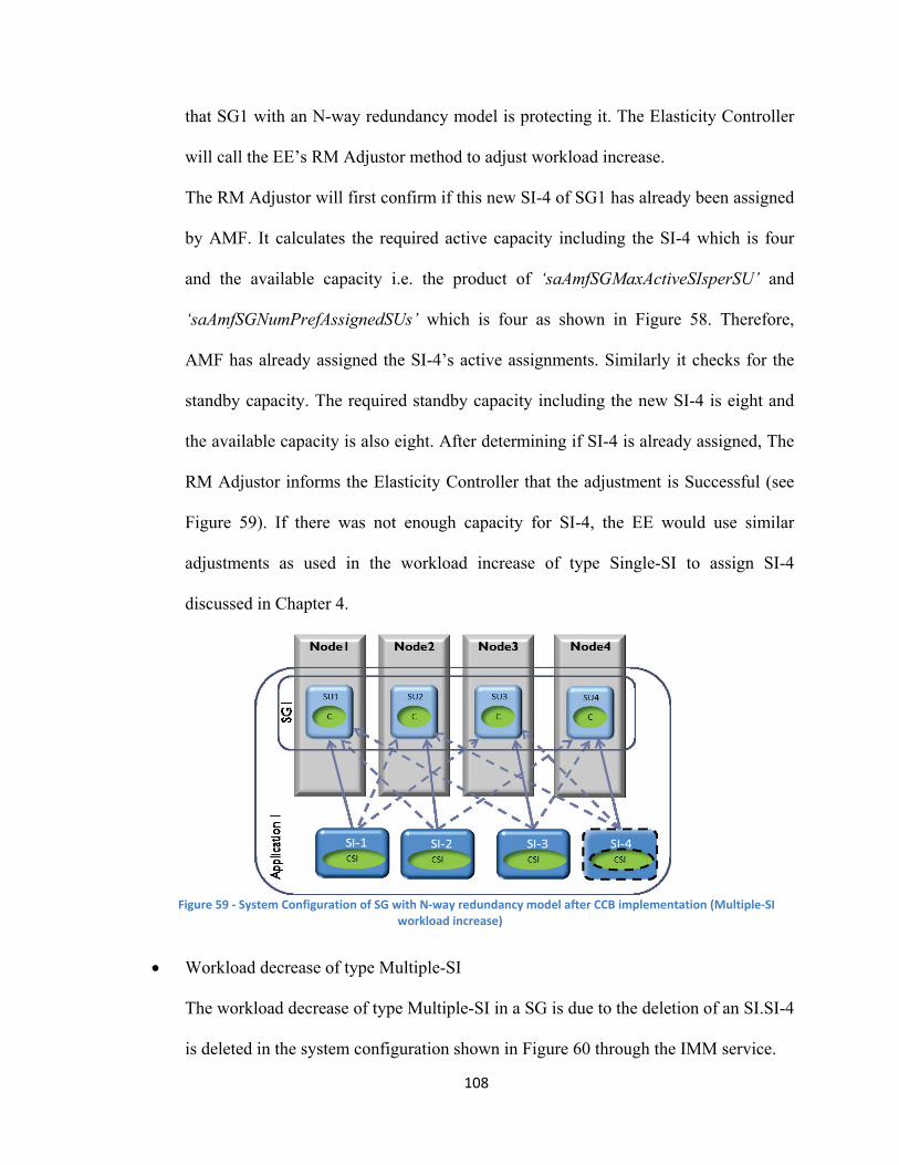
that SG1 with an N-way redundancy model is protecting it. The Elasticity Controller

will call the EE’s RM Adjustor method to adjust workload increase.

The RM Adjustor will first confirm if this new SI-4 of SG1 has already been assigned

by AMF. It calculates the required active capacity including the SI-4 which is four

and the available capacity i.e. the product of ‘saAmfSGMaxActiveSIsperSU’ and

‘saAmfSGNumPrefAssignedSUs’ which is four as shown in Figure 58. Therefore,

AMF has already assigned the SI-4’s active assignments. Similarly it checks for the

standby capacity. The required standby capacity including the new SI-4 is eight and

the available capacity is also eight. After determining if SI-4 is already assigned, The

RM Adjustor informs the Elasticity Controller that the adjustment is Successful (see

Figure 59). If there was not enough capacity for SI-4, the EE would use similar

adjustments as used in the workload increase of type Single-SI to assign SI-4

discussed in Chapter 4.

Figure 59 - System Configuration of SG with N-way redundancy model after CCB implementation (Multiple-SI

workload increase)

• Workload decrease of type Multiple-SI

The workload decrease of type Multiple-SI in a SG is due to the deletion of an SI.SI-4

is deleted in the system configuration shown in Figure 60 through the IMM service.

108

Configuration:

Attribute Names SG1


Ordered List of SIs {SI-1, SI-2, SI-3, SI-4}







Figure 60 - System Configuration of SG with N-way redundancy model before CCB implementation (Multiple-SI

workload decrease)

When the EE’s Elasticity Controller gets a callback from the IMM service informing

the deletion of SI-4, it determines that the workload decrease is in SG1 with an N-

way-Active redundancy model. It calls the RM Adjustor to adjust the workload

decrease.

The RM Adjustor method uses ‘Re-grouping the SIs on less SUs of the SG’ strategy

explained in Chapter 4.The RM Adjustor checks three conditions before decreasing

109

the number of assigned SUs. It checks to see if the number of SUs left after

subtracting the SUs that it plans to decrease is enough for the SIs protected by the SG.

The RM Adjustor checks to see if the value ‘saAmfSGNumPrefAssignedSUs-1’ of SG

is greater than or equal to ‘saAmfSIPrefStandbyAssignments’ plus one of each SI

protected by SG. For the system configuration shown in Figure 60, the number of

SUs is three after decreasing the number of assigned SUs in SG which is greater than

each of the SI’s number of standby assignments plus one. The RM Adjustor checks if

the active capacity is enough for the SIs by comparing the number of SIs protected by

SG with the product of the values of ‘saAmfSGMaxActiveSIsperSU’ and

‘saAmfSGNumPrefAssignedSUs-1’ attributes of SG. For the system configuration

shown in Figure 60, the active capacity is three. After confirming that the active and

standby capacity is enough for the SI assignments the RM Adjustor creates a CCB to

decrease the number of assigned SUs and calls the buffer manager.

CCB: saAmfSGNumPrefAssignedSUs: 3

Figure 61 – System Configuration of SG with the N-way redundancy model after CCB implementation (Multiple-SI

workload decrease)

We have presented the EE’s actions for a SG with the 2N and N-way redundancy models

for workload increase and decrease scenarios in the Appendix. The No-Redundancy redundancy

model is similar to the 2N redundancy model except that the EE does not consider standby

110

assignments while handling elasticity. The workload change scenarios for a SG with N+M

redundancy and the N-way-Active redundancy model are previously illustrated in Chapter 5,

thus after the investigations we can conclude the following:

Table 3 - Investigation Scenarios

A check mark denotes that an elasticity action is possible in the particular scenario and

cross mark denotes that the elasticity action is not considered, since the redundancy model is not

very flexible in the scenario.

111

managing high-availability and elasticity in a cluster ... · managing high-availability and...

Documents