managing uncertainties in hardware-software codesign projects

Managing Uncertainties in

Hardware-Software Codesign Projects

Jones Albuquerque (DEINFO-UFRPE)

Ferrer-Savall, J. (ESAB-UPC)

Bocanegra, S. (DEINFO-UFRPE)

Ferreira, T. (DEINFO-UFRPE)

Lopez-Codina, D. (ESAB-UPC)

Coelho Jr, C. (DCC-UFMG)

[email protected]

July 17, 2014

JOA

Resaltado

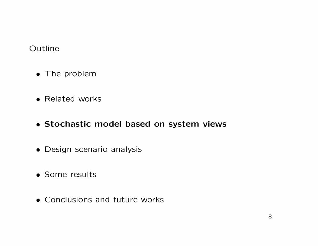
Outline

• The problem

• Related works

• Stochastic model based on system views

• Design scenario analysis

• Some results

• Conclusions and future works

1

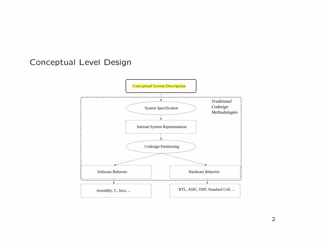
Conceptual Level Design

Conceptual System Description

System Specification

Internal System Representation

Codesign Partitioning

Software Behavior Hardware Behavior

RTL, ASIC, DSP, Standard Cell, ...Assembly, C, Java, ...

Traditional

MethodologiesCodesign

2

JOA

Resaltado

Design Space

DESIGNTOOLS

TARGET

DESIGN

SPACE

general−purpose

DSP system

C

C++

JAVA

TECHNOLOGIES

core−basic ASIC

Standard cell

Assembly

Multiprocessor

FPGA

Min cut

Simulated Annealing

manual partitioningILP

Scheduling Blocks

Formal verification

CONSTRAINTSOPTIMIZATIONCost

AreaPower Development time

Reuse

Latency

Re−programability

Technologies + Constraints + Tools

3

Team Space

DESIGNTOOLS

TARGET

DESIGN

SPACE

general−purpose

DSP system

C

C++

JAVA

TECHNOLOGIES

core−basic ASIC

Standard cell

Assembly

Multiprocessor

FPGA

Min cut

Simulated Annealing

manual partitioningILP

Scheduling Blocks

Formal verification

CONSTRAINTSOPTIMIZATIONCost

AreaPower Development time

Reuse

Latency

Re−programability

TEAMSDevelopment risk

Changes in teams

Task assignment

Team load

Design times

Group communication

Skills

Technologies + Constraints + Tools + TEAMS

4

JOA

Resaltado

JOA

Resaltado

JOA

Resaltado

The Problem

Analysis + Partitioning

Conceptual Design

Task Assignment Task Implementation

Team Technology Technology Implementation

(HW/SW Codesign)(Team Assignment)

5

Related Works/Tools

• Castle, Chinook, COMET, Cosmos, COSYMA, CoWare, LY-COS, Polis, PISH, Ptolemy, Symphony, Vulcan

• COSYMA, Chinook, and LYCOS present estimated analysisand quality profiles

• PISH makes formal verification of the synthesis process

• CASTLE considers teams as designers

• COMET does not require a functionally complete descriptionin its specification

6

Neglected Aspects

• System is implemented by teams detaining specific technolo-

gies

• No single person has a complete knowledge of the system

• Early design scenarios and risk analysis

• Team load and task assignment

• Process is not adjusted neither tuned during development

7

• IEEE/ACM CODES, group discussion:

”This part of system design is very guru-intense and

tool support is scarse”

JOA

Resaltado

Outline

• The problem

• Related works



• Some results


8

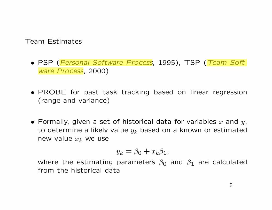
Team Estimates

• PSP (Personal Software Process, 1995), TSP (Team Soft-ware Process, 2000)

• PROBE for past task tracking based on linear regression(range and variance)

• Formally, given a set of historical data for variables x and y,to determine a likely value yk based on a known or estimatednew value xk we use

yk = β0 + xkβ1,

where the estimating parameters β0 and β1 are calculatedfrom the historical data

9

JOA

Resaltado

JOA

Resaltado

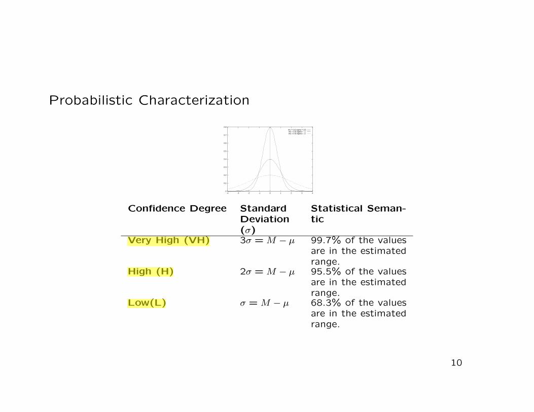
Probabilistic Characterization

0

0.1

0.2

0.3

0.4

0.5

0.6

0.7

0.8

-4 -3 -2 -1 0 1 2 3 4

mu = 0 & sigma = 2/3mu = 0 & sigma = 1 mu = 0 & sigma = 2

Confidence Degree StandardDeviation(σ)

Statistical Seman-tic

Very High (VH) 3σ = M − µ 99.7% of the valuesare in the estimatedrange.

High (H) 2σ = M − µ 95.5% of the valuesare in the estimatedrange.

Low(L) σ = M − µ 68.3% of the valuesare in the estimatedrange.

10

JOA

Resaltado

JOA

Resaltado

JOA

Resaltado

System Described by Views

• Hierarchical view: static objects and dependencies

• Sequencing view: dynamic constraints

• Development view: development dependencies

11

Network Controller

Host CPU

Memory

DMA-RCVD

RCVD-FRAME RCVD-BUFFER RCVD-BIT

DMA-XMIT XMIT-FRAME XMIT-BIT

ENQUEUE EXEC-UNIT

RXE

RXD

TXE

TXD

Execution Unit

Transmit Unit

Receive Unit

Bus Unit

Hierarchical View

12

Hierarchical Graph

Net Controller

Bus_Unit Receive_ Unit

Transmit_ Unit

Execution_ Unit

DMA-RCVD RCVD-FRAME

RCVD-BUFFER RCVD-BIT

DMA-XMIT XMIT-FRAME

XMIT-BIT

ENQUEUE

EXEC-UNIT

13

Sequencing View

RCVD_BIT:RXData

RCVD_BUFFER:RXByte

RCVD_FRAME:RxFrame

RCVD_DMA:DMA_write

<1us

BUS UNIT:bus_dma_write

14

Sequencing Graph

initial_method

final_method

rcvd_bit

rcvd_buffer

rcvd_frame

dma_rcvd

bus_dma_write

bus_dma_read

dma_xmit

xmit_frame

xmit_bit

bus_read/write

enqueue

exec_unit

< 1us < 1.2us< 5us

0 us

0 us

0.1us

0.1us

0.4us

0.4us

0.1us

0.3us

0.8us

2us

3us

15

Development View

Host CPU

Memory

DMA-RCVD

RCVD-FRAME RCVD-BUFFER RCVD-BIT

DMA-XMIT XMIT-FRAME XMIT-BIT

ENQUEUE EXEC-UNIT

RXE

RXD

TXE

TXD

Execution Unit

Transmit Unit

Receive Unit

Bus Unit

16

Development Graph

RCVD-

BIT

RCVD-

BUFFER

RCVD-

FRAME

RCVD-

DMA

DMA-

XMIT

XMIT-

FRAME

XMIT

BIT

ENQUEUE

EXEC-UNIT

BUS-UNIT

INITIAL-OBJECT

FINAL-OBJECT

8 weeks

7 weeks

9 weeks

10 weeks

0 weeks0 weeks

2 weeks 3 weeks 3 weeks

3 weeks 4 weeks

Receive Unit

Transmit_Unit

Execution_Unit

17

The Design Process using System Views

1. The system is described as a collection of interconnected objects (hierarchicalview) in compliance with system’s functional specification;

2. The sequential and development views of the system are determined by the projectmanager;

3. The main constraints of the system design are determined and annotated intheir respective views;

4. The system-level model is given to the development teams;

5. The development teams estimate values for each object and method consideringthe technology options and the team’s skill;

6. For each design scenario:The automatic tool will choose the best implementation con-sidering theobjective function, that must be optimized (cost function), andthe riskof success for satisfying the design constraints (inference de-grees).

18

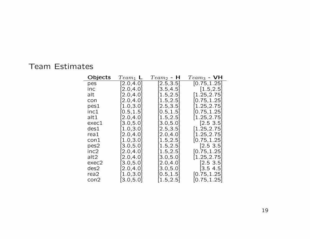
Team EstimatesObjects Team1 L Team2 - H Team3 - VHpes [2.0,4.0] [2.5,3.5] [0.75,1.25]inc [2.0,4.0] [3.5,4.5] [1.5,2.5]alt [2.0,4.0] [1.5,2.5] [1.25,2.75]con [2.0,4.0] [1.5,2.5] [0.75,1.25]pes1 [1.0,3.0] [2.5,3.5] [1.25,2.75]inc1 [0.5,1.5] [0.5,1.5] [0.75,1.25]alt1 [2.0,4.0] [1.5,2.5] [1.25,2.75]exec1 [3.0,5.0] [3.0,5.0] [2.5 3.5]des1 [1.0,3.0] [2.5,3.5] [1.25,2.75]rea1 [2.0,4.0] [2.0,4.0] [1.25,2.75]con1 [1.0,3.0] [1.5,2.5] [0.75,1.25]pes2 [3.0,5.0] [1.5,2.5] [2.5 3.5]inc2 [2.0,4.0] [1.5,2.5] [0.75,1.25]alt2 [2.0,4.0] [3.0,5.0] [1.25,2.75]exec2 [3.0,5.0] [2.0,4.0] [2.5 3.5]des2 [2.0,4.0] [3.0,5.0] [3.5 4.5]rea2 [1.0,3.0] [0.5,1.5] [0.75,1.25]con2 [3.0,5.0] [1.5,2.5] [0.75,1.25]

19

Design Scenarios

• Early design options

• Risk analysis without implementation costs

• Time-to-market

• Implementation cost

• Execution time

• Team load

Mathematical model incorporating system views, team estimates, and risk analysis

20

Mathematical Formulation

SILP - Stochastic Integer Linear Problem

min{∑i,j

cijxij}

s.t.

Prob{∑

j

aijxij ≤ bi} ≥ 1− αi,

where xij ∈ {0,1}, aij, bi and cij are random variables, and 0 ≤ αi ≤ 1 represents the

uncertainty that the equation will be satisfied.

21

Constraints: only one initial/final week

• There is only one initial (γijk) and final (Γijk) week for each

object i implemented by team j, i.e.

∀i ∈ Objects, j ∈ Teams∑

k∈Weeks

γijk = xij;

∀i ∈ Objects, j ∈ Teams∑

k∈Weeks

Γijk = xij.

22

Constraints: path execution time

• Path execution time. For each path (p) in SG Graph (se-

quencing view), the estimated execution time of the meth-

ods implemented by teams (dmj) in the path must satisfy a

maximum execution time (DIp) with a defined probability of

certainty (1 − αpath). Each method m of object i in path

p ∈ PathsE is represented by a 3-tuple (i, p,m), i.e.

∀P ∈ PathsE, j ∈ Teams

Prob{∑

(i,p,m)∈Pdmjxij ≤ DIp} ≥ 1− αpath

23

Constraints: team load

• Maximum load for team j (k1 is the first week). At week k1: team j can be implementingan object i or not, i.e.

∀i ∈ Objects, j ∈ Teams aijk1 = γijk1 − Γijk1

where, ∀ijΓijk1 = 0. At other weeks: team j can be implementing object i if it beginsin this week (γijk = 1) or it is already implementing it (aij(k−1) = 1) and it did not endyet (Γijk = 0), i.e.

∀i ∈ Objects, j ∈ Teams, k ∈ Weeks aijk = aij(k−1) + γijk − Γijk

At each week, the maximum load of a team (Λj) must be satisfied, i.e. the entire effortwasted on all objects by a team at a week must be less or equal to the maximum loadof this team with a defined probability of certainty (1− αload). Thus,

∀j ∈ Teams, k ∈ Weeks Prob{∑

i∈Objects

λijaijk ≤ Λj} ≥ 1− αload

24

Constraints: object assignment

• Object assignment. The final week (Γijk) of an implemen-

tation is greater or equal the development time (tij) plus

the initial week (γijk) with a defined probability of certainty

(1− αassignment), i.e.

∀i ∈ Objects, j ∈ Teams

Prob{∑

k∈Weeks

kΓijk ≥ tijxij +

∑k∈Weeks

kγijk} ≥ 1− αassignment.

25

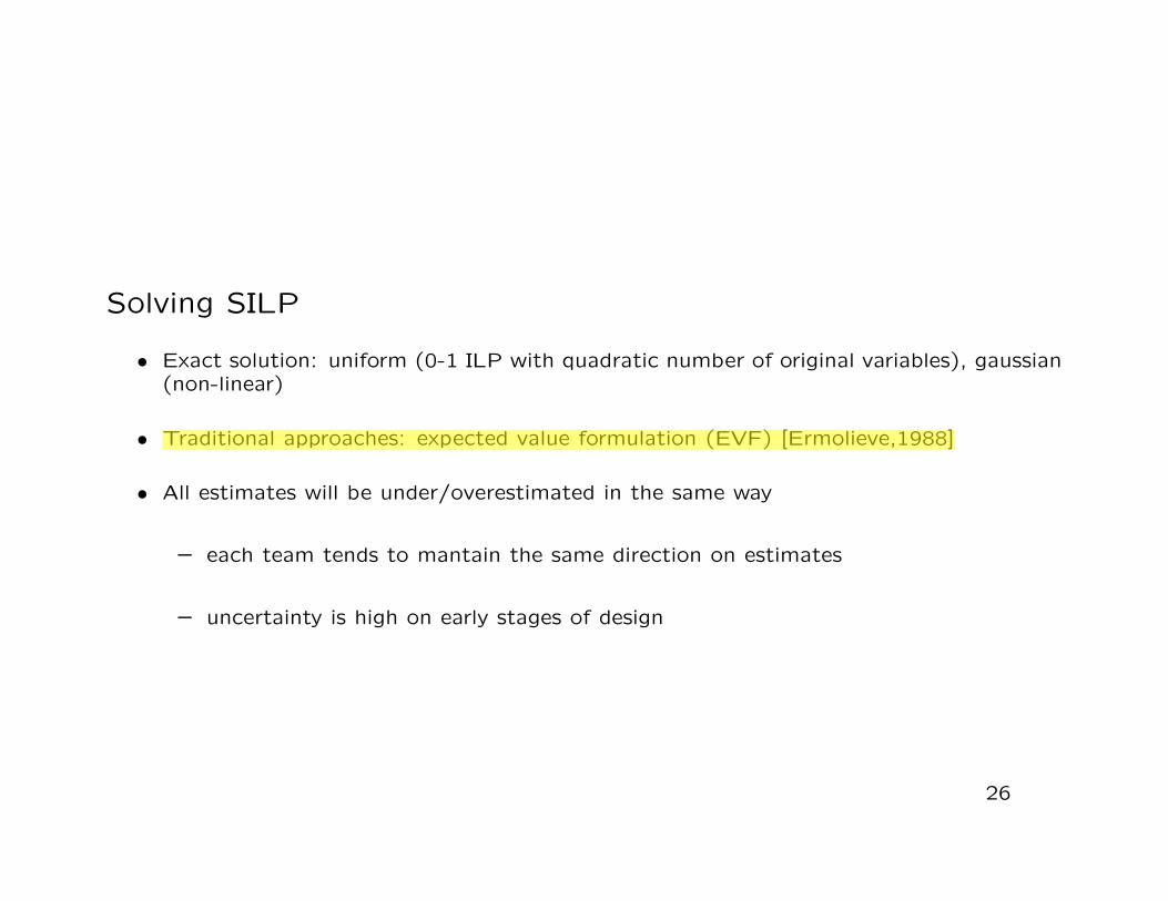
Solving SILP

• Exact solution: uniform (0-1 ILP with quadratic number of original variables), gaussian(non-linear)

• Traditional approaches: expected value formulation (EVF) [Ermolieve,1988]

• All estimates will be under/overestimated in the same way

– each team tends to mantain the same direction on estimates

– uncertainty is high on early stages of design

26

JOA

Resaltado

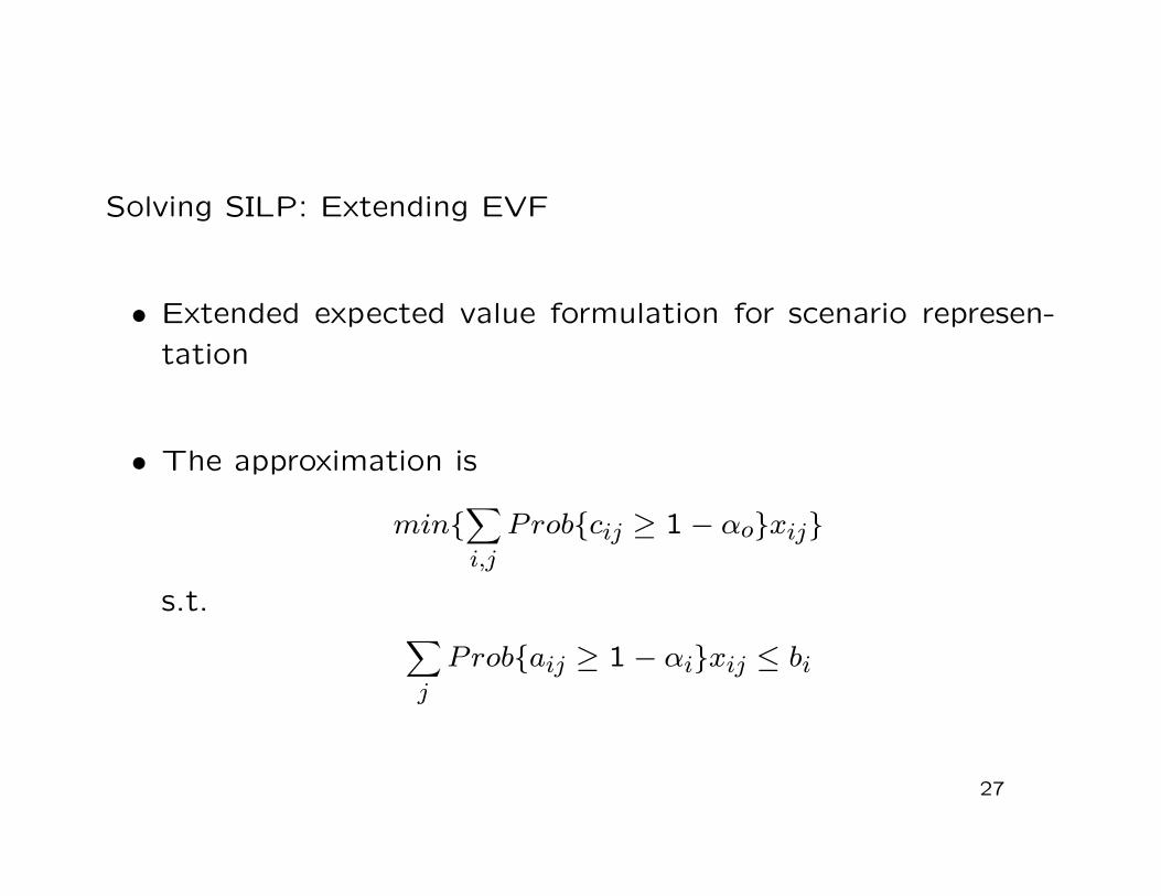
Solving SILP: Extending EVF

• Extended expected value formulation for scenario represen-

tation

• The approximation is

min{∑i,j

Prob{cij ≥ 1− αo}xij}

s.t. ∑j

Prob{aij ≥ 1− αi}xij ≤ bi

27

Scenario Representation

aij = (µaij + F−1(1− αi)σaij),

where F−1(1− αi) is the inverse CDF for Gaussian distribution:

1− α = 50% → F−1(1− αi) = 01− α = 80% → F−1(1− αi) = 11− α = 97% → F−1(1− αi) = 21− α = 99% → F−1(1− αi) = 3

50% 80% 99% x

F(x)

F(x) = CDF of continuos random variable

28

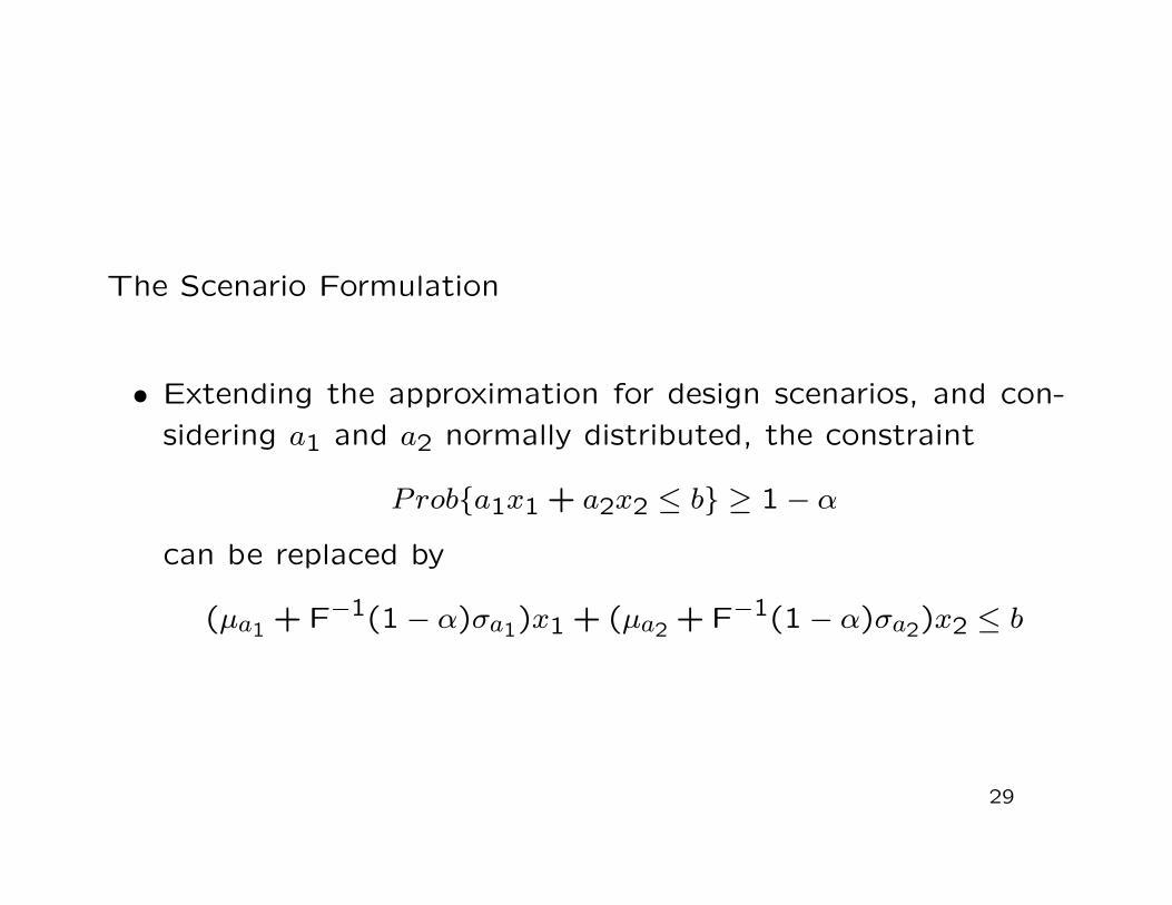
The Scenario Formulation

• Extending the approximation for design scenarios, and con-

sidering a1 and a2 normally distributed, the constraint

Prob{a1x1 + a2x2 ≤ b} ≥ 1− α

can be replaced by

(µa1 +F−1(1− α)σa1)x1 + (µa2 +F−1(1− α)σa2)x2 ≤ b

29

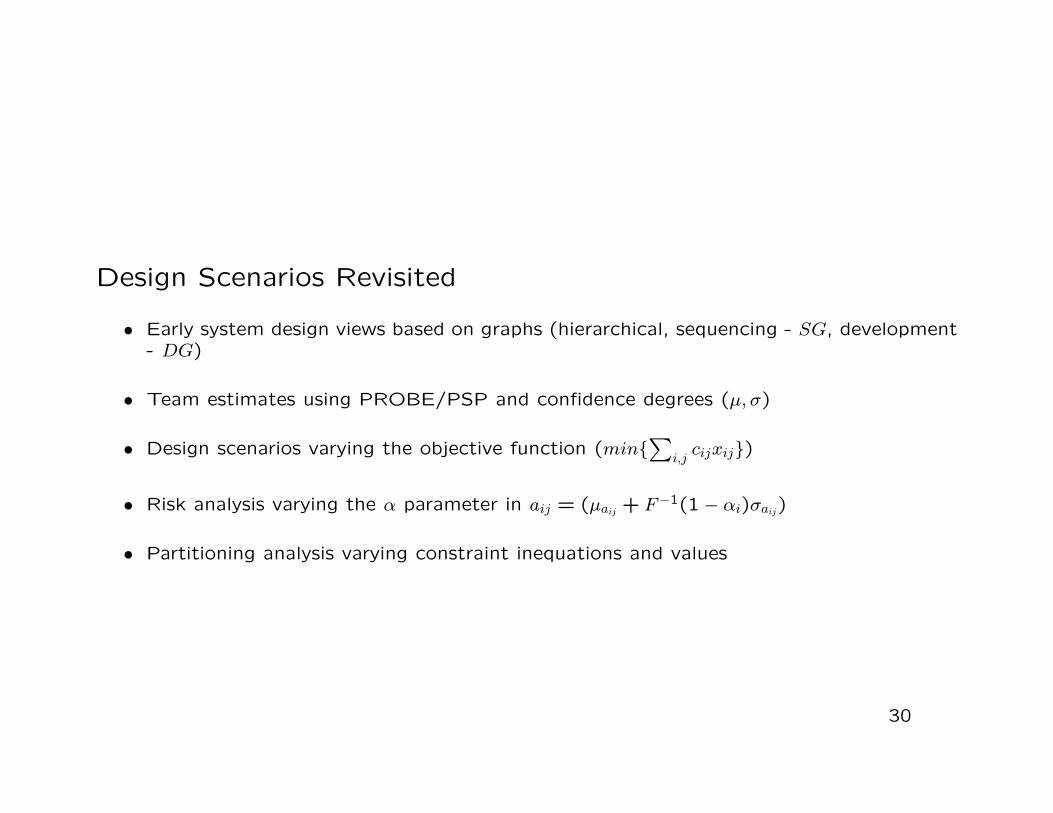
Design Scenarios Revisited

• Early system design views based on graphs (hierarchical, sequencing - SG, development- DG)

• Team estimates using PROBE/PSP and confidence degrees (µ, σ)

• Design scenarios varying the objective function (min{∑

i,jcijxij})

• Risk analysis varying the α parameter in aij = (µaij + F−1(1− αi)σaij)

• Partitioning analysis varying constraint inequations and values

30

Outline

• The problem

• Related works



• Some results


31

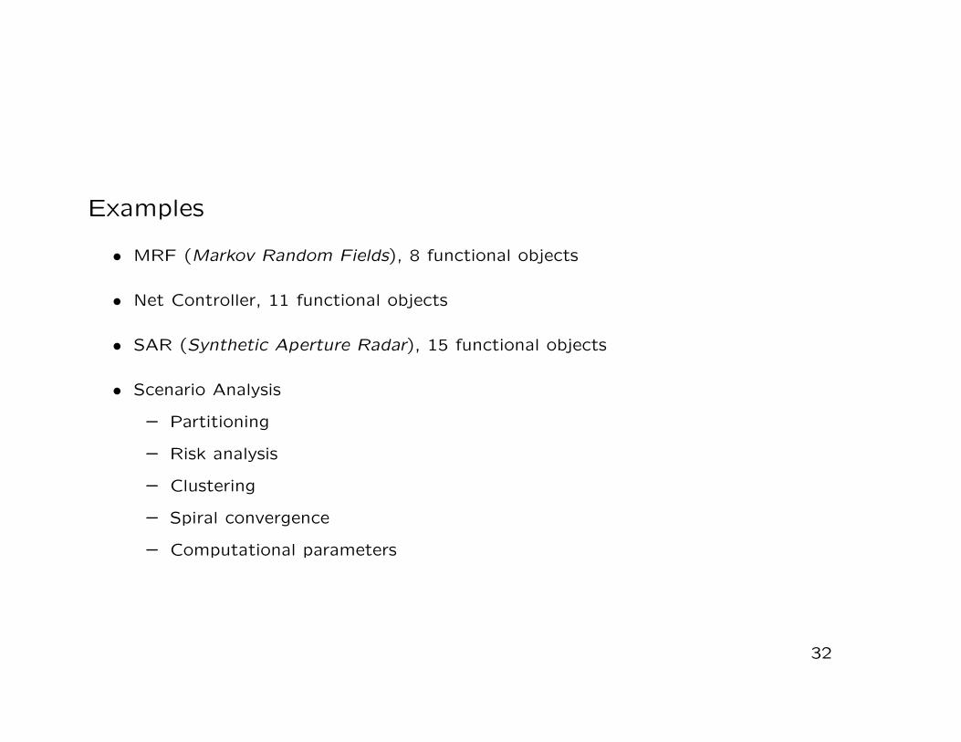
Examples

• MRF (Markov Random Fields), 8 functional objects

• Net Controller, 11 functional objects

• SAR (Synthetic Aperture Radar), 15 functional objects

• Scenario Analysis

– Partitioning

– Risk analysis

– Clustering

– Spiral convergence

– Computational parameters

32

Partitioning Analysis

33

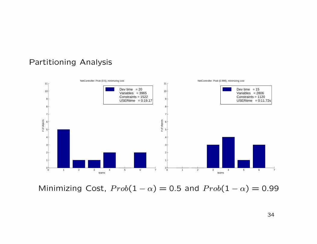
Partitioning Analysis

0 1 2 3 4 5 6 70

1

2

3

4

5

6

7

8

9

10

11NetController: Prob (0.5), minimizing cost

teams

# of

obj

ects

Dev time = 20Variables = 3965Constraints = 1522USERtime = 0:19.17

0 1 2 3 4 5 6 70

1

2

3

4

5

6

7

8

9

10

11NetController: Prob (0.999), minimizing cost

teams

# of

obj

ects

Dev time = 15Variables = 2806Constraints = 1120USERtime = 0:11.72s

Minimizing Cost, Prob(1− α) = 0.5 and Prob(1− α) = 0.99

34

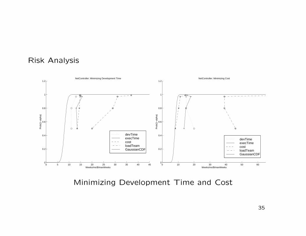
Risk Analysis

0 5 10 15 20 25 30 35 40 450

0.2

0.4

0.6

0.8

1

1.2NetController: Minimizing Development Time

Weeks/ms/$/manWeeks

Pro

b(1−

alph

a)

devTimeexecTimecostloadTeamGaussianCDF

0 10 20 30 40 50 600

0.2

0.4

0.6

0.8

1

1.2NetController: Minimizing Cost

Weeks/ms/$/manWeeks

Pro

b(1−

alph

a)


Minimizing Development Time and Cost

35

Risk Analysis

0 10 20 30 40 50 600

0.2

0.4

0.6

0.8

1

1.2NetController: Minimizing Execution Time

Weeks/ms/$/manWeeks

Pro

b(1−

alph

a)


0 10 20 30 40 50 600

0.2

0.4

0.6

0.8

1

1.2NetController: Minimizing Team Load

Weeks/ms/$/manWeeks

Pro

b(1−

alph

a)


Minimizing Execution Time and Team Load

36

Clustering

Risk NetWork Controller - Objects (min Dev Time)rcvd xmit enqueue exec bit buffer frame xmit b xmit f

0.5 tm1 tm1 tm1 tm1 tm1 tm2 tm3 tm4 tm40.8 tm3 tm3 tm3 tm3 tm3 tm6 tm3 tm4 tm40.97 tm3 tm3 tm3 tm3 tm3 tm5 tm3 tm4 tm40.99 tm6 tm3 tm3 tm4 tm3 tm4 tm4 tm4 tm4

Clustering team assignment when minimizing System Cost

37

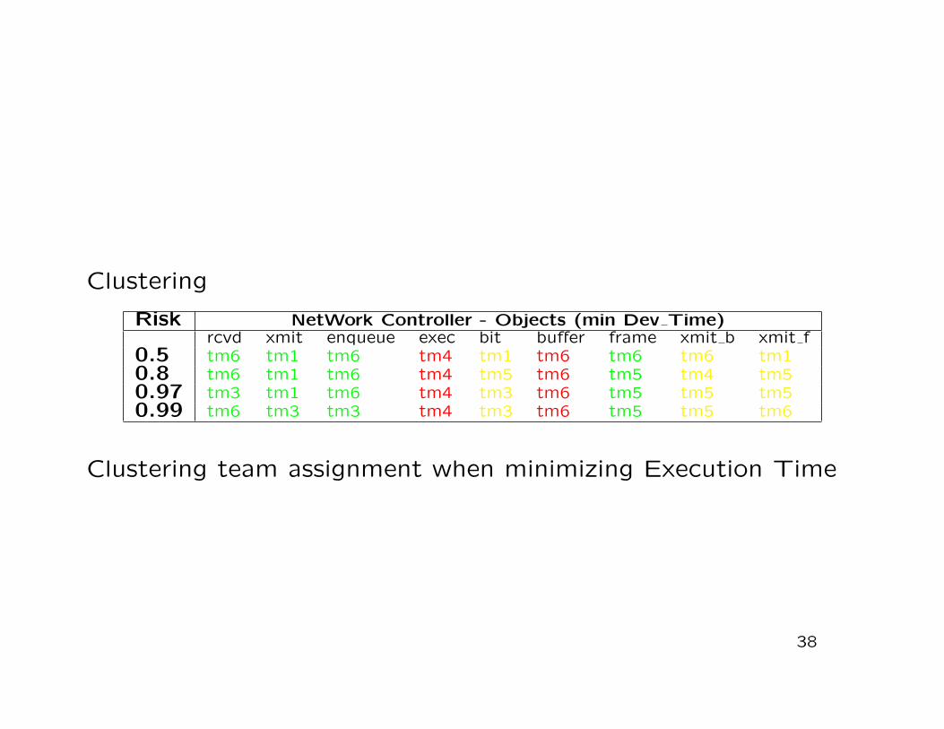
Clustering

Risk NetWork Controller - Objects (min Dev Time)rcvd xmit enqueue exec bit buffer frame xmit b xmit f

0.5 tm6 tm1 tm6 tm4 tm1 tm6 tm6 tm6 tm10.8 tm6 tm1 tm6 tm4 tm5 tm6 tm5 tm4 tm50.97 tm3 tm1 tm6 tm4 tm3 tm6 tm5 tm5 tm50.99 tm6 tm3 tm3 tm4 tm3 tm6 tm5 tm5 tm6

Clustering team assignment when minimizing Execution Time

38

Convergence Analysis

1 2 6 9 11 i

P(i)

i

P(i)

2 2 3 4 1195

Minimizing Development Time and Execution Time

39

Computational Parameters

Times for first iteration

Case-Study Num.variables Num.constraints Iterations USER Time (h:m:s)MRF 2852 1089 13890 00:01:02NET 3965 1462 38576 00:03:32SAR 7260 2690 187808 01:16:21

Constraints = O(objects× weeks× teams)

40

Conclusions

• A stochastic model to system design by teams and multiple

technologies on conceptual level

• Interactive partitioning using design manager decisions based

on clustering scenarios

• Clustering scenarios to refine the process and minimize the

SILP problem at each iteration, reducing the computational

time

41

Contributions

• A stochastic model for system design by teams

• An approach with confidence degrees to model risk analysis and team aspects

• System description by views on early stages (conceptual level design)

• A mathematical formulation for partitioning with multiple technologies

• An extended expected value formulation to represent design scenarios

• Interactive and iterative partitioning using clustering to refine the process and to reducethe SILP problem

• Design scenarios representing partitioning options, uncertainty, team aspects and designconstraints

42

At Work

• Applying in real industry: PINTO FILHO, K. V. ; BOCANEGRA, S. ; ALBUQUERQUE,J. . Uma proposta de modelagem para o calculo de reservas de contingencia e gerencialem projetos de software usando programacao linear inteira estocastica DOI 10.5752/P.2316-9451.2012v1n1p50. Abakos, v. 1, p. 50-74, 2012.

• Integrating conceptual level design in a commercial tool (FACEPE - 2013-2015)

• Solving SILP: other approximations, Interior Points, and parallel strategies

• Other mathematical formulations for the conceptual level design problem and heuristics

43

JOA

Resaltado

JOA

Resaltado

Aknowledgements

• This work was [partially] supported by the National Insti-

tute of Science and Technology for Software Engineering

(www.ines.org.br), funded by CNPq and FACEPE, grants

573964/2008-4 and APQ-1037-1.03/08.

44