1

Manifestations of Capital-Theoretic ‘Paradoxes’ in Temporary Equilibria

Robert L. Vienneau, Independent Researcher January 2006

Abstract: Only Sections 2, 3, and 4 are complete. I need to write Section 5 before writing this abstract and completing Sections 6 and Section 1. The issues here:

1. The Sraffians showed traditional long-period neoclassical models, which take the quantity of capital as given in some sense or another, are incorrect.

2. Inasmuch as the pre-analytical vision of prices as scarcity indices and the principle of substitution are central to neoclassical economics, the theory is still incorrect. The transition to short-run models of intertemporal and temporary equilibrium does not change this result.

3. These neoclassical short-run models, insofar as they take the initial quantities of capital goods as data, cannot allow for any time to reach equilibrium. Such time would change the data and thus make the initially determined equilibrium path irrelevant.

a. Nevertheless, can Cambridge models tell us something about those paths? b. Can Cambridge models tell us something about disequiliibrium

tatonnement processes to reach those paths? c. The demonstration that long period prices are not scarcity indices takes in

more than the possibility of the existence of switch points with reverse capital deepening. If the answer to the above two questions is in the affirmative, does either answer rely more on the structure of long period prices at non-switching points and non-perverse switch points than on perverse switch points?

4. Can the theory of long period positions tell us something about actual economies without a short period dynamics to back it up?

5. If not, what is a short period dynamic model that can be set in historical time? 6. How, otherwise can long period production models be closed, other than with

intertemporal utility-maximizing? 7. The answers to Questions 1, 2, 3, and 5 seem to be a matter of logic and

mathematical modeling. The answer to Question 4 and the usefulness of the answers to Questions 5 and 6 seem to require empirical support.

This paper concentrates on the answers to Questions 2 and 3. Keywords: B51: Sraffian Economics, C61: Dynamic Analysis, C67: Input-Output

Models, D33: Factor Income Distribution, D57: Input-Output Analysis, D90: Intertemporal Choice, E22: Capital Theory.

2

1.0 Introduction The Cambridge Capital Controversy (CCC) is a long-lasting, complex, and multifaceted affair.1 Critics associated with Cambridge, UK, attack the logical coherence of neoclassical theory and claim to outline an alternative approach to economics.2 The Cambridge critics show examples of apparently paradoxical behavior, most notably reswitching and capital-reversing, within optimizing models. Neoclassical economists argue that the most rigorous versions of neoclassical theory, short run models of General Equilbrium theory, are unaffected by Cambridge criticism. This paper provides an overview of these arguments, thereby introducing the reader to ongoing contemporary debates. The Sraffians, taking neoclassical theory as they found it, showed the theory to be mistaken. The most prominent neoclassical economists responding to the CCC acknowledge that many models in the mainstream literature are problematic in theory. Austrian capital theory, Clarkian capital theory, and Solovian growth theory are among the approaches recognized to be theoretically questionable.3 In a comparison of long period equilibrium positions, greater capital intensity need not be associated with a lower interest rate. Nor is greater sustainable consumption per head necessarily associated with a lower interest rate. The interest rate is generally not equal in equilibrium to the marginal product of capital4. Neoclassical economists5 argue, however, the canonical neoclassical theory is best expressed in disaggregated short period General Equilibrium models of intertemporal6 and temporary equilibria.7 They claim belief in the logical consistency and coherence of these models is and should be unaffected by Cambridge criticism. In fact, inasmuch as reswitching and reverse capital deepening are analyzed within a neoclassical framework, these phenomena are implications of neoclassical theory.8 Some of these

1 Cohen and Harcourt (2003) provide a recent survey. Some letters in the Fall 2003 issue of the Journal of Economic Perspectives comment on that article. 2 The constructive aspects of Sraffian economics fall outside the scope of this paper. In particular, neither the relationship between Sraffa’s work and Classical and Marxian economics (see, for example, Garegnani 1984 and 1990a) nor the compatibility of Sraffian economics and the economics of Keynes are discussed here. 3 Samuelson 1966 and 2001. 4 Harcourt (1969). 5 Bliss 1975, Burmeister 1980, Dixit 1977, Hahn 1982, Samuelson 1975, and Stiglitz 1974. 6 Debreu 1959. 7 Burmeister 1980, Grandmont 1977, Hicks 1946. 8 Mas-Colell 1989, Solow 1975.

3

economists suggest that Cambridge findings might have implications for stability analysis.9, 10 The turn towards short period General Equilibrium models has not gone unchallenged by partisans of Cambridge criticism. Need to discuss those who argue neoclassical dynamic models cannot tell us anything about actual economies Papers by those sympathetic to Sraffians arguing Cambridge paradoxes have implications for dynamics: Dumenil, G. and Levy D. (1985). “The Classicals and the Neoclassicals: A Rejoinder to Frank Hahn”, Cambridge Journal of Economics, V. 9: 327-345. Garegnani, P. (2000). “Savings, Investment, and Capital in a System of General Intertemporal Equilibrium”, in Critical Essays on Piero Sraffa’s Legacy in Economics (edited by H. D. Kurz), Cambridge: Cambridge University Press. Garegnani, P. (2003). “Capital and Intertemporal Equilibrium: A Reply to Mandler”, Mimeo. (I haven’t actually seen this yet.) Rosser, J. B., Jr. (1983). “Reswitching as a Cusp Catastrophe”, Journal of Economic Theory, V. 31, N. 1: 182-193. Rosser, J. B., Jr. (1991). From Catastrophe to Chaos: A General Theory of Economic Discontinuities, Boston: Kluwer. (What about 2nd edition?) Schefold, B. (1997). “Classical Theory and Intertemporal Equilibrium”, in Normal Prices, Technical Change, and Accumulation, New York: St. Martin’s Press. Schefold, B. (2000) Schefold, B. (2003?). “Reswitching as a Cause of Instability of Intertemporal Equilibrium”, Metroeconomica, July? Recent papers on the other side: Bloise and Richlin (2005)

9 “In such instances of multiple rest points, the point toward which the optimizing economy converges depends crucially upon the initial capital-stock conditions. Therefore, the dynamics of the problem become very complex… Such conditions do not arise in regular economies [that is, economies without capital-reversing. The assumption of no capital-reversing] is sufficient for the uniqueness of the rest-point solution…” (Burmeister 1980). 10 “Such a theory concerns an economy in full neoclassical equilibrium which, I have repeatedly argued, has nothing to fear from anything in Sraffa’s or in his followers’ work. But on the manner in which such an equilibrium is supposed to come about, neoclassical theory is highly unsatisfactory. Sraffa’s work shows that certain simplified routes are very risky and not free from logical difficulties. The remarkable fact is that neither he nor the Sraffians have made anything of this” (Hahn 1982).

4

Ferretti (2004) Mandler, M. (1999). Dilemmas in Economic Theory, Oxford: Oxford Unversity Press. Mandler, M. (2002). “Classical and Neoclassical Indeterminacy in One-Shot vs. Ongoing Equilibria”, Metroeconomica, V. 53, N. 3: 203-222. Mandler, M. (2004). “Well-Behaved Production Economies”, January. Where does Mas-Colell (1989) fit? How about Marglin (1984). Section 2 sets out a model of dynamic equilibrium paths. Section 3 develops a model of limit points of the dynamic paths for the model, that is, stationary states. Some examples are put forward. Section 4 points out traditional neoclassical theory cannot be reconciled with the structural stability analysis arising in the Section 3 examples of stationary states. Bifurcations of limit points can arise in reswitching examples as a parameter in the utility function varies. Bifurcations also arise in a non-reswitching, non capital-reversing example. The results suggest that both price and real Wicksell effects can generate paradoxical or counter-intuitive dynamic paths. Section 5 considers implications for neoclassical dynamics of Cambridge models. Considers local stability of stationary states; that is, do nearby dynamic equilibrium path converge to or diverge from a stationary state path. Considers traverses from one stationary state to another across a perverse switch point. Considers tatonnement stability. Section 6 presents some conclusions. List of Symbols Ω(t ) A two-element column vector denoting the quantities of goods a firm possesses

at the start of the (t + 1) st year. δ A parameter in a log-linear intertemporal utility function. γ The stationary state value of the utility function parameter. γ(t ) A parameter in the utility function of the agent born at the start of the tth year. ω1(t ) The tons steel in the firm’s inventory at the start of the (t +1) st year. ω2(t ) The bushels corn in the firm’s inventory at the start of the (t +1) st year. Aη, η =α,β . Leontief input-output matrix for the η technique. The ith, jth element is

the quantity of the ith commodity required as input for unit output in the jth industry.

C(t ) The deviation of bushels corn consumed per worker from the stationary state consumption per worker.

I The identity matrix. I(r ) The stationary-state value, in bushels corn, of gross investment. I( t ) The value, in bushels corn, of gross investment at the end of the tth year.

5

L(t ) The person-years of labor employed during the tth year. P1(t ) The deviation of the price of steel from the stationary state price of steel. Q(t ) The deviation of gross outputs of steel and corn from stationary state gross

outputs. R( t ) The deviation of the rate of profits from the stationary state rate of profits. S(r ) The stationary-state value, in bushels corn of gross savings. S( t ) The value, in bushels corn, of gross savings out of the output available at the

end of the tth year. U c0(t ),c1(t );γ( t )[ ] The utility function of the agent born at the start of the tth year. W( t ) The deviation of the wage from the stationary state wage. X1

η(t ), η = α,β . The tons of steel produced by a firm with the η process during the tth year. The output of steel is available at the end of the year.

X2 (t ) The bushels corn produced by a firm during the tth year. The output of corn is available at the end of the year.

X3(t ) Value of the firm's unspent endowment in the tth year. a• j

η , j = 1, 2; η =α,β . Two-element column vector comprising the jth column of Aη.

a0η , η =α,β . Two-element row vector of labor coefficients for the η technique. The

jth element is the person-years of labor input for the unit output in the jth industry. e j The jth column of the identity matrix. c , c * Bushels corn consumed at the end of each year in a stationary state. c(t ) Bushels corn consumed at the end of the tth year. c0 (t ) Bushels corn consumed at the end of the tth year by the agent born at the start

of the tth year. c1(t ) Bushels corn consumed at the end of the (t + 1)st year by the agent born at the

start of the tth year. cn Stationary-state bushels corn consumed by agent at the end of the nth year after his

birth. p(r ) A two-element row vector denoting the spot prices of steel and corn quoted on

the market at the end of each year in a stationary state. Since corn is the numeraire, the second element is unity.

p(t ) A two-element row vector denoting the spot prices of steel and corn quoted on the market at the end of the tth year. Since corn is the numeraire, the second element is unity.

p1 * The stationary state spot price of steel. q , q* A two element column vector denoting the quantities of steel and corn

produced and available at the end of each year in a stationary state. q(t ) A two element column vector denoting the quantities of steel and corn produced

and available at the end of the tth year. r , r * The interest rate in a stationary state on a bushel corn borrowed at the start of

the year and paid at the end of the year. Also known as the rate of profits. rmax The maximum stationary-state value of the rate of profits.

6

r(t ) The interest rate on a bushel corn borrowed at the start of the tth year and paid at the end of the tth year. Also known as the rate of profits.

w(r ), w* The wage, in bushels corn, paid at the end of each year in a stationary state for a person-year employed during the year.

w(t ) The wage, in bushels corn, paid at the end of the tth year for a person-year employed during the tth year.

2.0 An Overlapping Generations Model Assume net output, in the numeric example of a very simple temporary equilibrium model, consists of steel, measured in tons, and corn, measured in bushels. Corn is the only consumption good in this economy. Both commodities, steel and corn, can be used as capital goods in producing more steel or corn. Table 1 defines the technology11 available to the firms in this economy. The managers of the firms know of only one process for producing corn, which requires inputs of labor, steel, and corn. Steel can be produced by either one of two processes, and those processes also require inputs of labor, steel, and corn. All production processes require a year to complete, exhibit Constant Returns to Scale (CRS), and totally use up their inputs.12 Outputs of each process become available at the end of the year.

Table 1: Available Production Processes Steel Processes Corn Process Inputs α β Labor 1 Person-Year

3

6481,885

Person-Years 1 Person-Year

Steel

13713,860

Ton

2,1736,300

Ton

37713,860

Ton

Corn

2

17,94737,700

Bushels

7,733188,500

Bushel 11

100 Bushel

Output 1 Ton Steel 1 Ton Steel 1 Bushel Corn A technique is formed by a combination of a steel-producing process and the corn-producing process. Two techniques, alpha and beta, can be constructed from the given technology. Each technique is named for the selected steel-producing process in the technique. Each technique is specified by a row vector representing the labor inputs in the two processes comprising the technique:

a0

α = a01α a02

α[ ]= 1 1[ ] (1)

11 The coefficients of production are defined, as described in Vienneau (2005b), to yield “nice” fractions for stationary-state switch points and the intercepts of the wage-profits curves with the wage axis. 12 So this is a circulating capital model. Furthermore, no joint production is assumed.

7

a0

β = a01β a02

β[ ]=6,3031,885

1⎡

⎣ ⎢ ⎢

⎤

⎦ ⎥ ⎥ (2)

and a 2x2 Leontief matrix containing the remaining coefficients of production:

Aα = a•1α a•2

α[ ]= a11α a12

α

a21α a22

α

⎡

⎣ ⎢ ⎢

⎤

⎦ ⎥ ⎥ =

13713,860

37713,860

93,34737,700

11100

⎡

⎣

⎢ ⎢ ⎢ ⎢ ⎢

⎤

⎦

⎥ ⎥ ⎥ ⎥ ⎥

(3)

Aβ = a•1β a•2

β[ ]=a11

β a12β

a21β a22

β

⎡

⎣ ⎢ ⎢

⎤

⎦ ⎥ ⎥ =

2,1736,300

37713,860

7,733188,500

11100

⎡

⎣

⎢ ⎢ ⎢ ⎢ ⎢

⎤

⎦

⎥ ⎥ ⎥ ⎥ ⎥

(4)

2.1 Production and Prices For what prices will competitive profit-maximizing firms adopt processes consistent with the economy being in a state in which all needed capital goods continue to be (re)produced? An analysis of the firm based on linear programming can answer this question.13 Accordingly, consider a firm that starts the year with an inventory consisting of ω1(t −1) tons steel and ω2(t −1) bushels corn. Let Ω

T (t −1) = ω1(t −1) ω2(t −1)[ ].

The firm faces prices of steel and corn of p(t −1) = p1( t −1) 1[ ] at the beginning of the

year t and prices of steel and corn of p(t ) = p1(t ) 1[ ] at the end of the year.14 Assume that laborers hired to work during the year are paid the wage w(t ) at the end of the year. The managers of the firm set the levels of operation, X1

α (t ) and X1β(t ) , respectively, of

the two steel-producing processes and the level of operation, X2 (t ) , of the corn-producing process to maximize the increment of the value of the firm. They are subject to the constraint that they can purchase the required inputs out of the value of the endowment at the start of the year. Display 5 sets out a Linear Program (LP) specifying the competitive profit-maximizing firm’s problem: Choose X1

α (t ) , X1β(t ) , X2 (t )

To Maximize

p1( t ) −p(t −1) ⋅ a•1η − a01

η w(t )[ ]X1η

η=α,β∑ (t )

+ 1− p( t −1) ⋅ a•2

α − a02α w(t )[ ]X 2(t )

Such That (5)

13 The derivation in this section follows the approach in Vienneau (2005a). 14 Corn is the numeraire throughout this paper.

8

p(t −1) ⋅ a•1η X1

η (t )η=α,β∑ + p(t −1) ⋅ a•2

α X 2(t) ≤ p( t −1) ⋅ Ω(t −1)

X1α (t ) ≥ 0, X1

β(t ) ≥ 0, X2 (t ) ≥ 0 Display 6 specifies the dual LP: Choose r( t ) To Minimize r(t )p(t −1) ⋅ Ω(t −1) Such That (6) p(t −1) ⋅ a•1

η 1+ r (t )[ ]+ a01η w(t ) ≥ p1(t ), η = α, β

p(t −1) ⋅ a•2α 1+ r(t )[ ]+ a02

α w(t ) ≥1 r( t ) ≥ 0 Competition ensures that the corn own-rate of interest minimizes the cost of production. A constraint in the dual LP is met with equality if the corresponding decision variable is positive in the primal LP.

Table 2: Solution of Primal LP Variable in Basis

Value of Basic Variable

When Optimal

X1α (t )

p( t −1) ⋅ Ω(t −1)p(t −1) ⋅ a•1

α

p1(t ) − a01β w( t)

p( t −1) ⋅ a•1β

≤p1(t ) − a01

α w(t )p( t −1) ⋅ a•1

α

1− a02α w(t )

p( t −1) ⋅ a•2α

≤p1(t ) − a01

α w(t )p(t −1) ⋅ a•1

α

p(t −1) ⋅ a•1α + a01

α w(t ) ≤ p1(t )

X1β(t )

p( t −1) ⋅ Ω(t −1)p(t −1) ⋅ a•1

β

p1(t ) − a01α w( t)

p( t −1) ⋅ a•1α

≤p1(t ) − a01

β w(t )p( t −1) ⋅ a•1

β

1− a02α w(t )

p( t −1) ⋅ a•2α

≤p1(t ) − a01

β w(t )p(t −1) ⋅ a•1

β

p(t −1) ⋅ a•1β + a01

β w(t ) ≤ p1(t )

X2 (t )

p( t −1) ⋅ Ω(t −1)p(t −1) ⋅ a•2

α

p1(t ) − a01η w( t)

p( t −1) ⋅ a•1η

≤1− a02

α w(t )p( t −1) ⋅ a•2

α, η =α,β

p(t −1) ⋅ a•2α + a02

α w(t ) ≤1

X3( t ) p(t −1) ⋅ Ω(t −1) p(t −1) ⋅ a•1

η + a01η w(t ) ≥ p1(t ), η = α,β

p(t −1) ⋅ a•2α + a02

α w(t ) ≥1

9

The solution to the primal LP (Table 2) determines which production processes, if any, firms are willing to operate, given any configuration of wages and the price of steel. Consider dynamic paths in which firms find it profitable in each period to continue to produce the capital goods (steel and corn) that are needed to allow the economy to continue. Given the current-year wage and the spot price of steel at the start of the year, one can calculate the spot price of steel along such a path. Likewise, the dual LP shows how to calculate the rate of profits. One still needs to find the initial spot price of steel; the wage; and how much steel and corn is produced each year, given the initial quantities of steel and corn. Only certain ranges of initial values and each yearly wage are compatible with dynamic paths in which the economy continues to be reproduced. 2.2 Quantity Flows Section 2.1 shows how to find the optimal technique along a dynamic path in which firms produce steel and corn each year. Let q( t ) be a column vector denoting the levels of operation in year t of the two processes comprising the technique. In other words, q( t ) gross outputs are available at the end of the tth year, aggregating over firms, from the selected technique. The capital goods, q(t ) −c(t )e2[ ], available at the start of the next year are the difference between these gross outputs and the corn consumed. c(t ) is the bushels corn consumed at the end of the tth year, and e2 is the second column of the identity matrix. The value of gross investment, in numeraire units, is merely the value of these capital goods: I(t ) = p(t ) ⋅ q(t ) − c( t )e2[ ] (7) If one considers only paths in which neither steel nor corn is in excess supply, gross outputs evolve as shown in Equation 8:15 q(t −1) − c(t −1)e2 = Aη ⋅ q(t ) , η =α,β (8) Equation 9 gives the quantity of labor that must be hired to operate each technique at these levels: L(t ) = a0

η ⋅ q(t ), η =α,β , (9) where L(t ) is the person-years of labor employed during the tth year. Initial quantities of steel and corn are part of the data for this model. Equation 8 only determines the outputs of steel and corn after the start of the initial year, given the

15 When prices are such that profit-maximizing firms are willing to operate either of the two steel-producing processes, as well as the corn-producing process, quantities evolve as a linear combination of Equation 8, as defined for each technique. Likewise, linear combinations should be considered for Equation 9.

10

technique(s) and the corn consumed each year. Consumption choices, as well as the amount of labor supplied each year, have not yet been specified. 2.3 Consumption Introducing utility-maximization within an overlapping generations model is one way to close the model and define a full equilibrium of the economy.16 Assume each worker in the overlapping generations model lives two years. Each worker is born at the beginning of a year, sells a person-year of labor services for use during the first year of his life, purchases some corn to consume immediately out of the wages paid at the end of the year, and saves the remainder of his wages to be used to purchase corn for consumption at the end of the last year of his life (Figure 1).

Figure 1: Overlapping Generations

16 The closure adopted here follows the neoclassical models in Marglin (1984) and in Ferreti (2004) and Bloise and Reichlin (2005). Another utility-maximizing closure uses agents with infinite lives (Schefold 2000). Marglin also describes a Marxian closure in which the wage is exogeneous. Certain monetary theories of distribution (e.g., Panico 1999) take the rate of profits as determined by the policy of the monetary authority. The Cambridge equation (Kaldor 1955-56 and 1966, Kahn 1959, Pasinetti 1962, and Robinson 1962) provides a long-period Post Keynesian closure.

11

Even further, assume a single worker is born each year.17 Consumption, c(t ), out of the output of a given year is the sum of the consumption of the agent working in that year and the agent retired from work at the end of the previous year: c(t ) = c0 (t ) + c1(t −1), (10) where c0 (t ) is the consumption of the agent working in year t and c1(t −1) is the consumption of the agent working in year t – 1. Wages not consumed by a worker immediately are saved at the going interest rate and consumed after the retirement year. Thus, each worker faces the budget constraint that his immediate consumption and the present value of his retirement consumption add up to the wage in the year that he works. For simplicity and concreteness, assume each agent has a Cobb-Douglas utility function. Each agent, facing a given wage and interest rate, chooses his lifecycle consumption to solve the mathematical programming problem in Display 11:

Maximize U c0(t ),c1(t );γ(t )[ ]= c0 (t )[ ]γ ( t)c1(t )[ ]1−γ ( t)

(11)

Such that c0 (t ) +

c1(t )1+ r(t +1)

= w(t )

For the solution, the marginal rate of substitution between corn consumed immediately out of wages and corn consumed in a year is the slope of the budget constraint, as shown in Display 12 and Figure 2:

∂U∂c0∂U∂c1

=γ(t )

1−γ(t )[ ]c1(t )c0 (t )

=1+ r(t +1) (12)

One can calculate gross savings per worker for the utility-maximizing solution as a function of the parameters of the mathematical programming problem:

S( t ) =

c1(t )1+ r (t +1)

= 1−γ(t )[ ]w(t ) , (13)

where S( t ) is gross savings per worker. The model is closed by imposing the conditions that the consumers want to own the capital stock each year: I(t ) = S(t ) (14) 17 Kirman (1992) shows that assumption of a representative individual is unjustified in general. Here the assumption abstracts from the difficulties addressed by Kirman; yet the potential for interesting dynamics is shown to arise anyways.

12

and that the quantity of labor the firms want to employ each year is equal to the quantity supplied: L(t ) =1 (15)

Consumption At End Of First Year

Con

sum

ptio

n A

t End

Of S

econ

d Y

ea

w (1 + r)

Budget Constraint

Equilibrium

Utility Isoquants

w

Figure 2: Equilibrium of the Consumer 2.4 Recap This section has presented a model of dynamic equilibrium paths. In this model, the givens are:

• Technology, as specified by the coefficients of each steel-producing and corn-producing process.

• The tastes of the representative agent for each generation, as embodied in the parameter, γ(t ) , of the Cobb-Douglas utility function.

• Initial quantities, q(0) , of steel and corn. The following are determined in the model:

13

• The allowable ranges for initial quantities of steel and corn such that a dynamic path exists in which steel, corn, and labor are never in excess supply and firms choose to produce steel and corn each year.

• The technique(s) chosen each year. • The quantities of steel and corn produced each year after the initial year. • The amount of corn consumed each year, including its decomposition each year

into corn consumed by current and retired workers. • The dynamic path of the price of steel (including the initial price), wages, and the

rate of profit. 3.0 Stationary States Now that a short run model has been specified, the dynamic equilibrium paths determined by the model can begin to be analyzed. The goal of the analysis is to find evidence for paths illustrating behavior counter to intuition trained by traditional neoclassical theory and to explore whether capital-theoretical “paradoxes” in Cambridge models can help in revealing such counterintuitive behavior. Mathematicians often begin their analysis of dynamical systems by finding limit points (Guckenheimer and Holmes 1983).

Such points are easy to find in this model if all agents have identical tastes, no matter in which generation they are born. Accordingly, assume the parameter of the utility function is constant through time: γ(t ) = γ , t = 0,1, 2,K (16) Under this condition, limit points are stationary states. That is, one drops the time index from all state variables, for example: p(t ) = p(r ) , t = 0,1, 2,K (17) w( t ) = w(r ) , t =1, 2, 3, K (18) r(t ) = r , t =1, 2, 3, K (19) q(t ) = q , t = 0,1, 2,K (20) c( t ) = c , t = 0,1, 2,K (21) The notation reflects the convenience of expressing prices and the wage as a function of the rate of profits.18 18 As is shown below in Section 3.2, both stationary state gross outputs of steel and corn and consumption per worker depend on the cost-minimizing technique. Since the cost-minimizing technique at non-switch points is a function of the rate of profits, gross outputs and consumption per worker are indirectly dependent on the rate of profits, even though this indirect dependence is not reflected in the notation in Displays 20 and 21.

14

0

1

2

3

4

5

6

7

8

9

0 0.2 0.4 0.6 0.8 1

Wage (Bushels Corn Per Person-Year)

Pric

e O

f Ste

el (B

ushe

ls C

orn

Per

Ton

)

X 2(t )

X1α(t )

X1β(t )

X3( t )

Figure 3: Stationary State Profit-Maximizing Processes

3.1 Prices and the Choice of Technique The assumption of stationary prices simplifies the primal LP (Display 5) that, when solved, shows the production processes profit-maximizing firms are willing to adopt. Figure 3 shows a graph of the regions defined by the inequalities in the third column of Table 2. The heavy locus shown on this graph defines the stationary price of steel as a function of the wage along a steady state path in which both steel and corn continue to be reproduced. This graph also shows which steel-producing process is adopted, thereby showing the choice of technique as a function of the wage. Since the alpha technique is adopted at high and low wages, while the beta technique is adopted at middling wages, the example illustrates reswitching. For each production process in a technique, the corresponding constraint in the dual LP (Display 6) is met with equality. Thus, each technique yields a system of two equations: p(r ) ⋅ Aη(1+ r ) + a0

ηw(r ) = p(r ) , η =α, β (22)

15

Since corn is the numeraire, Equation 23 follows19 from Equation 22:

1 = p(r ) ⋅ e2 = a0η ⋅ I− (1+ r )Aη( )−1

⋅ e2w(r ), η = α, β (23) Or:

w(r ) =1

a0η ⋅ I − (1+ r )Aη( )−1

⋅ e2

, η =α, β

=

(a11η a22

η − a12η a21

η )(1+ r )2 − (a11η + a22

η )(1+ r ) +1(a12

η a01η − a11

η a02η )(1+ r ) + a02

η, η = α, β (24)

Equation 24 is known as the wage-rate of profits curve for each technique. The choice of the cost-minimizing technique ensures the steady state wage and rate of profits lies on the outer envelope of all such curves. This outer envelope is known as the wage-rate of profits frontier. Equation 25 gives the wage-rate of profits frontier for the example:

w(r ) =

(14,100 −4,373r −1,148r 2 )75(235+ 4r )

, 0 ≤ r ≤ 75% or 125% ≤ r ≤ rmax

1,833 −1,201r +116r 2

50(47 −16r ), 75% ≤ r ≤125%

⎧

⎨

⎪ ⎪

⎩

⎪ ⎪

(25)

Equation 26 gives the maximum rate of profits in the example:

rmax =

83,870,329 − 4,3732,296

≈ 208.4% (26)

The wage-rate of profits curves for the example and the frontier are plotted in Figure 4. One can substitute the wage for each technique, as a function of the rate of profits, back into Equation 22. This allows one to determine the steady state prices of all produced commodities. Equation 27 gives the price of steel in the two-commodity model:

p1(r ) =a0

η ⋅ I− (1+ r )Aη( )−1⋅ e1

a0η ⋅ I − (1+ r )Aη( )−1

⋅ e2

, η =α, β

=

a01η − (a22

η a01η − a21

η a02η )(1+ r )

(a12η a01

η − a11η a02

η )(1+ r ) + a02η

, η =α, β (27)

19 The Hawkins-Simon condition ensures that the matrix inverse exists for a closed and connected range of the rate of profits including zero.

16

0

0.1

0.2

0.3

0.4

0.5

0.6

0.7

0.8

0.9

0 50 100 150 200 250Rate Of Profits (Percent)

Wag

e (B

ushe

ls P

er P

erso

n-Y

ear)

(75%, 57/100)

(125%, 19/50)

Alpha Technique is cost-minimizing

Alpha Technique is cost-minimizing

Beta Technique is cost-minimizing

Figure 4: Wage-Rate of Profits Frontier

The numerical values for the example have been used in Equation 28:

p1(r ) =

231(1,269 + 892r )377(235+ 4r )

, 0 ≤ r ≤ 75% or 125% ≤ r ≤ rmax

693(517 −56r )1,885(47 −16r )

, 75% ≤ r ≤125%

⎧

⎨ ⎪ ⎪

⎩ ⎪ ⎪

(28)

3.2 Stationary State Quantity Flows Equation 29 shows Equation 8 specialized to stationary states: q −ce2 = Aη ⋅ q , η =α,β (29) Some simple manipulations give Equation 30: q = c(I− Aη )−1 ⋅ e2 , η =α,β (30) Equation 31 imposes the condition that one person-year of labor be employed each year:

17

1 = a0η ⋅ q = a0

η ⋅ (I− Aη )−1 ⋅ ce2 , η = α,β (31) Obvious algebra specifies consumption per worker in terms of the chosen technique:

c =

1a0

η ⋅ (I − Aη )−1 ⋅ e2=

(1− a11η )(1− a22

η ) − a12η a21

η

a12η a01

η + (1− a11η )a02

η, η =α,β (32)

Note that Equation 32 is of the same form as the wage-rate of profits frontier evaluated at a rate of profits of zero.20 Substituting Equation 32 for consumption per worker into Equation 30 yields Equation 33:

q =

(I− Aη )−1 ⋅ e2

a0η ⋅ (I − Aη )−1 ⋅ e2

=1

a12η a01

η + (1− a11η )a02

ηa12

η

1− a11η

⎡

⎣ ⎢ ⎢

⎤

⎦ ⎥ ⎥ , η =α,β (33)

Equation 33 shows the stationary state quantity flows for each industry for employing a single worker per year and generating a net output consisting solely of the specified consumption basket. Tables 3 and 4 are generated with this equation.

Table 3: Quantity Flows for the Alpha Technique Inputs Steel Industry Corn Industry Labor

37714,100

Person-Year

13,72314,100

Person-Year

Steel

51,649195,426,000

Ton

5,173,571195,426,000

Ton

Corn

93,3471,410,000

Bushel

150,9531,410,000

Bushel

Outputs

37714,100

Ton Steel

13,72314,100

Bushels Corn

Capital per Worker: (

37714,100

Ton,

2,44314,100

Bushel)

Net Output Per Worker: 45

Bushel Corn

20 A common generalization is to consider steady state quantity flows in which the labor force and output grow at a steady state. Then steady state consumption per head is a function of the rate of growth, and this function is identical to the frontier relating the wage to the steady state rate of profits.

18

Table 4: Quantity Flows for the Beta Technique

Inputs Steel Industry Corn Industry Labor

5734,700

Person-Year

4,1274,700

Person-Year

Steel

819,22165,142,000

Ton

1,555,87965,142,000

Ton

Corn

703470,000

Bushel

45,397470,000

Bushel

Outputs

37710,340

Ton Steel

4,1274,700

Bushels Corn

Capital per Worker: (

37710,340

Ton,

4614,700

Bushel)

Net Output Per Worker: 3950

Bushel Corn

Section 3.1 shows how to determine the cost minimizing technique and prices for a specified rate of profits, while this section specifies stationary-state quantity flows for each technique. These specifications allow one to graph prices versus quantities. For example, Figure 5 graphs the price of labor, that is, the wage, against the labor-intensity of the cost-minimizing technique at that wage. Labor intensity is measured by the person-years employed per bushel corn produced net. Note that in a comparison of steady states, a higher wage can be associated with a willingness of firms to employ more labor for a given output. This conclusion does not depend on sticky or rigid wages or prices, asymmetrical information, monitoring costs or any other imperfection economists have analyzed in recent decades to explain the failure of capitalist economies to quickly converge to full employment equilibria.

In defining a stationary state, the initial quantities of the capital goods are found by solving the model. These initial quantities are not givens. They are adjusted to the size of the labor force, which is a given parameter of the model. This property of the endogenous determination of the quantities of capital goods contrasts with traditional long-period neoclassical models:

“Both classical and marginalist economists provided accounts of the long-period (uniform rate of profit) theory of value and distribution, but whereas a classical economist could take the real wage as a datum for the purpose of such analysis (whatever the implicit ‘background’ theory of wages might be), the marginalist economist had to ‘close the system’ in some other manner. In effect, since ‘resource supplies’ were often taken as given, this meant that the ‘supply of capital’ had to be taken as given, in one way or another. Just how the given supply of capital was to be represented was an issue which led to considerable heterogeneity amongst even those marginalist economists who shared the long-period method with the classical economists and with each other… [I]t is now

19

widely recognized that each version of such traditional long-period marginalist theory of value and distribution encountered insoluble problems.” (Steedman 1998)

One division among traditional neoclassical theorists is between those who took capital as a given quantity of value that could vary in form21 and those who took the quantities of individual capital goods as given in a long period approach22. Neoclassical theories constructed on either basis have been shown to be incorrect.23

0

0.1

0.2

0.3

0.4

0.5

0.6

0.7

0.8

0.9

0 0.25 0.5 0.75 1 1.25 1.5

Labor Intensity (Person-Years Per Bushel)

Wag

e (B

ushe

ls Pe

r Pe

rson

-Yea

r)

Switch point around which a higher wage is associatedwith the adoption of a more labor-intensive technique

Figure 5: Labor Intensity of the Cost-Minimizing Technique

3.3 Stationary State Equilibrium in the Capital Market Determining for what rate(s) of profits desired gross savings is equal to gross investment closes this model of stationary states. In other words, one imposes the condition that agents in the model want to hold the capital goods. Gross investment in any year is the value, in bushels corn, of the gross outputs not consumed:

21 For example, Knut Wicksell. 22 For example, Leon Walras. 23 See Garegnani (1990b) for an extensive critique.

20

0

50

100

150

200

250

0 0.1 0.2 0.3 0.4 0.5 0.6 0.7 0.8

Capital Per Worker (Bushels Per Person-Year)

Rat

e of

Pro

fits

(Per

cent

)

Gross Investment

Gross Savings

Figure 6: Equilibria in the Capital Market

I(r ) = p(r ) ⋅ q− ce2[ ] (34) Equation 35 instantiates Equation 34 for the numerical example:

I(r ) =

7(659 +164r )75(235 + 4r )

, 0 ≤ r ≤ 75% or 125% ≤ r ≤ rmax

577 −116r50(47 −16r )

, 75% ≤ r ≤125%

⎧

⎨ ⎪ ⎪

⎩ ⎪ ⎪

(35)

Section 2.3 shows how much savings out of wages consumers desire each year. Equation 36 follows from Equation 13: S(r ) = 1− γ[ ]w(r) (36)

21

Figure 6 graphs, for the numerical example and selected values of the parameter of the utility function, the investment and savings function.24 Points where the investment and savings functions intersect characterize equilibrium stationary states. Equation 37 expresses the equality of savings and investment: 1−γ[ ]w(r ) = p(r) ⋅ q− ce2[ ] (37) Equation 37 is a quadratic equation in 1+ r : (a11

η a22η − a12

η a21η )[a12

η a01η + (1− a11

η )a02η ](1− γ)(1+ r)2

+ −(a11

η + a22η )[a12

η a01η + (1− a11

η )a02η ](1−γ ){

+(a11

η a22η − a12

η a21η )[a12

η a01η + (1− a11

η )a02η ]}(1+ r) (38)

+[a12η a01

η + (1− a11η )a01

η ](1− γ) − a12η a01

η − [a12η a21

η + (1− a11η )a22

η ]a02η = 0

Notice that Equation 38 can be solved for the rate of profits in terms of the utility function parameter γ . Since multiple equilibria are possible, the solution need not be a function. In fact, multiple equilibria exist in the numeric example for a certain range of the utility function parameter. The roots are:

r +1=

1−2(1−γ )

+a11

η + a22η

2(a11η a22

η − a12η a21

η )

± [(a22

η − a11η )2 + 4a12

η a21η ][a12

η a01η + (1− a11

η )a02η ]2(1−γ )2[

+2(a11η a22

η − a12η a21

η )[a12η a01

η + (1− a11η )a02

η ]

× (2 − a11

η − a22η )a12

η a01η + [2a12

η a21η + (a22

η − a11η )(1− a11

η )]a02η{ }(1−γ )

+(a11

η a22η − a12

η a21η )2[a12

η a01η + (1− a11

η )a02η ]2]1/ 2

−2(1−γ )(a11η a22

η − a12η a21

η )[a12η a01

η + (1− a11η )a02

η ]{ } (39)

24 The lower savings function results from a value of γ of 83/171; the upper from a value of 13/ 95.

22

Figure 7: The Rate Of Profits In Stationary States Display 40 expresses the solutions for the example:

r =

12( )5,521−4,373γ − 74,045,745−156,598,170γ +83,870,329γ 2

−1,148(1−γ ),0 ≤ γ ≤ 11

9554, 11

95≤ γ ≤ 3

19

12( )−1,085+1,201γ + 594,441−1,172,874γ +591,889γ 2

−116(1−γ ), 3

19≤ γ ≤ 29

5734

, 79171

≤ γ ≤ 2957

12( )5,521−4,373γ − 74,045,745−156,598,170γ +83,870,329γ 2

−1,148(1−γ ), 79

171≤ γ ≤ 9487

14100

⎧

⎨

⎪ ⎪ ⎪ ⎪ ⎪

⎩

⎪ ⎪ ⎪ ⎪ ⎪

(40)

The upper left display in Figure 7 graphs the solution in Display 40. Any other variable determined by the stationary-state solution can be graphed in relation to the utility function parameter. As an example, the upper left display in Figure 8 shows the stationary-state value of gross investment per worker associated with each value of the utility function parameter. The other three displays in Figure 7 and 8 illustrate stationary-

Section 3 Example

Appendix A.1 Example

Appendix A.2 Example

Appendix A.3 (Garegnani) Example

0

2

4

6

8

1 0

1 2

1 4

0 0 .1 0 . 2 0 . 3 0 .4 0 . 5 0 .6 0 . 7

Uil ity Fu n ct io n P a ra m e te r D e lta

Rat

e O

f P

rofi

ts (

Per

0

5 0

1 0 0

1 5 0

2 0 0

2 5 0

3 0 0

3 5 0

0 0 .2 0 .4 0 .6 0 .8 1

U t i l i t y F u n c t i o n P a r a m e t e r G a m m a

Ra

te O

f P

rofi

ts (

P

0

5 0

1 0 0

1 5 0

2 0 0

2 5 0

3 0 0

3 5 0

0 0 . 2 0 .4 0 . 6 0 .8 1

Ut i l i t y F u n c t io n P a ra m e t e r G a m m a

Ra

te O

f P

rofi

ts (

Per

0

2 0

4 0

6 0

8 0

1 0 0

1 2 0

1 4 0

1 6 0

0 0 .2 0 .4 0 .6 0 . 8 1

Ut ilit y F u n ct io n Pa ra m e t e r G a m m a

Rat

e of

Pro

fits

(P

erc

Section 3 Example

Appendix A.1 Example

Appendix A.2 Example

Appendix A.3 (Garegnani) Example

Section 3 Example

Appendix A.1 Example

Appendix A.2 Example

Appendix A.3 (Garegnani) Example

0

2

4

6

8

1 0

1 2

1 4

0 0 .1 0 . 2 0 . 3 0 .4 0 . 5 0 .6 0 . 7

Uil ity Fu n ct io n P a ra m e te r D e lta

Rat

e O

f P

rofi

ts (

Per

0

5 0

1 0 0

1 5 0

2 0 0

2 5 0

3 0 0

3 5 0

0 0 .2 0 .4 0 .6 0 .8 1

U t i l i t y F u n c t i o n P a r a m e t e r G a m m a

Ra

te O

f P

rofi

ts (

P

0

5 0

1 0 0

1 5 0

2 0 0

2 5 0

3 0 0

3 5 0

0 0 . 2 0 .4 0 . 6 0 .8 1

Ut i l i t y F u n c t io n P a ra m e t e r G a m m a

Ra

te O

f P

rofi

ts (

Per

0

2 0

4 0

6 0

8 0

1 0 0

1 2 0

1 4 0

1 6 0

0 0 .2 0 .4 0 .6 0 . 8 1

Ut ilit y F u n ct io n Pa ra m e t e r G a m m a

Rat

e of

Pro

fits

(P

erc

23

state structural stability in other numerical examples.25 Appendix A presents derivations of these numerical examples.

Figure 8: Gross Investment In Stationary States 4.0 Neoclassical Theory and the Comparisons Of Stationary States Sraffian economists26 argue that neoclassical economists, up until the 1930s, share a common method of analysis with the classical economists, while diverging in theory. The method postulates that a capitalist economy at any time exhibits a tendency to approach some long period position.27 Every commodity has one price, and, at a high level of abstraction, a common rate of profits prevails in each industry in the long period position. Adam Smith compared the tendency to establish the prices prevailing in such a position to one of gravitational attraction:

25 No claim is made that these examples show a complete range of the structural stability of stationary states. 26 Garegnani (1976), Milgate (1982), and Petri (2004). 27 Sraffians use the term “long period position” to be neutral between the neoclassical theory of long period equilibrium and classical theories of natural prices.

Section 3 Example

Appendix A.1 Example

Appendix A.2 Example

Appendix A.3 (Garegnani) Example

0

0 .0 5

0 .1

0 .1 5

0 .2

0 .2 5

0 .3

0 0 .1 0 .2 0 . 3 0 . 4 0 . 5 0 .6 0 . 7

Uti li t y F u n ct io n P a ra m e te r D e lt a

Cap

ital

Per

Wor

ker

(B

ush

els

Per

Pe

0

0 .0 5

0 .1

0 .1 5

0 .2

0 .2 5

0 .3

0 0 .2 0 .4 0 .6 0 .8 1

U ti l i t y F u n c t i o n P a r a m e t e r G a m m a

Ca

pit

al

Pe

r W

or

ke

r (

Bu

she

ls P

0

0 . 1

0 . 2

0 . 3

0 . 4

0 . 5

0 . 6

0 0 . 2 0 . 4 0 . 6 0 . 8 1

U t i l i t y F u n c t io n P a r a m e t e r G a m m a

Ca

pit

al

Per

Wo

rker

(B

ush

els

Per

0

0.05

0.1

0.15

0.2

0.25

0.3

0.35

0.4

0 0.2 0.4 0.6 0.8 1

Uti l i ty Fu nc tion P ar am e te r Gam m a

Ca

pit

al

Per

Wo

rker

(B

ush

els

Per

Pe

Section 3 Example

Appendix A.1 Example

Appendix A.2 Example

Appendix A.3 (Garegnani) Example

0

0 .0 5

0 .1

0 .1 5

0 .2

0 .2 5

0 .3

0 0 .1 0 .2 0 . 3 0 . 4 0 . 5 0 .6 0 . 7

Uti li t y F u n ct io n P a ra m e te r D e lt a

Cap

ital

Per

Wor

ker

(B

ush

els

Per

Pe

0

0 .0 5

0 .1

0 .1 5

0 .2

0 .2 5

0 .3

0 0 .2 0 .4 0 .6 0 .8 1

U ti l i t y F u n c t i o n P a r a m e t e r G a m m a

Ca

pit

al

Pe

r W

or

ke

r (

Bu

she

ls P

0

0 . 1

0 . 2

0 . 3

0 . 4

0 . 5

0 . 6

0 0 . 2 0 . 4 0 . 6 0 . 8 1

U t i l i t y F u n c t io n P a r a m e t e r G a m m a

Ca

pit

al

Per

Wo

rker

(B

ush

els

Per

0

0.05

0.1

0.15

0.2

0.25

0.3

0.35

0.4

0 0.2 0.4 0.6 0.8 1

Uti l i ty Fu nc tion P ar am e te r Gam m a

Ca

pit

al

Per

Wo

rker

(B

ush

els

Per

Pe

24

“The natural price, therefore, is, as it were, the central price, to which the prices of all commodities are continually gravitating. Different accidents may sometimes keep them suspended a good deal above it, and sometimes force them down even somewhat below it. But whatever be the obstacles which hinder them from settling in this center of repose and continuance, they are constantly tending towards it.” (Smith 1937, Book I, Chap. 7)

The stationary states described in Section 3 are examples of long period positions.28 Under this method of long period positions, changes in the data characterizing the economy are analyzed by comparing long period positions consistent with the previous data with new long period positions consistent with the new data. 4.1 Long Period Neoclassical Theory The traditional neoclassical approach compared and contrasted long period equilibria on the basis of a theory in which:

• Stable functions for supply and demand are supposedly constructed on the basis of methodological individualism, and

• Supply and demand analysis is extended from the short period to the long period. Central to this theory is the notion that prices function as scarcity indices and that agents’ reactions are described by the principle of substitution. Krishna Bharadwaj, for example, portrays the theory in these terms:

“The [Demand-and-Supply-based Equilibrium] theory visualizes the economy as an aggregate of atomistic individuals (producers and consumers) making their decisions autonomously, with no interference from the influence of ‘externalities’. Relative prices and quantities are determined simultaneously in equilibrium as an outcome of the interplay of ‘forces of demand and supply’, generated by the optimizing behavior of individuals subject to their resource constraints. A certain symmetry characterizes the behaviour of producers and consumers. Each producer, given the technological possibilities, chooses the profit-maximizing activities and outputs, at the going prices; each consumer, given his budget constraints and scales of preferences, maximizes satisfaction at the going prices. It is through the operation of the ‘fundamental’ and ‘universal’ principle of substitution that individuals adjust their chosen quantities in response to the parametrically given prices…

Further, the notion of ‘change’ in the DSE theory gets restrictively predetermined by the theory in the following ways. First, all changes in quantities within the system are seen as the outcome of the ever-active principle of

28 Petri (2004) argues that long period positions need not be stationary. The method requires that the data determining long period positions change on a longer time scale than adjustments towards such positions.

25

substitution. Thus the changes are primarily in relative quantities involving allocational variations. The role of prices as a scarce-resource allocator, given the resources, dominates the theory as contrasted with the resource-creational role of prices in classical theory… Secondly, all changes are explained as induced by changes in relative prices and operate through the decisions of individuals who are only ‘quantity adjusters’; that is, all influences affecting quantities have to be necessarily mediated through relative prices or changes on the market and are outcomes of the atomistic responses of individuals. The relative prices acquire the all-powerful role of resource-allocation and the ‘market’ becomes the ‘arena’ of action.” (Bharadwaj 1989, p. 7-8)

If a factor price reflects its scarcity, firms will tend to substitute other factors for the scarce factor when its price is higher.

Bharadwaj, a specialist in the history of economics, was also a critic of neoclassical economics. Perhaps her summary of neoclassical economics should therefore be backed up by support from advocates of the theory. For example, Friedrich Hayek29 describes the role of prices as scarcity indices in coordinating agents making using of dispersed information:

“It is indeed the great contribution of the Pure Logic of Choice that it has demonstrated conclusively that even such a single mind could solve this kind of problem only by constructing and constantly using rates of equivalence (or ‘values’ or ‘marginal rates of substitution’), that is, by attaching to each kind of scarce resource a numerical index which cannot be derived from any property possessed by that particular thing, but which reflects, or in which is condensed, its significance in view of the whole means-end structure… Fundamentally, in a system in which the knowledge of the relevant facts is dispersed among many people, prices can act to co-ordinate the separate actions of different people in the same way as subjective values help the individual to co-ordinate the parts of a plan. It is worth contemplating for a moment a very simple and commonplace instance of the action of the price system to see what precisely it accomplishes. Assume that somewhere in the world a new opportunity for the use of some raw material, say, tin has arisen, or that one of the sources of tin has been eliminated. It does not matter for our purpose – and it is significant that it does not matter – which of these two causes has made tin more scarce. All that the users of tin now need to know is that some of the tin they used to consume is now more profitably employed elsewhere and that, in consequence, they must economize tin. There is no need for the great majority of them even to know where the more urgent need has arisen, or in favor of what other needs they ought to husband the supply… The whole acts as one market, not because any of its members survey the whole field, but because their limited individual fields of

29 Hayek helped transition neoclassical theory from a focus on the long period to short period intertemporal equilibrium.

26

vision sufficiently overlap so that through many intermediaries the relevant information is communicated to all. The mere fact that there is one price for any commodity – or rather the local prices are connected in a manner determined by the cost of transport, etc. – brings about the solution which (it is just conceptually possible) might have been arrived at by one single mind possessing all the information which is in fact dispersed among all the people involved in the process.” (Hayek 1945)

The idea that equilibrium prices would be scarcity indices if it were not for imperfections in competition and impediments to the perfect operation of markets seemed intuitive among traditional neoclassical theorists. Reliance on this sort of intuition has long been the basis for the “practical” stories neoclassical economists tell. One can see this reliance in neoclassical textbooks over the last century. Consider, for example, Alfred Marshall:

“Let us then suppose that…there is a strike on the part of one group of workers, say the plasterers, or that there is some other disturbance to the supply of plasterers’ labour…The rise in plasterers’ wages would be checked if it were possible either to avoid the use of plaster, or to get the work done tolerably well and at a moderate price by people outside the plasterers’ trade: the tyranny, which one factor of production of a commodity might in some cases exercise over the other factors through the action of derived demand, is tempered by the principle of substitution.” (Marshall 1920, Book V, Chapter VI)

More puzzling is why these sorts of stories persist in the textbooks after the Cambridge critique and the neoclassical response. For example, here is a recent mainstream microeconomics textbook:

“Suppose the number of carpenters suddenly increases, due to the immigration of thousands of new carpenters from Mexico. Both before and after the change, carpenters receive their marginal revenue product... But the wage after the migration is lower than the wage before. Since the supply of carpenters is higher than before, the equilibrium wage is lower. …an increase in the supply of an input I own drives down its price (and marginal revenue product) and so decreases my income. The same is true for an increase in the supply of an input that is a close substitute for an input I own. If I happen to own an oil well, I will regard someone else's discovery of a new field of natural gas--or a process for producing power by thermonuclear fusion--as bad news.” (Friedman 1990)

4.2 The Logical Invalidity of Traditional Neoclassical Price Theory As is pointed out in Section 3.2, traditional neoclassical long period theories, insofar as the quantity of capital is taken as an exogenous parameter, are simply wrong.

27

Furthermore, Sraffian economists30 have used examples like those developed in this paper to demonstrate the neoclassical fallacy of extending supply and demand-based reasoning to the long period. Consistent long period models in which the market is not impeded by imperfections and the principle of substitution does not follow demonstrate the invalidity of traditional neoclassical price theory.31 Production theory models in which cost-minimizing firms with a given menu of technological choices respond to a higher price of an input by adopting techniques that use that input more intensively are inconsistent with the principle of substitution. The examples developed in Section 3 exhibit this inconsistency if one accepts the traditional long period method.

Figure 9: Capital Market Catalog

The inconsistency of these examples with traditional long period theory is most obvious in the capital market. The upper left quadrant in Figure 9 illustrates the traditional story in the capital market. In a circulating capital framework, the downward-sloping investment function shows the value of the capital goods firms want to invest each year. The upward-sloping savings functions show the value of consumption that consumers want to defer each year. The savings function shifted to the right or outward

30 For example, Pasinetti (1977). 31 This demonstration requires that technology and tastes meet the assumptions of the theory, such as convexity. The examples do meet these assumptions.

28

illustrates an economy in which consumers are more willing to defer consumption. In the traditional story, a greater willingness to defer consumption is associated with a greater equilibrium value of capital per worker and a lower equilibrium rate of profits. Since the examples were developed to reveal the falsity of the traditional story, neither of these characteristics holds throughout the examples. The three quadrants in Figure 9 other than the upper left illustrate possibilities arising in the examples. Figures 6, A-3, A-5, and A-8 display the capital market32 for the four examples. Since the savings function slopes down throughout the examples, only this possibility is illustrated in these three quadrants. Either the investment function slopes up (the lower left quadrant in Figure 9), the investment function slopes down less steeply than the savings function (the upper right quadrant), or the investment function slopes down more steeply than the savings function (the lower right quadrant). In the upper right quadrant, a greater willingness to defer consumption is associated with a greater equilibrium value of capital per worker and a lower equilibrium rate of profits, as in the traditional story. One might wonder, though, if the reversal of the slope of the savings functions, as contrasted with the traditional analysis, has implications for stability analysis.

In the lower left quadrant, a greater willingness to defer consumption is associated with a greater equilibrium value of capital per worker, as in the traditional story. Yet the willingness of firms to use more capital per worker requires a greater rate of profits. Below, I refer to an association between increased capital per worker and an increased rate of profits as a perverse effect on the demand side of the capital market. The Cambridge Capital Controversy established two rationales for the possibility of demand-side perversities33, also known as reverse capital deepening. First, around switch points, variation in the value of capital per head reflects variation in the cost-minimizing techniques at a given rate of profits, wage, and prices. This variation is known as the real Wicksell effect. The real Wicksell effect can go in either direction. Around a so-called perverse switch point, the cost-minimizing technique associated with an infinitesimally higher rate of profits is more capital–intensive than the cost-minimizing technique at an infinitesimally smaller rate of profits. Second, in a range of the rate of profits in which only one technique is cost-minimizing and all points are non-switching points, the variation in the value of capital per head with the rate of profits reflects accompanying variations in prices for a given physical stock of capital goods. This variation is known as

32 Both the savings and investment functions are drawn on a per worker basis. For both curves, neither the wage nor the price of steel is kept constant with variations in the rate of profits. 33 The labels “perverse” and “paradoxical” merely refers to effects that go counter to the incorrect traditional neoclassical theory. No implication is intended that such effects are unusual. Albin (1975), Han and Schefold (2003), Ozanne (1996), and Prince and Rosser (1985) present case studies in which perversities uncovered during the Cambridge Capital Controversy are observed. Zambelli (2004) is a recent simulation study in which reverse capital-deepening was found to be common.

29

the price Wicksell effect. The price Wicksell effect can go in either direction, depending on the convexity of the wage-rate of profits curve at a non-switching point. In the lower right quadrant of Figure 9, capital deepening goes in the direction expected from the traditional neoclassical theory. A lower rate of profits is associated with firms using more capital per worker. Yet a greater willingness by consumers to defer consumption is associated with a smaller equilibrium value of capital per worker. I refer to this association between a greater willingness to defer consumption and a smaller equilibrium value of capital per worker as a perverse effect on the supply side of the capital market. The examples exhibit many perversities, which are logically impossible according to the traditional neoclassical theory. Table 5 lists the switch points in the examples, and notes perverse effects associated with each switch point, if any. A greater willingness to defer consumption in the examples (a lower value of γ or δ) is shown by a leftward position in Figures 7 and 8. Exclude from consideration until noted the example in the lower right of the figures, that is, the example with continuous switching and nothing but non-switch points on the wage-rate of profits frontier. Switch points appear as horizontal lines in Figure 7. All switch points are non-perverse on the supply side of the capital market; that is, switch points appear as segments from downward-sloping affine functions in Figure 8. A switch point exhibits reverse capital deepening if the locus of equilibrium points in Figure 7 for an infinitesimally higher rate of profits than the switch-point rate lies to the left of the locus for an infinitesimally lower rate. Thus, as noted in Table 5, the switch points at the higher rate of the two switch-point rates of profits show a perverse effect on the demand side of the capital market for the examples in Section 3 and Appendix A.2. The switch points at the lower rate of profits and the only switch point in the Appendix A.1 are non-perverse. In the Section 3 example, multiple equilibria arise for values of the utility function parameter consistent with the non-perverse switch point, but not with values consistent the perverse switch point. The Appendix A.1 example emphasizes that the existence of multiple equilibria is independent of the presence of reswitching and reverse capital deepening.

Table 5: Switch Points in Three Examples Capital Market* Example Switch Point

Supply Side Demand Side Equilibrium

Globally Unique?

r = 75% Non-perverse Non-perverse Unique Section 3 r =125% Non-perverse Perverse Non-unique

Appendix A.1 r = 33.3 % Non-perverse Non-perverse Non-unique r =100% Non-perverse Non-perverse Non-unique Appendix A.2 r = 200% Non-perverse Perverse Non-unique

* The capital market is “perverse”: • On the supply side if a greater willingness to defer consumption (a lower value of

γ ) is associated with a lower equilibrium corn-value of capital per worker. • On the demand side if a greater rate of profits is associated with a greater corn-

value of capital per worker.

30

Table 6: Non-Switching Points in Three Examples

Capital Market Example Rate of Profits Technique Supply Side Demand Side

0 ≤ r < 75% Alpha Non-perverse Perverse 75% < r <125% Beta Non-perverse Perverse

Section 3

125% < r ≤ rmax Alpha Non-perverse Perverse 0 ≤ r < 33.3 % Beta Non-perverse Perverse Appendix A.1

33.3 % < r ≤ 500% Alpha Perverse Non-perverse 0 ≤ r <100% Alpha Perverse Non-perverse

100% < r < 200% Beta Non-perverse Perverse Appendix A.2

200% < r ≤ 500% Alpha Perverse Non-perverse Perversity also exists at non-switching points. Table 6 lists regions of non-switching points in the three examples. Each non-switching point in these three examples is perverse on either the demand or the supply side of the capital market, but not on both sides. The Appendix A.1 example demonstrates that these perversities can arise in examples with neither reswitching nor switch points exhibiting reverse capital deepening. The example on the lower right of Figures 7 and 8 is included to emphasize perverse effects in the capital market do not require discontinuities in the derivatives of wage-rate of profits frontier, investment or savings functions, or the loci graphed on Figures 7 and 8. Since the cost-minimizing technique varies continuously along the wage-rate of frontier, the slopes of these loci embody, at each point, a combination of price and real Wicksell effects. 4.3 Beyond the Capital Market The examples show that the failure of the neoclassical principle of substitution is not confined to the market for capital. Perverse switch points display paradoxical effects in the labor market, as well as the capital market. Consider, in the Section 3 example, the change in technique around the switch point at a rate of profit of 125%. Around this switch point, a more labor-intensive technique is cost minimizing at a higher wage. This paradoxical effect on the demand side of the labor market arises for all perverse switch points in circulating capital models with one type of labor. The example in the lower left of Figures 7 and 8 reveals that the neoclassical principle of substitution need not apply to individual capital goods. Consider a comparison of stationary states when the beta technique is used at a rate of profits of 33.3 % with the cost-minimizing use of the alpha technique at any feasible greater rate of profits. Such a comparison (Figure A-2) shows that cost-minimizing firms can prefer to adopt a less steel-intensive technique34 at a lower price of steel. Notice that this perverse effect in the steel market arises here at a non-perverse switch point. This effect can also arise for a perverse switch point. 34 As measured by the physical input of steel per bushel corn produced for net output.

31

These examples exhibit certain restrictive assumptions. The demonstration that long period prices are not scarcity indices does not depend on these restrictions. In particular, the existence only one non-produced input, labor; the absence of joint production; the absence of land; and the absence of fixed capital do not drive the examples. In fact, introducing some of these complications strengthens the critique. For example, consider fixed capital. The optimal economic life of a long-lived fixed capital good (machine) may vary non-monotonically with the rate of profits, thereby also creating reverse capital deepening in a new setting.35 Neoclassical economists have been unsuccessful in defining special case restrictions on technology that rule out violations of the principle of substitution. 4.4 Some Neoclassical Errors During the 1960s, economists from Cambridge, UK, focused a great deal of attention on criticizing aggregate versions of neoclassical theory, in particular, Solovian growth theory. This has led some economists to misunderstand the Cambridge Capital Controversy to be exclusively about problems in aggregating capital or in attacking aggregate versions of neoclassical theory:

“The concept of an economically meaningful aggregate production function requires strong…and [im]plausible conditions… If this is what the Cambridge critics have been attacking, one can only applaud their critical acumen. But aggregation of production functions is a problem that is rarely mentioned by members of the Cambridge school… Instead, it is the measurement of capital to which they return again and again. But meaningful aggregation of capital is no more difficult than meaningful aggregation of labour; that is to say, it is just as difficult… [T]he insistence of the Cambridge critics on the difficulties of measuring the stock of capital without assuming the existence of a pre-determined rate of profit (or interest) is simply a red herring.” (Blaug 1975, p. 17-19)

“The Sraffian picture of neoclassical theory is this. At any moment of time we can observe something physical called the stock of capital (K) as well as the amount of labour (L). There is a concave production function Y = F( K ,L) where Y is output. In a neoclassical equilibrium all inputs are used and must be paid their marginal products. The latter are known once (K, L) are known. Hence the rate of profit of capital, the real wage and the distribution of income are known once F( ) , K and L are known. The concavity of F further implies that the rate of return on capital is non-increasing (generally decreasing) in K. This

35 See generally, Kurz and Salvadori (1995), Pasinetti (1980), Steedman (1988), and Schefold (1989) for Sraffian analyses of joint production, including land and fixed capital.

32

construction, to be called the parable, Sraffians claim to be not logically watertight except in the single-good economy. In this they are generally correct.” (Hahn 1982)

Clearly the critique of neoclassical theory described in this paper is not focused on aggregate neoclassical theory. The aggregate value of the capital stock plays a role in the model in Section 2 insofar as, in equilibrium, agents must be willing to hold the stock of capital goods. But no difficulty arises in the model of adding up capital goods evaluated at numeraire prices. The numeraire value of capital goods, however, does not appear as an argument to production functions36 in the model, and no use is made of the supposed equality in equilibrium between the rate of profits and the marginal product of numeraire capital. Nevertheless, the model is crafted to point out errors in traditional neoclassical theory. In particular, the focus of the above critique has been on the neoclassical notion of prices as scarcity indices. Clearly this critique has extended beyond the capital market.

The example in the lower left of the figures shows that multiple equilibria can arise even if no switch is perverse in the capital or labor markets. Consider the (unique) switch point at 33.3 % in this example. Around the switch point, a greater willingness of consumers to defer consumption (a lower value of γ ) is associated with a greater corn-value of capital per worker and a lower rate of profits. This is nonperverse. Thus, this is a regular economy, as defined by Burmeister. Burmeister claims that the assumption of no capital-reversing “is sufficient for the uniqueness of the rest-point solution…” (Burmeister 1980). Yet three equilibria exist here for some range of values of γ in which one of the equilibrium rates of profit is such that both techniques are cost-minimizing. Clearly, Burmeister is mistaken.37 5.0 Dynamic Stability “The relevant dynamic choices open to an economy – that is, those paths which are feasible from given initial stocks with a given technology – cannot be analyzed using [steady-state] models.” (Burmeister 1980) “Steady states are of limited interest in themselves; even the best of well-run economies never have a choice of steady states. They have a choice of consumption paths beginning with present initial conditions; conventional assumptions do allow us to make qualitative statements about such paths (economies may of course, eventually go to one steady state or another.)” (Stiglitz 1974) “It is possible that the outputs produced in an Arrow-Debreu economy in the far distant future are independent of its initial endowments. That would mean that in such an economy the relative scarcities prevailing now would have no influence on the relative

36 Because of price Wicksell effects, it is a mistake to take value measures of capital as an argument to production functions. 37 Bloise and Richlin (2005) also point out Burmeister’s error.

33

prices and rentals in the distant future. This should be enough to persuade the critics that the theory is not committed to a relative scarcity theory of distribution, though they seem to believe it is and that often motivates them in their attacks.” (Hahn 1981) F. Hahn, F. (1981). “General Equilibrium Theory”, in The Crisis in Economic Theory, (edited by D. Bell and I. Kristol). Basic Books. “Even people who have made no study of economic theory are familiar with the idea that when something is more plentiful its price will be lower, and introductory courses on economic theory reinforce this common presumption with various examples. However, there is no support from the theory of general equilibrium for the proposition that an input to production will be cheaper in an economy where more of it is available. All that the theory declares is that the price of the use of an input which is more plentiful cannot be higher if all other inputs, all other outputs and all other input prices are in constant proportions to each other.” (Bliss 1975) “Of course, people used to be able to content themselves with the static apparatus, only because they were imperfectly aware of its limitations. Thus they would often introduce into their static theory ‘a factor of production’ capital and its ‘price’ interest, supposing that capital could be treated like the static factors. (Cf. J. B. Clark’s ‘free capital’ and Cassel’s ‘capital disposal’.) That some error was involved in this procedure would not have been denied; but the absence of a general dynamic theory, in which all quantities were properly dated, made it easy to underestimate how great the error was.” (Hicks 1946) “The paradoxical outcome has been that… mainstream literature has used Hahn (1982) to assert that… re-switching had nothing new to tell us. As if the difficulties, when they are already known could, by this very fact, acquire a justification for being ignored, no matter whether they crop up in a different context, where they are reiterated and extended!” (Pasinetti 2000) Pasinetti, L. L. (2000). “Critique of the Neoclassical Theory of Growth and Distribution,” BNL Quarterly Review, V. 205: 383-431. 5.1 Local Stability of Stationary States See Appendix C. Apparently, stationary states are unstable in all four examples. I don’t see why I cannot create an example with stable stationary states, at least as far as quantity flows. I need to complete the analysis to determine conditions ensuring prices are stable. I suppose I should have a discussion about likely effects on stability of changes in assumptions. Is choice of technique stabilizing? Would introducing a choice between labor and leisure be stabilizing? What happens with more than two commodities? If limit points are unstable, their location can still tell something about dynamics. But need an attractor centered about limit points. Probably none in this two good model.

34

5.2 Traverses Between Stationary States Consider Section 2 example where economy starts near stationary state in which beta technique is used and γ(0) = 3/19 + ε . After some time t1 , 11/ 95−ε = γ(t1) = γ(t1 +1) =K The latter is compatible with a stationary state in which alpha technique is used. Consumers have become more willing to defer consumption. (I need to find an example in which the final stationary state is locally stable or find some sort of periodic motion (either limit cycles or chaos) around limit points.) Such a path would be a manifestation of reverse capital deepening in a short-period temporary equilibrium model. Maybe turnpike theorem is relevant here. Want to show dynamic path ultimately exhibits increased value of capital per worker and increased rate of profits. 5.3 Tatonnement Stability I have yet to discuss how the economy gets onto dynamic equilibrium paths. A typical neoclassical approach is to assume a groping process in some sort of no-time occurring at the end of each year and before the start of the next year. In this tatonnement process, the central auctioneer cries out prices of all traded commodities in the economy. In the model in Section 2, these would be the spot price of steel and the promised wage. In addition, the auctioneer cries out the price of a bond, thereby allowing consumers to save at the going rate of interest. The agents, consisting of the managers of firms and the worker/consumers announce to the auctioneer how much of each commodity they want to purchase or sell at the cried prices. The auctioneer raises the prices of those commodities for which there is an excess demand and lowers the prices of those commodities with positive prices and an excess supply. This process is repeated until no commodity is in excess demand, and only commodities with a price of zero are in excess supply. Trading is suspended and no production takes place until this process is completed. “We show that production economies are tâtonnement stable if consumers satisfy the weak axiom of revealed preference… The model therefore permits linear activities and hence technologies that admit capital theory paradoxes. The result indicates however that if the consumer side of the economy is well-behaved, then capital theory paradoxes are

35

irrelevant for stability.” (Mandler 2004) Mandler, M. (2004). “Well-Behaved Production Economies”, University of London, January. The dynamic equilibrium paths modeled in Section 2 have no implications for prices in actual capitalist economies. Suppose trading and production are allowed to continue while equilibrium is being reached. That is, suppose trading and production take place at false prices. Then some of the data that determine the equilibrium, such as expectations and the endowments of circulating capital goods will alter in the process of reaching equilibrium. The equilibrum corresponding to the initial data will no longer be the equilibrium corresponding to the adjusted data, assuming that the disequilibrium process converges. Petri (2004) refers to this variation in the data determining equilibrium paths during the process of convergence as the “impermanence problem.” “This conclusion derives here, not from the well-known negative results on the stability of general equilibrium under a tatonnement process, but rather, from a logically prior reason: that the stability or instability of the adjustment processes, compatible with the fixity of the data of neo-Walrasian equilibria, appears devoid of implications for actual economies.” (Petri 2004) Fisher, F. M. (1983). Disequilibrium Foundations of Equilibrium Economics, Cambridge: Cambridge University Press. 6.0 Conclusions Traditional long period neoclassical theory is incorrect. Traditional long period neoclassical models take the quantity of capital as given, in some sense or another, and such models are therefore incoherent. When long period models are consistently formulated, the neoclassical theory of supply and demand is seen to be theoretically unfounded. Long period equilibrium prices are not scarcity indices, and Marshall’s principle of substitution cannot, in general, be grounded in the theory of the long period.

Defenders of neoclassical theory reacted to the Sraffian demonstration of the incorrectness of traditional neoclassical theory by changing the theory. They adopted a focus on short period dynamic equilibrium paths. How this shift in the theory justifies the neoclassical approach is a puzzle. Prices and quantities in actual capitalist economies cannot be expected to approach such paths. “Disequilibrium is ruled out even in the short run: to allow any time for adjustments to unforeseen events is to allow too much time” (Gram 1995). Furthermore, neoclassical economists admit prices along such paths are not, in general, scarcity indices, and the principle of substitution is not restored.

Nevertheless, in taking neoclassical theory as given by its most rigorous defenders, perhaps a program to investigate neoclassical dynamics can find tools

36

developed in the Cambridge Capital Controversy useful. These tools include the wage-rate of profits frontier and the generation of examples in which prices are not scarcity indices. Such examples extend beyond perverse switch points in which a higher rate of profits is associated with a stationary state with the adoption of more capital-intensive techniques. Examples include perversity in the labor market at perverse switch points; perverse effects at non-switch points; and perverse effects relating the price and quantities of individual capital goods, including at non-perverse switch points. Both defenders of neoclassical economics against Sraffian critics and the critics could sign onto a program, albeit with contrasting motivations, to explore the use of Cambridge Capital Controversy tools in clarifying possibilities in neoclassical dynamics.

In investigating neoclassical dynamics, one should be clear on the distinction between structural stability analysis, including the bifurcations of limit points (stationary states); the dynamics of short period equilibrium paths; and tatonnement dynamics. Cambridge models seem more useful for investigating the first two issues, although the last issue is still disputed. Perhaps a final consensus cannot be developed on the Cambridge Capital Controversy until economists reach a consensus on economic dynamics. At any rate, the neoclassical theory of prices seems to have reached a cul-de-sac. This paper has justified the analysis of stationary states as limit points of a neoclassical dynamic model. Some comments, though, have pointed out approaches in the literature where the production relations in the model are not closed by intertemporal utility-maximization and where stationary states are contextualized in terms of a renewed classical theory. Related contextualizations of this production model include as accounting rules for firms (Sharpe 1999, Velupillai 2005) and as an open theory to be supplemented by institutional investigations (Pasinetti 2005). Since the neoclassical theory has proven to be so weak, perhaps economists should be more willing to turn to non-neoclassical theory. Such approaches promise to develop theories set in Joan Robinson’s historical time (Robinson 1974) and more open to empirical considerations. (Bharadwaj 1989)

37

Appendix A: Some Stationary State Examples

Figures 7 and 8 characterize stationary-state solutions of four numerical examples. Section 3 steps one through the example graphed in the upper left display of the figures. This appendix explains the other three displays. A.1 An Example Without Capital Reversing The lower left display is derived from an example with a choice of two techniques. One switch point exists in this example, and that switch point does not exhibit capital reversing. The convexity of the wage-rate of profits curves varies between the techniques. As a consequence, the amount of steel used per bushel corn produced net is not a single-valued function of the price of steel. In analogy with Displays 1 and 3, Displays A-1 and A-2 specify the alpha technique for this example:

a0

α = a01α a02

α[ ]=3,2203,321

3,1153,321

⎡

⎣ ⎢ ⎢

⎤

⎦ ⎥ ⎥ (A-1)

Aα = a11α a12

α

a21α a22

α

⎡

⎣ ⎢ ⎢

⎤

⎦ ⎥ ⎥ =

0 12

118

0

⎡

⎣

⎢ ⎢ ⎢ ⎢

⎤

⎦

⎥ ⎥ ⎥ ⎥ (A-2)

Displays A-3 and A-4 specify the beta technique:

a0

β = a01α a02

α[ ]=13,93063,099

3,1153,321

⎡

⎣ ⎢ ⎢

⎤

⎦ ⎥ ⎥ (A-3)

Aβ =a11

β a12β

a21β a22

β

⎡

⎣ ⎢ ⎢

⎤

⎦ ⎥ ⎥ =

0 12

2,7527,011

0

⎡

⎣

⎢ ⎢ ⎢ ⎢

⎤

⎦

⎥ ⎥ ⎥ ⎥ (A-4)

Note that the corn-producing process is the same in these two techniques. The process for producing the first commodity, steel, differs between the two techniques. Stationary state quantity flows are easily found for each technique. Table A-1 shows quantity flows for the alpha technique on a per worker basis. Likewise, Table A-2 shows stationary state quantity flows for the beta technique. Stationary state quantity flows under the beta technique require greater inputs of steel per bushel corn of net output than under the alpha technique.

38

Table A-1: Quantity Flows for the Alpha Technique for Section A.1 Example

Inputs Steel Industry Corn Industry Labor

46135

Person-Year 89135

Person-Year

Steel 0 Ton 123350

Ton

Corn

412,100

Bushel 0 Bushel

Outputs 123350

Ton Steel 123175

Bushels Corn

Capital per Worker: ( 123350

Ton,

412,100

Bushel)

Net Output Per Worker: 4160

Bushel Corn

Table A-2: Quantity Flows for the Beta Technique for Section A.1 Example

Inputs Steel Industry Corn Industry Labor

1991,890

Person-Year

1,6911,890

Person-Year

Steel 0 Ton

2,3374,900

Ton

Corn

6883,675

Bushel 0 Bushel

Outputs

2,3374,900

Ton Steel

2,3372,450

Bushels Corn

Capital per Worker: (

2,3374,900

Ton,

6883,675

Bushel)

Net Output Per Worker: 2330

Bushel Corn

Price relations can be derived for this example. The beta technique is cost minimizing for rates of profits below 33.3 %, while the alpha technique is cost minimizing for rates of profit between 33.3 % and 500%. The relations in Displays A-5 and A-6 are found as the solutions to the systems of Equations in Display 22. Display A-5 shows the wage-rate of profits frontier:

w(r ) =

9(5,635 −2,752r −1,376r 2 )35(1,890 +199r )

, 0 ≤ r ≤13

369(35 −2r −r 2 )140(135 + 46r )

, 13

≤ r ≤ 500%

⎧

⎨

⎪ ⎪

⎩

⎪ ⎪

(A-5)

39

0

0.1

0.2

0.3

0.4

0.5

0.6

0.7

0.8

0 100 200 300 400 500 600

Rate Of Profits (Percent)

Wag

e (B

ushe

ls P

er P

erso

n-Y

ear)

Beta Technique is cost-minimizing

Alpha Technique is cost-minimizing

(33.3...%, 3/5)

Figure A-1: Wage-Rate of Profits Frontier for Section A.1 Example

The wage-rate of profits frontier is graphed in Figure A-1. Display A-6 shows the price of steel as a function of the rate of profits:

p1(r ) =

2(195,895 +122,464r )369(1,890 +199r )

, 0 ≤ r ≤13

1,745 + 89r18(135 + 46r )

, 13

≤ r ≤ 500%

⎧

⎨ ⎪ ⎪

⎩ ⎪ ⎪

(A-6)

Figure A-2 graphs the price of steel against the steel intensity of the cost minimizing technique.

40

0

0.2

0.4

0.6

0.8

1

0 0.2 0.4 0.6 0.8 1

Steel Intensity (Tons Per Bushel)

Pric

e O

f Ste

el (B

ushe

ls P

er T

on)

r= 0%

r= 500%

r= 1/3 r= 1/3

Figure A-2: Price of Steel for Section A.1 Example

Equating gross investment and desired savings closes the example. Display A-7 relates investment to the rate of profits:

I(r ) =

180,647 + 74,304r210(1,890 +199r )

, 0 ≤ r ≤13

41(376 + 27r )420(135+ 46r )

, 13

≤ r ≤ 500%

⎧

⎨ ⎪ ⎪

⎩ ⎪ ⎪

(A-7)

Investment and savings functions are graphed in Figure A-3.38 Display A-8 follows from the equality of investment and desired savings:

38 The savings function results from a value of γ of 3/ 8.

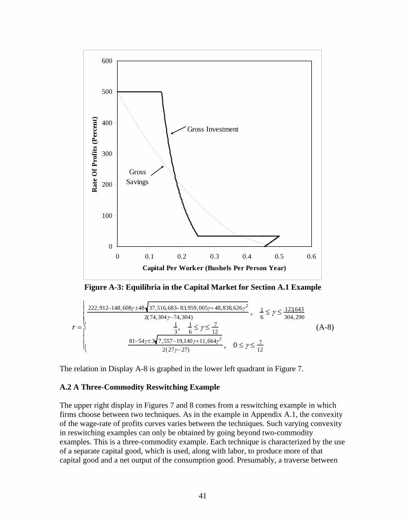
41

0

100

200

300

400

500

600

0 0.1 0.2 0.3 0.4 0.5 0.6

Capital Per Worker (Bushels Per Person Year)

Rat

e O

f Pro

fits (

Perc

ent)

Gross Investment

Gross Savings

Figure A-3: Equilibria in the Capital Market for Section A.1 Example

r =

222,912−148,608γ ±48 37,516,683−83,959,005γ +48,838,626γ 2

2(74,304γ −74,304), 1

6≤ γ ≤ 123,643

304,29013, 1

6≤ γ ≤ 7

1281−54γ ±3 7,557−19,140γ +11,664γ 2

2(27γ −27), 0 ≤ γ ≤ 7

12

⎧

⎨

⎪ ⎪ ⎪

⎩

⎪ ⎪ ⎪

(A-8)

The relation in Display A-8 is graphed in the lower left quadrant in Figure 7. A.2 A Three-Commodity Reswitching Example The upper right display in Figures 7 and 8 comes from a reswitching example in which firms choose between two techniques. As in the example in Appendix A.1, the convexity of the wage-rate of profits curves varies between the techniques. Such varying convexity in reswitching examples can only be obtained by going beyond two-commodity examples. This is a three-commodity example. Each technique is characterized by the use of a separate capital good, which is used, along with labor, to produce more of that capital good and a net output of the consumption good. Presumably, a traverse between

42

techniques would use an unmodeled backstop technology that allows one capital good to be produced with the aid of the other. The technology is specified by Displays A-9 through A-12. Displays A-9 and A-10 give the coefficients of production for the alpha technique:

a0

α = a01α a02

α a03α[ ]=

13

0 1⎡

⎣ ⎢ ⎢

⎤

⎦ ⎥ ⎥ (A-9)

Aα =

a11α a12

α a13α

a21α a22

α a23α

a31α a32

α a33α

⎡

⎣

⎢ ⎢ ⎢ ⎢

⎤

⎦

⎥ ⎥ ⎥ ⎥ =

16

0 1

0 0 00 0 0

⎡

⎣

⎢ ⎢ ⎢ ⎢ ⎢ ⎢

⎤

⎦

⎥ ⎥ ⎥ ⎥ ⎥ ⎥

(A-10)

Displays A-11 and A-12 give the coefficients of production for the alpha technique:

a0

β = a01β a02

β a03β[ ]= 0

12

32

⎡

⎣ ⎢ ⎢

⎤

⎦ ⎥ ⎥ (A-11)

Aβ =

a11β a12

β a13β

a21β a22

β a23β

a31β a32

β a33β

⎡

⎣

⎢ ⎢ ⎢ ⎢

⎤

⎦

⎥ ⎥ ⎥ ⎥ =

0 0 0

014

14

0 0 0

⎡

⎣

⎢ ⎢ ⎢ ⎢

⎤

⎦

⎥ ⎥ ⎥ ⎥ (A-12)

Tables A-3 and A-4 give the quantity flows per worker for stationary states in which the alpha and beta techniques, respectively, are adopted by cost minimizing firms. Display A-13 gives the wage-rate of profits frontier for this example:

w(r ) =

5− r7 + r

, 0 ≤ r ≤1 or 2 ≤ r ≤ 5

3 − r5 − r

, 1≤ r ≤ 2

⎧

⎨ ⎪ ⎪

⎩ ⎪ ⎪

(A-13)

The wage-rate of profits curves and the frontier are graphed in Figure A-4. The alpha technique minimizes costs for low and high rates of profits, while the beta technique minimizes costs at intermediate rates of profits. Display A-14 gives the price of the capital good used in the alpha technique:

p1(r ) =

27 + r

, 0 ≤ r ≤1 or 2 ≤ r ≤ 5 (A-14)

Display A-15 gives the price of the capital good used in the beta technique:

43

Table A-3: Quantity Flows for the Alpha Technique for Section A.2 Example Inputs Steel Industry Corn Industry Labor

27

Person-Year 57

Person-Year

Steel 17

Ton 57

Ton

Corn 0 Bushel 0 Bushel Outputs

67

Ton Steel 57

Bushels Corn

Capital per Worker: ( 67

Ton Seel, 0 Bushel)

Net Output Per Worker: 57

Bushel Corn

Table A-4: Quantity Flows for the Beta Technique for Section A.2 Example Inputs Tin Industry Corn Industry Labor

1

10 Person-Year

9

10 Person-Year

Tin 120

Ton 320

Ton

Corn 0 Bushel 0 Bushel Outputs

15

Ton Tin 35

Bushels Corn

Capital per Worker: ( 15

Ton Tin, 0 Bushel)

Net Output Per Worker: 35

Bushel Corn

44

0

0.1

0.2

0.3

0.4

0.5

0.6

0.7

0.8

0 100 200 300 400 500 600

Rate Of Profits (Percent)

Wag

e (B

ushe

ls C

orn

Per

Pers

on-Y

ear)

(100%, 1/2)

(200%, 1/3)

Alpha Technique is cost-minimizing

Alpha Technique is cost-minimizing

Beta Technique is cost-minimizing

Figure A-4: Wage-Rate of Profits Frontier for Section A.2 Example

p2 (r ) =

25 − r

, 1≤ r ≤ 2 (A-15)

The investment function for the example is specified in Display A-16:

I(r ) =

127(7 + r )

, 0 ≤ r ≤1 or 2 ≤ r ≤ 5

25(5 − r )

, 1 ≤ r ≤ 2

⎧

⎨ ⎪ ⎪

⎩ ⎪ ⎪

(A-16)

Figure A-5 graphs the investment function and two savings functions.39 The stationary state equilibrium rates of profits compatible with each value of the utility function are specified in Display A-17: 39 The lower savings function results from a value of γ of 24 / 35; the upper from a value of 18 / 35.

45

0

100

200

300

400

500

600

0 0.05 0.1 0.15 0.2 0.25 0.3 0.35 0.4

Capital Per Worker (Bushels Per Labor Year)

Rat

e O

f Pro

fits (

Perc

ent)

Gross Savings

Gross Investment

Figure A-5: Equilibria in the Capital Market for Section A.2 Example

r =

23−35γ7(1−γ )

, 0 ≤ γ ≤ 37

2, 37

≤ γ ≤ 35

13−15γ5(1−γ )

, 35

≤ γ ≤ 45

1, 47

≤ γ ≤ 45

23−35γ7(1−γ )

, 47

≤ γ ≤ 2335

⎧

⎨

⎪ ⎪ ⎪ ⎪ ⎪

⎩

⎪ ⎪ ⎪ ⎪ ⎪

(A-17)

The above relation is graphed in the upper right quadrant of Figure 7.

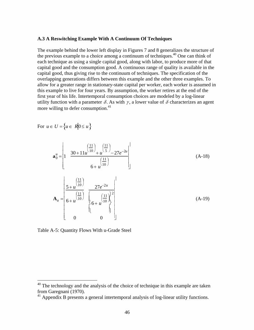
46

A.3 A Reswitching Example With A Continuum Of Techniques The example behind the lower left display in Figures 7 and 8 generalizes the structure of the previous example to a choice among a continuum of techniques.40 One can think of each technique as using a single capital good, along with labor, to produce more of that capital good and the consumption good. A continuous range of quality is available in the capital good, thus giving rise to the continuum of techniques. The specification of the overlapping generations differs between this example and the other three examples. To allow for a greater range in stationary-state capital per worker, each worker is assumed in this example to live for four years. By assumption, the worker retires at the end of the first year of his life. Intertemporal consumption choices are modeled by a log-linear utility function with a parameter δ . As with γ , a lower value of δ characterizes an agent more willing to defer consumption.41 For u ∈U = u ∈ R 0 ≤ u{ }

a0u = 1

30 +11u1110

⎛ ⎝ ⎜ ⎞

⎠ ⎟

+ u115

⎛ ⎝ ⎜ ⎞

⎠ ⎟

−27e−2u

6 + u1110

⎛ ⎝ ⎜ ⎞

⎠ ⎟

⎡

⎣

⎢ ⎢ ⎢ ⎢ ⎢

⎤

⎦

⎥ ⎥ ⎥ ⎥ ⎥

(A-18)

Au =

5 + u1110

⎛ ⎝ ⎜ ⎞

⎠ ⎟

6 + u1110

⎛ ⎝ ⎜ ⎞

⎠ ⎟

27e−2u

6 + u1110

⎛ ⎝ ⎜ ⎞

⎠ ⎟

⎧

⎨ ⎪ ⎪

⎩ ⎪ ⎪

⎫

⎬ ⎪ ⎪

⎭ ⎪ ⎪

2

0 0

⎡

⎣

⎢ ⎢ ⎢ ⎢ ⎢ ⎢ ⎢ ⎢ ⎢

⎤

⎦

⎥ ⎥ ⎥ ⎥ ⎥ ⎥ ⎥ ⎥ ⎥

(A-19)

Table A-5: Quantity Flows With u-Grade Steel

40 The technology and the analysis of the choice of technique in this example are taken from Garegnani (1970). 41 Appendix B presents a general intertemporal analysis of log-linear utility functions.

47

Table A-5: Quantity Flows With u-Grade Steel for Section A-3 Example

Inputs Steel Industry Corn Industry Labor

27e−2u

30 +11u1110

⎛ ⎝ ⎜ ⎞

⎠ ⎟

+ u115

⎛ ⎝ ⎜ ⎞

⎠ ⎟

Person-Year

30 +11u1110

⎛ ⎝ ⎜ ⎞

⎠ ⎟

+ u115

⎛ ⎝ ⎜ ⎞

⎠ ⎟

− 27e−2u

6 + u1110

⎛ ⎝ ⎜ ⎞

⎠ ⎟ ⎛

⎝

⎜ ⎜ ⎜ ⎜

⎞

⎠

⎟ ⎟ ⎟ ⎟

5+ u1110

⎛ ⎝ ⎜ ⎞

⎠ ⎟ ⎛

⎝

⎜ ⎜ ⎜ ⎜

⎞

⎠

⎟ ⎟ ⎟ ⎟

Person-Year

Steel

27e−2u

6 + u1110

⎛ ⎝ ⎜ ⎞

⎠ ⎟

⎛

⎝

⎜ ⎜ ⎜ ⎜

⎞

⎠

⎟ ⎟ ⎟ ⎟

2 Ton

27e−2u

6 + u1110

⎛ ⎝ ⎜ ⎞

⎠ ⎟

⎛

⎝

⎜ ⎜ ⎜ ⎜

⎞

⎠

⎟ ⎟ ⎟ ⎟

2

5+ u1110

⎛ ⎝ ⎜ ⎞

⎠ ⎟

⎛

⎝

⎜ ⎜ ⎜ ⎜

⎞

⎠

⎟ ⎟ ⎟ ⎟

Ton

Corn 0 Bushel 0 Bushel Outputs

27e−2u

30 +11u1110

⎛ ⎝ ⎜ ⎞

⎠ ⎟

+ u115

⎛ ⎝ ⎜ ⎞

⎠ ⎟

Ton Steel

1

5 + u1110

⎛ ⎝ ⎜ ⎞

⎠ ⎟ Bushels Corn

Capital per Worker: (

27e−2u

30 +11u1110

⎛ ⎝ ⎜ ⎞

⎠ ⎟

+ u115

⎛ ⎝ ⎜ ⎞

⎠ ⎟ Ton, 0 Bushel)

Net Output Per Worker: 1

5 + u1110

⎛ ⎝ ⎜ ⎞

⎠ ⎟ Bushel Corn

wu (r) =u

1110

⎛ ⎝ ⎜ ⎞

⎠ ⎟

r + 5r −1

u115

⎛ ⎝ ⎜ ⎞

⎠ ⎟

r +10u1110

⎛ ⎝ ⎜ ⎞

⎠ ⎟

r − u1110

⎛ ⎝ ⎜ ⎞

⎠ ⎟

+ 25r −5 −27re−2u

(A-20)

Figure A-6 graphs Equation A-20 for four values of u . The cost-minimizing outer envelope wage-rate of profits frontier is also shown. The wage-rate of profits curve for u = 0 is of a different convexity than the other three wage-rate of profits curve shown. The grade of steel in the cost-minimizing technique varies continuously along the frontier, with each cost-minimizing grade of steel used for a low and high rate of profits, except for u = u* ≈1.51. Since only one value of u is cost minimizing for each rate of profits, all points on the frontier are non-switching points. The cost-minimizing grade of steel is the value of u that results in equating the derivative of wu (r) with respect to u equal to zero. I solved this equation numerically, by Newton’s method.

48

0

0.04

0.08

0.12

0.16

0.2

0 5 10 15 20

Rate Of Profits (Percent)

Wag

e (B

ushe

ls P

er P

erso

n Y

ear)

Figure A-6: Wage-Rate of Profits Frontier for Section A.3 Example

Equation A-21 gives the stationary state price of steel:

pu (r) =−6 − u

1110

⎛ ⎝ ⎜ ⎞

⎠ ⎟

u115

⎛ ⎝ ⎜ ⎞

⎠ ⎟

r +10u1110

⎛ ⎝ ⎜ ⎞

⎠ ⎟

r − u1110

⎛ ⎝ ⎜ ⎞

⎠ ⎟

+ 25r −5 −27re−2u

(A-21)

Figure A-7 graphs the relationship between the labor-intensity of the stationary state cost-minimizing technique and the wage. Figure A-8 shows the investment function and three savings functions. All these curves are “smooth”.

49

0

0.05

0.1

0.15

0.2

0.25

0 1 2 3 4 5 6 7

Labor Intensity (Person-Years Per Bushel)

Wag

e (B

ushe

ls Pe

r Pe

rson

-Yea

r)

Figure A-7: Labor Intensity for Section A.3 Example

50

0

5

10

15

20

0 0.2 0.4 0.6 0.8 1 1.2

Capital Per Worker (Bushels Per Person Year)

Rat

e O

f Pro

fits

(Per

cent

)

Savings Function, δ = 0

Savings Function, δ = 1/4

Savings Function, δ = 11/20

Investment Function

Figure A-8: Equilibria in the Capital Market for Section A.3 Example

51

Appendix B: Stationary State Savings With Log-Linear Utility Function

Consider an agent, who lives n periods, deciding on an intertemporal consumption path. Assume the agent has a log-linear utility function. The agent, by assumption, works the first period and is retired the remaining periods. Given stationary prices, the agent must solve the mathematical programming problem in Display B-1: Choose c0 , c1, …, cn−1

To maximize U c0,c1,K,cn−1( )=

1(1+δ)i

ln ci( )i=0

n−1

∑ (B-1)

Such that

ci

(1+ r )ii=0

n−1

∑ = w

c0 ≥ 0 , c1 ≥ 0 , …, cn−1 ≥ 0 ; δ > 0 As δ becomes larger, the agent becomes more impatient. Display B-2 gives the marginal conditions:

∂U∂ci−1∂U∂ci

=(1+ δ)ci

ci−1=1+ r , i =1, 2,K , n −1 (B-2)

The marginal conditions allow one to express desired consumption in future years in terms of the consumption in the first year:

ci =

1+ r1+δ

⎛

⎝ ⎜ ⎜

⎞

⎠ ⎟ ⎟ i

c0 , i = 0, 1,K , n −1 (B-3)

Substituting consumption in future years into the budget constraint, one obtains B-4:

c0 =1

1(1+δ)i

i=0

n−1∑

w =δ(1+δ)n−1

(1+δ)n −1w (B-4)

Hence, consumption at the end of each year in the agent’s life is:

ci =

δ(1+δ)n−i−1

(1+δ)n −1(1+ r )i w, i = 0, 1,K , n −1 (B-5)

52

Table B-1 gives yearly consumption for the first few possibilities of the agent’s lifespan. Stationary state savings is found by adding up the savings of the different agents alive at the end of a given year:

S(r ) =

c j

(1+ r ) j−i +1j=i

n−1

∑i=1

n−1

∑ =w(r )

(1+δ)n −1(1+ δ)n−i −1[ ](1+ r )i−1

i=1

n−1

∑ (B-6)

Table B-2 gives savings functions for different agent lifespans.

Table B-1: Intertemporal Stationary State Consumption n c0 c1 c2 c3 1 w 2

1+ δ2 + δ

w 1+ r2 + δ

w

3

(1+δ)2

3 + 3δ +δ2w

(1+ δ)(1+ r )3 + 3δ + δ2

w

(1+ r )2

3 + 3δ +δ2w

4

(1+δ)3

4 + 6δ + 4δ2 +δ3w

(1+ δ)2(1+ r )4 + 6δ + 4δ2 +δ3

w

(1+ δ)(1+ r )2

4 + 6δ + 4δ2 +δ3w

(1+ r )3

4 + 6δ + 4δ2 +δ3w

Table B-2: Stationary State Savings Functions n Savings Function 1 S(r ) = 0 2

S(r ) =

12 + δ

w(r )

3

S(r ) =

3 +δ + r3 + 3δ + δ2

w(r )

4

S(r ) =

6 + 4δ + δ2 + 4r +δr + r 2

4 + 6δ + 4δ2 + δ3w(r )

5

S(r ) =

10 +10δ + 5δ2 +δ3 +10r + 5δr +δ2r + 5r 2 + r 2δ + r3

5+10δ +10δ2 + 5δ3 + δ4w(r )

53

Appendix C: Local Stability Analysis of Stationary States With One Technique

This appendix presents a local stability analysis of limit points to the dynamic process defined in Section 2. This analysis is confined to limit points corresponding to stationary states at non-switching points on the wage-rate of profits frontier. Such limit points are asymptotically stable if and only if both (?) of the following conditions are met:

1+ a11a12

<a01a02

(C-1)

(C-?) The condition in Display C-1 states that the ratio of surplus steel produced in the steel industry per ton output to the input of steel in the corn industry per bushel output falls below the ratio of labor inputs per unit output in the respective industries… These conclusions on stability follow from a common type of analysis for dynamic systems. The state variables of the original system are redefined in terms of deviations from the stationary state. The dynamic process is linearized around the stationary-state solution. Dynamic paths in this linearized system are stable if and only if the absolute values of the eigenvalues of the matrix characterizing the dynamics of this linear system are less than unity. C.1 Redefined State Variables Let c *, q*, p1 * , w*, r * be the stationary-state solution. Define some new variables in terms of the their deviations from the stationary-state solution: C(t ) = c(t ) − c * (C-2) Q(t ) = q(t ) − q* (C-3) P1(t ) = p1(t ) − p1 * (C-4) W( t ) = w(t ) − w * (C-5) R( t ) = r (t ) − r * (C-6)

This redefinition of variables leaves linear relations unchanged. Consider Equation 8. Equation C-7 follows from some algebraic manipulations:42

42 The index indicating the technique has been dropped from all equations in this appendix.

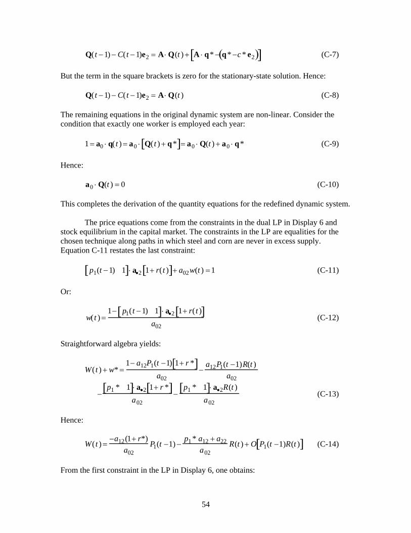
54

Q(t −1) − C(t −1)e2 = A ⋅ Q(t ) + A ⋅ q* − q* −c * e2( )[ ] (C-7) But the term in the square brackets is zero for the stationary-state solution. Hence: Q(t −1) − C( t −1)e2 = A ⋅ Q(t ) (C-8) The remaining equations in the original dynamic system are non-linear. Consider the condition that exactly one worker is employed each year: 1 = a0 ⋅ q( t ) = a0 ⋅ Q(t ) + q*[ ]= a0 ⋅ Q(t ) + a0 ⋅ q* (C-9) Hence: a0 ⋅ Q(t ) = 0 (C-10) This completes the derivation of the quantity equations for the redefined dynamic system. The price equations come from the constraints in the dual LP in Display 6 and stock equilibrium in the capital market. The constraints in the LP are equalities for the chosen technique along paths in which steel and corn are never in excess supply. Equation C-11 restates the last constraint: p1(t −1) 1[ ]⋅ a•2 1+ r(t )[ ]+ a02w(t ) =1 (C-11) Or:

w(t ) =

1− p1(t −1) 1[ ]⋅ a•2 1+ r(t )[ ]a02

(C-12)

Straightforward algebra yields:

W( t ) + w* =

1− a12P1(t −1) 1+ r *[ ]a02

−a12P1(t −1)R(t )

a02

−

p1 * 1[ ]⋅ a•2 1+ r *[ ]a02

−p1 * 1[ ]⋅ a•2R(t )

a02 (C-13)

Hence:

W( t ) =

−a12(1+ r*)a02

P1(t −1) −p1 * a12 + a22

a02R(t ) + O P1(t −1)R(t )[ ] (C-14)

From the first constraint in the LP in Display 6, one obtains:

55

p1(t −1) 1[ ]⋅ a•1 1+ r (t )[ ]+ a01w(t ) = p1(t ) (C-15) Substituting for the wage, one obtains:

p1(t ) =

a01 − p1(t −1) 1[ ]⋅ a01a•2 − a02a•1( ) 1+ r(t )[ ]a02

(C-16)

Some algebra yields:

P1(t ) + p1* =

−P1(t −1) a12a01 − a11a02( ) 1+ r *[ ]a02

−

P1( t −1) a12a01 − a11a02( )R( t )a02

+a01 − p1 * 1[ ]⋅ a01a•2 − a02a•1( ) 1+ r *[ ]

a02

−

p1 * 1[ ]⋅ a01a•2 − a02a•1( )R(t )a02

(C-17)

Or:

P1(t ) =

− a01a12 − a02a11( ) 1+ r *[ ]a02

P1(t −1)

−

p1 * 1[ ]⋅ a01a•2 − a02a•1( )a02

R( t ) + O P1( t −1)R(t )[ ] (C-18)

Equation 13 implies Equation C-19 gives gross savings: (1− γ)w(t ) = (1− γ)W( t ) + (1− γ)w* , (C-19) Substituting for the wage, one obtains:

S( t ) =

−a12(1− γ)P1(t −1) 1+ r *[ ]− p1 * 1[ ]⋅ a•2 (1− γ)R( t )a02

+O P1(t −1)R(t )[ ]+ (1−γ)w* (C-20) Equation C-21 restates Equation 7, which gives the value of gross investment, in terms of deviations from the stationary state: I(t ) = P1(t ) 0[ ]+ p1 * 1[ ]{ }⋅ Q(t ) − C( t )e2 + q* −c * e2[ ] (C-21) The usual algebra yields, for the investment function, the following equation: I(t ) = P1(t )q1 * + p1 * Q1(t ) + Q2 (t ) − C( t ) + P1(t )Q1(t )

56

+ p1 * 1[ ]⋅ q* −c * e2[ ] (C-22) Linearizing the stock equilibrium condition that households are willing to hold the value of the capital goods, one obtains Equation C-23:

−a12(1−γ ) 1+ r *[ ]a02

P1(t −1) −p1 * a12 + a22[ ](1− γ)

a02R(t )

≈ q1 * P1(t ) + p1 * Q1( t) + Q2(t ) −C(t ) (C-23) C.2 The Linearized System The dynamical system determines six state variables at moment in time: Q1(t ) , Q2 (t ) ,

C(t ), P1(t ) , W(t ), and R(t ). Dropping second order terms, one finds six equations determine the system: two equations in Display C-8 and the equations in Displays C-10, C-14, C-18, and C-23. The values of the state variables during the previous year determine their values at the current year. Thus, given initial values for these variables and the above linear system of six equations, the equilibrium time path of these variables is uniquely determined. This dynamical system can be further simplified into two equations determining the dynamic paths of a quantity and of a price variable. All other state variables can be found as a function of the two chosen variables. The quantity equations (C-8 and C-10) can be solved first. I have chosen to express all variables in terms of the deviation of the time path of the output of the consumption good, corn, from the stationary-state solution. Equation C-30 specifies the time path of the gross outputs of corn around the stationary state:

Q2 (t ) =

−a02a01a12 − a02a11

Q2(t −1) (C-24)

Equations C-25 and C-26 determine the deviations of the time path of the output of steel and of the consumption of corn, respectively, from the stationary-state solution:

Q1(t ) =

−a02a01

Q2(t ) (C-25)

C(t ) = 1+

a02a01

(a01a22 − a02a21)(a01a12 − a02a11)

⎡

⎣ ⎢ ⎢

⎤

⎦ ⎥ ⎥ Q2(t ) (C-26)

These equations are easy to understand. By assumption, firms produce both corn and steel along equilibrium time paths in this model. Labor is fully employed, and firms anticipate the future so well that neither produced steel nor corn is in excess supply at any point in time. Along such paths, if more steel than the stationary-state quantity is produced, less corn than the stationary-state quantity is produced, so as to ensure full

57

employment. This full employment condition determines the ratio, at any time, of steel production to corn production. The additional condition that steel and corn capital be fully used determines the time path of corn production and consumption. The linearized price equations are not nearly as intuitive. Equation C-27 characterizes the dynamic path of the deviation of the price of steel from the stationary-state solution, in terms of the deviation of the output of corn, the stationary-state rate of profits, and the coefficients of production:

P1(t ) ≈ a02

2 a01a12 + a02(1− a11)[ ]{

× a01(a01a12 − a02a11) + a02(a01a22 − a02a21)[ ]2

× (a11a22 − a12a21)(1+ r*)2 − (a11 + a22)(1+ r*) +1[ ]}

a01(a01a12 − a02a11)2 (a01a12 − a02a11)(1+ r*) + a02[ ]( 2

× (a11a22 − a12a21) a02(a11a22 − a12a21)[{

−(a01a12 + a02a22)](1+ r*)

+(a01a12 + a02a22) a12a21 + a22(1− a11)[ ]

+a12(a01a11 + a02a21)})Q2(t −1)

+ (1+ r*)(a11a22 − a12a21)(

× (a01a12 + a02a22 ) − a02(a11a22 − a12a21){

−(a11a22 − a12a21) a01a12 + a02(1− a11)[ ](1+ r*)})

(a11a22 − a12a21) a02(a11a22 − a12a21)[{

−(a01a12 + a02a22)](1+ r*)

+(a01a12 + a02a22) a12a21 + a22(1− a11)[ ]

+a12(a01a11 + a02a21)}P1(t −1) (C-27) Equation C-28 gives the deviation of the rate of profits from the stationary-state value:

R(t ) ≈ −

a02p1 * a01a12 − a02a11( )+ a01a22 − a02a21( )P1(t )

−

a01a12 − a02a11( ) 1+ r *[ ]p1 * a01a12 − a02a11( )+ a01a22 − a02a21( )P1(t −1) (C-28)

Equation C-28 could be further simplified to express the current deviation of the rate of profits in terms of the current deviations of the output of corn and the price of steel, the stationary-state rate of profits, and the coefficients of production alone. One would achieve this simplification by substituting into Equation C-28 the stationary-state price of steel and the lagged deviation of the price of steel. Equation C-14 gives the deviation of

58

the wage from the stationary-state solution as a function of the deviations of the price of the steel and the rate of profits. This equation could also be simplified such that the deviation of the wage depends only on current values of the deviations of the output of corn and the price of steel and the same set of system parameters as in Display C-28. C.3 Local Stability Analysis Section C.2 has shown that the local stability analysis of a stationary state reduces to the consideration of the stability of the deviation from the stationary-state solution of the time paths of the output of corn and the price of steel. The matrix expressing the system dynamics of the linearized system is decomposable, thus allowing the stability of each of these two state variables to be analyzed separately. The quantity variables in a stationary state are stable if and only if the inequality in Display C-29 holds:

−a02a01a12 − a02a11

<1 (C-29)

Given stable quantity variables, the price variables in a stationary state are stable if and only if the inequality in Display C-30 holds:

(1+ r*)(a11a22 − a12a21)(

× (a01a12 + a02a22 ) − a02(a11a22 − a12a21){

−(a11a22 − a12a21) a01a12 + a02(1− a11)[ ](1+ r*)})

(a11a22 − a12a21) a02(a11a22 − a12a21) − (a01a12 + a02a22 )[ ]{ (1+ r*)

+(a01a12 + a02a22) a12a21 + a22(1− a11)[ ]

+a12(a01a11 + a02a21)}<1 (C-30)

C.3.1 Stability of Quantity Variables Two cases arise for the analysis of the quantity system. For the first case, suppose the quantity whose absolute value is taken in Display C-29 is positive. In other words, the denominator is negative: a01a12 − a02a11 < 0 (C-31) Or:

a12a02

<a11a01

(C-32)

In this case, the inequality in Display C-29 is equivalent to:

59

a12a02

< −1− a11

a01 (C-33)

But the left hand side is non-negative and the right hand side, for a viable economy, is negative. So this case is impossible. For the second case, suppose the absolute value in C-29 is taken for a negative quantity:

a11a01

<a12a02

(C-34)

The inequality becomes:

1+ a11a01

<a12a02

(C-35)

Note that since labor inputs are positive, the inequality in Display C-35 implies the inequality in Display C-34. So the inequality in Display C-35 is a sufficient and necessary condition that the quantity variables on dynamic equilibrium paths near a stationary state converge to the stationary-state values. C.3.2 Stability of Price Variables Two cases arise, also, for the stability of price variables. References Albin, P. S. (1975). “Reswitching: An Empirical Observation, A Theoretical Note, and an

Environmental Conjecture”, Kyklos, V. 28: 149-153. Bharadwaj, K. (1989). Themes in Value and Distribution: Classical Theory Reappraised,

London: Unwin Hyman. Blaug, M. (1975). The Cambridge Revolution: Success or Failure? A Critical Analysis of

Cambridge Theories of Value and Distribution (Revised Edition). The Institute of Economic Affairs.

Bliss, C. J. (1975). Capital Theory and the Distribution of Income, Amsterdam: North

Holland Press. Bloise, G. and Richlin, P. (2005). “An Obtrusive Remark on Capital and Comparative

Statics” (Preliminary draft), 26 Apr.

60

Burmeister, E. (1980). Capital Theory and Dynamics. Cambridge: Cambridge University Press.

Cohen, A. J. and Harcourt, G. C. (2003). “Whatever Happened to the Cambridge Capital

Theory Controversies?” Journal of Economic Perspectives, V. 17, N. 1 (Winter): 199-214.

Debreu, G. (1959). Theory of Value: An Axiomatic Analysis of Economic Equilibrium,

New Haven: Yale University Press. Dixit, A. (1977). “The Accumulation of Capital Theory”, Oxford Economic Papers, New

Series, V. 29, N. 1 (Mar.): 1-29. Ferretti, M. (2004). “The Neo-Ricardian Critique: An Anniversary Assessment”,

University of Rome seminar, 26 Oct. Friedman, D. D. (1990). Price Theory: An Intermediate Text, Second Edition, Cincinnati:

South-Western Publishing. Garegnani, P. (1970). “Heterogeneous Capital, the Production Function and the Theory

of Distribution”, Review of Economic Studies, V. 37, N. 3 (Jul): 407-436. Garegnani, P. (1976). “On a Change in the Notion of Equilibrium in Recent Work on

Value and Distribution”, reprinted in Keynes’s Economics and the Theory of Value and Distribution (edited by J. L. Eatwell and M. Milgate, 1983), Oxford University Press.

Garegnani, P. (1984). “Value and Distribution in Classical Economics and Marx,” Oxford

Economic Papers. V. 36, pp. 291-325. Garegnani, P. (1990a). “Sraffa: Classical versus Marginal Analysis,” in Essays on Piero

Sraffa: Critical Perspectives on the Revival of Classical Theory, (edited by K. Bharadway and B. Schefold). Unwin Hyman.

Garegnani, P. (1990b). “Quantity of Capital”, in The New Palgrave: Capital Theory

(Edited by J. Eatwell, M. Milgate, and P. Newman), New York: W. W. Norton. Gram, H. (1995). “The Role of Perfect Foresight in Krishna Bharadwaj’s Critique of

Demand and Supply Equilibrium-Based Theory”, in The Classical Tradition in Economic Thought (edited by I. H. Rima), Brookfield, VT: Edward Elgar.

Grandmont, J. M. (1977). “Temporary General Equilibrium Theory”, Econometrica, V.

45, N. 3 (Apr): 535-572. Guckenheimer, J. and Holmes, P. (1983). Nonlinear Oscillations, Dynamical Systems,

and Bifurcations of Vector Fields, New York: Springer-Verlag.

61

Hahn, F. (1982). “The Neo-Ricardians”, Cambridge Journal of Economics, V. 6: 353-

374. Han, Z. and Schefold, B. (2003). “An Empirical Investigation of Paradoxes (Reswitching

and Reverse Capital Deepening) in Capital Theory”, Sep. Harcourt, G. C. (1969). “Some Cambridge Controversies in the Theory of Capital”,

Journal of Economic Literature, June. Hayek, F. A. (1945). “The Use of Knowledge in Society”, American Economic Review,

V. 35, N. 4 (Sept.): 519-530. Hicks, J. R. (1946). Value and Capital: An Inquiry into Some Fundamental Principles of

Economic Theory, Second Edition, Oxford: Oxford University Press. Kahn, R. F. (1959). “Exercises in the Analysis of Growth”, Oxford Economic Papers,

New Series V. 11, N. 2 (Jun.): 143-156. Kaldor, N. (1955-56). “Alternative Theories of Distribution”, Review of Economic

Studies, V. 23, N. 2 (Jun.): 83-100. Kaldor, N. (1966). “Marginal Productivity and the Macro-economic Theories of

Distribution”, Review of Economic Studies, V. 33, N. 4 (Oct.): 309-319. Kirman, A. P. (1992). “Whom or What does the Representative Individual Represent?”

Journal of Economic Perspectives, V. 6: 117-136. Kurz, H. D. and Salvadori, N. (1995). Theory of Production: A Long-Period Analysis.

Cambridge University Press. Marglin, S. A. (1984). Growth, Distribution, and Prices, Cambridge: Harvard University

Press. Marshall, A. (1920). Principles of Economics: An Introductory Volume, Eighth edition.

Macmillan. Mas-Colell, A. (1989). “Capital Theory Paradoxes: Anything Goes”, in Joan Robinson

and Modern Economic Theory (ed. by G. Feiwel), New York: New York University Press.

Milgate, M. (1979). “On the Origin of the Notion of ‘Intertemporal Equilibrium’”,

Economica, V. 46, N. 1: 1-10.

62

Ozanne, A. (1996). “Do Supply Curves Slope Up? The Empirical Relevance of the Sraffian Critique of Neoclassical Production Economics”, Cambridge Journal of Economics, V. 20: 749-762.

Panico, C. (1999). “The Government Sector in the Post-Keynesian Theory of Growth and

Personal Distribution”, in Value, Distribution, and Capital: Essays in Honour of Pierangelo Garegnani, (edited by G. Mongiovi and F. Petri), New York: Routledge.

Pasinetti, L. L. (1962). “Rate of Profit and Income Distribution in Relation to the Rate of

Economic Growth”, Review of Economic Studies, V. 29, N. 4 (Oct.): 267-279. Pasinetti, L. L. (1977). “On ‘Non-Substitution’ in Production Models,” Cambridge

Journal of Economics. V. 1, pp. 389-394. Pasinetti, L. L. (editor) (1980). Essays on the Theory of Joint Production. Columbia

University Press. Pasinetti, L. L. (2005). “The Cambridge School of Keynesian Economics”, Cambridge

Journal of Economics, V. 29: 837-848. Petri, F. (2004). General Equilibrium, Capital and Macroeconomics: A Key to Recent

Controversies in Equilibrium Theory, Northampton, MA: Edward Elgar. Prince, R. and Rosser, J. B., Jr. (1985). “Some Implications of Delayed Environmental

Costs for Benefit Cost Analysis: A Study of Reswitching in the Western Coal Lands”, Growth and Change, V. 16: 18-25.

Robinson, J. (1962). Essays in the Theory of Economic Growth, London: Macmillan. Robinson, J. V. (1974). “History Versus Equilibrium”, Indian Economic Journal, V. 21

(Mar.): 202-213. Samuelson, P. A. (1966). “A Summing Up”, Quarterly Journal of Economics, V. 80, N. 4

(Nov.): 568-583. Samuelson, P. A. (1975). “Steady-State and Transient Relations: A Reply on

Reswitching”, Quarterly Journal of Economics, V. 89, N. 1 (Feb.): 40-47. Samuelson, P. A. (2001). “A Modern Post-Mortem on Bohm’s Capital Theory: Its Vital

Normative Flaw Shared by Pre-Sraffian Mainstream Capital Theory”, Journal of the History of Economic Thought, V. 23, N. 3: 301-307.

Smith, A. (1937). An Inquiry into the Nature and Causes of the Wealth of Nations,

Modern Library edition, New York: Random House.

63

Solow, R. M. (1975). “Brief Comments”, Quarterly Journal of Economics, V. 89, N. 1 (Feb.): 48-52.

Sraffa, P. (1960). Production of Commodities by Means of Commodities: A Prelude to a

Critique of Economic Theory, Cambridge: Cambridge University Press. Schefold, B. (1989). Mr. Sraffa on Joint Production and Other Essays. Unwin Hyman. Schefold, B. (2000). “Paradoxes of Capital and Counterintuitive Changes of Distribution

in an Intertemporal Equilibrium Model”, in Critical Essays on Piero Sraffa’s Legacy in Economics, (edited by H. D. Kurz), Cambridge: Cambridge University Press.

Sharpe, K. (1999). “On Sraffa’s Price System”, Cambridge Journal of Economic, V. 23:

93-101. Steedman, I. (editor) (1988). Sraffian Economics, (Two volumes). Edward Elgar. Steedman, I. (1998). “Classical Economics and Marginalism”, in The Elgar Companion

to Classical Economics (Edited by H. D. Kurz and N. Salvadori), Northampton, Massachusetts: Edward Elgar.

Stiglitz, J. E. (1974). “The Cambridge-Cambridge Controversy in the Theory of Capital:

A View from New Haven: A Review Article”, The Journal of Political Economy, V. 82: 893-903.

Velupillai, K. V. (2005). “The Unreasonable Ineffectiveness of Mathematics in

Economics”, Cambridge Journal of Economics, V. 29: 849-872. Vienneau, R. L. (2005a). “On Labour Demand and Equilibria of the Firm”. The

Manchester School, V. 73, N. 5 (Sep.): 612-619. Vienneau, R. L. (2005b). “Creating Two-Good Reswitching Examples”, (Aug),

<http://papers.ssrn.com/sol3/papers.cfm?abstract_id=687492> Zambelli, S. (2004). “The 40% Neoclassical Aggregate Theory of Production”,

Cambridge Journal of Economics, V. 28, N. 1 (Jan.): 99-120.