manifold regularization: a geometric framework for...

Manifold Regularization: A Geometric Frameworkfor Learning from Examples

Mikhail Belkin�, Partha Niyogi�, Vikas Sindhwani�

The University of ChicagoHyde Park, Chicago, IL 60637

�misha,niyogi,vikass�@cs.uchicago.edu

August 25, 2004

Abstract

We propose a family of learning algorithms based on a new form of regu-larization that allows us to exploit the geometry of the marginal distribution.We focus on a semi-supervised framework that incorporates labeled and un-labeled data in a general-purpose learner. Some transductive graph learningalgorithms and standard methods including Support Vector Machines andRegularized Least Squares can be obtained as special cases. We utilize prop-erties of Reproducing Kernel Hilbert spaces to prove new Representer theo-rems that provide theoretical basis for the algorithms. As a result (in contrastto purely graph based approaches) we obtain a natural out-of-sample exten-sion to novel examples and so are able to handle both transductive and trulysemi-supervised settings. We present experimental evidence suggesting thatour semi-supervised algorithms are able to use unlabeled data effectively. Fi-nally we have a brief discussion of unsupervised and fully supervised learn-ing within our general framework.

1 Introduction

In this paper, we introduce a new framework for data-dependent regularization thatexploits the geometry of the probability distribution. While this framework allowsus to approach the full range of learning problems from unsupervised to supervised,we focus on the problem of semi-supervised learning. The problem of learning

�Department of Computer Science, also TTI Chicago�Departments of Computer Science and Statistics�Department of Computer Science, also TTI Chicago

1

from labeled and unlabeled data (semi-supervised and transductive learning) hasattracted considerable attention in recent years. Some recently proposed methodsinclude Transductive SVM [35, 22], Cotraining [13], and a variety of graph basedmethods [12, 14, 32, 37, 38, 24, 23, 4]. We also note two regularization basedtechniques [16, 7]. The latter reference is closest in spirit to the intuitions of ourpaper.

The idea of regularization has a rich mathematical history going back to [34],where it is used for solving ill-posed inverse problems. Regularization is a key ideain the theory of splines (e.g., [36]) and is widely used in machine learning (e.g.,[20]). Many machine learning algorithms, including Support Vector Machines, canbe interpreted as instances of regularization.

Our framework exploits the geometry of the probability distribution that gener-ates the data and incorporates it as an additional regularization term. Hence, thereare two regularization terms — one controlling the complexity of the classifier inthe ambient space and the other controlling the complexity as measured by the ge-ometry of the distribution. We consider in some detail the special case where thisprobability distribution is supported on a submanifold of the ambient space.

The points below highlight several aspects of the current paper:

1. Our general framework brings together three distinct concepts that have re-ceived some independent recent attention in machine learning:i. The first of these is the technology of spectral graph theory (e.g., see [15])that has been applied to a wide range of clustering and classification tasksover the last two decades. Such methods typically reduce to certain eigen-value problems.ii. The second is the geometric point of view embodied in a class of algo-rithms that can be termed as manifold learning (see webpage [39] for a fairlylong list of references). These methods attempt to use the geometry of theprobability distribution by assuming that its support has the geometric struc-ture of a Riemannian manifold.iii. The third important conceptual framework is the set of ideas surroundingregularization in Reproducing Kernel Hilbert Spaces. This leads to the classof kernel based algorithms for classification and regression (e.g., see [31],[36], [20]).

We show how to bring these ideas together in a coherent and natural way toincorporate geometric structure in a kernel based regularization framework.As far as we know, these ideas have not been unified in a similar fashionbefore.

2. Within this general framework, we propose two specific families of algo-

2

rithms: the Laplacian Regularized Least Squares (hereafter LapRLS) andthe Laplacian Support Vector Machines (hereafter LapSVM). These are nat-ural extensions of RLS and SVM respectively. In addition, several recentlyproposed transductive methods (e.g., [38, 4]) are also seen to be special casesof this general approach.

3. We elaborate on the RKHS foundations of our algorithms and show howgeometric knowledge of the probability distribution may be incorporated insuch a setting. In particular, a new Representer theorem provides a functionalform of the solution when the distribution is known and an empirical versionwhich involves an expansion over labeled and unlabeled points when thedistribution is unknown. These Representer theorems provide the basis forour algorithms.

4. Our framework with an ambiently defined RKHS and the associated Repre-senter theorems result in a natural out-of-sample extension from the data set(labeled and unlabeled) to novel examples. This is in contrast to the varietyof purely graph based approaches that have been considered in the last fewyears. Such graph based approaches work in a transductive setting and donot naturally extend to the semi-supervised case where novel test examplesneed to be classified (predicted). Also see [8, 11] for some recent relatedwork on out-of-sample extensions.

1.1 The Significance of Semi-Supervised Learning

From an engineering standpoint, it is clear that collecting labeled data is generallymore involved than collecting unlabeled data. As a result, an approach to patternrecognition that is able to make better use of unlabeled data to improve recognitionperformance is of potentially great practical significance.

However, the significance of semi-supervised learning extends beyond purelyutilitarian considerations. Arguably, most natural (human or animal) learning oc-curs in the semi-supervised regime. We live in a world where we are constantlyexposed to a stream of natural stimuli. These stimuli comprise the unlabeled datathat we have easy access to. For example, in phonological acquisition contexts, achild is exposed to many acoustic utterances. These utterances do not come withidentifiable phonological markers. Corrective feedback is the main source of di-rectly labeled examples. In many cases, a small amount of feedback is sufficient toallow the child to master the acoustic-to-phonetic mapping of any language.

The ability of humans to do unsupervised learning (e.g. learning clusters andcategories of objects) suggests that unlabeled data can be usefully processed tolearn natural invariances, to form categories, and to develop classifiers. In most

3

pattern recognition tasks, humans have access only to a small number of labeledexamples. Therefore the success of human learning in this “small sample” regimeis plausibly due to effective utilization of the large amounts of unlabeled data toextract information that is useful for generalization.

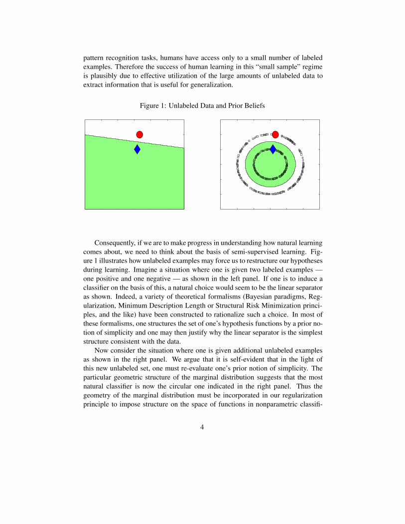
Figure 1: Unlabeled Data and Prior Beliefs

Consequently, if we are to make progress in understanding how natural learningcomes about, we need to think about the basis of semi-supervised learning. Fig-ure 1 illustrates how unlabeled examples may force us to restructure our hypothesesduring learning. Imagine a situation where one is given two labeled examples —one positive and one negative — as shown in the left panel. If one is to induce aclassifier on the basis of this, a natural choice would seem to be the linear separatoras shown. Indeed, a variety of theoretical formalisms (Bayesian paradigms, Reg-ularization, Minimum Description Length or Structural Risk Minimization princi-ples, and the like) have been constructed to rationalize such a choice. In most ofthese formalisms, one structures the set of one’s hypothesis functions by a prior no-tion of simplicity and one may then justify why the linear separator is the simpleststructure consistent with the data.

Now consider the situation where one is given additional unlabeled examplesas shown in the right panel. We argue that it is self-evident that in the light ofthis new unlabeled set, one must re-evaluate one’s prior notion of simplicity. Theparticular geometric structure of the marginal distribution suggests that the mostnatural classifier is now the circular one indicated in the right panel. Thus thegeometry of the marginal distribution must be incorporated in our regularizationprinciple to impose structure on the space of functions in nonparametric classifi-

4

cation or regression. This is the intuition we formalize in the rest of the paper.The success of our approach depends on whether we can extract structure fromthe marginal distribution and on the extent to which such structure may reveal theunderlying truth.

1.2 Outline of the Paper

The paper is structured as follows: in Sec. 2, we develop the basic frameworkfor semi-supervised learning where we ultimately formulate an objective functionthat can utilize both labeled and unlabeled data. The framework is developed inan RKHS setting and we state two kinds of Representer theorems describing thefunctional form of the solutions. In Sec. 3, we elaborate on the theoretical under-pinnings of this framework and prove the Representer theorems of Sec. 2. Whilethe Representer theorem for the finite sample case can be proved using standardorthogonality arguments, the Representer theorem for the known marginal distri-bution requires more subtle considerations. In Sec. 4, we derive the different algo-rithms for semi-supervised learning that arise out of our framework. Connectionsto related algorithms are stated. In Sec. 5, we describe experiments that evaluatethe algorithms against each other and demonstrate the usefulness of unlabeled data.In Sec. 6, we consider the cases of fully supervised and unsupervised learning. InSec. 7 we conclude.

2 The Semi-Supervised Learning Framework

2.1 Background

Recall the standard framework of learning from examples. There is a probabilitydistribution � on � � � according to which examples are generated for functionlearning. Labeled examples are �� pairs generated according to � . Unlabeledexamples are simply � � � drawn according to the marginal distribution �� of� .

One might hope that knowledge of the marginal �� can be exploited for betterfunction learning (e.g. in classification or regression tasks). Of course, if there isno identifiable relation between �� and the conditional ��, the knowledge of�� is unlikely to be of much use.

Therefore, we will make a specific assumption about the connection betweenthe marginal and the conditional distributions. We will assume that if two points�� are close in the intrinsic geometry of �� , then the conditional distribu-tions �� and �� are similar. In other words, the conditional probability

5

distribution �� varies smoothly along the geodesics in the intrinsic geometryof �� .

We utilize these geometric intuitions to extend an established framework forfunction learning. A number of popular algorithms such as SVM, Ridge regres-sion, splines, Radial Basis Functions may be broadly interpreted as regularizationalgorithms with different empirical cost functions and complexity measures in anappropriately chosen Reproducing Kernel Hilbert Space (RKHS).

For a Mercer kernel � � � � � � �, there is an associated RKHS �� offunctions � � � with the corresponding norm � �� . Given a set of labeled exam-ples �� , � � �� the standard framework estimates an unknown functionby minimizing

� � ��

�

�

��

�� (1)

where is some loss function, such as squared loss �� for RLS or the

soft margin loss function for SVM. Penalizing the RKHS norm imposes smooth-ness conditions on possible solutions. The classical Representer Theorem statesthat the solution to this minimization problem exists in �� and can be written as

��

��

�� (2)

Therefore, the problem is reduced to optimizing over the finite dimensional spaceof coefficients ��, which is the algorithmic basis for SVM, Regularized LeastSquares and other regression and classification schemes.

We first consider the case when the marginal distribution is already known.

2.2 Marginal �� is known

Our goal is to extend this framework by incorporating additional information aboutthe geometric structure of the marginal �� . We would like to ensure that the solu-tion is smooth with respect to both the ambient space and the marginal distribution�� . To achieve that, we introduce an additional regularizer:

� � ��

�

�

��

�� (3)

where �� is an appropriate penalty term that should reflect the intrinsic structureof �� . Here �� controls the complexity of the function in the ambient space while�� controls the complexity of the function in the intrinsic geometry of �� . It turns

6

out that one can derive an explicit functional form for the solution � as shown inthe following theorem.

Theorem 2.1. Assume that the penalty term �� is sufficiently smooth with re-spect to the RKHS norm �� . Then the solution � to the optimization problemin Eqn. 3 above exists and admits the following representation

��

��

��

�� (4)

where � � � �� is the support of the marginal �� .

We postpone the proof and the exact formulation of smoothness conditions onthe norm � �� until the next section.

The Representer Theorem above allows us to express the solution � directlyin terms of the labeled data, the (ambient) kernel � , and the marginal �� . If ��is unknown, we see that the solution may be expressed in terms of an empiricalestimate of �� . Depending on the nature of this estimate, different approximationsto the solution may be developed. In the next section, we consider a particularapproximation scheme that leads to a simple algorithmic framework for learningfrom labeled and unlabeled data.

2.3 Marginal �� Unknown

In most applications the marginal �� is not known. Therefore we must attempt toget empirical estimates of �� and � �� . Note that in order to get such empiricalestimates it is sufficient to have unlabeled examples.

A case of particular recent interest (e.g., see [27, 33, 5, 19] for a discussionon dimensionality reduction) is when the support of �� is a compact submanifold��

� . In that case, one natural choice for �� is�� .

The optimization problem becomes

� � ��

�

�

��

��

��

The term�� may be approximated on the basis of labeled and

unlabeled data using the graph Laplacian ([4], also see [7]). Thus, given a set of �labeled examples �� and a set of � unlabeled examples �� , weconsider the following optimization problem :

� � ��

�

�

��

��

��

��

��

7

� ��

�

�

��

��

�� (5)

where �� are edge weights in the data adjacency graph, � � �� ,

and � is the graph Laplacian given by � � �� . Here, the diagonal matrix D isgiven by ��

�� . The normalizing coefficient �

�� is the natural scalefactor for the empirical estimate of the Laplace operator. We note than on a sparseadjacency graph it may be replaced by

�� .

The following version of the Representer Theorem shows that the minimizerhas an expansion in terms of both labeled and unlabeled examples and is a key toour algorithms.

Theorem 2.2. The minimizer of optimization problem 5 admits an expansion

��

��

�� (6)

in terms of the labeled and unlabeled examples.

The proof is a variation of the standard orthogonality argument and is presentedin Section 3.4.Remark 1: Several natural choices of � �� exist. Some examples are:

1. Iterated Laplacians ��. Differential operators �� and their linear combina-tions provide a natural family of smoothness penalties.

2. Heat semigroup �� is a family of smoothing operators corresponding tothe process of diffusion (Brownian motion) on the manifold. One can take��

�� . We note that for small values of � the corresponding

Green’s function (the heat kernel of �) can be approximated by a sharpGaussian in the ambient space.

3. Squared norm of the Hessian (cf. [19]). While the Hessian �� (the matrixof second derivatives of ) generally depends on the coordinate system, itcan be shown that the Frobenius norm (the sum of squared eigenvalues) of� is the same in any geodesic coordinate system and hence is invariantlydefined for a Riemannian manifold �. Using the Frobenius norm of � asa regularizer presents an intriguing generalization of thin-plate splines. Wealso note that �� .

Remark 2: Note that � restricted to� (denoted by ��) is also a kernel definedon� with an associated RKHS�� of functions �� . While this might sug-gest �� (� is restricted to�) as a reasonable choice for �� ,

8

it turns out, that for the minimizer � of the corresponding optimization problemwe get �� , yielding the same solution as standard regularization, al-though with a different �. This observation follows from the restriction propertiesof RKHS discussed in the next section and is formally stated as Proposition 3.4.Therefore it is impossible to have an out-of-sample extension without two differentmeasures of smoothness. On the other hand, a different ambient kernel restricted to� can potentially serve as the intrinsic regularization term. For example, a sharpGaussian kernel can be used as an approximation to the heat kernel on�.

3 Theoretical Underpinnings and Results

In this section we briefly review the theory of Reproducing Kernel Hilbert spacesand their connection to integral operators. We proceed to establish the Representertheorems from the previous section.

3.1 General Theory of RKHS

We start by recalling some basic properties of Reproducing Kernel Hilbert Spaces(see the original work [2] and also [17] for a nice discussion in the context of learn-ing theory) and their connections to integral operators. We say that a Hilbert space� of functions � � � has the reproducing property, if �� the evaluationfunctional � �� is continuous. For the purposes of this discussion we willassume that � is compact. By Riesz Representation theorem it follows that for agiven � � � , there is a function �� , s.t.

� � � ��

We can therefore define the corresponding kernel function

�� It follows that �� and thus �� . It isclear that �� .

It can be easily shown that �� is a positive semi-definite kernel, i.e., thatgiven � points �� , the corresponding matrix � with �� ispositive semi-definite. Moreover, if the space � is sufficiently rich, that is if forany �� there is a function , s.t. �� , then �

is strictly positive definite. Conversely any function �� with such propertygives rise to an RKHS. For simplicity we will assume that all our RKHS are rich(the corresponding kernels are sometimes called universal).

9

We proceed to endow � with a measure � (supported on all of �). We denotethe corresponding Hilbert norm by �� .

We can now consider the integral operator �� corresponding the kernel �:

��

��

It is well-known that this operator is compact and self-adjoint with respect to ��and, by the Spectral Theorem, its eigenfunctions �� form an orthog-onal basis of �� and the corresponding eigenvalues �� are discrete withfinite multiplicity, �� .

We see that��

and therefore �� . Writing a function in that basis, we

have ��

�� and �� . Assuming that �� ,

which can be ensured by extending �, if necessary, we see that

��

��

Therefore �� , if � �� , and ��

. On the other hand�� , if � �� , and �� . This observation establishes a sim-ple relationship between the Hilbert norms in � and ��. We also see that ��

�� if and only if� ��

��.

Consider now the operator �� . It can be defined as the only positive definite

self-adjoint operator, s.t. �� Æ ��

� . Assuming that the series ��

�� converges, we can write

��

��

It is easy to check that �� is an isomorphism between � and ��, that is

��

��

Therefore � is the image �� acting on ��.

Lemma 3.1. A function �� can be represented as � �� for

some � if and only if��

��

�� (7)

10

Proof. Suppose � ��. Write �� . We know that � � ��

� ifand only if

��

�� . Since ��

��

��

�� , we obtain

�� . Therefore��

��

��.

Conversely, if the condition in the inequality 7 is satisfied, � ��, where� �

� ��.

3.2 Proof of Theorems

Now let us recall the Eqn. 3:

� � ��

�

�

��

�� (8)

We have an RKHS �� and the probability distribution � which is supported on� � � . We define a linear space � to be the closure with respect to the RKHSnorm of�� of the linear span of kernels centered at points of �:

� � ��

Before we start we need to introduce some notation. By a subscript � we willdenote the restriction to �. For example, by �� we denote the restriction offunctions from � to �. It can be shown ([2], p. 350) that the space ��of functions from �� restricted to � is an RKHS with the kernel ��, in otherwords �� .

Lemma 3.2. The following properties of � hold:

1. � with the inner product induced by �� is a Hilbert space.

2. �� .

3. The orthogonal complement � to � in�� consists of all functions vanish-ing on �.

Proof. 1. From the definition of � it is clear by that � is a complete subspace of�� .

2. We give a convergence argument similar to one found in [2]. Since �� any function � in it can be written as � � �� , where �� is the sum of some kernel functions.Consider the corresponding sum � �

�� . From the definition

of the norm we see that �� and therefore � is aCauchy sequence. Thus � �� exists and its restriction to�must equal

11

�. This shows that �� . The other direction follows by the sameargument.

3. Let � � �. By the reproducing property for any � � �, �� and therefore any function in � vanishes on �. On theother hand, if � vanishes on � it is perpendicular to each �� and istherefore perpendicular to the closure of their span � .

Lemma 3.3. Assume that the intrinsic norm is such that for any � � � �� , � �� implies that �� . Then if the solution �, of the optimizationproblem in Eqn. 8 exists and belongs to � .

Proof. Any � �� can be written as � � � � , where � is the projection of to � and � is its orthogonal complement.

For any � �� we have �� . By the previous Lemma � vanishes on�. We have �� and by assumption �� .

On the other hand, �� and therefore �� .It follows that the minimizer � is in � .

As a direct corollary of these consideration, we obtain the following

Proposition 3.4. If �� then the minimizer of Eqn. 8 is identical tothat of the usual regularization problem (Eqn. 1) although with a different regular-ization parameter.

We can now restrict our attention to the study of � . While it is clear that theright-hand side of Eqn. 4 lies in � , not every element in � can be written like that.For example, �� , where � is not one of the data points �� is generally not ofthat form.

We will now assume that for � �

�� where � is an appropriate smoothness operator, such as an inverse integral oper-ator or a differential operator, e.g., � � �� . The Representer theorem,however, holds for even more general �:

Theorem 3.5. Let � be a bounded operator � � � � �� . Then the solution �

of the optimization problem in Eqn. 3 exists and can be written

��

��

��

�� (9)

12

Proof. For simplicity we will assume that the loss function is differentiable.This condition can ultimately be eliminated by approximating a non-differentiablefunction appropriately and passing to the limit.

Put

��

�

��

�� (10)

We first show that the solution to Eqn. 3 � exists and by Lemma 3.3 belongsto � . It follow easily from Cor. 3.7 and standard results about compact embeddingsof Sobolev spaces (e.g., [1]) that a ball �� , �� !is compact in �� . Therefore for any such ball the minimizer in that ball �� mustexist and belong to ��. On the other hand, by substituting the zero function

��

�

��

��

If the loss is actually zero, then zero function is a solution, otherwise

��

��

��

and hence �� , where

! �

��

��

Therefore we cannot decrease �� by increasing ! beyond a certain point, whichshows that � � �� with ! as above, which completes the proof of existence. If is convex, such solution will also be unique.

We proceed to derive the Eqn. 9. As before, let �� be the basis as-sociated to the integral operator ��

�� . Write

� �� . By substituting � into �� we obtain:

��

�

��

��

��

Assume that is differentiable with respect to each ��. We have ��

. Differentiating with respect to the coefficients �� yields the following setof equations:

"��

"��

�

�

��

��"� ��

��

��

13

where "� denotes the derivative with respect to the third argument of .�� and hence

��

��

��

��"� ��

��

Since �� and recalling that ��

��

��

��

��

��

��"� ��

��

��

��

� � �

��

��

�� "� ��

��

��

��

We see that the first summand is a sum of the kernel functions centered at datapoints. It remains to show that the second summand has an integral representation,i.e. can be written as

�� , which is equivalent to being in the

image of �� . To verify this we apply Lemma 3.1. We need that

��

��

��

�� (11)

Since �, its adjoint operator �� and hence their sum are bounded the inequality 11is satisfied for any function in � .

3.3 Manifold Setting1

We now show that for the case when � is a manifold and � is a differentialoperator, such as the Laplace-Beltrami operator �, the boundedness condition ofTheorem 3.5 is satisfied. While we consider the case when the manifold has noboundary, the same argument goes through for manifold with boundary, with, forexample, Dirichet’s boundary conditions (vanishing at the boundary). Thus thesetting of Theorem 3.5 is very general, applying, among other things, to arbitrarydifferential operators on compact domains in Euclidean space.

Let� be a � manifold without boundary with an infinitely differentiable em-bedding in some ambient space � , � a differential operator with � coefficientsand let �, be the measure corresponding to some � nowhere vanishing volume

1We thank Peter Constantin and Todd Dupont for help with this section.

14

form on �. We assume that the kernel �� is also infinitely differentiable.2

As before for an operator #, #� denotes the adjoint operator.

Proof. First note that it is enough to show that � is bounded on �� , since �

only depends on the restriction �. As before, let��

is the integral operator associated to �� . Note that �� is also a differential opera-tor of the same degree as �. The integral operator �� is bounded (compact) from�� to any Sobolev space ��. Therefore the operator �� is also bounded. We

therefore see that �� is bounded ��

�. Therefore there is a constant$ , s.t. �� $�� .

The square root % � ��

of the self-adjoint positive definite operator �� isa self-adjoint positive definite operator as well. Thus ��% �� %��. By definitionof the operator norm, for any & � � there exists � �� &, such that

��%�� %�� %�� %��

� �� $�� &��

Therefore the operator �% � �� is bounded (and also ��%�� $ ,

since & is arbitrary).Now recall that % provides an isometry between �� and �� . That means

that for any � � �� there is � ��, such that % � � and ��

.

Thus �� %�� $��, which shows that % � ��

� isbounded and concludes the proof.

Since � is a subspace of �� the main result follows immediately:

Corollary 3.6. � is a bounded operator � � �� and the conditions of Theo-rem 3.5 hold.

Before finishing the theoretical discussion we obtain a useful

Corollary 3.7. The operator % � �� on ��

� is a bounded (and in fact compact)operator ��

� � ��, where �� is an arbitrary Sobolev space.

Proof. Follows from the fact that �% is bounded operator �� for an ar-

bitrary differential operator � and standard results on compact embeddings ofSobolev spaces (see, e.g. [1]).

2While we have assumed that all objects are infinitely differentiable, it is not hard to specify theprecise differentiability conditions. Roughly speaking, a degree � differential operator � is boundedas an operator ��

�, if the kernel �� has �� derivatives.

15

3.4 The Representer Theorem for the Empirical Case

In the case when� is unknown and sampled via labeled and unlabeled examples,the Laplace-Beltrami operator on � may be approximated by the Laplacian ofthe data adjacency graph (see [3, 7] for some discussion). A regularizer basedon the graph Laplacian leads to the optimization problem posed in Eqn. 5. Wenow provide a proof of Theorem 2.2 which states that the solution to this problemadmits a representation in terms of an expansion over labeled and unlabeled points.The proof is based on a simple orthogonality argument (e.g., [31]).

Proof. (Theorem 2.2) Any function � �� can be uniquely decomposed into acomponent in the linear subspace spanned by the kernel functions �� ,and a component orthogonal to it. Thus,

� � ��

��

By the reproducing property, as the following arguments show, the evaluationof on any data point �� , � � � � � � � is independent of the orthogonal compo-nent :

��

��

Since the second term vanishes, and �� , it followsthat ��

�� . Thus, the empirical terms involving the loss

function and the intrinsic norm in the optimization problem in Eqn. 5 depend onlyon the value of the coefficients �� and the gram matrix of the kernel function.

Indeed, since the orthogonal component only increases the norm of in �� :��

�� , it follows that

the minimizer of problem 5 must have � �, and therefore admits a representa-tion ��

�� .The simple form of the minimizer, given by this theorem, allows us to translate

our extrinsic and intrinsic regularization framework into optimization problemsover the finite dimensional space of coefficients �� , and invoke the machineryof kernel based algorithms. In the next section, we derive these algorithms, andexplore their connections to other related work.

16

4 Algorithms

We now discuss standard regularization algorithms (RLS and SVM) and presenttheir extensions (LapRLS and LapSVM respectively). These are obtained by solv-ing the optimization problems posed in Eqn. (5) for different choices of cost func-tion and regularization parameters �� . To fix notation, we assume we have� labeled examples �� and � unlabeled examples �� . We use �

interchangeably to denote the kernel function or the Gram matrix.

4.1 Regularized Least Squares

The Regularized Least Squares algorithm is a fully supervised method where wesolve :

��

�

�

��

�� (12)

The classical Representer Theorem can be used to show that the solution is ofthe following form:

��

��

�� (13)

Substituting this form in the problem above, we arrive at following convexdifferentiable objective function of the �-dimensional variable � � ��

� :

��

��' �� ' �� (14)

where K is the � � � gram matrix �� and Y is the label vector' � ��

� .The derivative of the objective function vanishes at the minimizer :

�

��' ��

which leads to the following solution.

�� (��' (15)

4.2 Laplacian Regularized Least Squares (LapRLS)

The Laplacian Regularized Least Squares algorithm solves problem (5) with thesquared loss function:

17

��

�

�

��

��

��

��

As before, the Representer Theorem can be used to show that the solution is anexpansion of kernel functions over both the labeled and the unlabeled data :

��

��

�� (16)

Substituting this form in the problem above, as before, we arrive at a convexdifferentiable objective function of the ��-dimensional variable � � ��

� :

��

�

��' � )�� ' � )��

��

��

where K is the �� Gram matrix over labeled and unlabeled points; Yis an �� dimensional label vector given by : ' � �� and )

is an �� diagonal matrix given by ) � �� withthe first � diagonal entries as 1 and the rest 0.

The derivative of the objective function vanishes at the minimizer :

�

��' � )�� )��

��

��

which leads to the following solution.

�� )� � ��( ��

�� ' (17)

Note that when �� , Eqn. (17) gives zero coefficients over unlabeled data,and the coefficients over the labeled data are exactly those for standard RLS.

4.3 Support Vector Machine Classification

Here we outline the SVM approach to binary classification problems. For SVMs,the following problem is solved :

��

�

�

��

��

where the hinge loss is defined as: �� *�� and thelabels �� .

18

Again, the solution is given by:

��

��

�� (18)

Following SVM expositions, the above problem can be equivalently written as:

��

�

�

��

+� � �� (19)

subject to : �� +� � � ��

+� � � � � ��

Using the Lagrange multipliers technique, and benefiting from strong duality,the above problem has a simpler quadratic dual program in the Lagrange multipli-ers , � �,�� ,��

� � �� :

,� � ��

��

,� � �

�,�-, (20)

subject to :��

��,� � �

� � ,� � �

��

where the equality constraint arises due to an unregularized bias term that is oftenadded to the sum in Eqn (18), and the following notation is used :

' � ��

- � '

��

��

�'

�� ' ,�

��(21)

Here again, K is the gram matrix over labeled points. SVM practitioners maybe familiar with a slightly different parameterization involving the $ parameter :$ � �

�� is the weight on the hinge loss term (instead of using a weight � on thenorm term in the optimization problem). The $ parameter appears as the upperbound (instead of �

� ) on the values of , in the quadratic program. For additionaldetails on the derivation and alternative formulations of SVMs, see [31], [26].

19

4.4 Laplacian Support Vector Machines

By including the intrinsic smoothness penalty term, we can extend SVMs by solv-ing the following problem:

��

�

�

��

��

��

By the representer theorem,as before, the solution to the problem above is givenby:

��

��

��

Often in SVM formulations, an unregularized bias term � is added to the aboveform. Again, the primal problem can be easily seen to be the following:

��

�

�

��

+� � ��

��

��

subject to : ��

�� +��

+� � � � � ��

Introducing the Lagrangian, with ,�� .� as Lagrange multipliers:

�� +� �� ,� .� ��

�

��

+� ��

��

��

��

��

,��

�� +��

.�+�

Passing to the dual requires the following steps:

"�

"��

��

,��

"�

"+��

�� ,� � .� � �

�� ,� � �

�(+�� .� are non-negative)

20

Using above identities, we formulate a reduced Lagrangian:

� �� ,� ��

��

��

��

��

,��

��

��

��

��

��

�� )�' , �

��

,� (22)

where ) � �( �� is an �� matrix with ( as the �� identity matrix (assumingthe first l points are labeled) and ' � �� .

Taking derivative of the reduced Lagrangian wrt �:

"�

"��

��

�� )�' ,

This implies:

� � ��( � ��

�� )�' ,� (23)

Note that the relationship between � and , is no longer as simple as the SVMalgorithm. In particular, the �� expansion coefficients are obtained by solvinga linear system involving the � dual variables that will appear in the SVM dualproblem.

Substituting back in the reduced Lagrangian we get:

,� � ��

��

,� � �

�,�-, (24)

subject to :��

,��

� � ,� � �

�� (25)

where

- � ' )��( � ��

�� )�'

Laplacian SVMs can be implemented by using a standard SVM solver with thequadratic form induced by the above matrix, and using the solution to obtain theexpansion coefficients by solving the linear system in Eqn (23).

21

Note that when �� , the SVM QP and Eqns (24,23), give zero expansioncoefficients over the unlabeled data. The expansion coefficients over the labeleddata and the Q matrix are as in standard SVM, in this case.

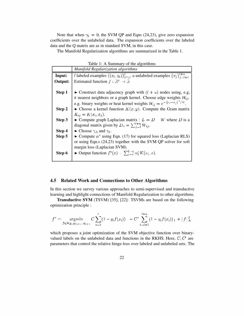
The Manifold Regularization algorithms are summarized in the Table 1.

Table 1: A Summary of the algorithmsManifold Regularization algorithms

Input: � labeled examples �� , � unlabeled examples ��Output: Estimated function � ��

Step 1 � Construct data adjacency graph with �� nodes using, e.g,/ nearest neighbors or a graph kernel. Choose edge weights �� ,e.g. binary weights or heat kernel weights ��

�� .Step 2 � Choose a kernel function �� . Compute the Gram matrix

�� .Step 3 � Compute graph Laplacian matrix : � � � �� where � is a

diagonal matrix given by �� .

Step 4 � Choose �� and �� .Step 5 � Compute �� using Eqn. (17) for squared loss (Laplacian RLS)

or using Eqn.s (24,23) together with the SVM QP solver for softmargin loss (Laplacian SVM).

Step 6 � Output function ��

�� .

4.5 Related Work and Connections to Other Algorithms

In this section we survey various approaches to semi-supervised and transductivelearning and highlight connections of Manifold Regularization to other algorithms.

Transductive SVM (TSVM) [35], [22]: TSVMs are based on the followingoptimization principle :

� � �� !!!��

$

��

�� $��

��

which proposes a joint optimization of the SVM objective function over binary-valued labels on the unlabeled data and functions in the RKHS. Here, $�$� areparameters that control the relative hinge-loss over labeled and unlabeled sets. The

22

joint optimization is implemented in [22] by first using an inductive SVM to labelthe unlabeled data and then iteratively solving SVM quadratic programs, at eachstep switching labels to improve the objective function. However this procedure issusceptible to local minima and requires an unknown, possibly very large numberof label switches before converging. Note that even though TSVM were inspiredby transductive inference, they do provide an out-of-sample extension.

Semi-Supervised SVMs (S�VM) [10], [21] : S�VM incorporate unlabeleddata by including the minimum hinge-loss for the two choices of labels for eachunlabeled example. This is formulated as a mixed-integer program for linear SVMsin [10] and is found to be intractable for large amounts of unlabeled data. [21]reformulate this approach as a concave minimization problem which is solved bya successive linear approximation algorithm. The presentation of these algorithmsis restricted to the linear case.

Measure-Based Regularization [7]: The conceptual framework of this workis closest to our approach. The authors consider a gradient based regularizer thatpenalizes variations of the function more in high density regions and less in lowdensity regions leading to the following optimization principle:

� � ��

��

��

�� 0��

where 0 is the density of the marginal distribution �� . The authors observe thatit is not straightforward to find a kernel for arbitrary densities 0, whose associ-ated RKHS norm is

� � �� 0�� . Thus, in the absence of a repre-senter theorem, the authors propose to perform minimization of the regularizedloss on a fixed set of basis functions chosen apriori, i.e, � � �"

�� 1�. Forthe hinge loss, this paper derives an SVM quadratic program in the coefficients��"�� whose - matrix is calculated by computing 2� integrals over gradientsof the basis functions. However the algorithm does not demonstrate performanceimprovements in real world experiments. It is also worth noting that while [7] usethe gradient �� in the ambient space, we use the gradient over a submanifold�� for penalizing the function. In a situation where the data truly lies on ornear a submanifold �, the difference between these two penalizers can be signif-icant since smoothness in the normal direction to the data manifold is irrelevant toclassification or regression.

Graph Based Approaches See e.g., [12, 14, 32, 37, 38, 24, 23, 4]: A varietyof graph based methods have been proposed for transductive inference. However,these methods do not provide an out-of-sample extension. In [38], nearest neighborlabeling for test examples is proposed once unlabeled examples have been labeledby transductive learning. In [14], test points are approximately represented as a

23

linear combination of training and unlabeled points in the feature space induced bythe kernel. Manifold regularization provides natural out-of-sample extensions toseveral graph based approaches. These connections are summarized in Table 2. Wealso note the very recent work [8] on out-of-sample extensions for semi-supervisedlearning. For Graph Regularization and Label Propagation see [29, 6, 38].

Cotraining [13] The Co-training algorithm was developed to integrate abun-dance of unlabeled data with availability of multiple sources of information in do-mains like web-page classification. Weak learners are trained on labeled examplesand their predictions on subsets of unlabeled examples are used to mutually expandthe training set. Note that this setting may not be applicable in several cases ofpractical interest where one does not have access to multiple information sources.

Bayesian Techniques See e.g., [25, 28, 16]. An early application of semi-supervised learning to Text classification appeared in [25] where a combinationof EM algorithm and Naive-Bayes classification is proposed to incorporate unla-beled data. [28] provides a detailed overview of Bayesian frameworks for semi-supervised learning. The recent work in [16] formulates a new information-theoretic principle to develop a regularizer for conditional log-likelihood.

Table 2: Connections of Manifold Regularization to other algorithmsParameters Corresponding algorithms (square loss or hinge loss)

�� Manifold Regularization�� Standard Regularization (RLS or SVM)�� Out-of-sample extension for Graph Regularization

(RLS or SVM)�� Out-of-sample extension for Label Propagation�� (RLS or SVM)�� Hard margin SVM or Interpolated RLS

5 Experiments

We performed experiments on a synthetic dataset and three real world classifica-tion problems arising in visual and speech recognition, and text categorization.Comparisons are made with inductive methods (SVM, RLS). Based on a surveyof related approaches, as summarized in Section 4.5, we chose to also compareLaplacian SVM with Transductive SVM. Other approaches lack out-of-sample ex-tension, use different base-classifiers or paradigms, or are implementationally notpreferable. All software and datasets used for these experiments will be made

24

available at:http://manifold.cs.uchicago.edu/manifold regularization/manifold.html.

5.1 Synthetic Data : Two Moons Dataset

The two moons dataset is shown in Figure 2. The dataset contains �� exampleswith only � labeled example for each class. Also shown are the decision surfacesof Laplacian SVM for increasing values of the intrinsic regularization parameter�� . When �� , Laplacian SVM disregards unlabeled data and returns the SVMdecision boundary which is fixed by the location of the two labeled points. As�� is increased, the intrinsic regularizer incorporates unlabeled data and causesthe decision surface to appropriately adjust according to the geometry of the twoclasses.

In Figure 3, the best decision surfaces across a wide range of parameter set-tings are also shown for SVM, Transductive SVM and Laplacian SVM. Figure 3demonstrates how TSVM fails to find the optimal solution. The Laplacian SVMdecision boundary seems to be intuitively most satisfying.

Figure 2: Laplacian SVM with RBF Kernels for various values of �� . Labeledpoints are shown in color, other points are unlabeled.

−1 0 1 2

−1

0

1

2

γA = 0.03125 γ

I = 0

SVM

−1 0 1 2

−1

0

1

2

Laplacian SVM

γA = 0.03125 γ

I = 0.01

−1 0 1 2

−1

0

1

2

Laplacian SVM

γA = 0.03125 γ

I = 1

5.2 Handwritten Digit Recognition

In this set of experiments we applied Laplacian SVM and Laplacian RLSC al-gorithms to �� binary classification problems that arise in pairwise classificationof handwritten digits. The first �� images for each digit in the USPS trainingset (preprocessed using PCA to �� dimensions) were taken to form the training

25

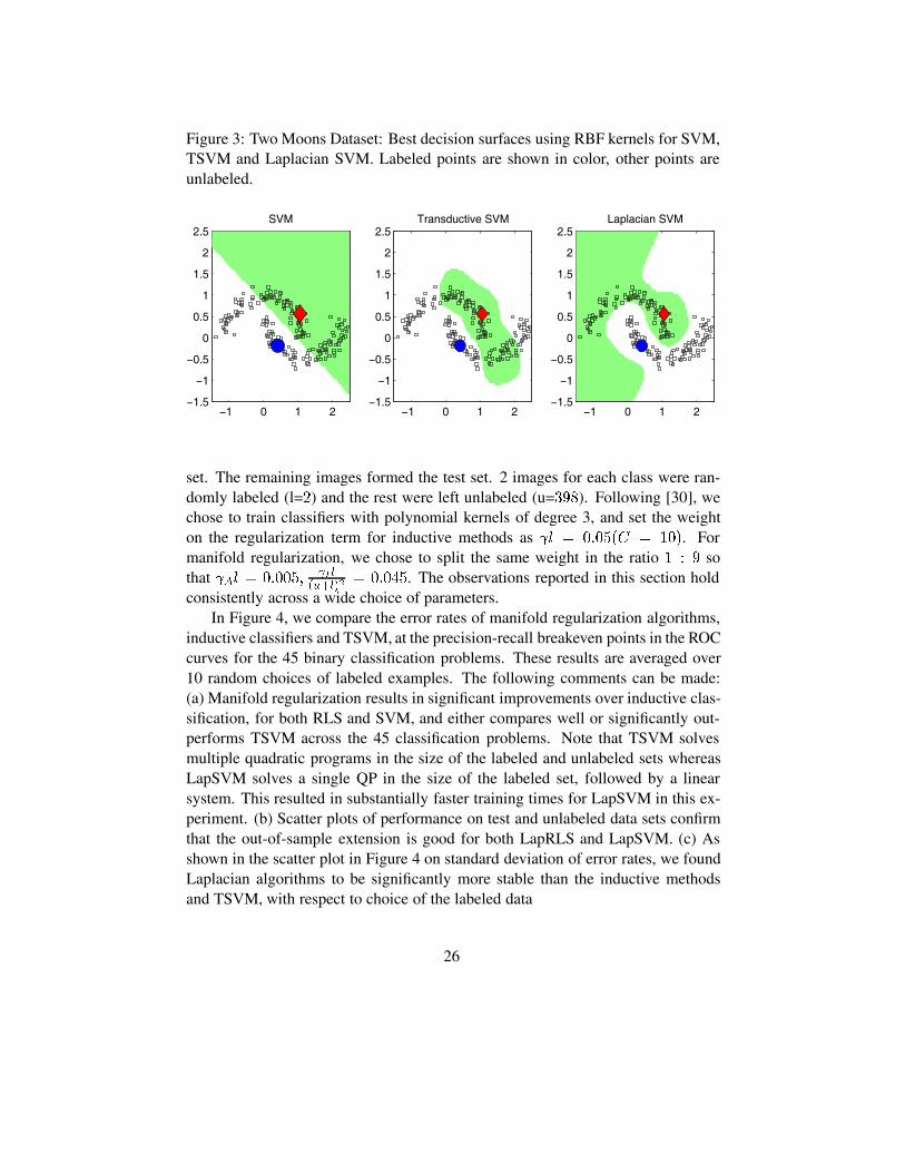
Figure 3: Two Moons Dataset: Best decision surfaces using RBF kernels for SVM,TSVM and Laplacian SVM. Labeled points are shown in color, other points areunlabeled.

−1 0 1 2−1.5

−1

−0.5

0

0.5

1

1.5

2

2.5SVM

−1 0 1 2−1.5

−1

−0.5

0

0.5

1

1.5

2

2.5Transductive SVM

−1 0 1 2−1.5

−1

−0.5

0

0.5

1

1.5

2

2.5Laplacian SVM

set. The remaining images formed the test set. 2 images for each class were ran-domly labeled (l=�) and the rest were left unlabeled (u=��). Following [30], wechose to train classifiers with polynomial kernels of degree 3, and set the weighton the regularization term for inductive methods as �� $ � ��. Formanifold regularization, we chose to split the same weight in the ratio � � � sothat ��

�� . The observations reported in this section hold

consistently across a wide choice of parameters.In Figure 4, we compare the error rates of manifold regularization algorithms,

inductive classifiers and TSVM, at the precision-recall breakeven points in the ROCcurves for the 45 binary classification problems. These results are averaged over10 random choices of labeled examples. The following comments can be made:(a) Manifold regularization results in significant improvements over inductive clas-sification, for both RLS and SVM, and either compares well or significantly out-performs TSVM across the 45 classification problems. Note that TSVM solvesmultiple quadratic programs in the size of the labeled and unlabeled sets whereasLapSVM solves a single QP in the size of the labeled set, followed by a linearsystem. This resulted in substantially faster training times for LapSVM in this ex-periment. (b) Scatter plots of performance on test and unlabeled data sets confirmthat the out-of-sample extension is good for both LapRLS and LapSVM. (c) Asshown in the scatter plot in Figure 4 on standard deviation of error rates, we foundLaplacian algorithms to be significantly more stable than the inductive methodsand TSVM, with respect to choice of the labeled data

26

Figure 4: USPS Experiment - Error Rates at Precision-Recall Breakeven points for45 binary classification problems

10 20 30 400

5

10

15

20

RLS vs LapRLS

45 Classification Problems

Erro

r Rat

es

RLSLapRLS

10 20 30 400

5

10

15

20

SVM vs LapSVM


Erro

r Rat

es

SVMLapSVM

10 20 30 400

5

10

15

20TSVM vs LapSVM


Erro

r Rat

es

TSVMLapSVM

0 5 10 150

5

10

15Out−of−Sample Extension

LapRLS (Unlabeled)

LapR

LS (T

est)

0 5 10 150

5

10

15Out−of−Sample Extension

LapSVM (Unlabeled)

LapS

VM (T

est)

0 2 4 60

5

10

15Std Deviation of Error Rates

SVM

(o) ,

TSV

M (x

) Std

Dev

LapSVM Std Dev

In Figure 5, we demonstrate the benefit of unlabeled data as a function of thenumber of labeled examples.

5.3 Spoken Letter Recognition

This experiment was performed on the Isolet database of letters of the Englishalphabet spoken in isolation (available from the UCI machine learning repository).The data set contains utterances of �� subjects who spoke the name of each letterof the English alphabet twice. The speakers are grouped into � sets of �� speakerseach, referred to as isolet1 through isolet5. For the purposes of this experiment,we chose to train on the first �� speakers (isolet1) forming a training set of ��examples, and test on isolet5 containing �� examples (1 utterance is missingin the database due to poor recording). We considered the task of classifying thefirst �� letters of the English alphabet from the last ��. The experimental set-upis meant to simulate a real-world situation: we considered �� binary classificationproblems corresponding to �� splits of the training data where all �� utterancesof one speaker were labeled and all the rest were left unlabeled. The test set iscomposed of entirely new speakers, forming the separate group isolet5.

27

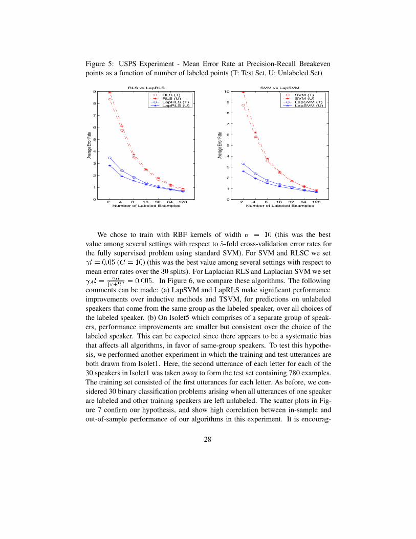
Figure 5: USPS Experiment - Mean Error Rate at Precision-Recall Breakevenpoints as a function of number of labeled points (T: Test Set, U: Unlabeled Set)

2 4 8 16 32 64 1280

1

2

3

4

5

6

7

8

9

10SVM vs LapSVM

Number of Labeled Examples

Avera

ge Er

ror R

ate

SVM (T)SVM (U)LapSVM (T)LapSVM (U)

2 4 8 16 32 64 1280

1

2

3

4

5

6

7

8

9RLS vs LapRLS


Avera

ge Er

ror R

ateRLS (T)RLS (U)LapRLS (T)LapRLS (U)

We chose to train with RBF kernels of width 3 � �� (this was the bestvalue among several settings with respect to �-fold cross-validation error rates forthe fully supervised problem using standard SVM). For SVM and RLSC we set�� ($ � ��) (this was the best value among several settings with respect tomean error rates over the �� splits). For Laplacian RLS and Laplacian SVM we set��

��

� ��. In Figure 6, we compare these algorithms. The followingcomments can be made: (a) LapSVM and LapRLS make significant performanceimprovements over inductive methods and TSVM, for predictions on unlabeledspeakers that come from the same group as the labeled speaker, over all choices ofthe labeled speaker. (b) On Isolet5 which comprises of a separate group of speak-ers, performance improvements are smaller but consistent over the choice of thelabeled speaker. This can be expected since there appears to be a systematic biasthat affects all algorithms, in favor of same-group speakers. To test this hypothe-sis, we performed another experiment in which the training and test utterances areboth drawn from Isolet1. Here, the second utterance of each letter for each of the30 speakers in Isolet1 was taken away to form the test set containing 780 examples.The training set consisted of the first utterances for each letter. As before, we con-sidered 30 binary classification problems arising when all utterances of one speakerare labeled and other training speakers are left unlabeled. The scatter plots in Fig-ure 7 confirm our hypothesis, and show high correlation between in-sample andout-of-sample performance of our algorithms in this experiment. It is encourag-

28

0 10 20 30

14

16

18

20

22

24

26

28

Labeled Speaker #

Erro

r Rat

e (u

nlab

eled

set

)

RLS vs LapRLS

RLSLapRLS

0 10 20 30

15

20

25

30

35

40

Labeled Speaker #

Erro

r Rat

es (u

nlab

eled

set

)

SVM vs TSVM vs LapSVM

SVMTSVMLapSVM

0 10 20 30

20

25

30

35

Labeled Speaker #

Erro

r Rat

es (t

est s

et)

RLS vs LapRLS

RLSLapRLS

0 10 20 30

20

25

30

35

40

Labeled Speaker #Er

ror R

ates

(tes

t set

)

SVM vs TSVM vs LapSVM

SVMTSVMLapSVM

Figure 6: Isolet Experiment - Error Rates at precision-recall breakeven points of30 binary classification problems

ing to note performance improvements with unlabeled data in Experiment 1 wherethe test data comes from a slightly different distribution. This robustness is oftendesirable in real-world applications.

5.4 Text Categorization

We performed Text Categorization experiments on the WebKB dataset which con-sists of 1051 web pages collected from Computer Science department web-sitesof various universities. The task is to classify these webpages into two categories:course or non-course. We considered learning classifiers using only textual contentof the webpages, ignoring link information. A bag-of-word vector space represen-tation for documents is built using the the top 3000 words (skipping HTML head-ers) having highest mutual information with the class variable, followed by TFIDFmapping. Feature vectors are normalized to unit length. 9 documents were foundto contain none of these words and were removed from the dataset.

For the first experiment, we ran LapRLS and LapSVM in a transductive set-

29

15 20 25 3015

20

25

30

Error Rate (Unlabeled)

Erro

r Rat

e (T

est)

RLS

Experiment 1Experiment 2

15 20 25 3015

20

25

30


Erro

r Rat

e (T

est)

LapRLS


15 20 25 3015

20

25

30


Erro

r Rat

e (T

est)

SVM


15 20 25 3015

20

25

30

Error Rate (Unlabeled)Er

ror R

ate

(Tes

t)

LapSVM


Figure 7: Isolet Experiment - Error Rates at precision-recall breakeven points onTest set Versus Unlabeled Set. In Experiment 1, the training data comes from Isolet1 and the test data comes from Isolet5; in Experiment 2, both training and test setscome from Isolet1.

ting, with 12 randomly labeled examples (3 course and 9 non-course) and the restunlabeled. In Table 1, we report the precision and error rates at the precision-recallbreakeven point averaged over 100 realizations of the data, and include results re-ported in [23] for Spectral Graph Transduction, and the Cotraining algorithm [12]for comparison. We used 15 nearest neighbor graphs, weighted by cosine distancesand used iterated graph Laplacians of degree 3. For inductive methods, �� wasset to �� for RLS and �� for SVM. For LapRLS and LapSVM, �� was set asin inductive methods, with ��

�� . These parameters were chosen based

on a simple grid search for best performance over the first 5 realizations of the data.Linear Kernels and cosine distances were used since these have found wide-spreadapplications in text classification problems [18].

Since the exact datasets on which these algorithms were run, somewhat dif-fer in preprocessing, preparation and experimental protocol, these results are onlymeant to suggest that Manifold Regularization algorithms perform similar to state-

30

Table 3: Precision and Error Rates at the Precision-Recall Breakeven Points ofsupervised and transductive algorithms.

Method PRBEP Error

k-NN [23] 73.2 13.3SGT [23] 86.2 6.2

Naive-Bayes [13] — 12.9Cotraining [13] — 6.20

SVM 76.39 (5.6) 10.41 (2.5)TSVM3 88.15 (1.0) 5.22 (0.5)LapSVM 87.73 (2.3) 5.41 (1.0)

RLS 73.49 (6.2) 11.68 (2.7)LapRLS 86.37 (3.1) 5.99 (1.4)

of-the-art methods for transductive inference in text classification problems. Thefollowing comments can be made: (a) Transductive categorization with LapSVMand LapRLS leads to significant improvements over inductive categorization withSVM and RLS. (b) [23] reports �� precision-recall breakeven point, and ��error rate for TSVM. Results for TSVM reported in the table were obtained whenwe ran the TSVM implementation using SVM-Light software on this particulardataset. The average training time for TSVM was found to be more than 10 timesslower than for LapSVM (c) The Co-training results were obtained on unseen testdatasets utilizing additional hyperlink information, which was excluded in ourexperiments. This additional information is known to improve performance, asdemonstrated in [23] and [13].

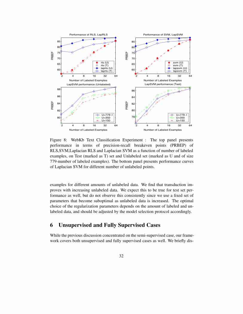
In the next experiment, we randomly split the webkb data into a test set of263 examples and a training set of 779 examples. We noted the performance ofinductive and semi-supervised classifiers on unlabeled and test sets as a function ofthe number of labeled examples in the training set. The performance measure is theprecision-recall breakeven point (PRBEP), averaged over 100 random data splits.Results are presented in the top panel of Figure 8. The benefit of unlabeled datacan be seen by comparing the performance curves of inductive and semi-supervisedclassifiers.

We also performed experiments with different sizes of the training set, keep-ing a randomly chosen test set of 263 examples. The bottom panel in Figure 8presents the quality of transduction and semi-supervised learning with LaplacianSVM (Laplacian RLS performed similarly) as a function of the number of labeled

31

2 4 8 16 32 64

60

65

70

75

80

85


PRBE

P

Performance of RLS, LapRLS

2 4 8 16 32 64

60

65

70

75

80

85


PRBE

P

Performance of SVM, LapSVM

2 4 8 16 32 64

80

82

84

86

88


PRBE

P

LapSVM performance (Unlabeled)

2 4 8 16 32 64

78

80

82

84

86

Number of Labeled ExamplesPR

BEP

LapSVM performance (Test)

rls (U)rls (T)laprls (U)laprls (T)

svm (U)svm (T)lapsvm (U)lapsvm (T)

U=779−lU=350U=150

U=779−lU=350U=150

Figure 8: WebKb Text Classification Experiment : The top panel presentsperformance in terms of precision-recall breakeven points (PRBEP) ofRLS,SVM,Laplacian RLS and Laplacian SVM as a function of number of labeledexamples, on Test (marked as T) set and Unlabeled set (marked as U and of size779-number of labeled examples). The bottom panel presents performance curvesof Laplacian SVM for different number of unlabeled points.

examples for different amounts of unlabeled data. We find that transduction im-proves with increasing unlabeled data. We expect this to be true for test set per-formance as well, but do not observe this consistently since we use a fixed set ofparameters that become suboptimal as unlabeled data is increased. The optimalchoice of the regularization parameters depends on the amount of labeled and un-labeled data, and should be adjusted by the model selection protocol accordingly.

6 Unsupervised and Fully Supervised Cases

While the previous discussion concentrated on the semi-supervised case, our frame-work covers both unsupervised and fully supervised cases as well. We briefly dis-

32

cuss each in turn.

6.1 Unsupervised Learning: Clustering and Data Representation

In the unsupervised case one is given a collection of unlabeled data points �� .Our basic algorithmic framework embodied in the optimization problem in Eqn. 3has three terms: (i) fit to labeled data, (ii) extrinsic regularization and (iii) intrin-sic regularization. Since no labeled data is available, the first term does not ariseanymore. Therefore we are left with the following optimization problem:

��

�� (26)

Of course, only the ratio �� matters. As before �� can be approximated using the

unlabeled data. Choosing �� and approximating it

by the empirical Laplacian, we are left with the following optimization problem:

� � ��

��

��

��

��

�� (27)

Note that to avoid degenerate solutions we need to impose some additional condi-tions (cf. [5]). It turns out that a version of Representer theorem still holds showingthat the solution to Eqn. 27 admits a representation of the form

� ��

��

By substituting back in Eqn. 27, we come up with the following optimization prob-lem:

� � ��

��

��

��

where � is the vector of all ones and � � �� and � is the correspondingGram matrix.

Letting � be the projection onto the subspace of � orthogonal to ��, oneobtains the solution for the constrained quadratic problem, which is given by thegeneralized eigenvalue problem

� �� (28)

The final solution is given by � � ��, where � is the eigenvector correspondingto the smallest eigenvalue.

33

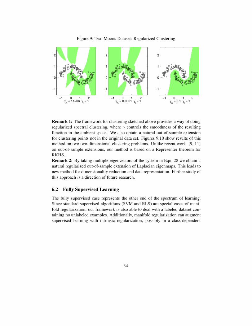
Figure 9: Two Moons Dataset: Regularized Clustering

−1 0 1 2

−1

0

1

2

γA = 1e−06 γ

I = 1

−1 0 1 2

−1

0

1

2

γA = 0.0001 γ

I = 1

−1 0 1 2

−1

0

1

2

γA = 0.1 γ

I = 1

Remark 1: The framework for clustering sketched above provides a way of doingregularized spectral clustering, where � controls the smoothness of the resultingfunction in the ambient space. We also obtain a natural out-of-sample extensionfor clustering points not in the original data set. Figures 9,10 show results of thismethod on two two-dimensional clustering problems. Unlike recent work [9, 11]on out-of-sample extensions, our method is based on a Representer theorem forRKHS.Remark 2: By taking multiple eigenvectors of the system in Eqn. 28 we obtain anatural regularized out-of-sample extension of Laplacian eigenmaps. This leads tonew method for dimensionality reduction and data representation. Further study ofthis approach is a direction of future research.

6.2 Fully Supervised Learning

The fully supervised case represents the other end of the spectrum of learning.Since standard supervised algorithms (SVM and RLS) are special cases of mani-fold regularization, our framework is also able to deal with a labeled dataset con-taining no unlabeled examples. Additionally, manifold regularization can augmentsupervised learning with intrinsic regularization, possibly in a class-dependent

34

Figure 10: Two Spirals Dataset: Regularized Clustering

−1 0 1

−1

−0.5

0

0.5

1

1.5

γA = 1e−06 γ

I = 1

−1 0 1

−1

−0.5

0

0.5

1

1.5

γA = 0.001 γ

I = 1

−1 0 1

−1

−0.5

0

0.5

1

1.5

γA = 0.1 γ

I = 1

manner, which suggests the following algorithm :

� � ��

�

�

��

��

��

��

��

�� (29)

Here we introduce two intrinsic regularization parameters �� , �� and regularizeseparately for the two classes : ��, �� are the vectors of evaluations of the function , and ��, �� are the graph Laplacians, on positive and negative examples respec-tively. The solution to the above problem for RLS and SVM can be obtained by

replacing �� by the block-diagonal matrix

��

� ��

�in the manifold

regularization formulae given in Section 4.Detailed experimental study of this approach to supervised learning is left for

future work.

7 Conclusions and Further Directions

We have a provided a novel framework for data-dependent geometric regulariza-tion. It is based on a new Representer theorem that provides a basis for severalalgorithms for unsupervised, semi-supervised and fully supervised learning. Thisframework brings together ideas from the theory of regularization in ReproducingKernel Hilbert spaces, manifold learning and spectral methods.

35

There are several directions of future research:1. Convergence and generalization error: The crucial issue of dependence ofgeneralization error on the number of labeled and unlabeled examples is still verypoorly understood. Some very preliminary steps in that direction have been takenin [6].2. Model selection: Model selection involves choosing appropriate values for theextrinsic and intrinsic regularization parameters. We do not as yet have a goodunderstanding of how to choose these parameters. More systematic proceduresneed to be developed.3. Efficient algorithms: It is worth noting that naive implementations of our opti-mization algorithms give rise to cubic time complexities, which might be imprac-tical for large problems. Efficient algorithms for exact or approximate solutionsneed to be devised.4. Additional structure: In this paper we have shown how to incorporate thegeometric structure of the marginal distribution into the regularization framework.We believe that this framework will extend to other structures that may constrainthe learning task and bring about effective learnability. One important example ofsuch structure is invariance under certain classes of natural transformations, suchas invariance under lighting conditions in vision.

Acknowledgments

We are grateful to Marc Coram, Steve Smale and Peter Bickel for intellectual sup-port and to NSF funding for financial support. We would like to acknowledge theToyota Technological Institute for its support for this work.

References

[1] R. A. Adams, Sobolev Spaces, Academic Press, New York, 1975.

[2] N. Aronszajn, Theory of Reproducing Kernels, Transactions of the American athe-matical Society, Vol. 68, Issue 3, p337-404, 1950.

[3] M. Belkin, Problems of Learning on Manifolds, The University of Chicago, Ph.D.Dissertation, 2003.

[4] M. Belkin, P. Niyogi, Using Manifold Structure for Partially Labeled Classification,NIPS 2002.

[5] M. Belkin, P. Niyogi. (2003). Laplacian Eigenmaps for Dimensionality Reductionand Data Representation, Neural Computation, Vol. 15, No. 6, 1373-1396.

36

[6] M. Belkin, I. Matveeva, P. Niyogi, Regression and Regularization on Large Graphs,COLT 2004.

[7] O. Bousquet, O. Chapelle, M. Hein, Measure Based Regularization, NIPS 2003.

[8] Y. Bengio, O. Delalleau and N.Le Roux, Efficient Non-Parametric Function Induc-tion in Semi-Supervised Learning, Technical Report 1247, DIRO, University of Mon-treal, 2004.

[9] Y. Bengio, J-F. Paiement, and P. Vincent,Out-of-Sample Extensions for LLE, Isomap,MDS, Eigenmaps, and Spectral Clustering, NIPS 2003.

[10] K. Bennett and A. Demirez, Semi-Supervised Support Vector Machines, Advances inNeural Information Processing Systems, 12, M. S. Kearns, S. A. Solla, D. A. Cohn,editors, MIT Press, Cambridge, MA, 1998, pp 368-374

[11] M. Brand, Nonlinear dimensionality reduction by kernel eigenmaps. Proceedings ofthe Eighteenth International Joint Conference on Artificial Intelligence, pp. 547-552,Acapulco, Mexico, 9-15 August 2003.

[12] A. Blum, S. Chawla, Learning from Labeled and Unlabeled Data using Graph Min-cuts, ICML 2001.

[13] A. Blum, T. Mitchell, Combining Labeled and Unlabeled Data with Co-Training,Proceedings of the 11th Annual Conference on Computational Learning Theory,pages 92–100, 1998

[14] Chapelle, O., J. Weston and B. Schoelkopf, Cluster Kernels for Semi-SupervisedLearning, NIPS 2002.

[15] F. R. K. Chung. (1997). Spectral Graph Theory. Regional Conference Series in Math-ematics, number 92.

[16] A. Corduneanu, T.Jaakkola, On Information Regularization, UAI 2003.

[17] F. Cucker, S. Smale, On the Mathematical Foundations of Learning, Bull. Amer.Math. Soc. 39 (2002), 1-49.

[18] S. T. Dumais, J. Platt, D. Heckerman and M. Sahami (1998).Inductive learning algo-rithms and representations for text categorization, In Proceedings of ACM-CIKM98,Nov. 1998, pp. 148-155

[19] D. L. Donoho, C. E. Grimes, Hessian Eigenmaps: new locally linear embedding tech-niques for high-dimensional data, Proceedings of the National Academy of Arts andSciences vol. 100 pp. 5591-5596.

[20] T. Evgeniou, M. Pontil and T. Poggio, Regularization Networks and Support VectorMachines, Advances in Computational Mathematics, Vol. 13, 1-50, 2000.

[21] G. Fung and O. L. Mangasarian, Semi-Supervised Support Vector Machines for Un-labeled Data Classification, Optimization Methods and Software 15, 2001, 29-44

[22] T. Joachims, Transductive Inference for Text Classification using Support Vector Ma-chines, ICML 1999.

37

[23] T. Joachims, Transductive Learning via Spectral Graph Partitioning, Proceedings ofthe International Conference on Machine Learning (ICML), 2003

[24] C.C. Kemp, T.L. Griffiths, S. Stromsten, J.B. Tenenbaum, Semi-supervised Learningwith Trees, NIPS 2003.

[25] K. Nigam, A. McCallum, S. Thrun and T. Mitchell. Text Classification from Labeledand Unlabeled Documents using EM. Machine Learning, 39(2/3). pp. 103-134. 2000.

[26] R. Rifkin, Everything Old Is New Again: A Fresh Look at Historical Approaches inMachine Learning, PhD Thesis, MIT, 2002.

[27] Sam T. Roweis, Lawrence K. Saul. (2000). Nonlinear Dimensionality Reduction byLocally Linear Embedding, Science, vol 290.

[28] M. Seeger Learning with Labeled and Unlabeled Data, Technical Report. EdinburghUniversity (2000)

[29] A. Smola and R. Kondor, Kernels and Regularization on Graphs, COLT/KW 2003.

[30] B. Schoelkopf, C.J.C. Burges, V. Vapnik, Extracting Support Data for a Given Task,KDD95.

[31] B. Schoelkopf, A. Smola, Learning with Kernels, 644, MIT Press, Cambridge, MA(2002).

[32] Martin Szummer, Tommi Jaakkola, Partially labeled classification with Markov ran-dom walks, NIPS 2001.

[33] J.B.Tenenbaum, V. de Silva, J. C. Langford. (2000). A Global Geometric Frameworkfor Nonlinear Dimensionality Reduction, Science, Vol 290.

[34] A.N. Tikhonov, Regularization of Incorrectly Posed Problems, Soviet Math. Doklady4, 1963 (English Translation).

[35] V. Vapnik, Statistical Learning Theory, Wiley-Interscience, 1998.

[36] G. Wahba. (1990). Spline Models for Observational Data, Society for Industrial andApplied Mathematics.

[37] D. Zhou, O. Bousquet, T.N. Lal, J. Weston and B. Schoelkopf, Learning with Localand Global Consistency, NIPS 2003.

[38] X. Zhu, J. Lafferty and Z. Ghahramani, Semi-supervised learning using Gaussianfields and harmonic functions, ICML 2003.

[39] http://www.cse.msu.edu/�lawhiu/manifold/

38