manifold representations for state estimation in contact ... · manifold representations for state...

Manifold Representations for State Estimationin Contact Manipulation

Michael C. Koval, Nancy S. Pollard, and Siddhartha S. Srinivasa

Abstract We investigate the problem of using contact sensors to estimate the con-figuration of an object during manipulation. Contact sensing is very discriminativeby nature and, therefore, the set of object configurations that a sensor constitutesa lower-dimensional manifold in the state space of the object. This causes conven-tional state estimation methods, such as particle filters, to perform poorly duringperiods of contact. The manifold particle filter addresses this problem by samplingparticles directly from the contact manifold. When it exists, we can sample theseparticles from an analytic representation of the contact manifold. We present two al-ternative sample-based contact manifold representations that make no assumptionsabout the object-hand geometry: rejection sampling and trajectory rollouts. The re-jection sampling representation distributes uniformly in the space surrounding themanifold, while the trajectory rollout representation concentrates samples on the re-gions of the manifold that we are most likely to encounter during execution. Wediscuss theoretical considerations behind these three representations and comparetheir performance in an extensive suite of simulation experiments. We show that allthree representations enable the manifold particle filter to outperform the conven-tional particle filter. Additionally, we show that the trajectory rollout representationperforms similarly to the analytic method despite its relative simplicity.

1 Introduction

Humans effortlessly use their sense of touch to manipulate objects. Imagine gropingaround on a nightstand for a glass of water, or feeling around a cluttered kitchencabinet while searching for the salt shaker. Each of these tasks involves contact

manipulation where we make persistent contact with the environment. Our contactobservations are critical for localizing the object as we manipulate it.

Michael C. Koval, Nancy S. Pollard, Siddhartha S. SrinivasaRobotics Institute, Carnegie Mellon Universitye-mail: {mkoval,nsp,siddh}@cs.cmu.edu

1

2 Michael C. Koval, Nancy S. Pollard, and Siddhartha S. Srinivasa

Fig. 1: HERB is pushing a rectangular box across the table. The state x ∈ X is thepose of the box relative to the hand. An action u ∈ U is a relative motion of thehand. After taking action u, HERB receives an observation z ∈ Z indicating wherethe object touched the hand.

Armed with real-time observations from tactile sensors [Odhner et al., 2013,Tenzer et al., 2012, Fishel & Loeb, 2012], manipulators should be also able to es-timate the state of the manipulated object—a problem we formalize as the state

estimation for contact manipulation problem (Section 2).Early work attempted to solve this problem by deriving analytical state estimators

and controllers to track and control the pose of an object from contact positionsbased on simple models of physics [Jia & Erdmann, 1999]. These models fail toaccurately capture the reality of manipulation: there is a large amount of uncertaintyin both the object’s motion and the robot’s observations.

Other work has employed a Bayesian approach by using the particle filter to esti-mate the pose [Zhang & Trinkle, 2012] and physical properties [Zhang et al., 2013]of an object during manipulation. However, our prior work [Koval et al., 2013] re-vealed that the conventional particle filter (CPF) performs poorly at real-time updaterates and suffers from a startling problem: the CPF systematically performs worse

as sensor resolution increases (Section 3).This problem arises because contact sensing accurately discriminates between

contact and no-contact. Topologically, the set of object configurations that agreewith a contact observation lies in the lower dimensional observable contact mani-

fold embedded in the configuration space of the object (Section 2). Particles sampledfrom the state space during contact have low probability of falling into the obser-vation space. This results in particle starvation in the vicinity of the true state. Themanifold particle filter (MPF) provides a principled way of solving this problem bysampling particles directly from the observable contact manifold (Section 4).

Applying the MPF to the state estimation for contact manipulation problem re-quires sampling particles from the observable contact manifold. When it exists, ananalytic representation (AM) of the manifold provides an exact and computationallyefficient way of sampling from the dual proposal distribution (Section 5). However,computing an analytic representation of the contact manifold is not always possible.

We present two alternative sample-based contact manifold representations thatmake no assumptions about the object-hand geometry: rejection sampling (RS) andtrajectory rollouts (TR). The RS representation distributes samples uniformly in thespace surrounding the manifold, while the TR representation concentrates many

Manifold Representations for State Estimation in Contact Manipulation 3

samples on the regions of the manifold that we are most likely to encounter duringexecution (Section 6).

Our results (Section 6) reveal the tradeoffs between these representations. RSperforms the worst. By distributing samples uniformly everywhere, even in unlikelyregions, RS is relatively sparse everywhere. Surprisingly, TR performed nearly aswell as AM. By focusing samples on likely regions, TR was able to saturate thoseregions at a resolution that was indistinguishable from AM. A key reason is thatlikely regions occupy only a small portion of the contact manifold in our experi-ments, where the hand pushes straight towards the object.

Our key takeaway is to exploit structure. By exploiting the manifold structureof the contact state estimation problem, we are able to outperform the CPF. Fur-thermore, by exploiting the geometry of the hand-object interaction with trajectoryrollouts, we are able to perform as well as the analytical method.

We are excited by our future directions. First, in generalizing state to materialproperties, and even shape, enabling us to simultaneously estimate shape and posefrom contact. Second, in closing the loop between state estimation and control, todevelop robust closed-loop policies for contact manipulation.

2 State Estimation for Contact Manipulation

Let x ∈ X be the state of a dynamical system which evolves over time under actionsu ∈U and produces observations z ∈ Z. The state estimation problem addresses thecomputation of the belief state, a probability distribution over the current state xt

given the past history of actions u1:t and observations z1:t :

b(xt) = p(xt |z1:t ,u1:t) (1)

We focus on the state estimation for contact manipulation problem, where thestate is the pose x (Fig. 1-Left) of the manipulated object and an action u (Fig. 1-Middle) is a relative motion of the hand. During contact the object moves accordingto the stochastic transition model p(xt |xt−1,ut) that encodes the physics of the ob-ject’s motion in response to pushing action ut . The stochasticity of the transitionmodel may be due to unknown physical properties of the object (e.g. friction coeffi-cients), imperfections in the physics simulation, or error in executing ut .

Contact sensors attached to the surface of the hand provide observations zt

(Fig. 1-Right) that indicate whether the object is touching the sensor. This is equiv-alent to testing whether xt ∈ Xo, where Xo ⊆ X is the set of states where the objectis in contact with one or more sensors. While x ∈ Xo, zt may provide additional in-formation about the configuration of the object through noisy measurement of itscontact with the hand. Both of these properties are combined into the stochastic ob-

servation model p(zt |xt ,ut) as the probability of state xt generating observation zt

after executing action ut .The Contact Manifold. The key challenge for state estimation arises because stateevolves on a lower-dimensional contact manifold. We can partition X into three partsdepending upon the type of contact occurring between the hand and the object: (1)penetrating contact Xpen, (2) non-penetrating contact Xc, and (3) no contact X f ree.


x y

θ

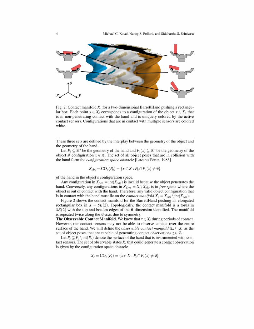
Fig. 2: Contact manifold Xc for a two-dimensional BarrettHand pushing a rectangu-lar box. Each point x ∈ Xc corresponds to a configuration of the object x ∈ Xc thatis in non-penetrating contact with the hand and is uniquely colored by the activecontact sensors. Configurations that are in contact with multiple sensors are coloredwhite.

These three sets are defined by the interplay between the geometry of the object andthe geometry of the hand.

Let Ph ⊆ Rn be the geometry of the hand and Po(x)⊆ R

n be the geometry of theobject at configuration x ∈ X . The set of all object poses that are in collision withthe hand form the configuration space obstacle [Lozano-Perez, 1983]

Xobs = COo(Ph) = {x ∈ X : Ph∩Po(x) 6= /0}

of the hand in the object’s configuration space.Any configuration in Xpen = int(Xobs) is invalid because the object penetrates the

hand. Conversely, any configurations in X f ree = X \Xobs is in free space where theobject is out of contact with the hand. Therefore, any valid object configuration thatis in contact with the hand must lie on the contact manifold Xc = Xobs \ int(Xobs).

Figure 2 shows the contact manifold for the BarrettHand pushing an elongatedrectangular box in X = SE(2). Topologically, the contact manifold is a torus inSE(2) with the top and bottom edges of the θ -dimension identified. The manifoldis repeated twice along the θ -axis due to symmetry.The Observable Contact Manifold. We know that x∈Xc during periods of contact.However, our contact sensors may not be able to observe contact over the entiresurface of the hand. We will define the observable contact manifold Xo ⊆ Xc as theset of object poses that are capable of generating contact observations z ∈ Zc.

Let Ps ⊆ Po \ int(Po) denote the surface of the hand that is instrumented with con-tact sensors. The set of observable states Xs that could generate a contact observationis given by the configuration space obstacle

Xs = COo(Ps) = {x ∈ X : Ps∩Po(x) 6= /0}


of the sensor in the object’s configuration space. The observable contact manifold

Xo = Xs∩Xc consists of the set of valid object configurations that have high proba-bility of generating a contact observation z ∈ Zc.

Figure 2 shows the contact manifold colored by which sensors are active at eachpoint. Any state in the large, dark orange region of the manifold are in contactwith—and, thus, will stimulate, the left distal contact sensor. States in the largewhite region of the manifold are simultaneously in contact with multiple sensors.Discriminative Observation Model. Contact sensors accurately discriminate be-tween contact and no-contact. We call an observation model discriminative if wecan partition the set of observations Z into sets of contact Zc ⊆ Z and no-contactZnc = Z \Zc observations such that there are few false-positive and false-negative in-dications of contact. Therefore, a discriminative observation model satisfies Pr(z ∈Zc|x ∈ Xo,u) > 1− ε during periods of contact and Pr(z ∈ Znc|x 6∈ Xo,u) > 1− εduring no-contact.

3 Conventional Particle Filter

The Bayes filter is the most general algorithm for filtering a belief state given asequence of actions and observations by recursively constructs b(xt) from b(xt−1)using the update rule

b(xt) = η p(zt |xt ,ut)∫

Xp(xt |xt−1,ut)b(xt−1)dxt−1 (2)

where η is a normalization factor. The terms p(zt |xt ,ut) and p(xt |xt−1,ut) are, re-spectively, the observation and transition models. The recursion is initialized witha prior belief b(x0) provided by task-specific knowledge or other sensors (e.g. anobject recognition system).

The particle filter [Thrun et al., 2005] is a non-parametric formulation of theBayes filter that represents the belief state b(xt) with a discrete set of samples. The

samples Xt = {x[i]t }

ni=1 are called particles and are distributed according to the belief

state x[i]t ∼ b(xt). The particle filter implements the Bayesian update (Eq. 2) by re-

cursively constructing Xt from Xt−1 using a technique called importance sampling.The conventional particle filter (CPF) is summarized in algorithm 1. The key

insight behind this realization is that it is difficult to directly sample from the tar-

get distribution (Eq. 2), but it is relatively easy to sample from the transition model.

Therefore, we sample x[i]t from the proposal distribution

∫

X p(xt |xt−1,ut)b(xt−1)dxt−1

(line 3) by forward-simulating Xt−1 to Xt using the motion model. Next, we compute

an importance weight w[i]t = p(zt |xt ,ut) for each forward-simulated particle (line 4).

The importance weights result from dividing the target distribution by the pro-

posal distribution. As a result, the samples x[i]t , along with their importance weights

w[i]t , are distributed according to the target distribution b(xt). Intuitively, the weight-

ing step incorporates the observation model into the update by assigning higherweight to particles that are consistent with zt .


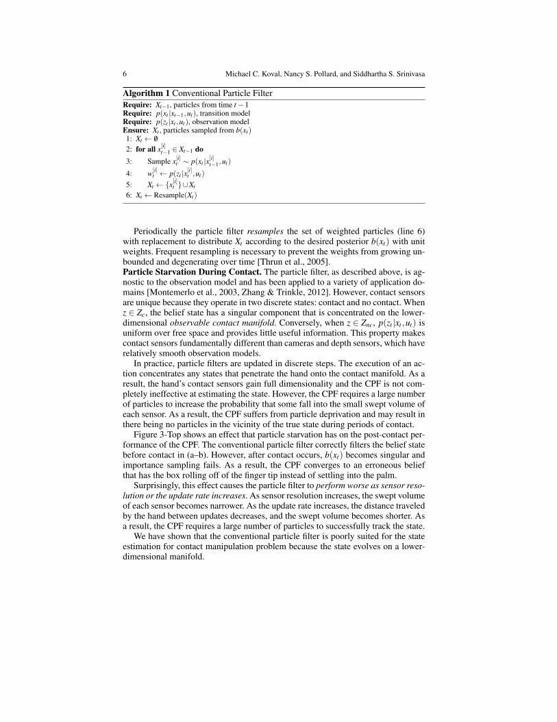
Algorithm 1 Conventional Particle Filter

Require: Xt−1, particles from time t−1Require: p(xt |xt−1,ut), transition modelRequire: p(zt |xt ,ut), observation modelEnsure: Xt , particles sampled from b(xt)1: Xt ← /0

2: for all x[i]t−1 ∈ Xt−1 do

3: Sample x[i]t ∼ p(xt |x

[i]t−1,ut)

4: w[i]t ← p(zt |x

[i]t ,ut)

5: Xt ←{x[i]t }∪Xt

6: Xt ← Resample(Xt)

Periodically the particle filter resamples the set of weighted particles (line 6)with replacement to distribute Xt according to the desired posterior b(xt) with unitweights. Frequent resampling is necessary to prevent the weights from growing un-bounded and degenerating over time [Thrun et al., 2005].Particle Starvation During Contact. The particle filter, as described above, is ag-nostic to the observation model and has been applied to a variety of application do-mains [Montemerlo et al., 2003, Zhang & Trinkle, 2012]. However, contact sensorsare unique because they operate in two discrete states: contact and no contact. Whenz ∈ Zc, the belief state has a singular component that is concentrated on the lower-dimensional observable contact manifold. Conversely, when z ∈ Znc, p(zt |xt ,ut) isuniform over free space and provides little useful information. This property makescontact sensors fundamentally different than cameras and depth sensors, which haverelatively smooth observation models.

In practice, particle filters are updated in discrete steps. The execution of an ac-tion concentrates any states that penetrate the hand onto the contact manifold. As aresult, the hand’s contact sensors gain full dimensionality and the CPF is not com-pletely ineffective at estimating the state. However, the CPF requires a large numberof particles to increase the probability that some fall into the small swept volume ofeach sensor. As a result, the CPF suffers from particle deprivation and may result inthere being no particles in the vicinity of the true state during periods of contact.

Figure 3-Top shows an effect that particle starvation has on the post-contact per-formance of the CPF. The conventional particle filter correctly filters the belief statebefore contact in (a–b). However, after contact occurs, b(xt) becomes singular andimportance sampling fails. As a result, the CPF converges to an erroneous beliefthat has the box rolling off of the finger tip instead of settling into the palm.

Surprisingly, this effect causes the particle filter to perform worse as sensor reso-

lution or the update rate increases. As sensor resolution increases, the swept volumeof each sensor becomes narrower. As the update rate increases, the distance traveledby the hand between updates decreases, and the swept volume becomes shorter. Asa result, the CPF requires a large number of particles to successfully track the state.

We have shown that the conventional particle filter is poorly suited for the stateestimation for contact manipulation problem because the state evolves on a lower-dimensional manifold.


Algorithm 2 Manifold Particle Filter

Require: Xt−1, particles from time t−1Require: k, number of dual particles to sampleEnsure: Xt , particles sampled from b(xt)1: XMi

← /0 for i = 1, . . . ,m2: for 1, . . . ,k do3: Sample Mi ∼ Pr(xt ∈Mi)4: if Mi 6= Mm then

5: Sample x[i]t ∼ p(zt |Mi,xt ,ut)/p(zt |Mi,ut)

6: w[i]t ← ·EstimateDensity(Xt−1,ut , x

[i]t )

7: XMi←{x

[i]t }∪ XMi

8: end if9: XMm ← ConventionalProposal(Xt−1,ut ,zt)∩Mm

10: Xt ← Resample(∑mi=1 Pr(xt ∈Mi)XMi

)

4 Manifold Particle Filter

Suppose the state space X is partitioned into m disjoint components M = {Mi}mi=1,

where M1, . . . ,Mm−1 ⊆ X are manifolds and Mm = X \∪m−1i=1 Mi is the remaining free

space. The belief state b(x) may have a singular component with non-zero probabil-

ity concentrated on the lower-dimensional manifolds {Mi}m−1i=1 .

We redefine the belief state as the weighted sum

b(xt) = ∑Mi∈M

b(xt |Mi)Pr(xt ∈Mi) (3)

over manifolds, where b(xt |Mi) is the belief over Mi given that xt ∈Mi.1

The manifold particle filter (MPF), summarized in algorithm 2, also representsthe belief using particles. For each particle, we first choose which manifold to sam-

ple from according to Mi ∼ Pr(xt ∈Mi). Then, we sample the particle x[i]t ∼ b(xt |Mi)

from the corresponding conditional belief using a sampling technique that is appro-priate for the structure of Mi.

Ideally, we could compute Pr(xt ∈Mi) by marginalizing over Mi. Unfortunately,this is fundamentally impossible for two reasons. First, marginalizing requires b(xt),precisely the distribution that we are trying to estimate. Second,

∫

Mib(xt)dxt = 0

because Mi is a measure zero set.Instead, we approximate Pr(xt ∈Mi) using only the most recent observation

Pr(xt ∈Mi)≈p(zt |Mi,ut)

p(zt |ut)(4)

where p(zt |Mi,ut) is the probability that zt was generated by a an xi ∈ Mi andp(zt |ut) =

∫

X p(zt |xt ,ut)dxt is the prior probability of receiving observation zt . How-ever, Eq. 4 is a good approximation in the case where p(zt |xt ,ut) accurately discrim-inates between manifolds.

1 From this point forward we will use b(xt) as shorthand for the weighted sum in Eq. 3.


Finally, we can sample a particle x[i]t according to the belief distribution over the

chosen manifold b(xt |Mi). Our key insight is that we can apply a different samplingtechnique for each Mi that is specifically designed to take advantage of the structureof the manifold. For the manifolds {Mi}

m−1i=1 , we sample from the dual proposal

distribution [Thrun et al., 2000] as described below. In the case of the free space Mm,

we sample x[i]t with the conventional technique and reject any x

[i]t ∈ ∪

m−1i=1 Mi. This

rejection sampling step is necessary to avoid biasing the estimate of b(xt) towardsthe manifolds.Dual Proposal Distribution. Importance sampling from the conventional proposaldistribution fails on Mi for i < m because they are lower-dimensional manifolds. Inthis case, we will sample from the dual proposal distribution [Thrun et al., 2000]

x[i]t ∼ η

p(zt |Mi,xt ,ut)

p(zt |Mi,ut), (5)

where η is a normalization constant. We can find the corresponding importanceweights

w[i]t =

∫

Mi

p(x[i]t |xt−1,ut)b(xt−1|Mi)dxt−1. (6)

by dividing the target distribution (Eq. 2) by the proposal distribution (Eq. 5).The conventional proposal distribution forward-predicts using the motion model

and computes importance weights using the observation model. Conversely, thedual proposal distribution samples particles from the observation model and weightsthem by how well they agree with the motion model. [Thrun et al., 2000].Mixture Proposal Distribution. Just as how the conventional proposal distribu-tion performs poorly with accurate sensors, the dual proposal distribution performspoorly when there is observation noise. The MPF uses the dual proposal distributionto sample from the manifolds and, as result, shares the same weakness.

We use a mixture proposal distribution [Thrun et al., 2000] to mitigate this effectby combining both sampling techniques. Instead of sampling all of the particlesfrom the MPF, we sample n particles from the CPF and d particles from the MPF. Wethen combine the two sets of particles with the weighted sum (1−φ)Xt +φ Xt beforeresampling. The mixing rate 0 ≤ φ ≤ 1 is a parameter that allows the algorithm tosmoothly transition from the CPF (φ = 0) to the MPF (φ = 1).

Intuitively, d = |Xt | is the number of particles necessary to simultaneously coverall of the manifolds and n = |Xt | is the number of additional particles necessary torepresent b(xt) in free space.

5 Manifold Particle Filter for Contact Manipulation

In this section, we will apply the MPF to the state estimation for contact manip-ulation problem. To do so, we will define the observable contact manifold Xo andfree space X f ree as the relevant subsets of X . We will also describe a technique for

computing the importance weights w[i]i using kernel density estimation.


CP

FM

PF

b(x

t)M

PF

b(x

t|X

o)

(a) Prior Belief (b) Pre-Contact (c) Post-Contact (d) Final Belief

Fig. 3: Snapshots of the MPF during execution. Unlike the CPF, the MPF explicitlytracks the probability distribution on the contact manifold Xc.

Figure 3 shows the performance of the MPF relative to the CPF. Before contact(a–b), Pr(xt ∈ Xo) ≈ 0 and both filters update using the conventional proposal dis-tribution. After contact (c–d), Pr(xt ∈ Xo)≈ 1 and the manifold particle filter beginssampling from Xo. Sampling from the observable contact manifold allows the MPFto accurately track the object’s pose during persistent contact.Importance Sampling from the Contact Manifold. We must weight the sam-ples drawn from the dual proposal distribution with their corresponding importance

weights w[i] =∫

X p(xt |xt−1,ut)b(xt−1)dxt−1. Intuitively, this integrates our beliefstate b(xt−1) prior to taking action ut into b(xt).

We evaluate w[i] by forward-simulating the previous set of particles Xt−1 to timet by sampling from p(xt |xt−1,ut), then evaluating the density of the distribution

at x[i]t using a density estimation technique [Thrun et al., 2000]. Ideally, we would

compute a density estimate over the manifold Xo. Unfortunately, while there hasbeen some work on density estimation on Riemannian manifolds [Pelletier, 2005],but it is difficult to apply these algorithms to the approximate and sample-basedrepresentations of Xo described below. This is exacerbated by the fact that many ofour forward-simulated particles will not lie on Xo.

Instead, we use kernel density estimation to approximate the probability densityover X , then restrict the estimate to Xo ⊂ X . Figure 3 shows an example of the re-sulting density estimate over X f ree (Fig. 3-Middle) and Xo (Fig. 3-Bottom) computedusing Gaussian kernels with bandwidths selected by Silverman’s rule of thumb.


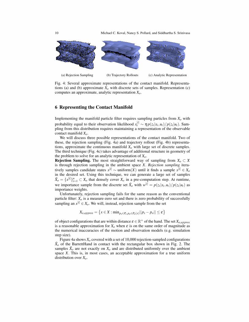
(a) Rejection Sampling (b) Trajectory Rollouts (c) Analytic Representation

Fig. 4: Several approximate representations of the contact manifold. Representa-tions (a) and (b) approximate Xo with discrete sets of samples. Representation (c)computes an approximate, analytic representation Xo.

6 Representing the Contact Manifold

Implementing the manifold particle filter requires sampling particles from Xo with

probability equal to their observation likelihood x[i]t ∼ η p(zt |xt ,ut)/p(zt |ut). Sam-

pling from this distribution requires maintaining a representation of the observablecontact manifold Xo.

We will discuss three possible representations of the contact manifold. Two ofthese, the rejection sampling (Fig. 4a) and trajectory rollout (Fig. 4b) representa-tions, approximate the continuous manifold Xo with large set of discrete samples.The third technique (Fig. 4c) takes advantage of additional structure in geometry ofthe problem to solve for an analytic representation of Xo.Rejection Sampling. The most straightforward way of sampling from Xo ⊂ X

is through rejection sampling in the ambient space X . Rejection sampling itera-

tively samples candidate states x[i] ∼ uniform(X) until it finds a sample x[i] ∈ Xo

in the desired set. Using this technique, we can generate a large set of samples

Xo = {x[i]}ni=1 ⊂ Xo that densely cover Xo in a pre-computation step. At runtime,

we importance sample from the discrete set Xo with w[i] = p(zt |xt ,ut)/p(zt |ut) asimportance weights.

Unfortunately, rejection sampling fails for the same reason as the conventionalparticle filter: Xo is a measure-zero set and there is zero probability of successfully

sampling an x[i] ∈ Xo. We will, instead, rejection sample from the set

Xo,approx ={

x ∈ X : minps∈Ps,po∈Po(x)||ps− po|| ≤ ε}

of object configurations that are within distance ε ∈R+ of the hand. The set Xo,approx

is a reasonable approximation for Xo when ε is on the same order of magnitude asthe numerical inaccuracies of the motion and observation models (e.g. simulationstep size).

Figure 4a shows Xo covered with a set of 10,000 rejection-sampled configurationsXo of the BarrettHand in contact with the rectangular box shown in Fig. 2. Thesamples Xo are not exactly on Xo and are distributed uniformly over the ambientspace X . This is, in most cases, an acceptable approximation for a true uniformdistribution over Xo.


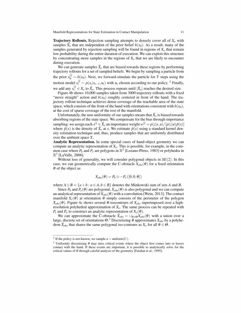
Trajectory Rollouts. Rejection sampling attempts to densely cover all of Xo withsamples Xo that are independent of the prior belief b(x0). As a result, many of thesamples generated by rejection sampling will be found in regions of Xo that remainlow probability during the entire duration of execution. We can exploit this structureby concentrating more samples in the regions of Xo that we are likely to encounterduring execution.

We can generate samples Xo that are biased towards these regions by performingtrajectory rollouts for a set of sampled beliefs. We begin by sampling a particle from

the prior x[i]0 ∼ b(x0). Next, we forward-simulate the particle for T steps using the

motion model x[i]t ∼ p(xt |xt−1,ut) with ut chosen according to our policy. 2 Finally,

we add any x[i]t ∈ Xo to Xo. This process repeats until |Xo| reaches the desired size.

Figure 4b shows 10,000 samples taken from 3000 trajectory rollouts with a fixed“move straight” action and b(x0) roughly centered in front of the hand. The tra-jectory rollout technique achieves dense coverage of the reachable area of the statespace, which consists of the front of the hand with orientations consistent with b(x0),at the cost of sparse coverage of the rest of the manifold.

Unfortunately, the non-uniformity of our samples means that Xo is biased towardsabsorbing regions of the state space. We compensate for the bias through importance

sampling: we assign each x[i] ∈ Xo an importance weight w[i]= p(z|x,u)/[p(z|u)p(x)]where p(x) is the density of Xo at x. We estimate p(x) using a standard kernel den-sity estimation technique and, thus, produce samples that are uniformly distributedover the ambient space X .Analytic Representation. In some special cases of hand-object geometry we cancompute an analytic representation of Xo. This is possible, for example, in the com-mon case where Ph and Po are polygons in R

2 [Lozano-Perez, 1983] or polyhedra inR

3 [LaValle, 2006].Without loss of generality, we will consider polygonal objects in SE(2). In this

case, we can geometrically compute the C-obstacle Xobs(θ) for a fixed orientationθ of the object as

Xobs(θ) = Ph⊕−Po ([0,0,θ ])

where A⊕B = {a+b : a ∈ A,b ∈ B} denotes the Minkowski sum of sets A and B.Since Ph and Po(θ) are polygonal, Xobs(θ) is also polygonal and we can compute

an analytical representation of Xobs(θ) with a convolution [Wein, 2013]. The contactmanifold Xc(θ) at orientation θ simply consists of the perimeter of the polygonXobs(θ). Figure 4c shows several θ -isocontours of Xobs superimposed over a high-resolution polyhedral approximation of Xo. The same process can be repeated withPs and Po to construct an analytic representation of Xo(θ).

We can approximate the C-obstacle Xobs = ∪θ∈Θ Xobs(θ) with a union over alarge, discrete set of orientations Θ .3 Discretizing θ approximates Xobs by a polyhe-dron Xobs that shares the same polygonal iso-contours as Xo for all θ ∈Θ .

2 If the policy is not known, we sample u∼ uniform(U).3 Uniformly discretizing θ may miss critical events where the object first comes into or leavescontact with the hand. If these events are important, it is possible to analytically solve for thecritical values of θ through careful analysis of the geometry [Farahat et al., 1995].


Sampling an x[i] ∼ Xo is possible by first sampling a θ ∈Θ , then uniformly sam-

pling an x[i] from our analytical representation of Xo(θ). Alternatively, one couldsample from an approximate, polyhedral representation of Xo by interpolating be-tween iso-contours. In both cases, the samples are correctly drawn uniformly withrespect to a measure defined over the lower-dimensional Xo.

7 Experiments and Results

We designed a set of simulation experiments to compare the MPF with the CPF forthe state estimation for contact manipulation problem, and to explore the differencesbetween the three representations of the contact manifold.

Based on the particle starvation problem, we hypothesize that

H1. The MPF will outperform the CPF after contact.

Among the three representations of the contact manifold, we expect the rejectionsampling (RS) representation to perform the worst due to its relatively sparse dis-tribution of samples. The trajectory rollout (TR) representation solves this problemby concentrating samples on the regions of the contact manifold that we are mostlikely to encounter.

Therefore, we hypothesize:

H2. Trajectory rollouts will outperform rejection sampling.

H3. The analytic contact manifold will outperform rejection sampling.

However, we hypothesize that the analytic representation will outperform boththe RS and TR representations because it exactly represents the contact manifold:

H4. The analytic contact manifold will perform best.

7.1 Experimental Design

Setup. We implemented the CPF, MPF-RS, MPF-TR, and MPF-TR in a customtwo-dimensional kinematic simulation environment with polygonal geometry. Eachexperiment consisted of a simulated BarrettHand pushing a rectangular box in astraight line at a speed of 1 cm/s for 50 cm. The initial belief state was set to b(x0) =

N (0,Σ) with Σ 1/2 = diag[5 cm,5 cm,20◦].Motion Model. We simulated the motion of the object using a penetration-basedquasistatic physics simulator [Lynch et al., 1992] with a 1 mm step size. Duringeach update, the finger-object coefficient of friction µ and the radius of the ob-ject’s pressure distribution c were sampled from the Gaussian distributions µ ∼N(0.5,0.22) and c∼ N(0.05,0.012) truncated at µ,c > 0.Observation Model. Binary observations were simulated for each of the hand’ssensors by computing the intersection of the contact sensor with the object’s geom-etry. Ground-truth observations were simulated by applying the same observationmodel to a special “ground truth” particle sampled from b(x0).


0

2

4

6

8

10

RMSE

(cm)

CPF

MPF

-5 0 5 10 15

Time (s)

05

101520253035

RMSE

(◦)

(a) Manifold Particle Filter

0

2

4

6

8

10

RMSE

(cm)

RSTRAM

-5 0 5 10 15

Time (s)

05

101520253035

RMSE

(◦)

(b) Contact Manifold Representations

Fig. 5: (a) Estimation error of the CPF and MPF. (b) Performance of MPF usingthe rejection-sampled (RS), trajectory-rollout (TR), and analytical (AM) manifoldrepresentations. In both cases, the data is aligned such that contact occurs at t = 0.

Dependent Measure. We measure performance of the estimators by tracking theroot mean square error (RMSE) of the object’s position (Fig. 5a-Top) and orientation(Fig. 5a-Bottom) over a large number of experiments

7.2 Conventional vs. Manifold Particle Filter (H1)

Both the CPF and the MPF used 100 particles. The MPF used an analytic represen-tation of the contact manifold and a mixing rate of φ = 0.1

As expected, both filters behave similarly before contact (t ≤ 0) and there nota significant difference in RMSE. After contact (t > 0), the MPF quickly achieves4.4 cm less RMSE than the CPF. These results support hypothesis H1: the MPFachieves lower post-contact error than the CPF.

7.3 Contact Manifold Representation (H2–H4)

We also compared the RMSE error of the MPF using the rejection sampling (RS),trajectory rollouts (TR), and an analytic (AM) representations of the contact man-ifold. The RS representation consisted of 10,000 samples that were held constantthroughout all of the experiments. The TR representation generated a different set10,000 samples for each experiment by collecting five samples each from 2000 tra-jectory rollouts. Finally the AM representation was implemented by sampling frompolygonal iso-contours of Xo spaced every 3◦ of angular resolution.


All three implementations of the MPF outperformed the CPF. As expected, theAM and TR representations both outperformed the RS representation, supportinghypotheses H2 and H3. This occurs because the RS representation attempts tosparsely cover the entire surface Xo with a relatively small number of samples, whilethe TR representation densely covers the states that we are most likely to reach.

Surprisingly, hypothesis H4 was not supported by the data: the AM representa-tion did not achieve lower error than the TR representation. This occurred becausethe TR representation was able to saturate the regions of Xo that we are likely to en-counter during execution. By doing so, the TR representation achieves such densecoverage of the relevant parts of that it is unlikely to fail at sampling from the dualproposal distribution.

RS TR AM0

20

40

60

80

100

SuccessfulSamples(%

)

Fig. 6: Percent of the time that the MPF succeeded at sampling from the dual pro-posal distribution during contact. Sampling fails when all particles sampled fromthe contact manifold have a low probability p(zt |xt ,ut) of generating zt .

Sampling Failures. Figure 6 supports our intuition that the relatively poor perfor-mance of the RS representation is a result of it frequently failing to sample from thedual proposal distribution. The TR and AM representations fail to sample from thedual proposal distribution for only < 20% of updates. Conversely the RS represen-tation fails to sample > 60% of the time. When sampling fails, the MPF behavesidentically to the CPF and suffers from the same problem of particle starvation. Asa result, the RS representation performs relatively poorly compared to the RS andTR representations in Fig. 5b.

8 Discussion

In this section, we discuss how partial sensor coverage and different contact mani-fold representations effect the manifold particle filter. Additionally, we discuss sev-eral possible ways of addressing the limitations of the MPF in future work.


Contact Manifold Representations. We discussed several possible implementa-tions of the contact manifold that can be used to sample from the dual proposaldistribution: rejection sampling (RS), trajectory rollouts (TR), and an analytic rep-resentation (AM). Each of these representations makes different assumptions aboutthe structure of the problem.

The RS and TR representations approximate Xo with a discrete set of pre-computed samples Xo. These techniques make no assumptions about the geome-try of the problem and widely applicable. Both techniques outperform the CPF, butMPF-TR outperforms MPF-RS. This occurs because the TR representation con-centrates Xo in the regions of the state space that we are most likely to see duringexecution. As a result, sampling from the dual proposal distribution is less likely tofail with TR than RS.

Unlike RS, the set of samples Xo generated by TR are specific to b(x0) and cannotbe generalized between problem instances. Even worse, pre-computing Xo requiresrolling out a large number of trajectories using the computationally expensive mo-tion model. In summary, TR trades more pre-computation time for better onlineperformance.

When it exists, an analytic representation of the contact manifold provides anexact representation of Xo. For polygonal geometry in SE(2), the analytic represen-tation requires minimal pre-processing and can be easily updated in real-time as thegeometry of the object and hand changes. Additionally, it is efficient to uniformlysample states from Xo at runtime. Unlike the sample-based representations, thesesamples will be distributed uniformly with respect to the measure over Xo insteadof the underlying space X . Finally, there is no chance of failing to sample from thedual proposal distribution due to a sparsity of samples.The Observability of Contact Contact sensors frequently do not cover the en-tire surface of a hand. For example, the proximal links of the BarrettHand arenot covered with tactile sensors and the SynTouch BioTac [Fishel & Loeb, 2012]sensor only provides tactile sensing on the interior of the fingertip. Even the iHYhand, [Odhner et al., 2013] which tightly integrates TakkTile sensors [Tenzer et al., 2012]into its mechanical design, does not cover the outside surface of the hand with sen-sors. As a result, it is important to consider the effect that observability of contacthas on our state estimation ability.

The difference between “contact” and “observed contact” is captured in our def-initions of the contact manifold Xc and the observable contact manifold Xc ⊆ Xo.The geometry of the non-observable region of the contact manifold Xno = Xc \Xo

impacts the difficulty of the state estimation for contact manipulation problem. Ide-ally, the transition model will quickly move states out of Xno into Xo by pushingthem into contact with a sensor. Any stable states in Xno, e.g. those that come to restagainst a flat surface, will accumulate belief during execution.Contact with Multiple Objects We implicitly assume that the hand can only con-tact the object that we are manipulating. This may not be possible in highly clut-tered environments where we must contact multiple objects to achieve the desiredtask [Dogar et al., 2012]. In future work, we hope to explore methods of general-izing the MPF to environments with multiple—both static and movable—objects.We believe it is possible to do so through limited factoring of the belief state (e.g.through Rao-Blackwellization) to avoid requiring exponentially more particles.


Shape Uncertainty We assume that the hand and object both have known geometry.This is often not true when using compliant/under-actuated hands (e.g. the iHYhand [Odhner et al., 2013]) or manipulating un-modeled objects. Small variationsof the object-hand geometry can cause large changes in the shape and topologyof the contact manifold. We hope to address this additional source of uncertainty infuture work by considering distributions over object and hand geometry. This wouldin effect, create a “fuzzy” contact manifold that consists of the union of severalhypothesized contact manifolds.

Acknowledgements This work was supported by a NASA Space Technology Research Fellow-ship and the DARPA Autonomous Robotic Manipulation Software Track (ARM-S) program. Wewould also like to thank Mehmet Dogar, Anca Dragan, and the members of the Personal RoboticsLab for their helpful input.

References

[Dogar et al., 2012] Dogar, M., K. Hsiao, M. Ciocarlie, & S.S. Srinivasa 2012. Physics-BasedGrasp Planning Through Clutter. In RSS.

[Farahat et al., 1995] Farahat, A. O., P. F. Stiller, & J. C. Trinkle 1995. On the geometry of contactformation cells for systems of polygons. IEEE T-RO.

[Fishel & Loeb, 2012] Fishel, J. A., & G. E. Loeb 2012. Sensing Tactile Microvibrations with theBioTac Comparison with Human Sensitivity.

[Jia & Erdmann, 1999] Jia, Y., & M. Erdmann 1999. Pose and motion from contact.[Koval et al., 2013] Koval, M.C., M.R. Dogar, N.S. Pollard, & S.S. Srinivasa 2013. Pose Estima-

tion for Contact Manipulation with Manifold Particle Filters. In IEEE/RSJ IROS.[LaValle, 2006] LaValle, V. M. 2006. Planning algorithms. Cambridge university press.[Lozano-Perez, 1983] Lozano-Perez, T. 1983. Spatial Planning: A Configuration Space Ap-

proach. Computers, IEEE Transactions on.[Lynch et al., 1992] Lynch, K. M., H. Maekawa, & K. Tanie 1992. Manipulation and active sens-

ing by pushing using tactile feedback.[Montemerlo et al., 2003] Montemerlo, M., S. Thrun, D. Koller, & B. Wegbreit 2003. FastSLAM

2.0: An improved particle filtering algorithm for simultaneous localization and mapping thatprovably converges.

[Odhner et al., 2013] Odhner, L., L. P. Jentoft, M. R. Claffee, N. Corson, Y. Tenzer, R. R. Ma,M. Buehler, R. Kohout, R. D. Howe, & A. M. Dollar 2013. A Compliant, Underactuated Handfor Robust Manipulation. CoRR.

[Pelletier, 2005] Pelletier, B. 2005. Kernel density estimation on Riemannian manifolds. Statistics& Probability Letters.

[Tenzer et al., 2012] Tenzer, Y., L. P. Jentoft, & R. D. Howe 2012. Inexpensive and Easily Cus-tomized Tactile Array Sensors using MEMS Barometers Chips. IEEE.

[Thrun et al., 2005] Thrun, S., W. Burgard, & D. Fox 2005. Probabilistic robotics. MIT Press.[Thrun et al., 2000] Thrun, S., D. Fox, & W. Burgard 2000. Monte Carlo localization with mixture

proposal distribution.[Wein, 2013] Wein, R. 2013. 2D Minkowski Sums. In CGAL User and Reference Manual. CGAL

Editorial Board, 4.3 edition.[Zhang et al., 2013] Zhang, L., S. Lyu, & J. Trinkle 2013. A Dynamic Bayesian Approach to

Simultaneous Estimation and Filtering in Grasp Acquisition. In IEEE ICRA.[Zhang & Trinkle, 2012] Zhang, L., & J. C. Trinkle 2012. The application of particle filtering to

grasping acquisition with visual occlusion and tactile sensing.

manifold representations for state estimation in contact ... · manifold representations for state...

Documents