1

Manipulating Variables in SPSS  It is likely that you will want to manipulate your variables at some point after entering

them. For example, you may have entered the scores from three subtests of one test and

then want to combine these scores for a total score. You might want to calculate a new

variable by changing the range of numbers you group into one set. A concrete example is

that in one analysis you might want a very broad grouping of participants into only two

age groups: below 50 and above 50. However, in another case you might want to group

participants by decades, so that you have a number of groups: 20–29, 30–39, 40–49, 50–

59, 60–69, and so on. This section will explain how to perform such manipulations.

Moving or Deleting Columns or Rows  

The SPSS Data Editor makes changing the appearance of your data almost as easy as

moving columns or rows in a Microsoft Word table. To move a column or a row, just

click on the name of the column or row. The entire column or row will be highlighted

and, if you click the right mouse button, a menu of options will appear, which includes

the commands to CUT, COPY, CLEAR and INSERT VARIABLE (see Figure 1):

2

CUT will delete the column or row and let you paste it in a new place.

COPY will leave the original column or row but let you paste a copy in a new

place.

CLEAR will delete the column or row entirely.

INSERT VARIABLE puts in a new blank row or column.

Figure 1 Manipulating columns in the Data Editor.

3

 Combining or Recalculating Variables   You will certainly come across times when you will want to combine some of your

original variables, or perform some type of mathematical operation on your variables

such as calculating percentages. In those cases, you will use the COMPUTE VARIABLE

command in SPSS.

For this example we will use a dataset from Torres (2004). Torres surveyed ESL learners

on their preference for native-speaking teachers in various areas of language teaching

(see Torres.sav). This file contains data from 34 questions about perception of native-

versus non-native-speaking teachers. For example purposes, let’s say that we are

interested in combining the data from the first five questions into one measure of student

motivation. We want to combine these five variables, but then average the score so it will

use the same 1–5 scale as the other questions.

In SPSS, use TRANSFORM > COMPUTE VARIABLE. A screen like the one in Figure

Tip:ThereisawaytocustomizemanyaspectsofSPSS.Forexample,saythatyoudonotexpectmostofyourvariablestoneedanydecimalpoints,butthedefaultforSPSSistwodecimalplaces.UsetheEDIT>OPTIONSmenuchoice.IntheOptionsboxyou’llseelotsofplaceswhereyoucancustomizethewaySPSSlooks,including:

whether names or labels are displayed in output (GENERAL tab)

the language used (LANGUAGE tab)

the fonts used in titles and output (VIEWER tab)

display format for new variables—width and number of decimals (DATA tab)

what columns are displayed in the “Variable View” tab (the “Customize Variable View” button in the DATA tab)

the look of output in tables (in the PIVOT TABLES tab)

whether you want syntax printed to the Viewer window and where to save it (the FILE LOCATIONS tab)

...andmanymore.Checkitoutforyourself!

4

2 will appear, and you can use any combination of mathematical formulas to derive the

new variable set. The “Function group” area provides a listing of various types of

operations you might want to perform on your data, but the only ones I have personally

found useful are those in the “Arithmetic” group (useful for transforming variables so

their distribution will be more normal) and the “Statistical” group (basic functions such

as mean and standard deviation). If you click on any of these functions (such as Variance,

shown in Figure 2), an explanation of what the function is will appear in a box

underneath the calculator.

Figure 2 Manipulating columns in the Data Editor.

Move the variables into the “Numeric Expression” box with whatever mathematical

expressions are necessary. Once you have finished with your expression, press OK and a

5

new column with whatever name you gave in the “Target Variable” box will be appended

to the end of your spreadsheet in the Data Editor (I gave the name “Motivation”). In the

case of the Torres (2004) data, it is a column with the average score of the first five

questions.

To calculate a percentage score instead of a raw score, divide by the total number of

possible points and then multiply by 100. For example, if we had the variable Test-Score

with a possible maximum score of 37 points, this expression would result in a percentage:

(TestScore/37)*100

If you had a questionnaire with some questions reverse-coded, it would likewise be quite

easy to reverse the coding before adding several variables together using the COMPUTE

VARIABLE command. For the Torres data, the Likert scale items were scored on a 5-

point scale, with 1 = strongly disagree, 2 = disagree, 3 = neither agree nor disagree, 4 =

agree, and 5 = strongly agree. Assume that the Writing item was reverse-coded, meaning

that, whereas for the other questions a 5 would indicate a preference for a native speaker,

in the Writing item a 1 would indicate a preference for a native speaker. Here is how I

could obtain the average of the first five items on the questionnaire while reversing the

Writing item:

(pron + grammar + (6 − writing) + reading + culture)/5

By subtracting from 6, what was originally a 5 will become a 1, and what was originally

a 1 will become a 5. Because the output just gets added to the end of your data file, it will

never hurt you if you make a mistake in computing variables. You can just delete the

6

column if you calculated something you didn’t really want.

Application Activities with Calculations  

1 Open the BeautifulRose.sav file. This is a made-up file containing responses of 19

participants to a pre- and post-treatment cloze test and an adjective test. Calculate

the gain score between the pre- and post-treatment cloze tests (call this variable

GAINCLOZE). Are there any negative gains? What is the largest gain score?

2 Open the LarsonHall.Forgotten.sav file. The researcher (me!) decides that the

Sentence Accent variable would work better for her report if it were a percentage

instead of a raw score. The highest possible score was 8, and this score represents

a composite from several judges. Create a new variable that gives scores as a

percentage of 100 (call this variable ACCENTPERCENT). What is the highest

percentage in the group?

Recoding Group Boundaries   Another way you might want to manipulate your data is to make groups different from

the groups that are already entered. To illustrate recoding group parameters, let’s look at

Summary: Combining Variables or Performing a Calculation on a Variable

1 From the menu bar, choose TRANSFORM > COMPUTE

VARIABLE.

2 Move the variable(s) to the “Numeric Expression” box and add

the appropriate mathematical operators.

7

data from DeKeyser (2000), found in the DeKeyser2000.sav file. DeKeyser administered

a grammaticality judgment test to Hungarian L1 learners of English who immigrated to

the US. DeKeyser divided the participants into two groups on the basis of whether they

immigrated to the US before age 15 or after (this is his STATUS variable). But let’s

suppose we have a theoretical reason to change the age groupings to create four different

groups.

To do the recoding in SPSS, choose TRANSFORM > RECODE.... At this point you will

notice you have some choices. You can choose to RECODE INTO SAME VARIABLES,

RECODE INTO DIFFERENT VARIABLES, or AUTOMATIC RECODE. Generally you will not

want the AUTOMATIC RECODE. However, for the other two choices, if you choose

RECODE INTO SAME VARIABLES, you will rewrite your previous variable and it will be

gone, whereas if you choose RECODE INTO DIFFERENT VARIABLES then your original

categories will still be visible. This latter choice is probably the safest one to make when

you are new to SPSS. If you create your new group and are then sure you do not need the

old category, you can always delete it (right-click and then choose CLEAR). When you

choose TRANSFORM > RECODE INTO DIFFERENT VARIABLES then a dialogue box as in

Figure 3 will come up. The STATUS variable is really a division of the AGE variable

into two groups. Therefore, to make four groups, move the AGE variable into the

“Numeric Variable → Output Variable” box as shown in Figure 3.

8

Figure 3 Recoding a variable into different groups.

In order to tell SPSS how to break up the groups, push the OLD AND NEW VALUES

button. A dialogue box like the one in Figure 4 will appear. I decided to break up the

range of ages into four categories: 0–7, 8–15, 16–22, and 23–oldest. To do this, I used

several parts of the “Old Value” side of the dialogue box in Figure 4. For the 0–7

category, I used the fifth choice, “Range, LOWEST through value” and typed in “7.”

Then, on the “New Value” side of the box, I entered a “1” and pressed the “Add” button.

This labeled all cases of immigrants between the ages of 0 and 7 as belonging to group 1.

For the categories 8–15 and 16–22, I used the fourth choice on the left side, called

“Range.” Finally, for the 23–oldest category I used the sixth choice, as shown in Figure

4. I used numbers to label my groups instead of strings because if the labels are strings

this category is not seen as a variable, which means it cannot be used in statistical

calculations.

9

Figure 4 Specifying old and new values for recoding.

In this example I took a continuous variable (AGE), one that was not a group already, and

collapsed the numbers into groups. It would also be possible to collapse a number of

groups into smaller groups. For example, suppose you had conducted a test of vocabulary

learning with four levels of learners, which might be 1 = intermediate low, 2 =

intermediate high, 3 = advanced low, and 4 = advanced high. Then for some reason after

looking at the data you decided you wanted to combine the intermediate learners into one

group and the advanced learners into another group so that you had only two groups. In

this case, in the dialogue box in Figure 4 you would simply put in the actual values of the

groups as the old values (“1” first and then “2” in the example I gave) and give them both

the new value “1,” adding each group separately. The recode directives seen in the box

would reflect that the old group “1” would be labeled “1” and the old group “2” would

now also be labeled group “1.”

10

It would be a good idea after having made a new variable this way to define what the

levels of your variable mean. In the “Variable View” tab, go to the cell that is the

intersection between the row of your new variable and the column labeled “Values”.

Follow the directions in Section 1.1.2 of the book to define what your numbers mean.

If you want to recode more than one variable in the same file and you use the same

choice for RECODE (here RECODE INTO DIFFERENT VARIABLES) then the values

you used for the previous calculation will pop up in the box again. Just press the RESET

button to get rid of them and do another calculation.

 

Using Visual Binning to Make Cutpoints for Groups SPSS has a special function that can help you decide how to make groups. In this case

you would be taking a variable that has a large range of values and collapsing those

values into groups. One word of warning about this type of procedure is that you are

actually losing data if you do this. For example, in the DeKeyser data discussed above in

“Recoding Group Boundaries,” making groups from the variable of AGE puts people into

only one of two groups, whereas leaving them with their original age of immigration

Summary: Recoding Groups of Variables

1 From the menu bar, choose TRANSFORM > RECODE INTO DIFFERENT

VARIABLES (there are several choices, but this one will be the basic choice). 2 Move the variable(s) you want to recode into the “Numeric Variable > Output

Variable” box and give the new variable a name in the “Output Variable” area. Press CHANGE to name your new variable.

3 Press the OLD AND NEW VALUES button and define your old and new groups. Generally avoid using the “Output variables are strings” box unless you do not want to use your new variable in statistical calculations. You will most likely give your new variables numbers, but you can later informatively label them in the “Variable View” tab as explained in Section 1.1.2 of the book.

11

creates a variable that can show finer gradations. In DeKeyser’s analysis, however, he did

use the data from the AGE variable, thus exploiting the fact that he had a wide variety of

ages of arrival. However, in another part of his analysis he wanted to divide the

participants into groups, and there may be cases where this is a good idea.

If you use the menu option TRANSFORM > VISUAL BINNING, SPSS can help you

decide how to collapse your large range of values into a much smaller choice of

categories if you do not already have any theoretical reason for making cuts. When you

open this menu choice you will be able to choose which variable you want to collapse

into groups. Just for illustration, I chose DeKeyser’s GJTSCORE variable. After pressing

OK, I get the dialogue box seen in Figure 5 (you may have to click on your variable in

the “Scanned Variable List” to see the figure).

12

Figure 5 Using the VISUAL BINNING feature to collapse data into categories.

A box displays a histogram of scores on the test. The histogram shows separate bins that

are taller when there are more cases of scores in that bin. The histogram here shows that

most people received scores around 199 (because that is the tallest bin). In the area called

“Binned Variable” you can enter your own name for this new variable you will create. To

make cutpoints, open the button that says MAKE CUTPOINTS and you will have three

choices. If you want to control the number and width of cutpoints yourself, use the first

choice, “Equal width intervals.” If you want to divide the data into equal groups, use the

“Equal percentiles based on scanned cases” choice. Let’s say you want three groups.

Then in the box labeled “Number of cutpoints,” enter the number 2, because with two

cuts that will make three groups. On the other hand, let’s say you wanted to use cutpoints

13

that didn’t divide the data equally but instead divided it at the mean and then at the

standard deviations (the first standard deviation would cover the middle 68% of the data,

the second standard deviation would cover the middle 97.5% of the data, and the third

standard deviation would cover 99.5% of the data). For this, use the third choice,

“Cutpoints at mean and selected standard deviations based on scanned cases.” Press

“Apply” when you are ready with your choice. In Figure 5 I have made cutpoints based

on means and standard deviations (the leftmost bar at 98.181 is the -2SD point; it is in red

because it was selected when I took the screenshot).

In the grid in the middle of the dialogue box you see that all of the values are listed

precisely (the numbers are difficult to see using the histogram). If you divided up the data

based on the means and SD, you would have 6 groups (LOW, -2SD, -1SD, +1SD, +2SD,

HIGH). If you click on the MAKE LABELS button, labels will be created automatically,

or you can type your own in next to the given value.

Don’t forget to give your new variable a name. Put it in the box that says “Binned

Variable” (under the column that says “Name”). Press OK once and a dialogue box will

appear that says “Binning specifications will create 1 variables.” This is what you want,

so go ahead and press OK again. A new column will be added to the end of your

spreadsheet.

Excluding Cases from Your Data (Select Cases)   Sometimes you may have a principled reason for excluding some part of the dataset you

have gathered. For example, Obarow (2004) tested children on how much vocabulary

they learned in different conditions (see Obarow.sav). Some children who participated in

14

the vocabulary test achieved very high scores on the pretest. Children with such high

scores would not be able to achieve many gains on a posttest, and one might then have a

principled reason for cutting them out of the analysis (although you should tell your

readers that you did this). If, however, you simply want to cut participants because they

are outliers, manually cutting participants compromises the independence of observations

that every statistical test assumes (see Larson-Hall & Herrington, 2009 for more

explanation). In that case it is better to use robust statistics that can objectively get rid of

outliers by using means trimming and adjustments are made for this so that independence

of observations remains.

To cut out some of the rows of the dataset in SPSS, go to the DATA > SELECT CASES

line. You will see the dialogue box in Figure 6. First choose the variable that will be used

to specify which cases to delete. For the Obarow data we want to exclude children whose

pretest scores were too high, so I’ll choose the PRETEST1 variable. We will select the

cases we want to keep (I often get confused and work the opposite way, selecting the

cases I want to get rid of!). We need a conditional argument, so I select the second choice

under the “Select” area, which is the IF button. If you press this button, you will see the

dialog box in Figure 6 to the right, labeled “Select cases: If.”

15

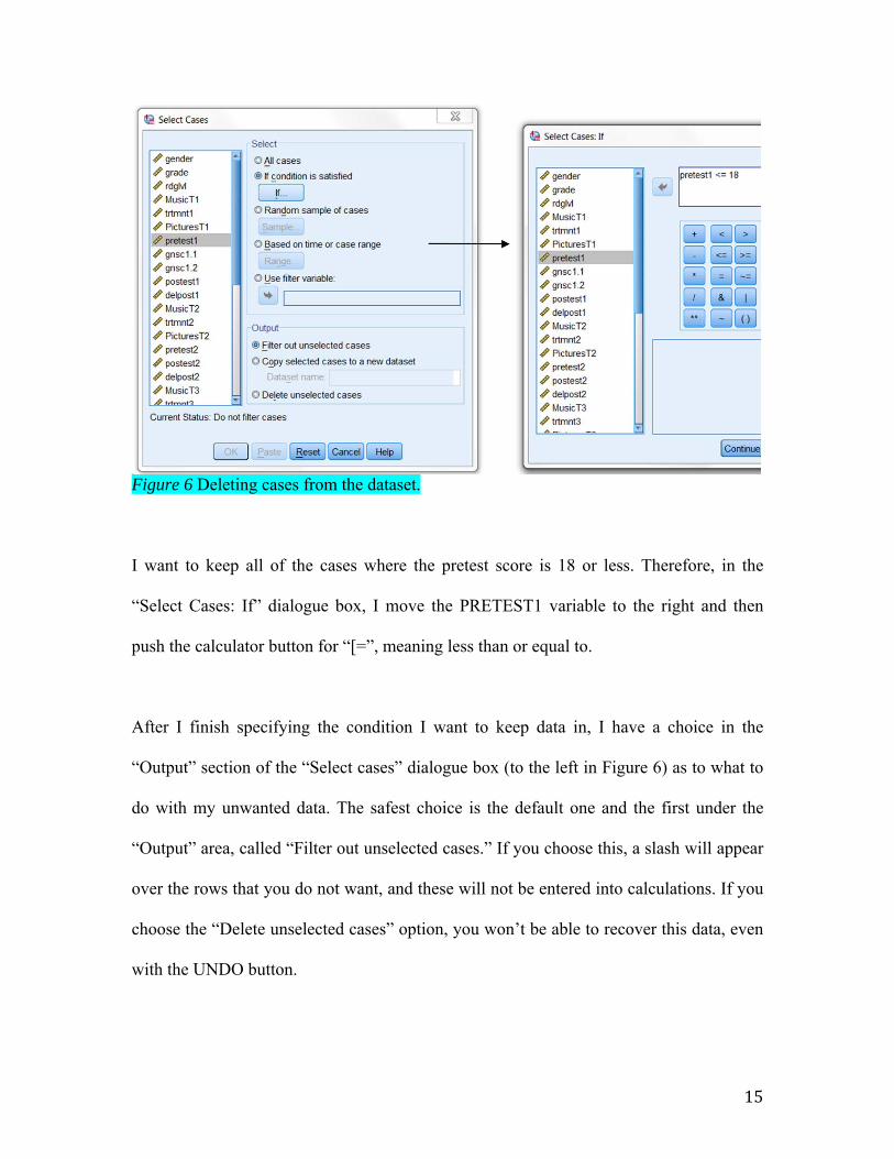
Figure 6 Deleting cases from the dataset.

I want to keep all of the cases where the pretest score is 18 or less. Therefore, in the

“Select Cases: If” dialogue box, I move the PRETEST1 variable to the right and then

push the calculator button for “[=”, meaning less than or equal to.

After I finish specifying the condition I want to keep data in, I have a choice in the

“Output” section of the “Select cases” dialogue box (to the left in Figure 6) as to what to

do with my unwanted data. The safest choice is the default one and the first under the

“Output” area, called “Filter out unselected cases.” If you choose this, a slash will appear

over the rows that you do not want, and these will not be entered into calculations. If you

choose the “Delete unselected cases” option, you won’t be able to recover this data, even

with the UNDO button.

16

 Application Activity for Selecting Cases  

1 Open the DeKeyser2000.sav file. Select only the participants under 15 (Group 1).

2 Open LarsonHall.Forgotten.sav. Pretend I want to exclude all participants who

have spent more than four weeks overseas. How many participants are excluded?

Sorting Variables   You might like to order the data in a column from smallest to largest or vice versa. To do

this, choose the menu options DATA > SORT CASES. The rows of the entire file will be

reordered in order to show a sorting order in the column you choose. You can choose to

sort by just one variable or by several. If you sort by several variables, the one you insert

first will take priority. If there are then ties, the second variable will decide the order.

Figure 7 shows the results of sorting the column PRETEST1 from the Obarow dataset. In

SPSS version 22 this works just as you would expect it to. In earlier versions (version

16), the column would lose its name and also be moved to the beginning of the

spreadsheet. Notice that by ordering it is easy to see that two cases are missing data. Also

notice that the numbers that define the rows stayed the same, even though the data was

moved around. Do not depend on the SPSS row numbers to define your participants—put

in your own column with some kind of ID number for your participants. If you do this,

that ID number will move with each case (row) when the data file is sorted and you will

be able to remember which row of data belongs to which participant!

17

Figure 7 Sorting a column in ascending order (from smallest to largest value).  Application Activities for Manipulating Variables   In this section you will bring together many of the skills you learned about for

manipulating variables in SPSS to accomplish these tasks:

1 Add a new column to the DeKeyser2000.sav file entitled AGEGROUP. Split the

participants into groups depending on their age of arrival (AGE) to the US by

decades. So, for example, you will have one group for those who were 10 or

under, another group for those 11–20, and so on. How many groups do you have?

Label your new groups in the “Variable View” tab. Delete the old column

STATUS. Do a simple report to see if your values are appearing: Go to

ANALYZE > DESCRIPTIVE STATISTICS > FREQUENCIES and put the

AGEGROUP column in the box on the right. Press OK. You should see a report

that has your new variable names. Save your new SPSS file with the four columns

under the name DeKeyserAltered.

18

2 Open the LarsonHall.Forgotten.sav file. The data come from an unpublished

study on Japanese learners of English who lived in the US as either children or

adults. Move the RLWTEST variable from the end of the file to be the first

variable after ID. This variable is a variable with 96 points. Reduce it to two

groups by dividing at the halfway point to separate those who are better and worse

at distinguishing R/L/W in English, or, if you have read the Advanced Topic

section on using Visual Binning, do that to find a suitable cutpoint. Save the file

as LarsonHallAltered.

3 Open the LarsonHallAltered.sav file (you should have created it in step 2). Create

a new variable, TALKTIME, with four categories that distinguish between

participants’ use of English (you’ll use the ENGUSE variable and reduce it to

four groups). Create the groups so that ENGUSE has the following cuts: lowest-8,

9–11, 12–13, 14–highest. Prepare the file so that only participants with data in the

RETURNAGE column will be evaluated. Sort the file by ascending order of

AGE. How many participants were 18 when tested?

4 Open the BEQ.Swear.sav file. The data come from a very large-scale study on

bilinguals conducted by Jean-Marc Dewaele and Aneta Pavlenko (2001–2003).

The column AGESEC refers to the age of acquisition of a second language. First,

move the column so it is the first column in the Data Editor. Filter out any

participants who learned their second language at age zero. Count how many

participants are left by going to ANALYZE > DESCRIPTIVE STATISTICS >

DESCRIPTIVES. Move the AGESEC variable to the right and press OK.

19

5 Open the BeautifulRose.sav file. For the adjective test, not all of the participants

answered the questions in the way the researcher wanted, so the total possible

number of adjectives varies by participant. Let’s say the researcher wanted to

change these scores into percentages so the scores of all participants are

comparable. Calculate a new variable called ADJPERCENT that gives the

percentage correct of each participant. What is the highest percentage correct?

 Bibliography  DeKeyser, R. M. (2000). The robustness of critical period effects in second language

acquisition. Studies in Second Language Acquisition, 22, 499–533.

Dewaele, J.-M., & Pavlenko, A. (2001–2003). Webquestionnaire: Bilingualism and

Emotions. University of London, London.

Larson-Hall, J. & Herrington, R. (2009). Improving data analysis in second language

acquisition by utilizing modern developments in applied statistics. Applied

Linguistics, 31(3), 368–390.

Torres, J. (2004). Speaking up! Adult ESL students’ perceptions of native and non-native

English speaking teachers. Unpublished MA, University of North Texas, Denton.