manova. multivariate (multiple) analysis of variance (manova) represents a blend of univariate...
TRANSCRIPT

MANOVA

• Multivariate (multiple) analysis of variance (MANOVA) represents a blend of univariate analysis of variance principles and canonical correlation analysis.
• It is understood best against the backdrop of basic univariate analysis of variance (ANOVA).
• It is strongly related to discriminant function analysis
• MANOVA & DA are strongly related but conceptually distinct Math is virtually identical -- but direction of prediction or understanding is switched
MANOVA
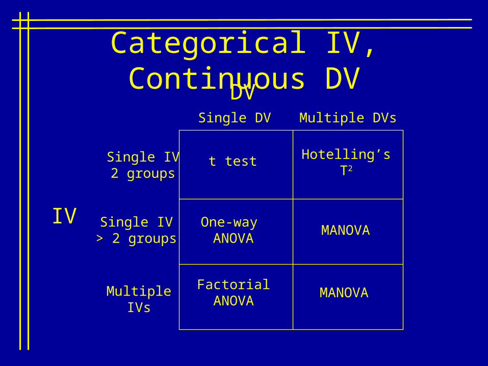
Categorical IV, Continuous DV
IV
Single IV 2 groups
Single IV> 2 groups
MultipleIVs
DVSingle DV Multiple DVs
t test
One-way ANOVA
FactorialANOVA
Hotelling’sT2
MANOVA
MANOVA
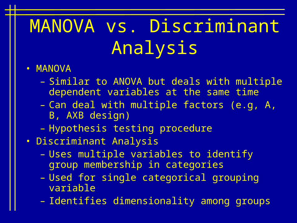
MANOVA vs. Discriminant Analysis
• MANOVA– Similar to ANOVA but deals with multiple dependent
variables at the same time– Can deal with multiple factors (e.g, A, B, AXB design)– Hypothesis testing procedure
• Discriminant Analysis– Uses multiple variables to identify group membership
in categories– Used for single categorical grouping variable– Identifies dimensionality among groups
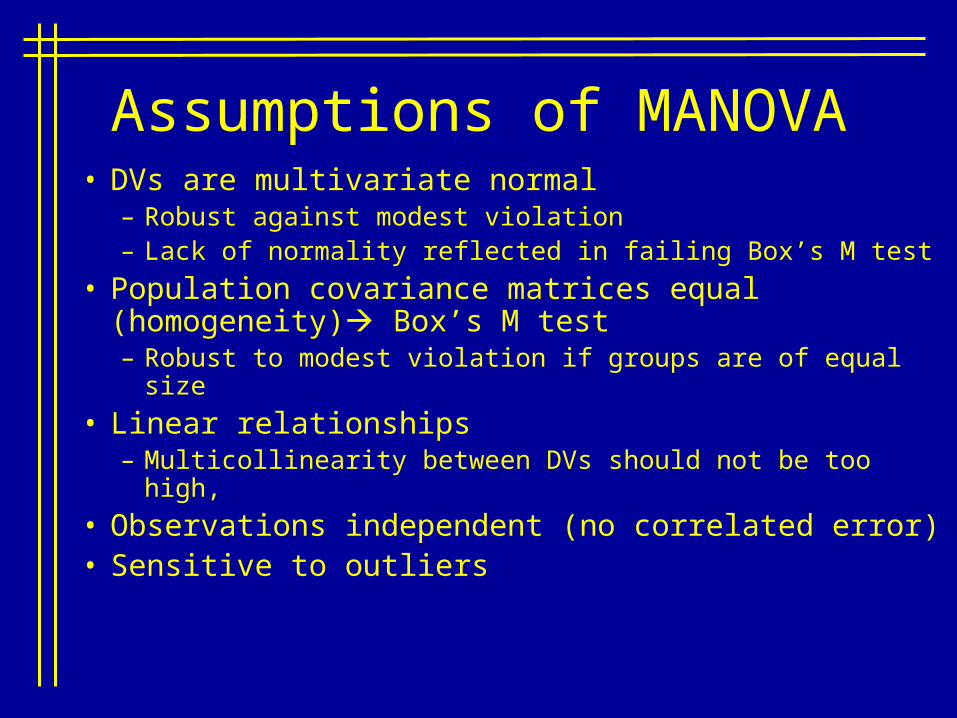
Assumptions of MANOVA• DVs are multivariate normal
– Robust against modest violation– Lack of normality reflected in failing Box’s M test
• Population covariance matrices equal (homogeneity) Box’s M test– Robust to modest violation if groups are of equal size
• Linear relationships– Multicollinearity between DVs should not be too high,
• Observations independent (no correlated error)• Sensitive to outliers
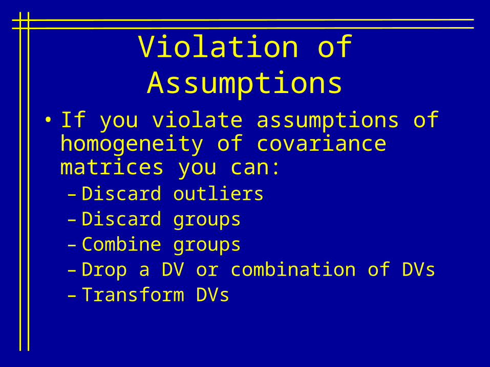
Violation of Assumptions
• If you violate assumptions of homogeneity of covariance matrices you can:– Discard outliers– Discard groups– Combine groups– Drop a DV or combination of DVs– Transform DVs
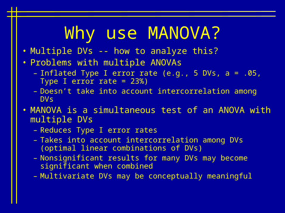
Why use MANOVA?• Multiple DVs -- how to analyze this?• Problems with multiple ANOVAs
– Inflated Type I error rate (e.g., 5 DVs, a = .05, Type I error rate = 23%)
– Doesn’t take into account intercorrelation among DVs
• MANOVA is a simultaneous test of an ANOVA with multiple DVs– Reduces Type I error rates– Takes into account intercorrelation among DVs (optimal linear
combinations of DVs)– Nonsignificant results for many DVs may become significant
when combined– Multivariate DVs may be conceptually meaningful

ANOVA Review
• ANOVAHo: m1 = m2 = ... = mk
Tested by: SSbtwn / SSwithin
SStotal = SSbtwn + SSwithin

MANOVA
Ho
A
B
C
D
A
B
C
D
kA
kB
kC
kD
:
... ...
...
...
1
1
1
1
2
2
2
2
Tested by: MAX B / Werror
T = B + W

MANOVA• Creates linear combinations of DVs that
optimally discriminate among groups– Goal: maximizes discrimination among groups– Each linear combination is orthogonal
• Number of linear combinations extracted for each hypothesis test is equal to df for hypothesis or number of DVs, whichever is smaller (different numbers of linear combinations for different hypothesis tests)

Overall MV Significance Tests• Each MV test provides an approximate F test for
a particular effect on all of the DVs taken together; Tests made of different combinations of matrices, but often yield same result
• Wilks’ Lambda ()– Depends on multiplication of is (differences across
various dimensions)• Pillai’s Trace (V)
– Depends on summation of is (differences across various dimensions)
– Most robust against violations of MV normality and homogeneity of covariance matrices
– More robust when sample size low or unequal cell sizes appear
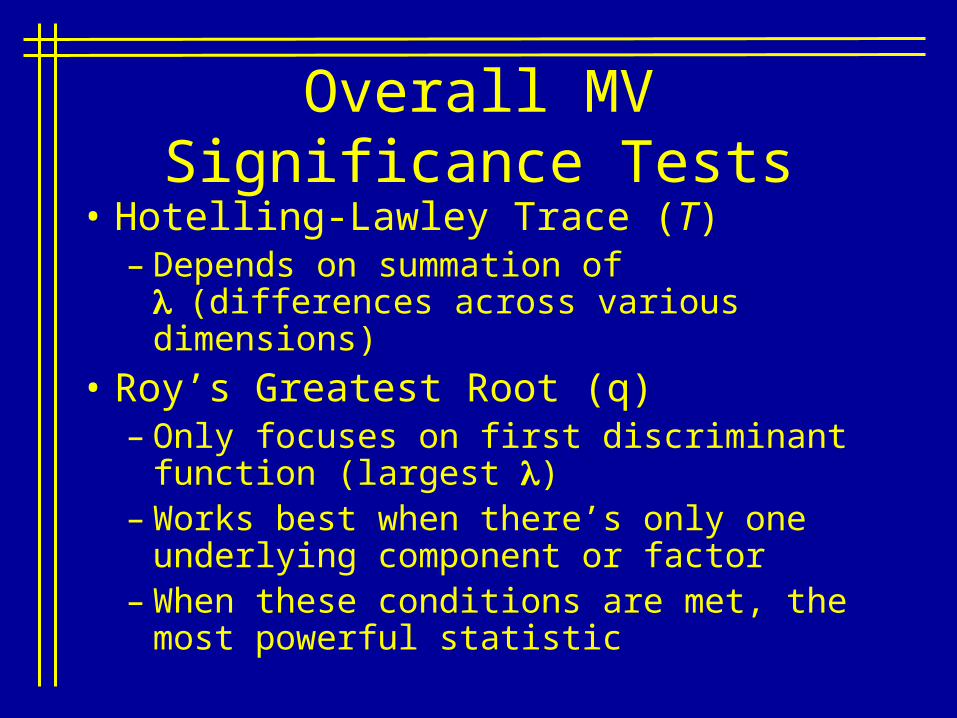
• Hotelling-Lawley Trace (T)– Depends on summation of (differences
across various dimensions)
• Roy’s Greatest Root (q)– Only focuses on first discriminant function
(largest )– Works best when there’s only one
underlying component or factor– When these conditions are met, the most
powerful statistic
Overall MV Significance Tests
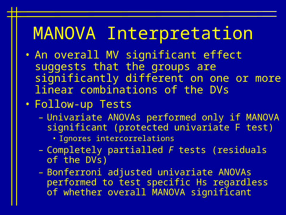
MANOVA Interpretation• An overall MV significant effect suggests that the
groups are significantly different on one or more linear combinations of the DVs
• Follow-up Tests– Univariate ANOVAs performed only if MANOVA
significant (protected univariate F test)• Ignores intercorrelations
– Completely partialled F tests (residuals of the DVs)– Bonferroni adjusted univariate ANOVAs performed to
test specific Hs regardless of whether overall MANOVA significant

MANOVA Interpretation• Can use discriminant weights to interpret
– Like b weights in regression– Susceptible to same problems as b weights
(intercorrelation, cross-validation)
• Can use discriminant loadings to interpret results– AKA structure coefficients or canonical variate
correlations
• Reporting MANOVA– Describe MV test statistic used– Approximate F test and df– Effect size

MANOVA• Assume you have high performing employees that
exhibit different trends of performance (improving, maintaining, declining) that are due to different causes (ability, effort, ease of job)
• You have four DVs– Pay (change in pay)– Promotion (likelihood to promote)– Expect (expected future performance)– Affect (your feelings toward the employee)
• Design is 3 (trend) by 3 (cause) ANOVA with four DVs

Ability Effort Ease of Job
Improving
Maintaining
Declining
MANOVA
Four DVs: (1) Pay (change in pay); (2) Promotion (likelihood to promote); (3) Expect (expected future performance); (4) Affect (your feelings toward the employee)
TREND
CAUSE
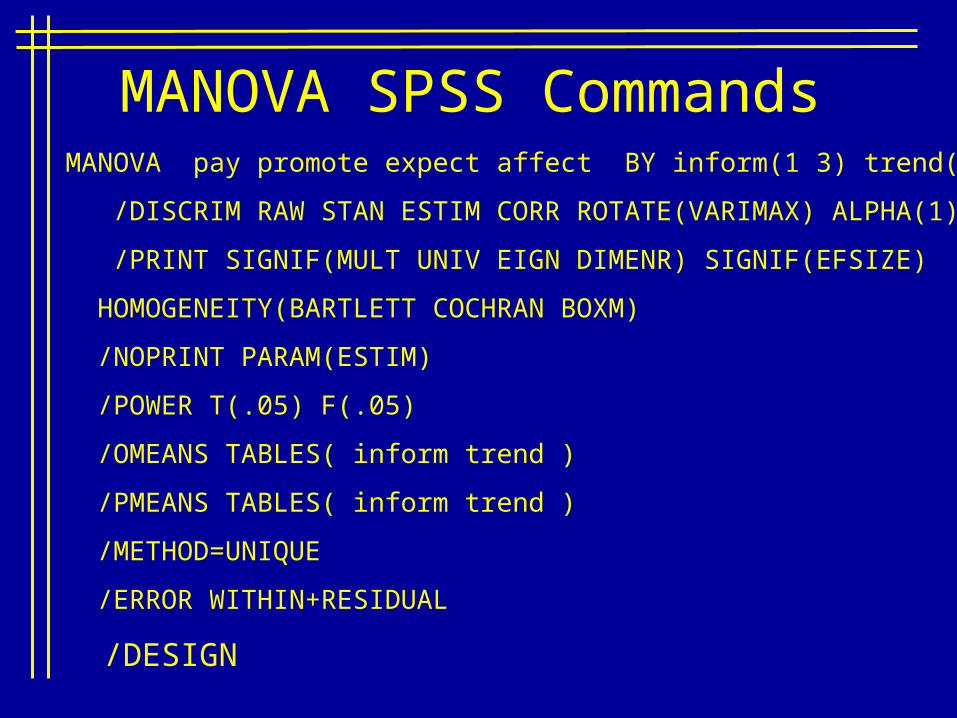
MANOVA pay promote expect affect BY inform(1 3) trend(1 3)
/DISCRIM RAW STAN ESTIM CORR ROTATE(VARIMAX) ALPHA(1)
/PRINT SIGNIF(MULT UNIV EIGN DIMENR) SIGNIF(EFSIZE)
HOMOGENEITY(BARTLETT COCHRAN BOXM)
/NOPRINT PARAM(ESTIM)
/POWER T(.05) F(.05)
/OMEANS TABLES( inform trend )
/PMEANS TABLES( inform trend )
/METHOD=UNIQUE
/ERROR WITHIN+RESIDUAL
/DESIGN
MANOVA SPSS Commands

EFFECT .. TREND
Multivariate Tests of Significance (S = 2, M = 1/2, N = 372 1/2)
Test Name Value Appr. F Hyp. DF Err DF Sig. of F
Pillais .067 6.52 8.00 1496.00 .000
Hotellings .071 6.60 8.00 1492.00 .000
Wilks .933 6.56 8.00 1494.00 .000
Roys .055
Multivariate Effect Size and Observed Power at .0500 Level
TEST NAME Effect Size Noncent. Power
Pillais .034 52.175 1.00
Hotellings .034 52.765 1.00
Wilks .034 52.470 1.00
Results - Trend

Univariate F-tests with (2,750) D. F.
Variable Hyp. SS Err SS Hyp. MS Err MS F Sig. of F
PAY 24.34 28316.6 12.17 37.76 .322 .725
PROMOTE 40.94 12750.9 20.47 17.00 1.204 .301
EXPECT 270.76 9526.0 135.38 12.70 10.659 .000
AFFECT 79.17 12532.4 39.59 16.71 2.369 .094
EFFECT .. TREND (Cont.)
Univariate F-tests with (2,750) D. F. (Cont.)
Variable ETA Square Noncent. Power
PAY .00086 .64475 .10554
PROMOTE .00320 2.40782 .26224
EXPECT .02764 21.31717 .98943
AFFECT .00628 4.73821 .47909
Results - Trend
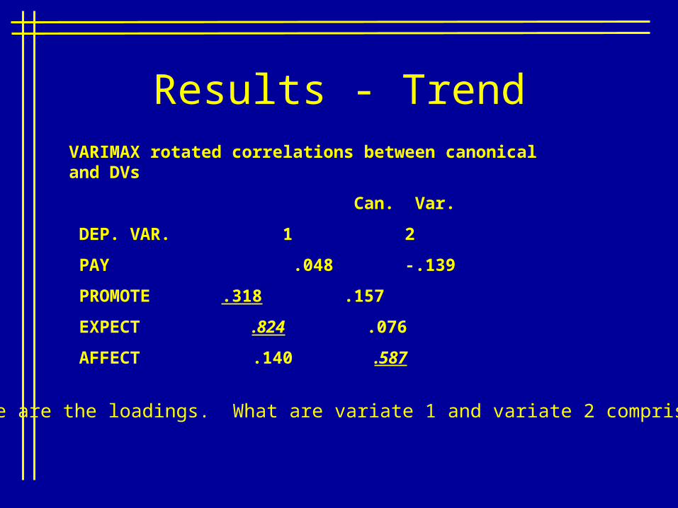
Results - TrendVARIMAX rotated correlations between canonical and DVs
Can. Var.
DEP. VAR. 1 2
PAY .048 -.139
PROMOTE .318 .157
EXPECT .824 .076
AFFECT .140 .587
These are the loadings. What are variate 1 and variate 2 comprised of?

Results
AFFECT
EXPECT
PAY
PROMOTE
TREND
DecliningMaintainingImproving
Me
anZ
Sco
re.2
.1
.0
-.1
-.2
-.3
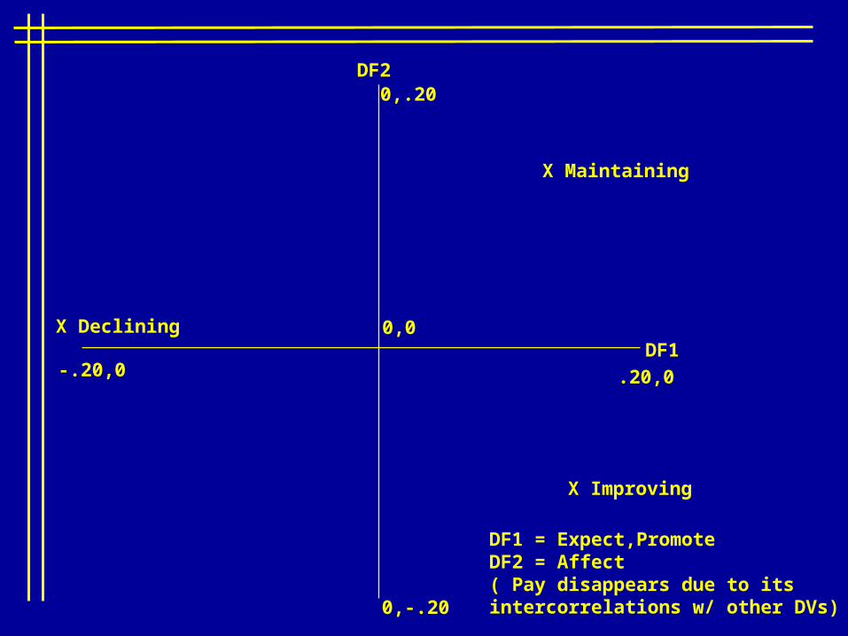
0,0
.20,0-.20,0
0,-.20
0,.20
X Improving
X Maintaining
X Declining
DF2
DF1
DF1 = Expect,PromoteDF2 = Affect( Pay disappears due to its intercorrelations w/ other DVs)
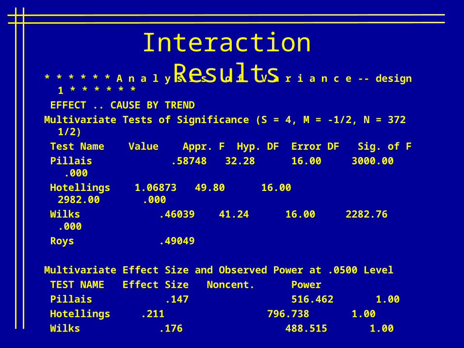
* * * * * * A n a l y s i s o f V a r i a n c e -- design 1 * * * * * *
EFFECT .. CAUSE BY TREND
Multivariate Tests of Significance (S = 4, M = -1/2, N = 372 1/2)
Test Name Value Appr. F Hyp. DF Error DF Sig. of F
Pillais .58748 32.28 16.00 3000.00 .000
Hotellings 1.06873 49.80 16.00 2982.00 .000
Wilks .46039 41.24 16.00 2282.76 .000
Roys .49049
Multivariate Effect Size and Observed Power at .0500 Level
TEST NAME Effect Size Noncent. Power
Pillais .147 516.462 1.00
Hotellings .211 796.738 1.00
Wilks .176 488.515 1.00
Interaction Results

EFFECT .. INFORM BY TREND (Cont.)
Univariate F-tests with (4,750) D. F.
Variable Hyp. SS Err SS Hyp. MS Err MS F Sig. of F
PAY 15569.8 28316.6 3892.4 37.76 103.10 .000
PROMOT 8819.4 12750.9 2204.9 17.00 129.69 .000
EXPECT 3400.2 9526.0 850.0 12.70 66.93 .000
AFFECT 9053.6 12532.4 2263.4 16.71 135.45 .000
EFFECT .. INFORM BY TREND (Cont.)
Univariate F-tests with (4,750) D. F. (Cont.)
Variable ETA Square Noncent. Power
PAY .355 412.39 1.00000
PROMOTE .409 518.75 1.00000
EXPECT .263 267.70 1.00000
AFFECT .419 541.82 1.00000
Interaction Results
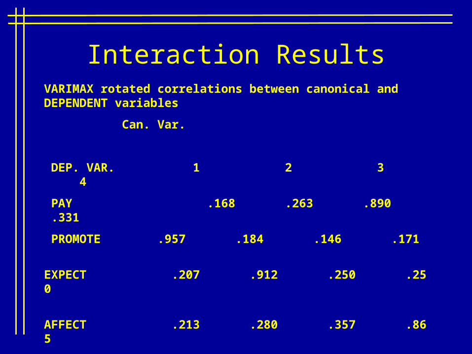
Interaction ResultsVARIMAX rotated correlations between canonical and DEPENDENT variables
Can. Var.
DEP. VAR. 1 2 3 4
PAY .168 .263 .890 .331
PROMOTE .957 .184 .146 .171
EXPECT .207 .912 .250 .250
AFFECT .213 .280 .357 .865
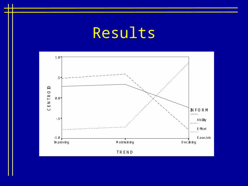
INFORM
Ability
Effort
EaseJob
CE
NT
RO
ID
1.0
.5
0.0
-.5
-1.0
TREND
DecliningMaintainingImproving
Results
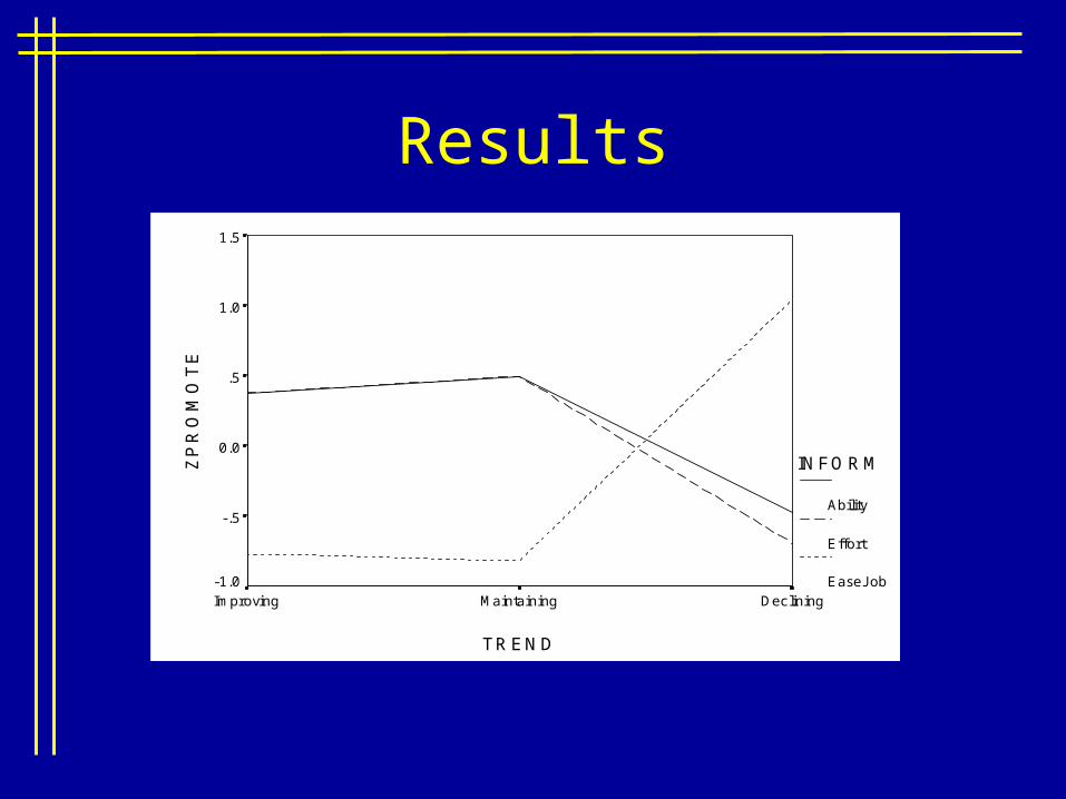
INFORM
Ability
Effort
EaseJob
ZP
RO
MO
TE
1.5
1.0
.5
0.0
-.5
-1.0
TREND
DecliningMaintainingImproving
Results

MANOVA Problems• No guarantee that the linear combinations of DVs will make sense
– Rotation of discriminant function can help• Significance tests on each of DVs can yield conflicting results
when compared to the overall MV significance test• Capitalization on chance
– Cross-validation is crucial• Intercorrelation creates problems with discriminant weights and
their interpretation• Washing out effect (including many nonsig DVs with only a few
signif DVs)• Low power
– Power generally declines as number of DVs increases

One hundred students, preparing to take the Graduate Record Exam, were randomly assigned to one of four training conditions:
Group 1: No special training
Group 2: Standard “book and paper” training
Group 3: Computer-based training
Group 4: Standard and computer-based training
Example

At the end of the study, all students complete a paper-and-pencil version of the Verbal and Quantitative scales of the GRE. All students also completed computer-administered parallel forms of the paper-and-pencil versions. The order of administration of the four outcome measures was counterbalanced.
Example Cont’d…
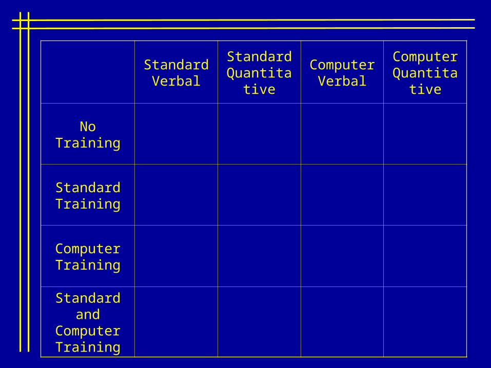
Standard Verbal
Standard Quantitative
Computer Verbal
Computer Quantitative
No Training
Standard Training
Computer Training
Standard and Computer Training

Univariate Analyses
Each Variable Examined Separately
SYNTAXmanova stand_v, stand_q, comp_v, comp_q by group(1,4)/print = cellinfo(all) parameters signif(singledf) homogeneity error/power= exact/design .

Cell Means and Standard Deviations Variable .. STAND_V Standard Measure of Verbal Ability FACTOR CODE Mean Std. Dev. N
GROUP No Train 47.855 10.588 25 GROUP Standard 61.863 12.841 25 GROUP Computer 24.169 11.089 25 GROUP Both 92.450 5.766 25 For entire sample 56.584 26.860 100
- - - - - - - - - - - - - - - - - - - - - - - - - - - - - - - - - - - - - Variable .. STAND_Q Standard Measure of Quantitative Ability FACTOR CODE Mean Std. Dev. N
GROUP No Train 47.517 9.985 25 GROUP Standard 71.831 10.873 25 GROUP Computer 32.781 9.353 25 GROUP Both 81.931 8.764 25 For entire sample 58.515 21.764 100
- - - - - - - - - - - - - - - - - - - - - - - - - - - - - - - - - - - - - Variable .. COMP_V Computer Measure of Verbal Ability FACTOR CODE Mean Std. Dev. N
GROUP No Train 45.720 10.843 25 GROUP Standard 48.774 10.277 25 GROUP Computer 53.363 10.302 25 GROUP Both 82.434 8.784 25 For entire sample 57.573 17.723 100 Variable .. COMP_Q Computer Measure of Quantitative Ability FACTOR CODE Mean Std. Dev. N
GROUP No Train 46.284 10.699 25 GROUP Standard 49.652 10.972 25 GROUP Computer 60.613 9.005 25 GROUP Both 91.507 6.262 25 For entire sample 62.014 20.182 100

GRE Performance as a Function of Training
0
10
20
30
40
50
60
70
80
90
100
No Training Standard Training Computer Training Standard andComputer Training
Training
Pe
rce
nti
le
Standard Verbal GRE
Standard Math GRE
Computer Verbal GRE
Computer Math GRE
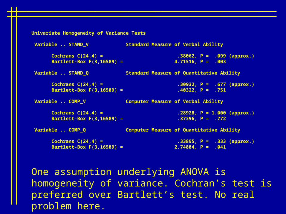
Univariate Homogeneity of Variance Tests
Variable .. STAND_V Standard Measure of Verbal Ability
Cochrans C(24,4) = .38062, P = .099 (approx.) Bartlett-Box F(3,16589) = 4.71516, P = .003
Variable .. STAND_Q Standard Measure of Quantitative Ability
Cochrans C(24,4) = .30932, P = .677 (approx.) Bartlett-Box F(3,16589) = .40322, P = .751
Variable .. COMP_V Computer Measure of Verbal Ability
Cochrans C(24,4) = .28928, P = 1.000 (approx.) Bartlett-Box F(3,16589) = .37396, P = .772
Variable .. COMP_Q Computer Measure of Quantitative Ability
Cochrans C(24,4) = .33895, P = .333 (approx.) Bartlett-Box F(3,16589) = 2.74884, P = .041
One assumption underlying ANOVA is homogeneity of variance. Cochran’s test is preferred over Bartlett’s test. No real problem here.

WITHIN CELLS Correlations with Std. Devs. on Diagonal
STAND_V STAND_Q COMP_V COMP_Q
STAND_V 10.407 STAND_Q .814 9.775 COMP_V .598 .710 10.081 COMP_Q .573 .659 .828 9.423
The multiple outcomes are highly related, especially the different abilities measured by the same method.

EFFECT .. GROUP (Cont.) Univariate F-tests with (3,96) D. F.
Variable Hypoth. SS Error SS Hypoth. MS Error MS F Sig. of F
STAND_V 61029.1914 10396.7654 20343.0638 108.29964 187.84055 .000 STAND_Q 37721.0301 9173.31497 12573.6767 95.55536 131.58525 .000 COMP_V 21342.3217 9755.21167 7114.10723 101.61679 70.00917 .000 COMP_Q 31801.2382 8523.41291 10600.4127 88.78555 119.39344 .000
These omnibus F tests indicate that there are significant group differences for each of the dependent measures. They do not indicate where those differences exist, but there is little doubt that difference do exist.

EFFECT .. 1ST Parameter of GROUP (Cont.) Univariate F-tests with (1,96) D. F.
Variable Hypoth. SS Error SS Hypoth. MS Error MS F Sig. of F
STAND_V 24858.3523 10396.7654 24858.3523 108.29964 229.53310 .000 STAND_Q 14804.6423 9173.31497 14804.6423 95.55536 154.93261 .000 COMP_V 16848.6252 9755.21167 16848.6252 101.61679 165.80553 .000 COMP_Q 25563.6948 8523.41291 25563.6948 88.78555 287.92630 .000
By default, SPSS uses effects coding for the Groups variable, which when unique sums of squares are tested, is a test of each group against the grand mean (except for the last group). The first parameter is thus a test of Group 1 against the grand mean of all groups, for each outcome variable.

EFFECT .. 2ND Parameter of GROUP (Cont.) Univariate F-tests with (1,96) D. F.
Variable Hypoth. SS Error SS Hypoth. MS Error MS F Sig. of F
STAND_V 1145.38103 10396.7654 1145.38103 108.29964 10.57604 .002 STAND_Q 841.89842 9173.31497 841.89842 95.55536 8.81058 .004 COMP_V 3902.96775 9755.21167 3902.96775 101.61679 38.40869 .000 COMP_Q 6172.09410 8523.41291 6172.09410 88.78555 69.51688 .000
The second parameter is a test of Group 2 against the grand mean.

EFFECT .. 3RD Parameter of GROUP (Cont.) Univariate F-tests with (1,96) D. F.
Variable Hypoth. SS Error SS Hypoth. MS Error MS F Sig. of F
STAND_V 35025.4580 10396.7654 35025.4580 108.29964 323.41251 .000 STAND_Q 22074.4893 9173.31497 22074.4893 95.55536 231.01256 .000 COMP_V 590.72871 9755.21167 590.72871 101.61679 5.81330 .018 COMP_Q 65.44923 8523.41291 65.44923 88.78555 .73716 .393
The third parameter is a test of Group 3 against the grand mean. This parameter exhausts the 3 degrees of freedom for the Group effect.

Multivariate Analyses
Variables Treated as Linear Combinations that Maximize Group Separation

Multivariate analysis of variance can be thought of as addressing the question of whether any linear combination among dependent variables can produce a significant separation of groups. In this sense it is similar to canonical correlation analysis in that the linear combination of variables that produces the biggest difference between groups is formed, and if possible, subsequent linear combinations are formed that are independent of the first and that also produce the largest group separation possible.
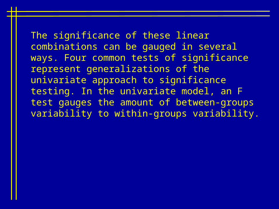
The significance of these linear combinations can be gauged in several ways. Four common tests of significance represent generalizations of the univariate approach to significance testing. In the univariate model, an F test gauges the amount of between-groups variability to within-groups variability.

manova stand_v, stand_q, comp_v, comp_q by group(1,4)/print = cellinfo(means) parameters signif(singledf multiv dimenr eigen univ hypoth) homogeneity error(cor sscp) transform/discrim = stan corr alpha(1)/power= exact/design .
One multivariate approach to these data attempts to find the linear combinations of the four outcome variables that best separate the groups, with no structure imposed on the groups. This would be the most exploratory version.

Pooled within-cells Variance-Covariance matrix
STAND_V STAND_Q COMP_V COMP_Q
STAND_V 108.300 STAND_Q 82.840 95.555 COMP_V 62.760 69.970 101.617 COMP_Q 56.160 60.735 78.667 88.786
Multivariate test for Homogeneity of Dispersion matrices
Boxs M = 100.94212 F WITH (30,25338) DF = 3.10957, P = .000 (Approx.) Chi-Square with 30 DF = 93.40651, P = .000 (Approx.)
This is an assumption underlying MANOVA.

EFFECT .. GROUP Multivariate Tests of Significance (S = 3, M = 0, N = 45 1/2)
Test Name Value Approx. F Hypoth. DF Error DF Sig. of F
Pillais 2.06382 52.35748 12.00 285.00 .000 Hotellings 12.07879 92.26856 12.00 275.00 .000 Wilks .01408 82.31218 12.00 246.35 .000 Roys .86325
As in canonical correlation analysis, this overall test simply indicates whether there are any linear combinations of the outcome variables that can discriminate the groups significantly. It does not indicate how many linear combinations there are.
The rationale for using this omnibus test as a Type I error protection approach is that included among the possible linear combinations are those in which each outcome variable is the only variable receiving a weight.
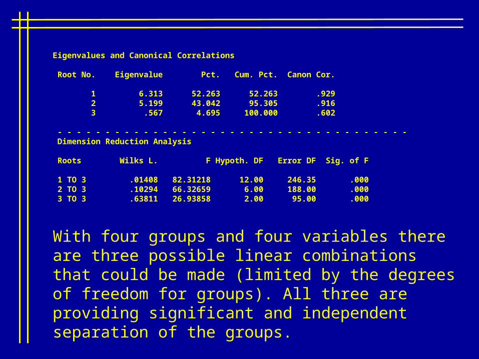
Eigenvalues and Canonical Correlations
Root No. Eigenvalue Pct. Cum. Pct. Canon Cor.
1 6.313 52.263 52.263 .929 2 5.199 43.042 95.305 .916 3 .567 4.695 100.000 .602
- - - - - - - - - - - - - - - - - - - - - - - - - - - - - - - - - - - - - Dimension Reduction Analysis
Roots Wilks L. F Hypoth. DF Error DF Sig. of F
1 TO 3 .01408 82.31218 12.00 246.35 .000 2 TO 3 .10294 66.32659 6.00 188.00 .000 3 TO 3 .63811 26.93858 2.00 95.00 .000
With four groups and four variables there are three possible linear combinations that could be made (limited by the degrees of freedom for groups). All three are providing significant and independent separation of the groups.

EFFECT .. GROUP (Cont.) Standardized discriminant function coefficients Function No.
Variable 1 2 3
STAND_V .804 .713 1.328 STAND_Q .589 -1.219 -1.429 COMP_V -.477 .121 .598 COMP_Q -.188 1.070 -.852
* * * * * * A n a l y s i s o f V a r i a n c e -- design 1 * * * * * *
EFFECT .. GROUP (Cont.) Correlations between DEPENDENT and canonical variables Canonical Variable
Variable 1 2 3
STAND_V .891 .405 .035 STAND_Q .782 .153 -.484 COMP_V .267 .568 -.327 COMP_Q .266 .775 -.538
The canonical variates and loadings are used in the same way here as they were in canonical correlation analysis. What are these linear combinations?
Weights
Loadings
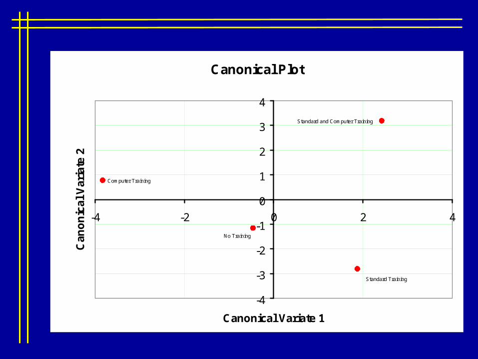
Canonical Plot
Computer Training
Standard and Computer Training
Standard Training
No Training
-4
-3
-2
-1
0
1
2
3
4
-4 -2 0 2 4
Canonical Variate 1
Can
on
ical
Var
iate
2

Canonical Plot
No Training
Standard Training
Standard and Computer Training
Computer Training
-4
-3
-2
-1
0
1
2
3
4
-4 -3 -2 -1 0 1 2 3 4
Canonical Variate 1
Can
on
ical
Var
iate
3

Canonical Plot
Computer Training
Standard and Computer Training
Standard Training
No Training
-4
-3
-2
-1
0
1
2
3
4
-4 -3 -2 -1 0 1 2 3 4
Canonical Variate2
Can
on
ical
Va
riat
e 3

GRE Performance as a Function of Training
-5
-4
-3
-2
-1
0
1
2
3
4
No Training Standard Training Computer Training Standard and ComputerTraining
Training
Can
on
ical
Sco
re
Canonical Variate 1
Canonical Variate 2
Canonical Variate 3

EFFECT .. 1ST Parameter of GROUP Multivariate Tests of Significance (S = 1, M = 1 , N = 45 1/2)
Test Name Value Exact F Hypoth. DF Error DF Sig. of F
Pillais .78886 86.86668 4.00 93.00 .000 Hotellings 3.73620 86.86668 4.00 93.00 .000 Wilks .21114 86.86668 4.00 93.00 .000 Roys .78886 Note.. F statistics are exact.
The default group parameters are effects codes, indicating the extent to which groups are different from the grand mean. This more refined test indicates whether any linear combinations of the outcome variables can discriminate the first group from the grand mean.

Eigenvalues and Canonical Correlations
Root No. Eigenvalue Pct. Cum. Pct. Canon Cor.
1 3.736 100.000 100.000 .888
Because this is inherently the comparison of two “groups”, there is only one way the discrimination can be made.

EFFECT .. 1ST Parameter of GROUP (Cont.) Standardized discriminant function coefficients Function No.
Variable 1
STAND_V -.701 STAND_Q .338 COMP_V .298 COMP_Q -.964
* * * * * * A n a l y s i s o f V a r i a n c e -- design 1 * * * * * *
EFFECT .. 1ST Parameter of GROUP (Cont.) Correlations between DEPENDENT and canonical variables Canonical Variable
Variable 1
STAND_V -.800 STAND_Q -.657 COMP_V -.680 COMP_Q -.896
Just a single linear combination can be formed to make the discrimination.

EFFECT .. 2ND Parameter of GROUP Multivariate Tests of Significance (S = 1, M = 1 , N = 45 1/2)
Test Name Value Exact F Hypoth. DF Error DF Sig. of F
Pillais .74710 68.68199 4.00 93.00 .000 Hotellings 2.95406 68.68199 4.00 93.00 .000 Wilks .25290 68.68199 4.00 93.00 .000 Roys .74710 Note.. F statistics are exact.
A similar test can be made for discriminating the second group from the grand mean.

Eigenvalues and Canonical Correlations
Root No. Eigenvalue Pct. Cum. Pct. Canon Cor.
1 2.954 100.000 100.000 .864
Here too a single linear combination is possible.
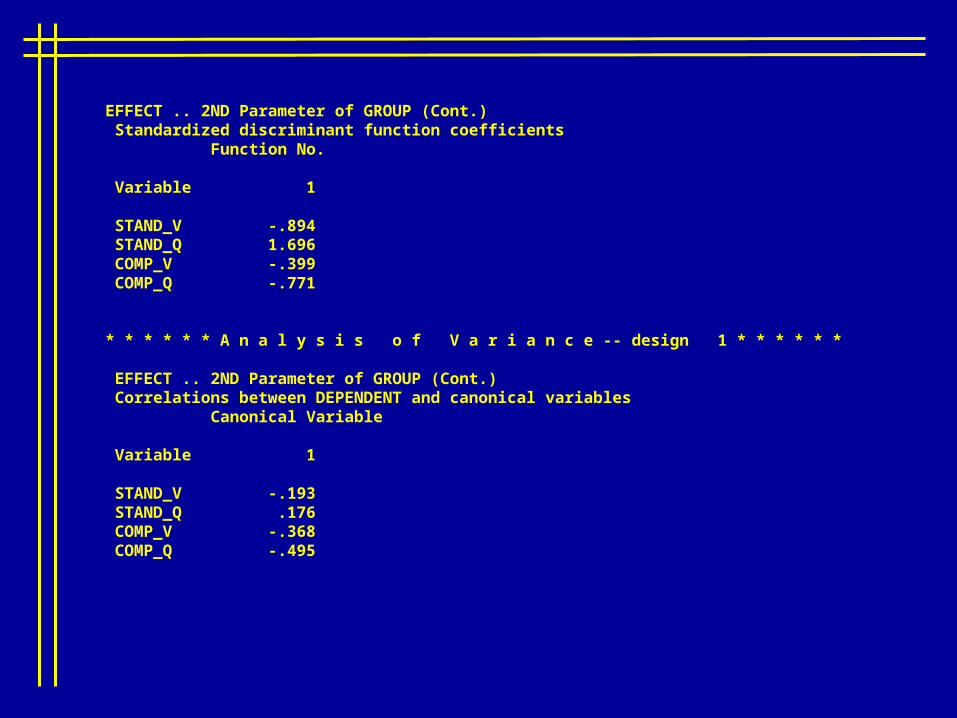
EFFECT .. 2ND Parameter of GROUP (Cont.) Standardized discriminant function coefficients Function No.
Variable 1
STAND_V -.894 STAND_Q 1.696 COMP_V -.399 COMP_Q -.771
* * * * * * A n a l y s i s o f V a r i a n c e -- design 1 * * * * * *
EFFECT .. 2ND Parameter of GROUP (Cont.) Correlations between DEPENDENT and canonical variables Canonical Variable
Variable 1
STAND_V -.193 STAND_Q .176 COMP_V -.368 COMP_Q -.495
EFFECT .. 3RD Parameter of GROUP Multivariate Tests of Significance (S = 1, M = 1 , N = 45 1/2)
Test Name Value Exact F Hypoth. DF Error DF Sig. of F
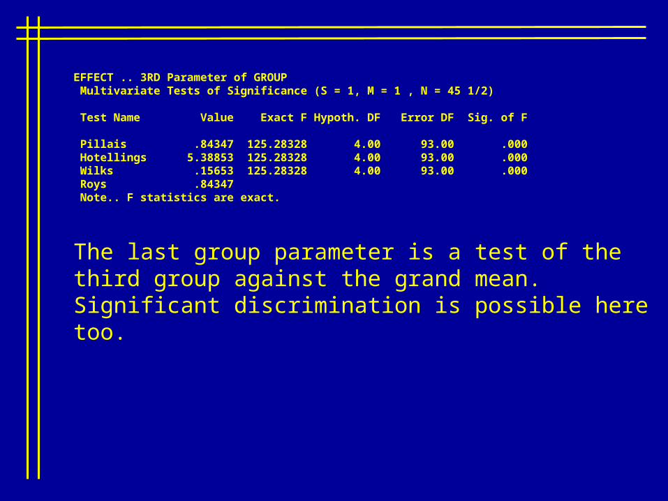
Pillais .84347 125.28328 4.00 93.00 .000 Hotellings 5.38853 125.28328 4.00 93.00 .000 Wilks .15653 125.28328 4.00 93.00 .000 Roys .84347 Note.. F statistics are exact.
The last group parameter is a test of the third group against the grand mean. Significant discrimination is possible here too.
Eigenvalues and Canonical Correlations
Root No. Eigenvalue Pct. Cum. Pct. Canon Cor.
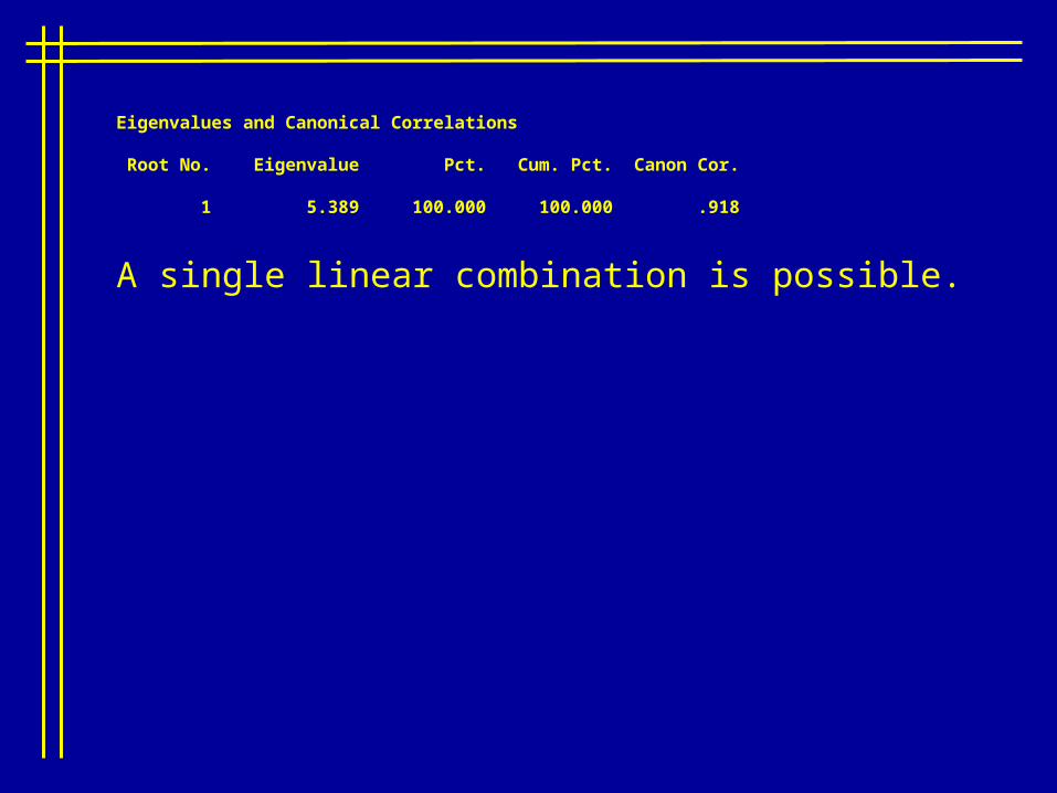
1 5.389 100.000 100.000 .918
A single linear combination is possible.

EFFECT .. 3RD Parameter of GROUP (Cont.) Standardized discriminant function coefficients Function No.
Variable 1
STAND_V .810 STAND_Q .632 COMP_V -.411 COMP_Q -.502
* * * * * * A n a l y s i s o f V a r i a n c e -- design 1 * * * * * *
EFFECT .. 3RD Parameter of GROUP (Cont.) Correlations between DEPENDENT and canonical variables Canonical Variable
Variable 1
STAND_V .791 STAND_Q .668 COMP_V .106 COMP_Q .038
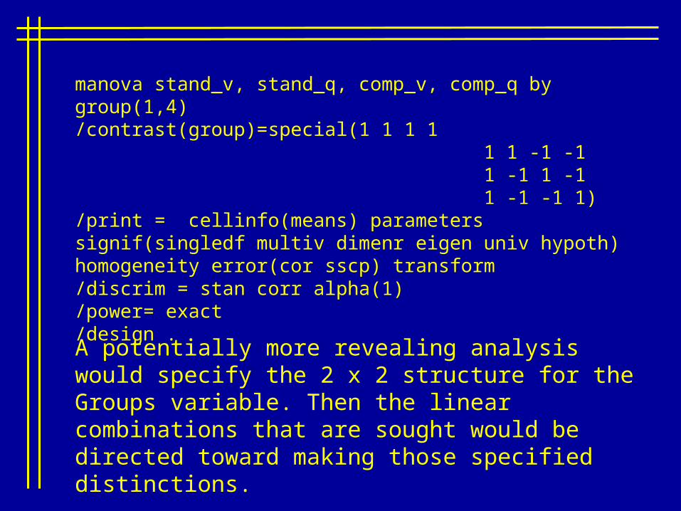
manova stand_v, stand_q, comp_v, comp_q by group(1,4)/contrast(group)=special(1 1 1 1 1 1 -1 -1 1 -1 1 -1 1 -1 -1 1)/print = cellinfo(means) parameters signif(singledf multiv dimenr eigen univ hypoth) homogeneity error(cor sscp) transform/discrim = stan corr alpha(1)/power= exact/design .
A potentially more revealing analysis would specify the 2 x 2 structure for the Groups variable. Then the linear combinations that are sought would be directed toward making those specified distinctions.

EFFECT .. GROUP Multivariate Tests of Significance (S = 3, M = 0, N = 45 1/2)
Test Name Value Approx. F Hypoth. DF Error DF Sig. of F
Pillais 2.06382 52.35748 12.00 285.00 .000 Hotellings 12.07879 92.26856 12.00 275.00 .000 Wilks .01408 82.31218 12.00 246.35 .000 Roys .86325
As with the univariate analyses, the omnibus test for the multivariate analysis does not change. It simply gauges if any discrimination is possible.
Eigenvalues and Canonical Correlations
Root No. Eigenvalue Pct. Cum. Pct. Canon Cor.
1 6.313 52.263 52.263 .929 2 5.199 43.042 95.305 .916 3 .567 4.695 100.000 .602
- - - - - - - - - - - - - - - - - - - - - - - - - - - - - - - - - - - - - Dimension Reduction Analysis
Roots Wilks L. F Hypoth. DF Error DF Sig. of F
1 TO 3 .01408 82.31218 12.00 246.35 .000 2 TO 3 .10294 66.32659 6.00 188.00 .000 3 TO 3 .63811 26.93858 2.00 95.00 .000
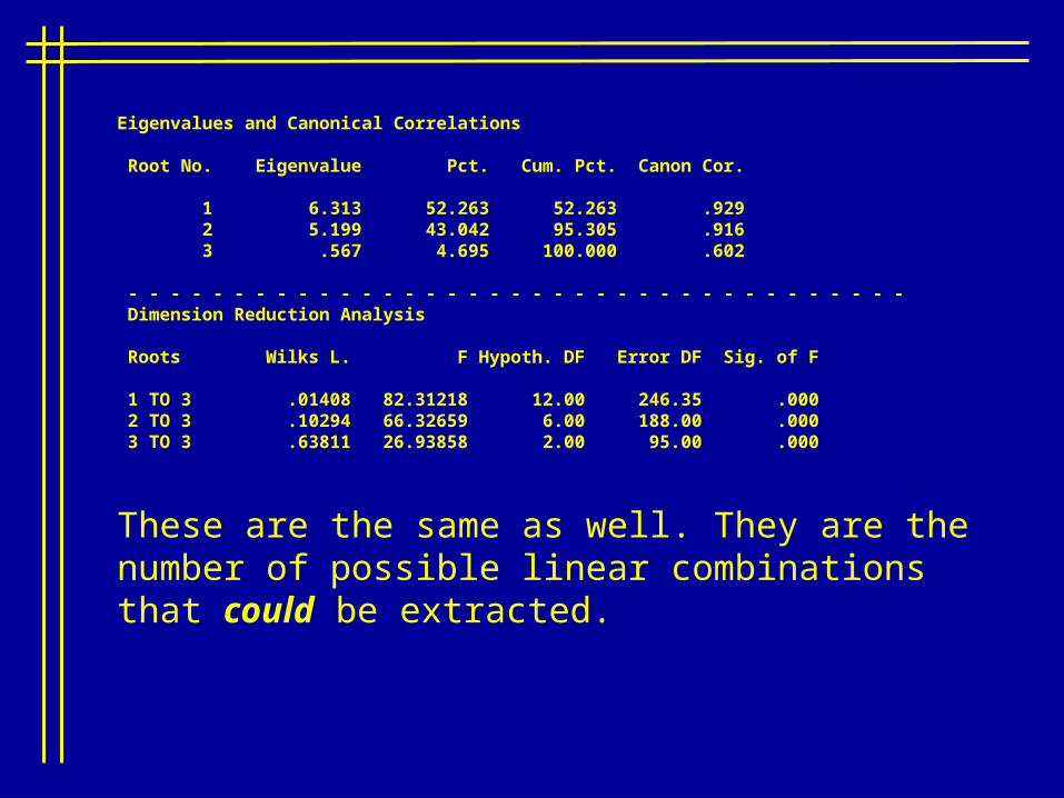
These are the same as well. They are the number of possible linear combinations that could be extracted.

EFFECT .. GROUP (Cont.) Standardized discriminant function coefficients Function No.
Variable 1 2 3
STAND_V .804 .713 1.328 STAND_Q .589 -1.219 -1.429 COMP_V -.477 .121 .598 COMP_Q -.188 1.070 -.852
* * * * * * A n a l y s i s o f V a r i a n c e -- design 1 * * * * * *
EFFECT .. GROUP (Cont.) Correlations between DEPENDENT and canonical variables Canonical Variable
Variable 1 2 3
STAND_V .891 .405 .035 STAND_Q .782 .153 -.484 COMP_V .267 .568 -.327 COMP_Q .266 .775 -.538

EFFECT .. 1ST Parameter of GROUP Multivariate Tests of Significance (S = 1, M = 1 , N = 45 1/2)
Test Name Value Exact F Hypoth. DF Error DF Sig. of F
Pillais .82398 108.83866 4.00 93.00 .000 Hotellings 4.68123 108.83866 4.00 93.00 .000 Wilks .17602 108.83866 4.00 93.00 .000 Roys .82398 Note.. F statistics are exact.
Now the first parameter reflects the structure imposed on the Groups variable. This tests whether it is possible to form a linear combination of the outcome variables that separates the average of the computer-trained groups from the average of the groups that did not receive any computer training.
Eigenvalues and Canonical Correlations
Root No. Eigenvalue Pct. Cum. Pct. Canon Cor.
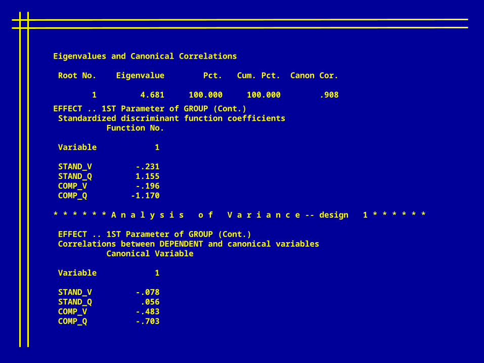
1 4.681 100.000 100.000 .908
EFFECT .. 1ST Parameter of GROUP (Cont.) Standardized discriminant function coefficients Function No.
Variable 1
STAND_V -.231 STAND_Q 1.155 COMP_V -.196 COMP_Q -1.170
* * * * * * A n a l y s i s o f V a r i a n c e -- design 1 * * * * * *
EFFECT .. 1ST Parameter of GROUP (Cont.) Correlations between DEPENDENT and canonical variables Canonical Variable
Variable 1
STAND_V -.078 STAND_Q .056 COMP_V -.483 COMP_Q -.703
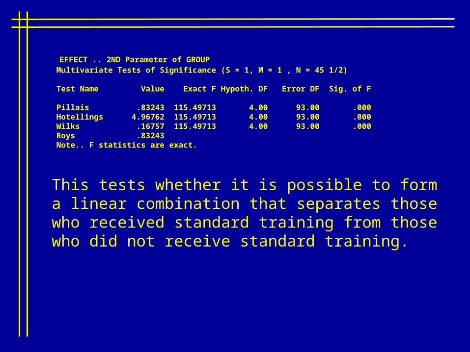
EFFECT .. 2ND Parameter of GROUP Multivariate Tests of Significance (S = 1, M = 1 , N = 45 1/2)
Test Name Value Exact F Hypoth. DF Error DF Sig. of F
Pillais .83243 115.49713 4.00 93.00 .000 Hotellings 4.96762 115.49713 4.00 93.00 .000 Wilks .16757 115.49713 4.00 93.00 .000 Roys .83243 Note.. F statistics are exact.
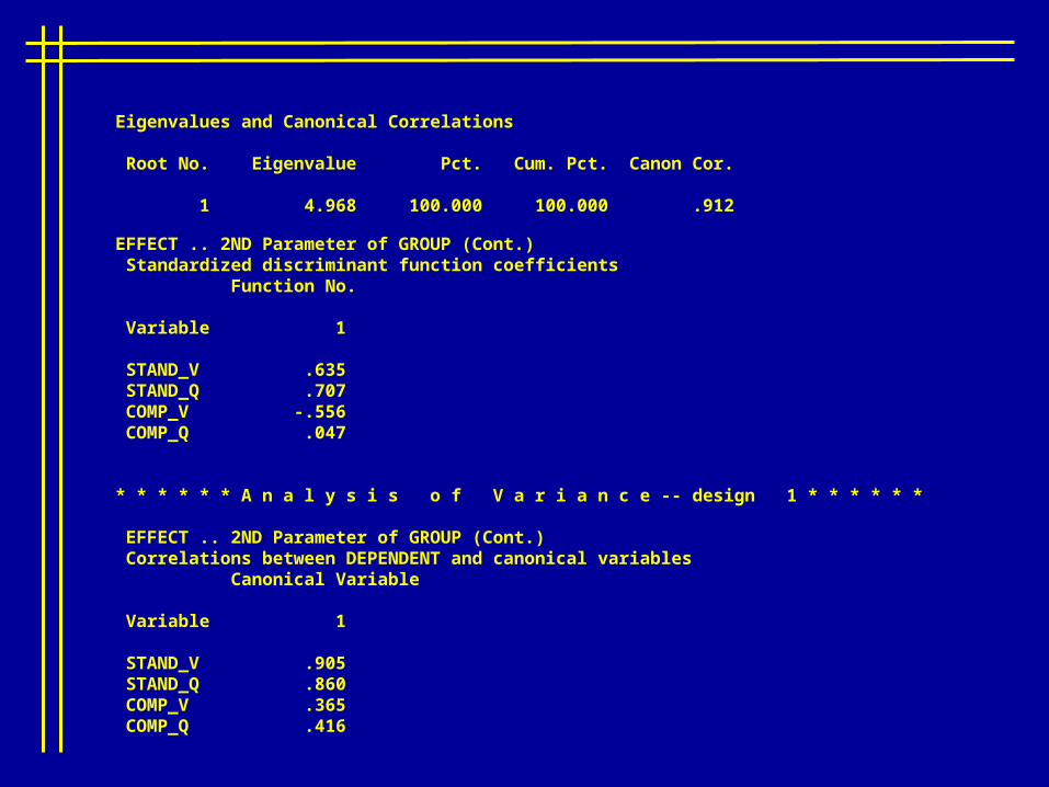
This tests whether it is possible to form a linear combination that separates those who received standard training from those who did not receive standard training.
Eigenvalues and Canonical Correlations
Root No. Eigenvalue Pct. Cum. Pct. Canon Cor.
1 4.968 100.000 100.000 .912
EFFECT .. 2ND Parameter of GROUP (Cont.) Standardized discriminant function coefficients Function No.
Variable 1
STAND_V .635 STAND_Q .707 COMP_V -.556 COMP_Q .047
* * * * * * A n a l y s i s o f V a r i a n c e -- design 1 * * * * * *
EFFECT .. 2ND Parameter of GROUP (Cont.) Correlations between DEPENDENT and canonical variables Canonical Variable
Variable 1
STAND_V .905 STAND_Q .860 COMP_V .365 COMP_Q .416

EFFECT .. 3RD Parameter of GROUP Multivariate Tests of Significance (S = 1, M = 1 , N = 45 1/2)
Test Name Value Exact F Hypoth. DF Error DF Sig. of F
Pillais .70845 56.49617 4.00 93.00 .000 Hotellings 2.42994 56.49617 4.00 93.00 .000 Wilks .29155 56.49617 4.00 93.00 .000 Roys .70845 Note.. F statistics are exact.
The remaining parameter is the interaction. It can be thought of as test of the No Training and Complete Training groups compared to the groups that received just one kind of training.

Eigenvalues and Canonical Correlations
Root No. Eigenvalue Pct. Cum. Pct. Canon Cor.
1 2.430 100.000 100.000 .842
EFFECT .. 3RD Parameter of GROUP (Cont.) Standardized discriminant function coefficients Function No.
Variable 1
STAND_V -1.501 STAND_Q .983 COMP_V -.005 COMP_Q -.263
* * * * * * A n a l y s i s o f V a r i a n c e -- design 1 * * * * * *
EFFECT .. 3RD Parameter of GROUP (Cont.) Correlations between DEPENDENT and canonical variables Canonical Variable
Variable 1
STAND_V -.854 STAND_Q -.416 COMP_V -.422 COMP_Q -.478