manual design pipe systems pumps 608e 1408 tcm11 13269
DESCRIPTION
http://preview.gea.com/global/en/binaries/manual-design-pipe-systems-pumps-608e-1408_tcm11-13269.pdfTRANSCRIPT
Manual for the Design of Pipe Systems and Pumps
engineering for a better world GEA Mechanical Equipment

2
GEA Tuchenhagen
3
GEA Tuchenhagen
1 General
Preface . . . . . . . . . . . . . . . . . . . . . . . . . . . . . . . . . . . . . . . . . . . . . . . . . . . .5
Formula, Units, Designation . . . . . . . . . . . . . . . . . . . . . . . . . . . . . . . . . . .6
2 Introduction
2.1 Pipe systems . . . . . . . . . . . . . . . . . . . . . . . . . . . . . . . . . . . . . . . . . . . . . . . .7
2.2 Liquids . . . . . . . . . . . . . . . . . . . . . . . . . . . . . . . . . . . . . . . . . . . . . . . . . . . . .7
2.3 Centrifugal pump or positive displacement pump . . . . . . . . . . . . . . . . .8
2.4 Tuchenhagen® VARIFLOW Programme . . . . . . . . . . . . . . . . . . . . . . . . . . .8
2.5 Applications . . . . . . . . . . . . . . . . . . . . . . . . . . . . . . . . . . . . . . . . . . . . . . . .9
2.6 Capacity range . . . . . . . . . . . . . . . . . . . . . . . . . . . . . . . . . . . . . . . . . . . . . .9
2.7 Design . . . . . . . . . . . . . . . . . . . . . . . . . . . . . . . . . . . . . . . . . . . . . . . . . . . . .9
2.8 Special features . . . . . . . . . . . . . . . . . . . . . . . . . . . . . . . . . . . . . . . . . . . .10
2.9 Connection fittings . . . . . . . . . . . . . . . . . . . . . . . . . . . . . . . . . . . . . . . . .10
2.10 Accessories and Options . . . . . . . . . . . . . . . . . . . . . . . . . . . . . . . . . . . . .10
2.11 Self-priming centrifugal pumps . . . . . . . . . . . . . . . . . . . . . . . . . . . . . . .11
2.12 Rotary lobe pumps . . . . . . . . . . . . . . . . . . . . . . . . . . . . . . . . . . . . . . . . . .11
3 Physical Fundamentals
3.1 Density . . . . . . . . . . . . . . . . . . . . . . . . . . . . . . . . . . . . . . . . . . . . . . . . . . .12
3.2 Temperature . . . . . . . . . . . . . . . . . . . . . . . . . . . . . . . . . . . . . . . . . . . . . . .12
3.3 Vapour pressure . . . . . . . . . . . . . . . . . . . . . . . . . . . . . . . . . . . . . . . . . . . .12
3.4 Viscosity . . . . . . . . . . . . . . . . . . . . . . . . . . . . . . . . . . . . . . . . . . . . . . . . . .12
3.5 Dynamic viscosity / Kinematice viscosity . . . . . . . . . . . . . . . . . . . . . . . .12
3.6 Fluid behaviour . . . . . . . . . . . . . . . . . . . . . . . . . . . . . . . . . . . . . . . . . . . .13
4 Hydraulic Fundamentals
4.1 Pressure . . . . . . . . . . . . . . . . . . . . . . . . . . . . . . . . . . . . . . . . . . . . . . . . . . .14
4.2 Atmospheric pressure . . . . . . . . . . . . . . . . . . . . . . . . . . . . . . . . . . . . . . .14
4.3 Relation of pressure to elevation . . . . . . . . . . . . . . . . . . . . . . . . . . . . . .14
4.4 Friction losses . . . . . . . . . . . . . . . . . . . . . . . . . . . . . . . . . . . . . . . . . . . . . .15
4.5 Reynolds number . . . . . . . . . . . . . . . . . . . . . . . . . . . . . . . . . . . . . . . . . . .15
5 Technical Fundamentals
5.1 Installation . . . . . . . . . . . . . . . . . . . . . . . . . . . . . . . . . . . . . . . . . . . . . . . .16
5.2 Connection . . . . . . . . . . . . . . . . . . . . . . . . . . . . . . . . . . . . . . . . . . . . . . . .16
5.3 Suction pipe . . . . . . . . . . . . . . . . . . . . . . . . . . . . . . . . . . . . . . . . . . . . . . .17
5.4 Delivery pipe . . . . . . . . . . . . . . . . . . . . . . . . . . . . . . . . . . . . . . . . . . . . . .17
5.5 NPSH . . . . . . . . . . . . . . . . . . . . . . . . . . . . . . . . . . . . . . . . . . . . . . . . . . . .18
5.6 Suction and delivery conditions . . . . . . . . . . . . . . . . . . . . . . . . . . . . . . .18
5.7 Cavitation . . . . . . . . . . . . . . . . . . . . . . . . . . . . . . . . . . . . . . . . . . . . . . . . .19
Table of Contents Page
4
GEA Tuchenhagen
5.8 Q-H characteristic diagram . . . . . . . . . . . . . . . . . . . . . . . . . . . . . . . . . . . .20
5.9 Flow rate . . . . . . . . . . . . . . . . . . . . . . . . . . . . . . . . . . . . . . . . . . . . . . . . . . .21
5.10 Flow head . . . . . . . . . . . . . . . . . . . . . . . . . . . . . . . . . . . . . . . . . . . . . . . . . . .21
5.11 Plant charcteristic curve . . . . . . . . . . . . . . . . . . . . . . . . . . . . . . . . . . . . . . . .21
5.12 Operating point . . . . . . . . . . . . . . . . . . . . . . . . . . . . . . . . . . . . . . . . . . . . . .21
5.13 Pressure drops . . . . . . . . . . . . . . . . . . . . . . . . . . . . . . . . . . . . . . . . . . . . . . .22
5.14 Theoretical calculation example . . . . . . . . . . . . . . . . . . . . . . . . . . . . . . . . .22
6 Design of Centrifugal Pumps
6.1 Practical calculation example . . . . . . . . . . . . . . . . . . . . . . . . . . . . . . . . . . .24
6.1.1 Calculation . . . . . . . . . . . . . . . . . . . . . . . . . . . . . . . . . . . . . . . . . . . . . . . . . .24
6.1.2 Explanations . . . . . . . . . . . . . . . . . . . . . . . . . . . . . . . . . . . . . . . . . . . . . . . . .25
6.1.3 Calculation of the NPSH . . . . . . . . . . . . . . . . . . . . . . . . . . . . . . . . . . . . . . .25
6.2 Characteristic curve interpretation . . . . . . . . . . . . . . . . . . . . . . . . . . . . . . .26
6.3 Modification . . . . . . . . . . . . . . . . . . . . . . . . . . . . . . . . . . . . . . . . . . . . . . . . .28
6.3.1 Throttling . . . . . . . . . . . . . . . . . . . . . . . . . . . . . . . . . . . . . . . . . . . . . . . . . . .28
6.3.2 Changing the speed . . . . . . . . . . . . . . . . . . . . . . . . . . . . . . . . . . . . . . . . . . .28
6.3.3 Reducing the impeller size . . . . . . . . . . . . . . . . . . . . . . . . . . . . . . . . . . . . .29
6.3.4 Operation in parallel . . . . . . . . . . . . . . . . . . . . . . . . . . . . . . . . . . . . . . . . . .29
6.3.5 Operation in series . . . . . . . . . . . . . . . . . . . . . . . . . . . . . . . . . . . . . . . . . . . .29
6.4 Pumping of viscous media . . . . . . . . . . . . . . . . . . . . . . . . . . . . . . . . . . . . .30
6.4.1 Correction for high viscosities . . . . . . . . . . . . . . . . . . . . . . . . . . . . . . . . . .30
6.4.2 Calculation of the correction factors . . . . . . . . . . . . . . . . . . . . . . . . . . . . .31
7 Design of Rotary Lobe Pumps
7.1 Fundamentals . . . . . . . . . . . . . . . . . . . . . . . . . . . . . . . . . . . . . . . . . . . . . . . .32
7.2 Pump rating conditions . . . . . . . . . . . . . . . . . . . . . . . . . . . . . . . . . . . . . . . .32
7.3 Example . . . . . . . . . . . . . . . . . . . . . . . . . . . . . . . . . . . . . . . . . . . . . . . . . . . .33
7.4 Rating the pump . . . . . . . . . . . . . . . . . . . . . . . . . . . . . . . . . . . . . . . . . . . . .34
7.5 Result . . . . . . . . . . . . . . . . . . . . . . . . . . . . . . . . . . . . . . . . . . . . . . . . . . . . . .35
8 Annex
8.1 Diagram for the calculation of pressure drops . . . . . . . . . . . . . . . . . . . . .36
8.2 Pressure drops of fittings in metre equivalent pipe length . . . . . . . . . . .37
8.3 Pressure drops of valves in metre equivalent pipe length . . . . . . . . . . . .37
8.4 Vapour pressure table for water . . . . . . . . . . . . . . . . . . . . . . . . . . . . . . . .39
8.5 Pressure drops depending on viscosity . . . . . . . . . . . . . . . . . . . . . . . . . . . .40
8.6 SI - Units . . . . . . . . . . . . . . . . . . . . . . . . . . . . . . . . . . . . . . . . . . . . . . . . . . . .45
8.7 Conversion table of foreign units . . . . . . . . . . . . . . . . . . . . . . . . . . . . . . . .46
8.8 Viscosity table . . . . . . . . . . . . . . . . . . . . . . . . . . . . . . . . . . . . . . . . . . . . . . . .47
8.9 Mechanical seals . . . . . . . . . . . . . . . . . . . . . . . . . . . . . . . . . . . . . . . . . . . . .49
8.10 Pump data sheet . . . . . . . . . . . . . . . . . . . . . . . . . . . . . . . . . . . . . . . . . . . . .51
8.11 Assembly instructions . . . . . . . . . . . . . . . . . . . . . . . . . . . . . . . . . . . . . . . . .52
Page
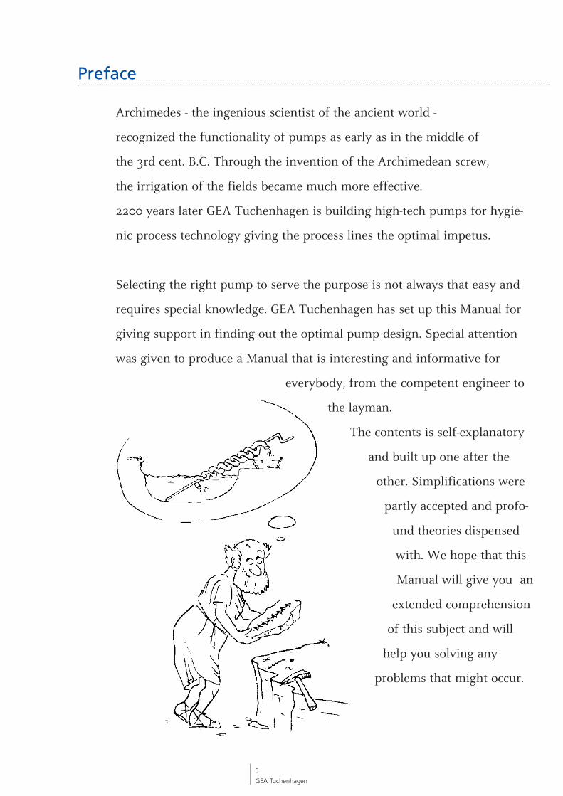
Archimedes - the ingenious scientist of the ancient world -
recognized the functionality of pumps as early as in the middle of
the 3rd cent. B.C. Through the invention of the Archimedean screw,
the irrigation of the fields became much more effective.
2200 years later GEA Tuchenhagen is building high-tech pumps for hygie-
nic process technology giving the process lines the optimal impetus.
Selecting the right pump to serve the purpose is not always that easy and
requires special knowledge. GEA Tuchenhagen has set up this Manual for
giving support in finding out the optimal pump design. Special attention
was given to produce a Manual that is interesting and informative for
everybody, from the competent engineer to
the layman.
The contents is self-explanatory
and built up one after the
other. Simplifications were
partly accepted and profo-
und theories dispensed
with. We hope that this
Manual will give you an
extended comprehension
of this subject and will
help you solving any
problems that might occur.
5
GEA Tuchenhagen
Preface
6
GEA Tuchenhagen
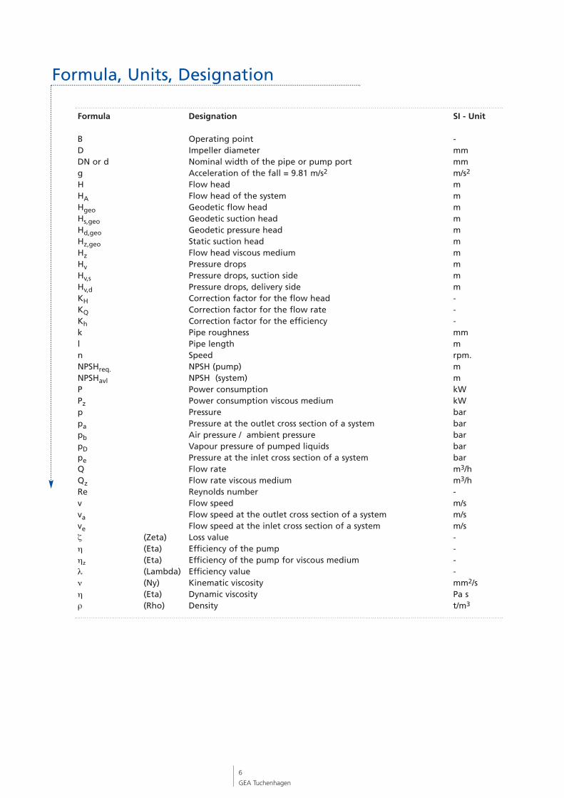
Formula, Units, Designation
Formula Designation SI - Unit
B Operating point -D Impeller diameter mmDN or d Nominal width of the pipe or pump port mmg Acceleration of the fall = 9.81 m/s2 m/s2
H Flow head m HA Flow head of the system m Hgeo Geodetic flow head m Hs,geo Geodetic suction head m Hd,geo Geodetic pressure head m Hz,geo Static suction head m Hz Flow head viscous medium m Hv Pressure drops m Hv,s Pressure drops, suction side m Hv,d Pressure drops, delivery side m KH Correction factor for the flow head -KQ Correction factor for the flow rate -Kh Correction factor for the efficiency -k Pipe roughness mml Pipe length mn Speed rpm. NPSHreq. NPSH (pump) mNPSHavl NPSH (system) mP Power consumption kWPz Power consumption viscous medium kWp Pressure barpa Pressure at the outlet cross section of a system barpb Air pressure / ambient pressure barpD Vapour pressure of pumped liquids barpe Pressure at the inlet cross section of a system barQ Flow rate m3/hQz Flow rate viscous medium m3/hRe Reynolds number -v Flow speed m/sva Flow speed at the outlet cross section of a system m/sve Flow speed at the inlet cross section of a system m/sζ (Zeta) Loss value -η (Eta) Efficiency of the pump -ηz (Eta) Efficiency of the pump for viscous medium -λ (Lambda) Efficiency value -ν (Ny) Kinematic viscosity mm2/sη (Eta) Dynamic viscosity Pa sρ (Rho) Density t/m3
7
GEA Tuchenhagen
The requirements made on process plants steadily increase, both regarding the quality of the products and the profitability of the processes. Making liquids flow solelydue to the earth’s gravitational force is today unthinkable. Liquids are forced throughpipes, valves, heat exchangers, filters and other components, and all of them cause anincreased resistance of flow and thus pressure drops.
Pumps are therefore installed in different sections of a plant. The choice of the right pump atthe right place is crucial and will be responsible for the success or failure of the process. The following factors should be taken into consideration:
1. Installation of the pump
2. Suction and delivery pipes
3. The pump type chosen must correspond to product viscosity, product density, temperature, system pressure, material of the pump, shearing tendency of the product etc.
4. The pump size must conform to the flow rate, pressure, speed, suction conditons etc.
As a manufacturer and supplier of centrifugal pumps and positive displacement pumps weoffer the optimum for both applications. Generally spoken, the pump is a device that conveys a certain volume of a specific liquidfrom point A to point B within a unit of time. For optimal pumping, it is essential before selecting the pump to have examined the pipesystem very carefully as well as the liquid to be conveyed.
Pipe systems have always special characterstics and must be closely inspected for the choiceof the appropriate pump. Details as to considerations of pipe systems are given in Chapter 6,"Design of pumps".
Each liquid possesses diverse characteristics that may influence not only the choice of thepump, but also its configuration such as the type of the mechanical seal or the motor.Fundamental characteristics in this respect are:
• Viscosity (friction losses)• Corrodibility (corrosion)• Abrasion• Temperature (cavitation) • Density • Chemical reaction (gasket material)
2 Introduction
2.1 Pipesystems
2.2 Liquids
Besides these fundamental criteria, some liquids need special care during the transport. The main reasons are:
• The product is sensitive to shearing and could get damaged, such as yoghurt or yoghurtwith fruit pulp
• The liquid must be processed under highest hygienic conditions as practised in the pharmaceutical industry or food industry
• The product is very expensive or toxic and requires hermetically closed transport paths asused in the chemical or pharmaceutical industry.
Experience of many years in research and development of pumps enables GEA Tuchenhagen today to offer a wide range of hygienic pumps for the food and beverage industry as well as the pharmaceutical and chemical industry.
We offer efficient, operationally safe, low-noise pumps for your processes and this Manualshall help you to make the right choice.
The first step on the way to the optimal pump is the selection between a centrifugal pump ora positive displacement pump. The difference lies on one hand in the prin-ciple of transpor-ting the liquid and on the other hand in the pumping characteristic. There are two types ofcentrifugal pumps: "non-self priming" and "selfpriming". Centrifugal pumps are for most of the cases the right choice, because they are easily installed,adapted to different operating parameters and easily cleaned. Competitive purchase costs andreliable transport for most of the liquids are the reason for their steady presence in processplants. Restrictions must be expected in the following cases:
• with viscous media the capacity limit is quickly reached,• the use is also restricted with media being sensitive to shearing,• with abbrasive liquids the service life of the centrifugal pump is reduced
because of earlier wear.
The GEA Tuchenhagen®-VARIFLOW Pump Programme conforms to today’s requirementsmade on cleanability, gentle product handling, efficiency and ease of maintenance.
The different technical innovations made on the pumps for the optimization of cleanability have been EHEDG-certified.
8
GEA Tuchenhagen
2.4 GEA Tuchenhagen®
VARIFLOW Programme
2.3 Centrifugalor positive displacement pump
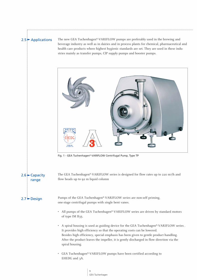
The new GEA Tuchenhagen®-VARIFLOW pumps are preferably used in the brewing andbeverage indus try as well as in dairies and in process plants for chemical, pharmaceu tical andhealth care products where highest hygienic standards are set. They are used in these indu-stries mainly as transfer pumps, ClP supply pumps and booster pumps.
The GEA Tuchenhagen®-VARIFLOW series is designed for flow rates up to 220 m3/h andflow heads up to 92 m liquid column
Pumps of the GEA Tuchenhagen®-VARIFLOW series are non-self priming, one-stage centrifugal pum ps with single bent vanes.
• All pumps of the GEA Tuchenhagen®-VARIFLOW series are driven by standard motors of type IM B35.
• A spiral housing is used as guiding device for the GEA Tuchenhagen®-VARIFLOW series .It provides high efficiency so that the operating costs can be lowered. Besides high efficiency, special emphasis has been given to gentle product handling. After the product leaves the impeller, it is gently discharged in flow direction via the spiral housing.
• GEA Tuchenhagen®-VARIFLOW pumps have been certified according to EHEDG and 3A.
2.6 Capacity range
2.5 Applications
9
GEA Tuchenhagen
Fig. 1 - GEA Tuchenhagen®-VARIFLOW Centrifugal Pump, Type TP
2.7 Design

2.10 Accessories and Options
2.9 Connectionfittings
2.8 Special features
10
GEA Tuchenhagen
• All parts in stainless steel, product wetted components are made of AISI 316L (1.4404).
• High efficiency• Gentle product handling• Low noise• Ease of maintenance• Excellent hygienic properties.
• Threaded joint as per DIN 11851 (Standard)• VARIVENT® flange connection• Aseptic flanges as per DIN 11864-2• Aseptic union as per DIN 11864-1• Other marketable connections according to BS, SMS, RJT, Tri-Clamp• Metric and Inch diameters
• Mechanical seals in different materials Carbon/Silicon carbide or Silicon carbide/Silicon carbide
• Different designs as single acting, single with flush (Quench) or double acting• FDA approved soft seals: EPDM and FPM• Stainless steel protection hood, mobile baseframe, drainage valve• Adjustable calotte type feet frame• Inducer
Fig 2 - GEA Tuchenhagen®-VARIFLOW, TP
Main components:Pump cover, impeller, pump housing lantern, shaft and motor
Impeller
MotorOne-part lantern
Pumpcover
Pump shaftwithout feather key
Mech.shaft seal
Sealing according to the VARIVENT® principle
Pump housing
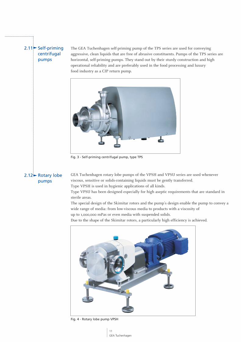
The GEA Tuchenhagen self-priming pump of the TPS series are used for conveying aggressive, clean liquids that are free of abrasive constituents. Pumps of the TPS series arehorizontal, self-priming pumps. They stand out by their sturdy construction and high operational reliability and are preferably used in the food processing and luxury food industry as a CIP return pump.
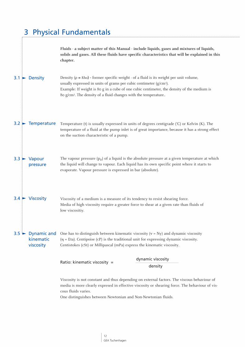
GEA Tuchenhagen rotary lobe pumps of the VPSH and VPSU series are used whenever viscous, sensitive or solids-containing liquids must be gently transferred.Type VPSH is used in hygienic applications of all kinds.Type VPSU has been designed especially for high aseptic requirements that are standard insterile areas. The special design of the Skimitar rotors and the pump’s design enable the pump to convey awide range of media: from low-viscous media to products with a viscosity of up to 1,000,000 mPas or even media with suspended solids. Due to the shape of the Skimitar rotors, a particularly high efficiency is achieved.
2.12 Rotary lobepumps
11
GEA Tuchenhagen
2.11 Self-priming centrifugal pumps
Fig. 4 - Rotary lobe pump VPSH
Fig. 3 - Self-priming centrifugal pump, type TPS
Fluids - a subject matter of this Manual - include liquids, gases and mixtures of liquids,solids and gases. All these fluids have specific characteristics that will be explained in thischapter.
Density (ρ = Rho) - former specific weight - of a fluid is its weight per unit volume, usually expressed in units of grams per cubic centimeter (g/cm3).Example: If weight is 80 g in a cube of one cubic centimeter, the density of the medium is 80 g/cm3. The density of a fluid changes with the temperature..
Temperature (t) is usually expressed in units of degrees centigrade (°C) or Kelvin (K). Thetemperature of a fluid at the pump inlet is of great importance, because it has a strong effecton the suction characteristic of a pump.
The vapour pressure (pD) of a liquid is the absolute pressure at a given temperature at whichthe liquid will change to vapour. Each liquid has its own specific point where it starts to evaporate. Vapour pressure is expressed in bar (absolute).
Viscosity of a medium is a measure of its tendency to resist shearing force. Media of high viscosity require a greater force to shear at a given rate than fluids of low viscositiy.
One has to distinguish between kinematic viscosity (ν = Ny) and dynamic viscosity (η = Eta). Centipoise (cP) is the traditional unit for expressing dynamic viscosity. Centistokes (cSt) or Millipascal (mPa) express the kinematic viscosity.
Ratio: kinematic viscosity =
Viscosity is not constant and thus depending on external factors. The viscous behaviour ofmedia is more clearly expresed in effective viscosity or shearing force. The behaviour of vis-cous fluids varies. One distinguishes between Newtonian and Non-Newtonian fluids.
12
GEA Tuchenhagen
3.5 Dynamic and kinematic viscosity
3.1 Density
3 Physical Fundamentals
3.2 Temperature
3.3 Vapour pressure
3.4 Viscosity
density
dynamic viscosity

The flow curve is a diagram which shows the correlation between viscosity (η) and the shearrate (D). The shear rate is calculated from the ratio between the difference in flow velocity oftwo adjacent fluid layers and their distance to eachother.
The flow curve for an ideal fluid is a straight line. This means constant viscosity at all shearrates. All fluids of this characteristic are "Newtonian fluids". Examples are water, mineral oils,syrup, resins.
Fluids that change their viscosity in dependence of the shear rate are called "Non-Newtonian fluids". In practice, a very high percentage of fluids pumped are non-Newtonian and can be differentiated as follows:
Intrinsically viscous fluidsViscosity decreases as the shear rate increases at high initial force. This means from the technical point of view that the energy after the initial force needed for the flow rate can bereduced. Typical fluids with above described characteristics are a.o. gels, Latex, lotions.Dilatent fluidsViscosity increases as the shear rate increases. Example: pulp, sugar mixtureThixotropic fluidsViscosity decreases with strong shear rate (I) and increases again as the shear rate decreases (II).The ascending curve is however not identical to the descending curve. Typical fluids are a.o.soap, Ketchup, glue, peanut butter
13
GEA Tuchenhagen
3.6 Fluid behaviour
Fig. 6 - Flow curves
Fig. 7 - Thixotropic fluids
Vis
cosi
ty
Shear rate
Vis
cosi
ty
Shear rate
1
2
3 1 Newtonian fluids
2 Intrinsicallyviscous fluids
3 Dilatent fluids
Δy
Δv
Fig. 5 - Shear rate
I
II
D = ΔvΔy
v
4.2 Atmosphericpressure
14
GEA Tuchenhagen
Pumps shall produce pressure. Fluids are conveyed over a certain distance by kinetic ener-gy produced by the pump.
The basic definition of pressure (p) is the force per unit area. It is expressed in this Manual inNewton per square meter (N/m2 = Pa).
1 bar = 105 = 105 Pa
Atmospheric pressure is the force exerted on a unit area by the weight of the atmosphere. Itdepends on the height above sea level (see Fig. 8). At sea level the absolute pressure is approximately 1 bar = 105 N / m2.Gage pressure uses atmospheric pressure as a zero reference and is then measured in relationto atmospheric pressure. Absolute pressure is the atmospheric pressure plus the relative pressure.
In a static liquid the pressure difference between any two points is in direct proportion to thevertical distance between the two points only. The pressure difference is calculated by multiplying the vertical distance by density.In this Manual different pressures or pressure relevant terms are used. Here below are listedthe main terms and their definitions:
Static pressure Hydraulic pressure at a point in a fluid at rest.
Friction loss Loss in pressure or energy due to friction losses in flow
Dynamic pressure Energy in a fluid that occurs due to the flow velocity.
Delivery pressure Sum of static and dynamic pressure increase.
Delivery head Delivery pressure converted into m liquid column.
Differential pressure Pressure between the initial and end point of the plant.
4.1 Pressure
4 Hydraulic Fundamentals
4.3 Relation ofpressure toelevation
Nm2
Height above sea level Air pressure pb Boiling temperaturem bar °C
0 1,013 100200 989 99500 955 98
1,000 899 972,000 795 93
Fig. 8 - Influcence of the topographic height
4.5 Reynolds number
15
GEA Tuchenhagen
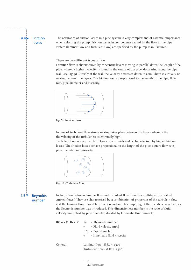
The occurance of friction losses in a pipe system is very complex and of essential importancewhen selecting the pump. Friction losses in components caused by the flow in the pipesystem (laminar flow and turbulent flow) are specified by the pump manufacturer.
There are two different types of flowLaminar flow is characterized by concentric layers moving in parallel down the length of thepipe, whereby highest velocity is found in the centre of the pipe, decreasing along the pipewall (see Fig. 9). Directly at the wall the velocity decreases down to zero. There is virtually nomixing between the layers. The friction loss is proportional to the length of the pipe, flowrate, pipe diameter and viscosity.
In case of turbulent flow strong mixing takes place between the layers whereby the the velocity of the turbulences is extremely high. Turbulent flow occurs mainly in low viscous fluids and is characterised by higher friction losses. The friction losses behave proportional to the length of the pipe, square flow rate, pipe diameter and viscosity.
In transition between laminar flow and turbulent flow there is a multitude of so called„mixed flows“. They are characterised by a combination of properties of the turbulent flowand the laminar flow. For determination and simple computing of the specific characteristicsthe Reynolds number was introduced. This dimensionless number is the ratio of fluid velocity multiplied by pipe diameter, divided by kinematic fluid viscosity.
Re = v x DN / ν Re = Reynolds numberv = Fluid velocity (m/s)DN = Pipe diameterν = Kinematic fluid viscosity
General: Laminar flow - if Re < 2320Turbulent flow - if Re ≥ 2320
4.4 Frictionlosses
Fig. 9 - Laminar flow
Fig. 10 - Turbulent flow
16
GEA Tuchenhagen
This Manual helps carrying out the optimal design of centrifugal pumps. We show youhow to proceed to find the right pump.
Install the pump in close vicinity to the tank or to another source from which the liquid willbe pumped. Make sure that as few as possible valves and bends are integrated in the pump‘ssuction pipe, in order to keep the pressure drop as low as possible. Sufficient space aroundthe pump provides for easy maintenance work and inspection. Pumps equipped with a conventional base plate and motor base should be mounted on a steady foundation and beprecisely aligned prior commissioning.
GEA Tuchenhagen pumps are equipped with pipe connections that are adaped to the flowrate. Very small pipe dimensions result in low cost on one hand, but on the other hand putthe safe, reliable and cavitation-free operation of the pump at risk. Practical experience has shown that identical connection diameters on a short suction pipeare beneficial, however, always keep an eye on the fluid velocity. Excepted thereof are longsuction pipes with integrated valves and bends. In this case the suction pipe should be by onesize larger, in order to reduce the pressure drop.
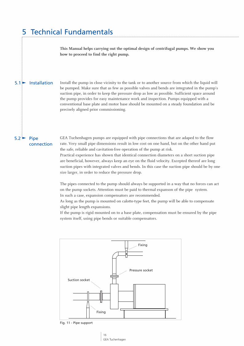
The pipes connected to the pump should always be supported in a way that no forces can acton the pump sockets. Attention must be paid to thermal expanson of the pipe system. In such a case, expansion compensators are recommended. As long as the pump is mounted on calotte-type feet, the pump will be able to compensateslight pipe length expansions. If the pump is rigid mounted on to a base plate, compensation must be ensured by the pipesystem itself, using pipe bends or suitable compensators.
5.1 Installation
5 Technical Fundamentals
5.2 Pipe connection
Fig. 11 - Pipe support
Suction socket
Fixing
Pressure socket
Fixing
17
GEA Tuchenhagen
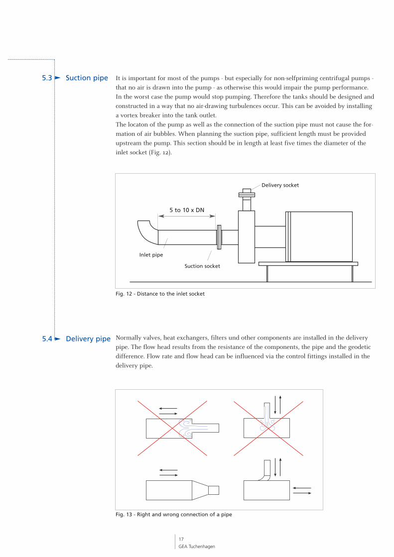
It is important for most of the pumps - but especially for non-selfpriming centrifugal pumps -that no air is drawn into the pump - as otherwise this would impair the pump performance.In the worst case the pump would stop pumping. Therefore the tanks should be designed andconstructed in a way that no air-drawing turbulences occur. This can be avoided by installinga vortex breaker into the tank outlet. The locaton of the pump as well as the connection of the suction pipe must not cause the for-mation of air bubbles. When planning the suction pipe, sufficient length must be providedupstream the pump. This section should be in length at least five times the diameter of theinlet socket (Fig. 12).
Normally valves, heat exchangers, filters und other components are installed in the deliverypipe. The flow head results from the resistance of the components, the pipe and the geodeticdifference. Flow rate and flow head can be influenced via the control fittings installed in thedelivery pipe.
5.3 Suction pipe
5.4 Delivery pipe
Fig. 12 - Distance to the inlet socket
Fig. 13 - Right and wrong connection of a pipe
5 to 10 x DN
Suction socket
Delivery socket
Inlet pipe
5.5 NPSH
18
GEA Tuchenhagen
NPSH (Net Positive Suction Head) is the international dimension for the calculation of thesupply conditions.
For pumps the static pressure in the suction socket must be above the vapour pressure of themedium to be pumped. The NPSH of the pump is determined by measurements carried outon the suction and delivery side of the pump. This value is to be read from the pump charac-teristic curve and is indicated in meter (m). The NPSH is in the end a dimension of the evapo-ration hazard in the pump inlet socket and is influenced by the vapour pressure and the pum-ped liquid. The NPSH of the pump is called NPSH required, and that of the system is calledNPSH av(ai)lable. The NPSHavl should be greater than the NPSHreq in order to avoid cavitation.
NPSHavl > NPSHreq
For safety reasons another 0.5 m should be integrated into the calculation, i.e.:
NPSHavl > NPSHreq + 0.5m
Troublefree operation of centrifugal pumps is given as long as steam cannot form inside thepump; in other words: if cavitation does not occur. Therefore, the pressure at the referencepoint for the NPSH must be at least above the vapour pressure of the pumped liquid. Thereference level for the NPSH is the centre of the impeller so that for calculating the NPSHavl
according to the equation below, the geodetic flow head in the supply mode (Hz,geo) must beset to posi tive and in the suction mode (Hs,geo) to negative
NPSHavl =
pe = Pressure at the inlet cross section of the systempb = Air pressure in N/m2 (consider influence of height)pD = Vapour pressureρ = Density g = Acceleration of the fallve = Flow speedHv,s = Sum of pressure drops Hs,geo = Height difference between liquid level in the suction tank and
centre of the pump suction socket
At a water temperature of 20 °C and with an open tank the formula is simplified:
NPSHavl = 10 - Hv,s + Hz,geo
5.6 Suction andsupply conditions
pe + pb pD ve2
ρ x g ρ x g 2g+- - Hv,s + Hs,geo
5.7 Cavitation
19
GEA Tuchenhagen
Cavitation produces a crackling sound in the pump. Generally spoken is cavitation the forma-tion and collapse of vapour bubbles in the liquid. Cavitation may occur in pipes, valves and inpumps. First the static pressure in the pump falls below the vapour pressure associated to thetemperature of a fluid at the impeller intake vane channel. The reason is in most of the casesa too low static suction head. Vapour bubbles form at the intake vane channel. The pressureincreases in the impeller channel and causes an implosion of the vapour bubbles. The resultis pitting corrosion at the impeller, pressure drops and unsteady running of the pump. Finallycavitation causes damage to the pumped product.
Cavitation can be prevented by :
1. Reducing the pressure drop in the suction pipe by a larger suction pipe diameter, shortersuction pipe length and less valves or bends
2. Increasing the static suction head and/or supply pressure, e.g. by an upstream impeller(Inducer)
3. Lowering the temperature of the pumped liquid
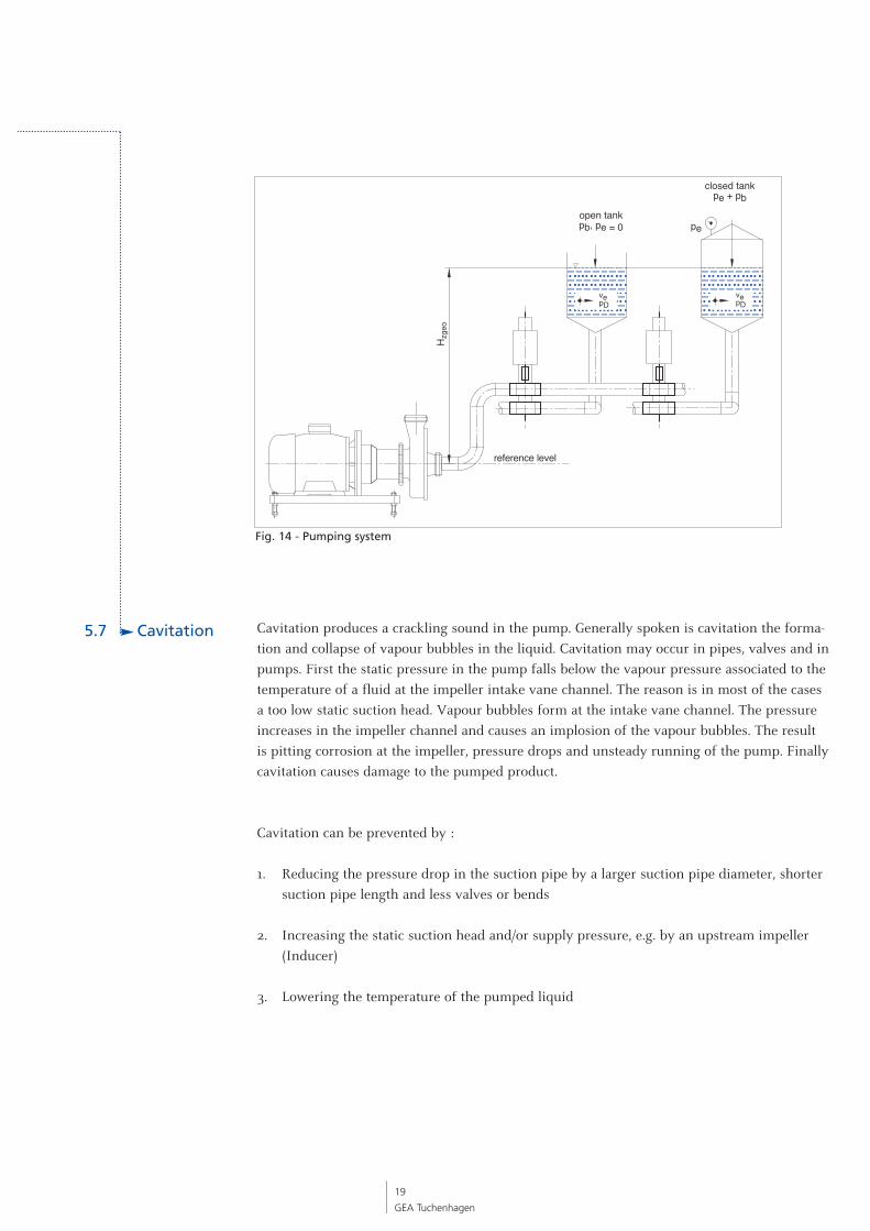
open tankpb, pe = 0
closed tankpe + pb
Hzg
eo
reference level
pe
vepDvepD
Fig. 14 - Pumping system
5.8 Q-H character-istic diagram
20
GEA Tuchenhagen
Before designing a pump, it is important to ascertain the characteristic curve of the plantthat allows you to select the right pump by help of the pump characteristic curve
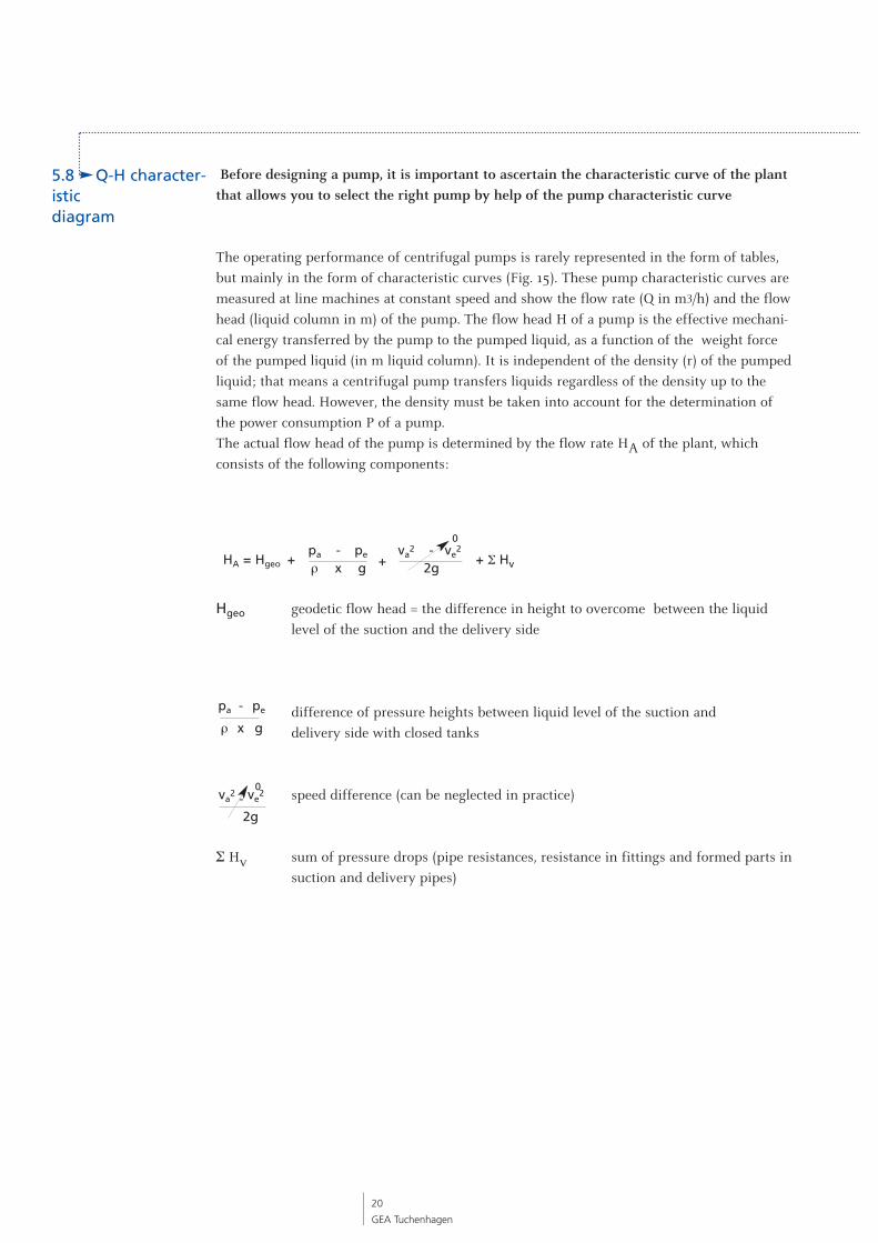
The operating performance of centrifugal pumps is rarely represented in the form of tables,but mainly in the form of characteristic curves (Fig. 15). These pump characteristic curves aremeasured at line machines at constant speed and show the flow rate (Q in m3/h) and the flowhead (liquid column in m) of the pump. The flow head H of a pump is the effective mechani-cal energy transferred by the pump to the pumped liquid, as a function of the weight forceof the pumped liquid (in m liquid column). It is independent of the density (r) of the pumpedliquid; that means a centrifugal pump transfers liquids regardless of the density up to thesame flow head. However, the density must be taken into account for the determination ofthe power consumption P of a pump.The actual flow head of the pump is determined by the flow rate HA of the plant, which consists of the following components:
Hgeo geodetic flow head = the difference in height to overcome between the liquidlevel of the suction and the delivery side
difference of pressure heights between liquid level of the suction and delivery side with closed tanks
speed difference (can be neglected in practice)
Σ Hv sum of pressure drops (pipe resistances, resistance in fittings and formed parts insuction and delivery pipes)
pa - pe
ρ x g
0va
2 - ve2
2g
0pa - pe va
2 - ve2
ρ x g 2gHA = Hgeo + + Σ Hv+
5.11 Plantcharacteristic curve
5.10 Flow head
5.9 Flow rate
5.12 Operating point
21
GEA Tuchenhagen
The flow rate (Q) accrues from the requirements of the process plant and is expressed in m3/hor GPM (Gallons per minute).
A decisive factor in designing a pump is the flow head (H), that depends on:
• the required flow head (for instance of a spray ball of 10 to 15 m;equal to 1.0 to 1.5 bar),
• difference in the pressure height of a liquid level on the delivery side and suction side,
• the sum of pressure drops caused by pipe resistance, resistance in components, fittings in the suction and delivery pipe.
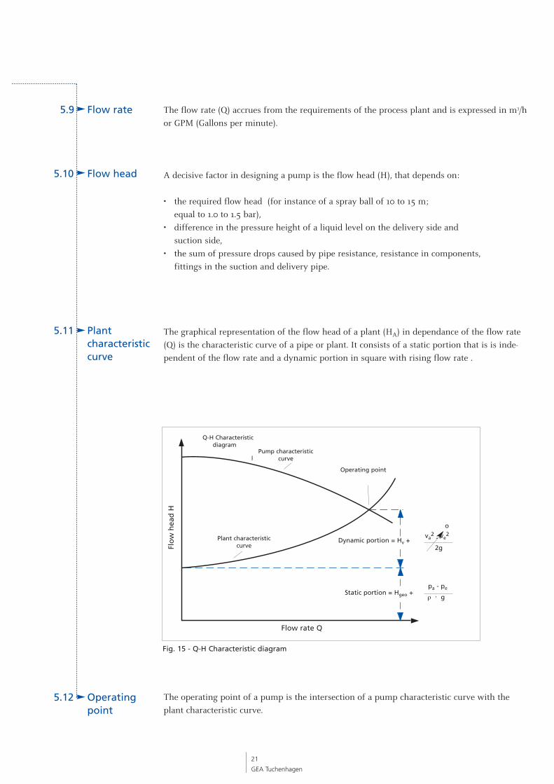
The graphical representation of the flow head of a plant (HA) in dependance of the flow rate(Q) is the characteristic curve of a pipe or plant. It consists of a static portion that is is inde-pendent of the flow rate and a dynamic portion in square with rising flow rate .
The operating point of a pump is the intersection of a pump characteristic curve with theplant characteristic curve.
Pumpenkennlinie
Anlagenkennlinie
Förderstrom Q
Förd
erh
öh
e H
Q-H Kennfeld
o
va2
- ve2
2g
pa - pe
ρ . g
Fig. 15 - Q-H Characteristic diagram
Operating point
Static portion = Hgeo +
Dynamic portion = Hv +
Q-H Characteristicdiagram
Pump characteristiccurve
Plant characteristiccurve
Flow rate Q
Flo
w h
ead
H

5.13 Pressure drops
22
GEA Tuchenhagen
Essential for the design of a pump are not only the NPSH, flow head and flow rate, butalso pressure drops.
Pressure drops of a plant may be caused by pressure drops in:• the pipe system,• installed components (valves, bends, inline measurement instruments),• installed process units (heat exchangers, spray balls).
Pressure drops Hv of the plant can be determined by help of tables and diagrams. Basis are the equations for pressure drops in pipes used for fluid mechanics that will not behandled any further.In view of extensive and time-consuming calculation work, it is recommended to proceed onthe example shown in Chapter 6.1. The tables in Chapter 8.2 and 8.3 help calculating the equi-valent pipe length. The data is based on a medium with a viscosity ν = 1 mm2/s (equal to water). Pressure drops for media with a higher viscosity can be converted using the diagrams in theannexed Chapter 8.5.
Various parmeters of the pipe system determine the pump design. Essential for the design ofthe pump is the required flow head. In the following, the three simplified theoritical calculati-on examples shall illustrate the complexity of this subject before in Chapter 6 the practicaldesign of a pump is handled.
Hv = Pressure dropHv,s = Total pressure drop - suction pipeHv,d = Total pressure drop - delivery pipeHs,geo = Geodetic head - suction pipeHz,geo = Geodetic head - supply pipeHd,geo = Geodetic head - delivery pipeHv,s = Pressure drop - suction pipeHv,d = Pressure drop - delivery pipep = Static pressure in the tank
Attention:Pressure in the tank or supplies in the suction pipe are negative because they must be deducted from the pressure drop. They intensify the flow.
5.14 Theoretical calculationexample
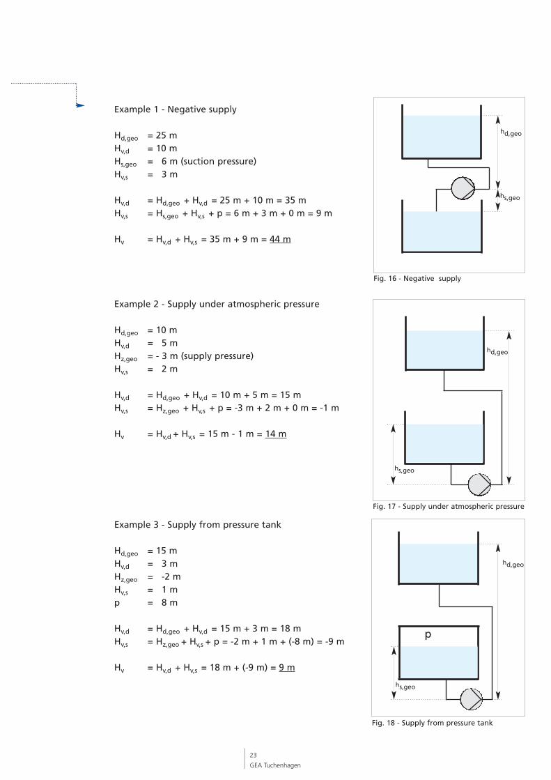
Example 1 - Negative supply
Hd,geo = 25 mHv,d = 10 mHs,geo = 6 m (suction pressure)Hv,s = 3 m
Hv,d = Hd,geo + Hv,d = 25 m + 10 m = 35 mHv,s = Hs,geo + Hv,s + p = 6 m + 3 m + 0 m = 9 m
Hv = Hv,d + Hv,s = 35 m + 9 m = 44 m
Example 2 - Supply under atmospheric pressure
Hd,geo = 10 mHv,d = 5 mHz,geo = - 3 m (supply pressure)Hv,s = 2 m
Hv,d = Hd,geo + Hv,d = 10 m + 5 m = 15 mHv,s = Hz,geo + Hv,s + p = -3 m + 2 m + 0 m = -1 m
Hv = Hv,d + Hv,s = 15 m - 1 m = 14 m
Example 3 - Supply from pressure tank
Hd,geo = 15 mHv,d = 3 mHz,geo = -2 mHv,s = 1 mp = 8 m
Hv,d = Hd,geo + Hv,d = 15 m + 3 m = 18 mHv,s = Hz,geo + Hv,s + p = -2 m + 1 m + (-8 m) = -9 m
Hv = Hv,d + Hv,s = 18 m + (-9 m) = 9 m
23
GEA Tuchenhagen
hd,geo
hd,geo
hs,geo
Fig. 16 - Negative supply
Fig. 17 - Supply under atmospheric pressure
hs,geo
Fig. 18 - Supply from pressure tank
hs,geo
p
hd,geo
Hv,s
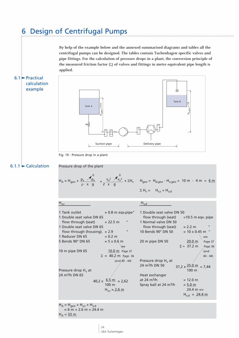
1 Tank outlet = 0.8 m eqv.pipe"1 Double seat valve DN 65
flow through (seat) = 22.5 m "1 Double seat valve DN 65
flow through (housing). = 2.9 "1 Reducer DN 65 = 0.2 m 5 Bends 90° DN 65 = 5 x 0.6 m
see
10 m pipe DN 65 10.0 m Page 37
Σ = 40.2 m Page 36
(and 40 - 44)
Pressure drop Hv at24 m3/h DN 65
6.5 m 100 m Hv,s = 2.6 m
Hv,d
1 Double seat valve DN 50 flow through (seat) =10.5 m eqv. pipe
1 Normal valve DN 50 flow through (seat) = 2.2 m "
10 Bends 90° DN 50 = 10 x 0.45 m "see
20 m pipe DN 50 20.0 m Page 37
Σ = 37.2 m Page 36
(and
40 - 44)
Pressure drop Hv at 24 m3/h DN 50 25.0 m
100 m Heat exchanger at 24 m3/h = 12.0 mSpray ball at 24 m3/h = 5.0 m
24.4 m =>Hv,d = 24.4 m
6.1.1 Calculation
6.1 Practical calculationexample
24
GEA Tuchenhagen
By help of the example below and the annexed summarised diagrams and tables all thecentrifugal pumps can be designed. The tables contain Tuchenhagen specific valves andpipe fittings. For the calculation of pressure drops in a plant, the conversion principle ofthe measured friction factor (ζ) of valves and fittings in metre equivalent pipe length isapplied.
6 Design of Centrifugal Pumps
Fig. 19 - Pressure drop in a plant
Pressure drop of the plant
HA = Hgeo + + ΣHv Hgeo = Hd,geo - Hz,geo = 10 m - 4 m = 6 m
Σ Hv = Hv,s + Hv,d
0 0
pa - pe va2 - ve
2
ρ x g 2 x g+
HA = Hgeo + Hv,s + Hv,d= 6 m + 2.6 m + 24.4 m
HA = 33 m
40,2 x = 2,62
37,2 x = 7,44
D DD
D
Hz,
geo
= 4
m
Hd
,geo
= 1
0
Saugleitung Druckleitung
Tank A
Tank B
Suction pipe Delivery pipe
The flow rate is 24 m3/h. Components and process units are installed in the pipe betweenTank A to be emptied and Tank B to be filled. As already mentioned before, it is essential toinstall the pump as close as possible to the tank to be emptied. Between Tank A and the pump are located a butterfly valve and two double seat valves aswell as one reducer and 5 bends and finally 10 m pipe in DN 65.
In the pipe from the pump up to Tank B (20 m in DN 50) are installed a double seat valve, asingle seat valve, one heat exchanger and one spray ball. The difference in elevation of theliquid level in Tank A to Tank B is 6 m. Now the metre equivalent pipe length must be deter-mined for each component installed. For this purpose see the standard tables for pressuredrops on Page 37 and 38. The outcome is in total 40.18 m on the suction side. This value isconverted into the corresponding pressure drop (H) of the pipe, cross section DN 65.According to the table, the pressure drop is 6.5 m per 100 m at a flow rate of 24 m3/h andwith a pipe DN 65. Based on 40.18 m, the pressure drop (Hv,s) is 2.61 m. Downstream thepump, the liquid must be conveyed in length equivalent pipe of 37.2 m in total. The pressuredrop of a pipe in DN 50 is according to the table 25 m per 100 m. Based on 37.2 m,the pressure drop is 7.4 m. In addition, on the delivery side there is a heat exchanger with apressure drop of 12 m (at 24 m3) as well as a spray ball at the end of the pipe with a pressuredrop of 5 m. In total the pressure drop on the delivery side (Hv,d) is 24.4 m.
The sum of pressure drops on the suction side (Hv,s), on the delivery side (Hv,d) and the geodetic flow head (Hgeo), result in a total pressure drop (HA) of 33.0 m that must be compensated by the pump.
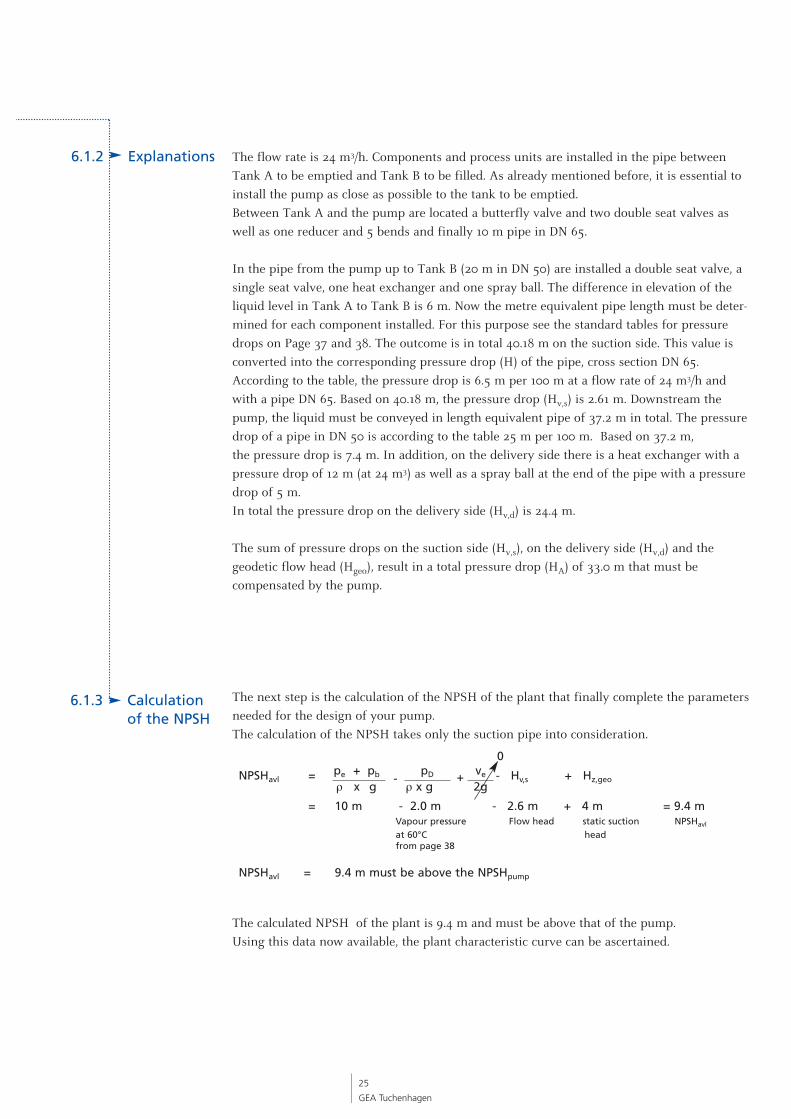
The next step is the calculation of the NPSH of the plant that finally complete the parametersneeded for the design of your pump.The calculation of the NPSH takes only the suction pipe into consideration.
NPSHavl = - Hv,s + Hz,geo
= 10 m - 2.0 m - 2.6 m + 4 m = 9.4 mVapour pressure Flow head static suction NPSHavl
at 60°C headfrom page 38
NPSHavl = 9.4 m must be above the NPSHpump
The calculated NPSH of the plant is 9.4 m and must be above that of the pump. Using this data now available, the plant characteristic curve can be ascertained.
6.1.3 Calculationof the NPSH
6.1.2 Explanations
25
GEA Tuchenhagen
0 pe + pb pD ve
ρ x g ρ x g 2g- +
6.2 Characteristic curve inter-pretation
26
GEA Tuchenhagen
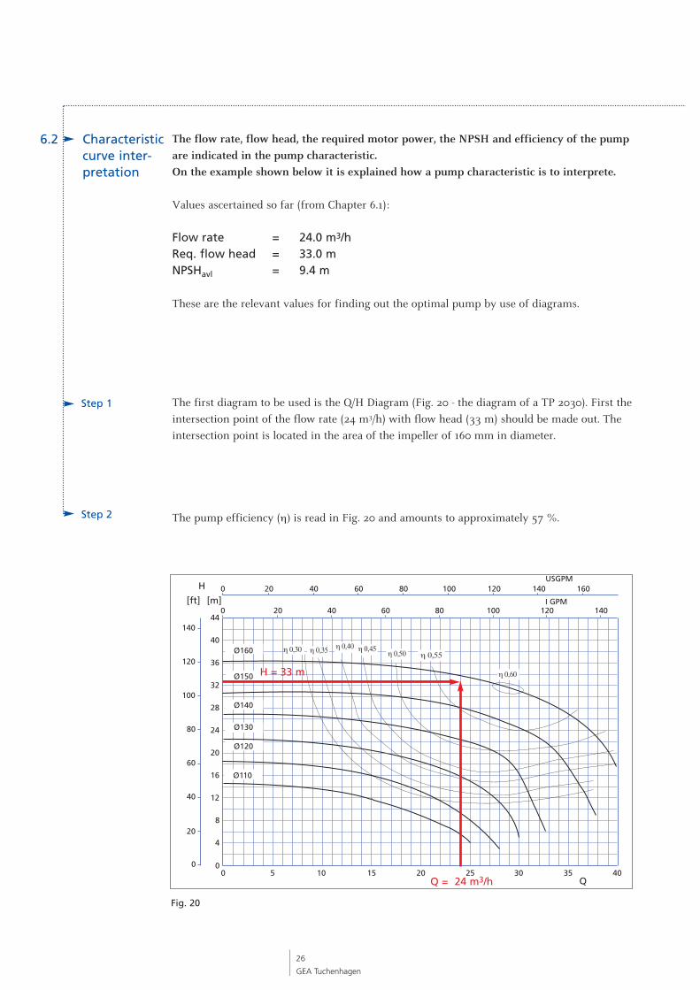
The flow rate, flow head, the required motor power, the NPSH and efficiency of the pumpare indicated in the pump characteristic. On the example shown below it is explained how a pump characteristic is to interprete.
Values ascertained so far (from Chapter 6.1):
Flow rate = 24.0 m3/hReq. flow head = 33.0 mNPSHavl = 9.4 m
These are the relevant values for finding out the optimal pump by use of diagrams.
The first diagram to be used is the Q/H Diagram (Fig. 20 - the diagram of a TP 2030). First theintersection point of the flow rate (24 m3/h) with flow head (33 m) should be made out. Theintersection point is located in the area of the impeller of 160 mm in diameter.
The pump efficiency (η) is read in Fig. 20 and amounts to approximately 57 %.
Step 1
H
44
40
36
32
28
24
20
16
12
8
4
[m][ft]
USGPM0
0
20 40 60 80 100 120 140
0 20 40 60 80 100 120
140
120
100
80
60
40
20
0
160
140
0 5 10 15 20 25 30 35Q
40
I GPM
Ø160
Ø150
Ø140
Ø130
Ø120
η 0,60
η 0,50η 0,45η 0,40η 0,35η 0,30
Ø110
η 0,55
Step 2
H = 33 m
Fig. 20
Q = 24 m3/h
27
GEA Tuchenhagen
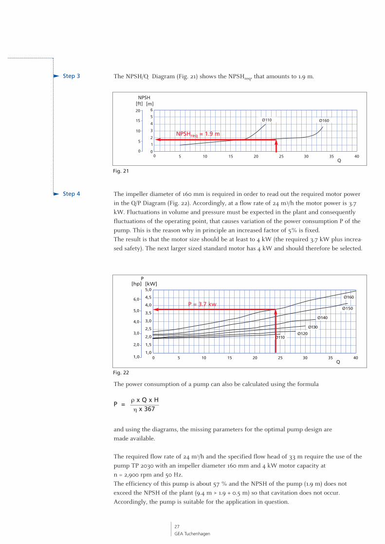
The NPSH/Q Diagram (Fig. 21) shows the NPSHreq, that amounts to 1.9 m.
The impeller diameter of 160 mm is required in order to read out the required motor powerin the Q/P Diagram (Fig. 22). Accordingly, at a flow rate of 24 m3/h the motor power is 3.7kW. Fluctuations in volume and pressure must be expected in the plant and consequentlyfluctuations of the operating point, that causes variation of the power consumption P of thepump. This is the reason why in principle an increased factor of 5% is fixed. The result is that the motor size should be at least to 4 kW (the required 3.7 kW plus increa-sed safety). The next larger sized standard motor has 4 kW and should therefore be selected.
The power consumption of a pump can also be calculated using the formula
P = ρ x Q x Hη x 367
and using the diagrams, the missing parameters for the optimal pump design are made available.
The required flow rate of 24 m3/h and the specified flow head of 33 m require the use of thepump TP 2030 with an impeller diameter 160 mm and 4 kW motor capacity at n = 2,900 rpm and 50 Hz. The efficiency of this pump is about 57 % and the NPSH of the pump (1.9 m) does notexceed the NPSH of the plant (9.4 m > 1.9 + 0.5 m) so that cavitation does not occur.Accordingly, the pump is suitable for the application in question.
Step 3
Step 4
[kW]
1,0
1,5
2,0
2,5
3,0
3,5
4,0
0 5 10 15 20 25 30 35Q
40
4,5
5,0
2,0
3,0
4,0
5,0
6,0
[hp]P
1,0
Ø160
Ø150
Ø140
Ø130
Ø120Ø110
NPSH[m]
0
[ft]
0
1
2
3
5 10 15 20 25 30 35Q
40
4
5
10
0
5
15
20 6
Ø110 Ø160
NPSHreq = 1.9 m
Fig. 21
Fig. 22
P = 3.7 kw
6.3 Modification
28
GEA Tuchenhagen
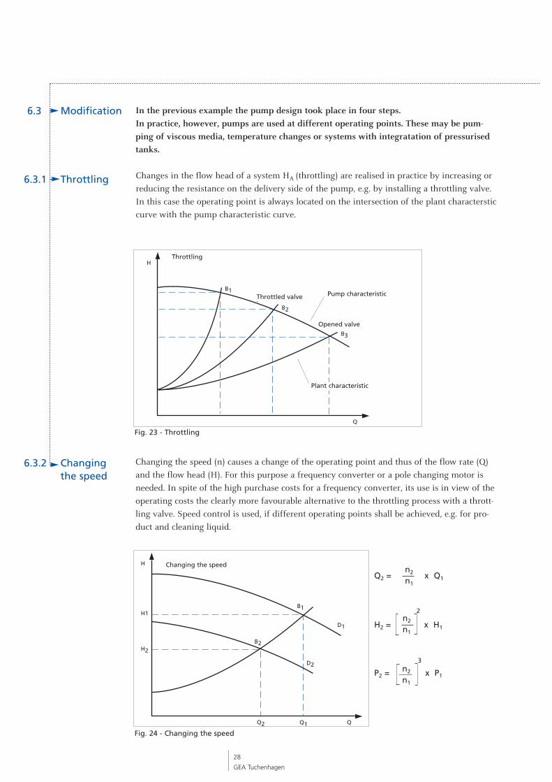
6.3.2 Changingthe speed
In the previous example the pump design took place in four steps. In practice, however, pumps are used at different operating points. These may be pum-ping of viscous media, temperature changes or systems with integratation of pressurisedtanks.
Changes in the flow head of a system HA (throttling) are realised in practice by increasing orreducing the resistance on the delivery side of the pump, e.g. by installing a throttling valve.In this case the operating point is always located on the intersection of the plant charactersticcurve with the pump characteristic curve.
Changing the speed (n) causes a change of the operating point and thus of the flow rate (Q)and the flow head (H). For this purpose a frequency converter or a pole changing motor isneeded. In spite of the high purchase costs for a frequency converter, its use is in view of theoperating costs the clearly more favourable alternative to the throttling process with a thrott-ling valve. Speed control is used, if different operating points shall be achieved, e.g. for pro-duct and cleaning liquid.
6.3.1 Throttling
H
B2
B1
Q
B3
gedrosseltes Ventil
geöffnetes Ventil
Drosselung
Pump characteristic
Plant characteristic
H2
H1
H
Q2 Q1 Q
D2
D1
B1
B2
Drehzahländerung
Q2 = x Q1n2
n1
H2 = x H1
n2
n1
2
P2 = x P1
3n2
n1
Fig. 23 - Throttling
Fig. 24 - Changing the speed
Throttling
Changing the speed
Throttled valve
Opened valve
6.3.5 Operation inseries
6.3.4 Operation inparallel
6.3.3 Reducing theimpeller size
29
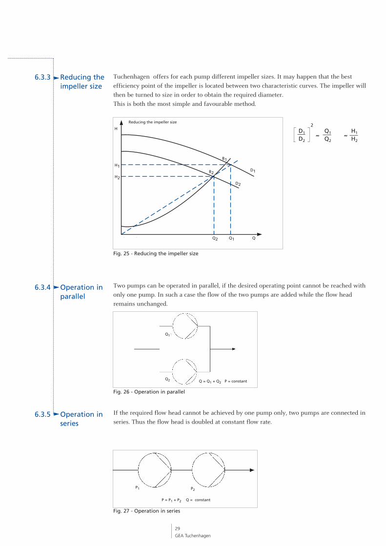
GEA Tuchenhagen
Tuchenhagen offers for each pump different impeller sizes. It may happen that the best efficiency point of the impeller is located between two characteristic curves. The impeller willthen be turned to size in order to obtain the required diameter. This is both the most simple and favourable method.
Two pumps can be operated in parallel, if the desired operating point cannot be reached withonly one pump. In such a case the flow of the two pumps are added while the flow headremains unchanged.
If the required flow head cannot be achieved by one pump only, two pumps are connected inseries. Thus the flow head is doubled at constant flow rate.
Q2 Q1 Q
H2
H1
H
D2
D1
B1
B2
picture 4
Impeller reduced
≈ ≈D1
D2
Q1
Q2
H1
H2
2
Fig. 25 - Reducing the impeller size
Fig. 26 - Operation in parallel
Fig. 27 - Operation in series
Q = Q1 + Q2 P = constant
Q1
Q2
P = P1 + P2 Q = constant
P1 P2
Reducing the impeller size

6.4.1 Correction forhigh viscosities
6.4 Pumping ofviscous media
30
GEA Tuchenhagen
In the previous example (Chapter 6.1) water served as pumping medium. In practice media other than water are conveyed. In this respect viscosity is a factor thatmust be taken into account for the calculation and design of the pump.
Conveying liquids of higher viscosity (ν) at constant speed (n), reduce the flow rate (Q), flowhead (H) and the efficiency (η) of the pump, while power consumption Pz of the pump (seeFig. 28) increases tt the same time. According to the method of approxima-tion, (6.4.2) the suitable pump size can be determined, starting from the operating point for viscous liquidsvia the operating point for water. The pump’s powerconsumption depends on the efficiency of the completeunit.
Annexed are tables used for the determination of pressure drops in dependence of viscosity and pipe diameter. In this connection it is worthwhile to menti-on that the pressure drop in dependence of viscosity isirrelevant for centrifugal pumps and can therefore beneglected. Centrifugal pumps are suitable for liquidsup to a viscosity of 500 mm2/s.If it is the question of pumping viscous media such asquarg, butter or syrup, rotary piston pumps will be used due to their higher efficiency in this respect.
The following page shows an example that explains the calculation and design of a pumpused for viscous media. Decisive in this connection are the correction factors for the flowhead (KH), flow rate (KQ) and the pump efficiency (Kη).
The correction factors are found in the diagram on page 31, by proceeding in the following steps:
1. Find out the kinematic viscosity of the medium in mm2/s2. Determine product of Q x √H (m3/h √m)3. Set up a vertical at the intersection of Q x √H with the corresponding viscosity4. Reading the intersections with the three correction lines at the vertical5. Enter these values into the equations and calculate the corrected value
On the basis of the obtained values, the pump can be desigend by means of the pump characteristic for water, (see Chapter 6.2).
H
Q
Hz
Pz
hz
P
h
picture 5
Fig. 28
31
GEA Tuchenhagen
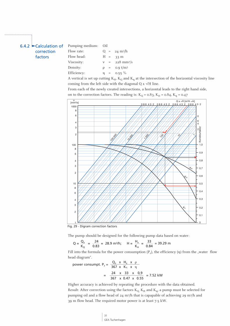
Pumping medium: Oil Flow rate: Q = 24 m3/hFlow head: H = 33 mViscosity: ν = 228 mm2/sDensity: ρ = 0.9 t/m3
Efficiency: η = 0.55 %A vertical is set up cutting KH, KQ and Kη at the intersection of the horizontal viscosity linecoming from the left side with the diagonal Q x √H line.From each of the newly created intersections, a horizontal leads to the right hand side, on to the correction factors. The reading is: KQ = 0.83, KH = 0.84, Kη = 0.47
The pump should be designed for the following pump data based on water:
Fill into the formula for the power consumption (Pz), the efficiency (η) from the „water flowhead diagram“.
Higher accuracy is achieved by repeating the procedure with the data obtained. Result: After correction using the factors KQ, KH and Kη, a pump must be selected for pumping oil and a flow head of 24 m3/h that is capapable of achieving 29 m3/h and 39 m flow head. The required motor power is at least 7.5 kW.
6.4.2 Calculation of correctionfactors
100.0
00
10.00
0
1.000 100 10 1
Kh
KQ
KH
1,0
0,9
0,8
0,7
0,6
0,5
0,4
0,3
0,2
0
0,1
2
46
0
0 8 6 4 3 2 0 8 6 4 3 2 0 8 6 4 3 2 0 8 6 4 3 2Q x ÷H [m3/h ÷m]
Korre
ktur
fakt
or
u[mm2/s]1000
8
6
4
3
2
108
6
4
3
2
1
1008
6
4
3
2
Qz 24 Hz 33KQ 0.83 KH 0.84
= 39.29 mQ = == = 28.9 m3/h; H =
Qz x Hz x ρ367 x Kη x η
power consumpt. Pz =
24 x 33 x 0,9
367 x 0.47 x 0.55= 7.52 kW=
Fig. 29 - Digram correction factors
7.1 Fundamentals
7.2 Pump ratingconditions
32
GEA Tuchenhagen
GEA Tuchenhagen Rotary Lobe Pumps of the VPSU and VPSH series are rotating positivedisplacement pumps. Two rotors with two lobes each rotate in the pump housing in oppo-site direction creating a fluid movement through the pump. The rotors do neither come in contact with each other nor with the pump housing.
A positive pressure difference is generated between the pump’s delivery and suction socketswhen the liquid is conveyed. A part of the pumped medium flows back from the delivery sideto the suction side through the gap between the two rotors and the pump housing. The flowrate - theoretically resulting from the volume of the working areas and the pump speed - isreduced by the volume of the back flow. The back flow portion rises with increasing deliverypressure and decreases as the product viscosity rises. The capacity limits of rotary lobe pumps are usually revealed when rating the pump. They arereached, if one of the parameters needed for the pump design cannot be determined (e.g.speed), or if the NPSH of the pump is above or equal to that of the plant. In such a case thenext bigger pump size should be selected for safety reasons.
Rotary lobe pumps, type VPSH and VPSU are positive displacement pumps. Pumping againsta closed delivery side will result in an intolerable rise of pressure that can destroy the pumpor other parts of the plant. If pumping against a closed delivery side cannot be excluded tothe full extent, safety measures are to be taken either by suitable flow path control or by theprovision of safety or overflow valves. GEA Tuchenhagen offers overflow valves of the VARIVENT® System, series "Q" that are either ready mounted (including by-pass from thedelivery to the suction side) or as a loose part for installa-tion on site.
In the following the rating of GEA Tuchenhagen rotary lobe pumps, type VPSH and VPSUshall be explained on an example.
For the selection of a pump that suits the specific application the following parametersshould be known:
Product data• Medium• Temperature• Product viscosity• Density• Portion of particles• Particle size
Pumping data• Volume flow Q in l/min.• Differential pressure ∆p in bar• NSPH of the plant in bar
7 Design of Rotary Lobe Pumps

33
GEA Tuchenhagen
7.3 Example Product data• Medium: Yeast• Temperature: t = 10°C• Viscosity: η = 100 cP• Density: ρ = 1,000 kg/m3
• Portion of particles none• Particle size none• Single acting mechanical seal in the pairing carbon against stainless steel
Pumping data• Q = 300 l/min.• ∆p = 5 bar• NPSH: 0.4 bar abs.
Selection of the pump size
The characteristic diagram (Fig. 30) may be used as a first step for the preliminary selection of the pump type in question. For this purpose the required flow rate and theknown viscosity of the product are to be entered. According to this diagram, the VPSH 54 isthe suit able pump size. Now the pump can be examined more closely using the detailed characteristic diagram (Fig. 31) shown on the next page.
1
10
100
1.000
10.000
100.000
1.000.000
1 10 100 1.000
4244
5254
6264
Fig. 30
Volume flow l/min
Vis
cosi
ty c
P
300 l/min
34
GEA Tuchenhagen
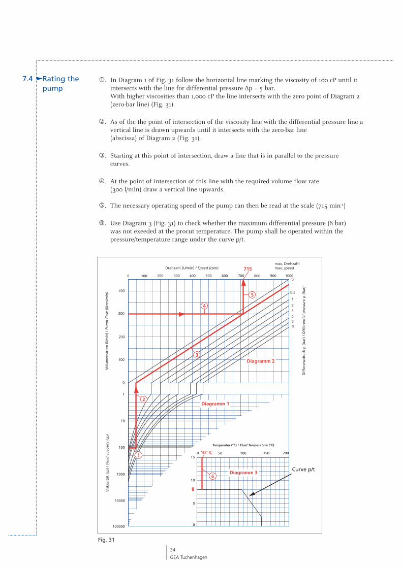
1. In Diagram 1 of Fig. 31 follow the horizontal line marking the viscosity of 100 cP until itintersects with the line for differential pres sure ∆p = 5 bar. With higher viscosities than 1,000 cP the line intersects with the zero point of Diagram 2(zero-bar line) (Fig. 31).
2. As of the the point of intersection of the viscosity line with the differential pressure line avertical line is drawn upwards until it intersects with the zero-bar line (abscissa) of Diagram 2 (Fig. 31).
3. Starting at this point of intersection, draw a line that is in parallel to the pressure curves.
4. At the point of intersection of this line with the required volume flow rate (300 l/min) draw a vertical line upwards.
5. The necessary operating speed of the pump can then be read at the scale (715 min-1)
6. Use Diagram 3 (Fig. 31) to check whether the maximum differential pressure (8 bar)was not exeeded at the procut temperature. The pump shall be operated within the pressure/temperature range under the curve p/t.
7.4 Rating the pump
1
10
100
1000
10000
100000
0 100 200 300 400 500 600 700 800 900 1000
0
5
10
15500 100 150 20010° C
8
0
100
200
300
400
865
3
2
1
0
0,55
4
3
2
1
6Diagramm 3
Diagramm 1
Diagramm 2
715Drehzahl (U/min) / Speed (rpm)
Vo
lum
enst
rom
(l/m
in)
/ Pu
mp
flo
w (
litre
s/m
in)
Dif
fere
nzd
ruck
p (
bar
) / D
iffe
ren
tial
pre
ssu
rep
(b
ar)
Vis
kosi
tät
(cp
) / F
luid
vis
cosi
ty (
cp)
Temperatur (°C) / Fluid Temperature (°C)
max. Drehzahlmax. speed
Fig. 31
Curve p/t

35
GEA Tuchenhagen
7. In diagram 4 (Fig. 32), first the viscosity factor required for calculat ing the capacity isdetermined by draw ing a vertical line upwards from the point of intersection of viscositywith the characteristic curve
8. and by reading the corres ponding viscosity factor f on the scale of the abscissa (2.8)
From the table in Diagram 4 (Fig. 32) find out factor S according to the selected gasket.
The required motor power is calculated as follows:
The required drive torque can now be calculated as follows:
9. From Diagram 5 (Fig. 32) the required pressure at the suction port (NSPHreq) can be read(intersection pump speed / viscosity). The pressure prevailing at the suction port (NPSHavl) should always be 0.1 bar higher than the required pres sure in order to prevent cavitation.
The result of the pump design is a VPSH 54 pump with a 3.0 kW motor and a pumpspeed of 750 rpm.
7.5 Result
pP (W) = 0.61
+ f + S x 0.265 x N( )
5P (W) = 0.61
+2,8 + 1 x 0.265 x 715
= 2.27 kW
( )
M (Nm) = 2270 x 9.56 = 30.35 Nm715
M (Nm) = P (W) x 9.56N
100.000
1.000.000
10.000
1.000
100
10
2 4 6 8 10 12 14 16 18 20 22 24 26
2,0
1,8
1,6
1,4
1,2
1,0
0,8
0,6
0,4
0,2
0100 200 300 400 500 600 700 800 900 1000 1100 1200 1300 1400 1500
NIPR
atmosphärischerDruck
atmosphericpressure
715
0,27
2,8
100.
000
cp
30.0
00 c
p
10.0
00 c
p
3.00
0 cp
1 cp10 cp100 cp
300 cp
1.000 cp
9
8
7
Diagramm 4
Diagramm 5
max. Drehzahl / max. speed
Pumpendrehzahl (U/min.) / Pump speed (rpm)
Viskositätsfaktor f / Viscosity factor f
erfo
rder
lich
er D
ruck
am
Sau
gst
utz
en (
bar
ab
s.)
net
inle
t p
ress
ure
req
uir
ed -
N.I.
P.R
. - (
bar
ab
solu
te)
Vis
kosi
tät
(cp
) / V
isco
sity
(cp
)
Dichtung Typ Code Faktor SSeal Type Code Factor SEinfach / Single C/SS 8 1Einfach / Single C/SIC 3 1Einfach / Single SIC/SIC 2 2Doppelt / Double C/SIC 4 2Doppelt / Double SIC/SIC 1 3
Kraftbedarf / Power Absorbed
pP (W) = 0.61
+ f + S x 0.455 x N
M (Nm) = P (W) x 9.56N
( )
p = Differenzdruck / Differential pressure (bar)N = Drehzahl (U/min) / Speed in rpmf = Viskositätsfaktor aus dem Diagramm /
Viscosity factor from graphS = Dichtung (siehe Tabelle) /
Seal factor from tableP = Leistung / Power (W)M = Drehmoment / Torque (Nm)
Technische Daten / Application DataMax. Wellendrehmoment / Max. input shaft torque (Nm) 150Max. radiale Wellenbelastung / Max. shaft radial load (N) 2250Max. Partikelgröße (weich) / Max. soft particle dia. (mm) 15Verdrängung / Displacement (cc/rev) 455Verdrängung / Displacement (litres/100revs) 45.5
Physikalische Daten / Physical DataGewicht der Pumpe ohne Antrieb / Bareshaft pump weight (kg) 35Ölvolumen / Oil capacity (cc) 1100Rückhaltevolumen / Hold up volume (cc) 820(horizontale Anschlüsse) / (horizontal ports)
Anzugsmomente / Tightening Torques (Nm)Enddeckelbolzen / End cover bolts 20Rotorschrauben / Rotor retainer screws 55Rotorgehäuseschrauben / Rotor case screws 20Getriebedeckelschrauben / Gear cover screws 15Zahnradmuttern / Gear nuts 100Rotorzugstangenschrauben VPSU / Rotor tie rod nuts 40
Rotortoleranzen / Rotor Clearances (mm)Vorne, Rotor zum Deckel / Front, rotor to end cover 0.15Radial, Rotor zum Rotorgehäuse / Radial, rotor to rotor case 0.25Rotor zu Rotor / Mesh, lobe to lobe - min 0.20
Fig. 32
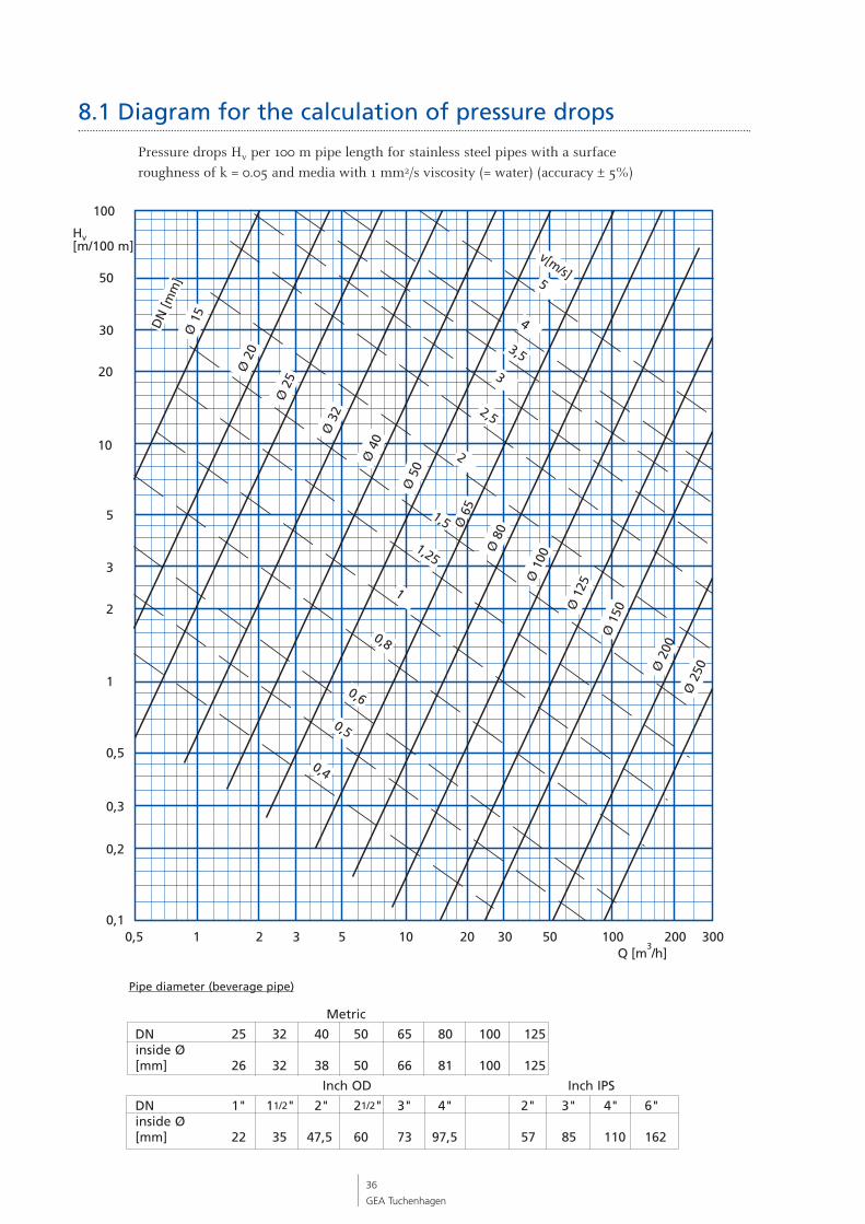
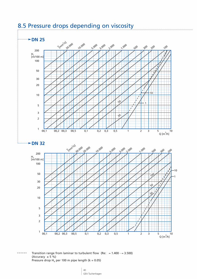
Pressure drops Hv per 100 m pipe length for stainless steel pipes with a surface roughness of k = 0.05 and media with 1 mm2/s viscosity (= water) (accuracy ± 5%)
Metric
DN 25 32 40 50 65 80 100 125inside Ø[mm] 26 32 38 50 66 81 100 125
Inch OD Inch IPS
DN 1" 11/2" 2" 21/2" 3" 4" 2" 3" 4" 6"inside Ø[mm] 22 35 47,5 60 73 97,5 57 85 110 162
36
GEA Tuchenhagen
8.1 Diagram for the calculation of pressure drops
100
50
30
20
10
5
3
2
0,5
1
0,3
0,2
0,10,5 1 2 3 5 10 20 30 50 100 300200
Hv[m/100 m]
Q [m3/h]
3
2,5
1
0,4
0,5
0,6
0,8
4
5
3,5
v[m/s]
Ø 1
5
2
1,5
Ø 2
50Ø 2
00
Ø 1
50Ø 1
25
Ø 1
00
Ø 8
0Ø 6
5
Ø 5
0
Ø 4
0
Ø 3
2
Ø 2
5
Ø 2
0
DN
[mm
]
1,25
Pipe diameter (beverage pipe)
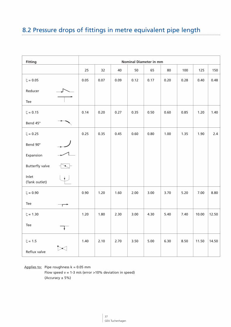
Fitting Nominal Diameter in mm
25 32 40 50 65 80 100 125 150
ζ = 0.05 0.05 0.07 0.09 0.12 0.17 0.20 0.28 0.40 0.48
Reducer
Tee
ζ = 0.15 0.14 0.20 0.27 0.35 0.50 0.60 0.85 1.20 1.40
Bend 45°
ζ = 0.25 0.25 0.35 0.45 0.60 0.80 1.00 1.35 1.90 2.4
Bend 90°
Expansion
Butterfly valve
Inlet
(Tank outlet)
ζ = 0.90 0.90 1.20 1.60 2.00 3.00 3.70 5.20 7.00 8.80
Tee
ζ = 1.30 1.20 1.80 2.30 3.00 4.30 5.40 7.40 10.00 12.50
Tee
ζ = 1.5 1.40 2.10 2.70 3.50 5.00 6.30 8.50 11.50 14.50
Reflux valve
37
GEA Tuchenhagen
8.2 Pressure drops of fittings in metre equivalent pipe length
Applies to: Pipe roughness k = 0.05 mm
Flow speed v = 1-3 m/s (error >10% deviation in speed)
(Accuracy ± 5%)
38
GEA Tuchenhagen
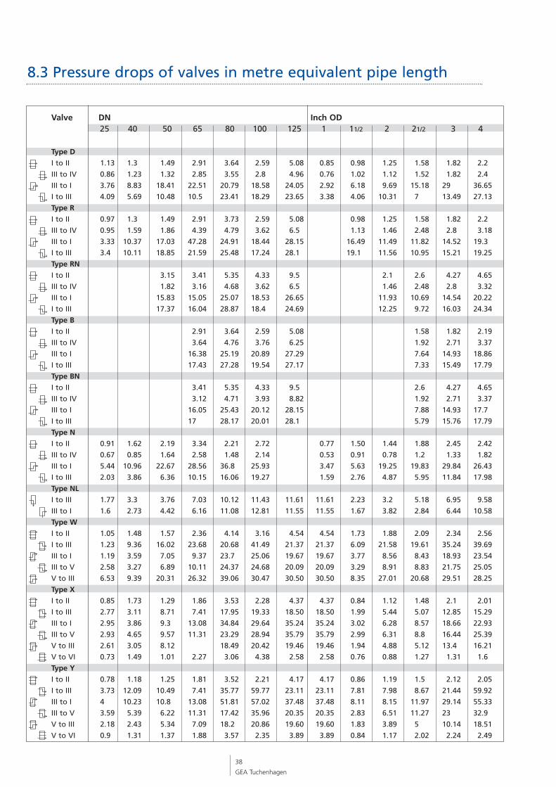
8.3 Pressure drops of valves in metre equivalent pipe length
Type D
I to II 1.13 1.3 1.49 2.91 3.64 2.59 5.08 0.85 0.98 1.25 1.58 1.82
III to IV 0.86 1.23 1.32 2.85 3.55 2.8 4.96 0.76 1.02 1.12 1.52 1.82
III to I 3.76 8.83 18.41 22.51 20.79 18.58 24.05 2.92 6.18 9.69 15.18 29
I to III 4.09 5.69 10.48 10.5 23.41 18.29 23.65 3.38 4.06 10.31 7 13.49
Type R
I to II 0.97 1.3 1.49 2.91 3.73 2.59 5.08 0.98 1.25 1.58 1.82
III to IV 0.95 1.59 1.86 4.39 4.79 3.62 6.5 1.13 1.46 2.48 2.8
III to I 3.33 10.37 17.03 47.28 24.91 18.44 28.15 16.49 11.49 11.82 14.52
I to III 3.4 10.11 18.85 21.59 25.48 17.24 28.1 19.1 11.56 10.95 15.21
Type RN
I to II 3.15 3.41 5.35 4.33 9.5 2.1 2.6 4.27
III to IV 1.82 3.16 4.68 3.62 6.5 1.46 2.48 2.8
III to I 15.83 15.05 25.07 18.53 26.65 11.93 10.69 14.54
I to III 17.37 16.04 28.87 18.4 24.69 12.25 9.72 16.03
Type B
I to II 2.91 3.64 2.59 5.08 1.58 1.82
III to IV 3.64 4.76 3.76 6.25 1.92 2.71
III to I 16.38 25.19 20.89 27.29 7.64 14.93
I to III 17.43 27.28 19.54 27.17 7.33 15.49
Type BN
I to II 3.41 5.35 4.33 9.5 2.6 4.27
III to IV 3.12 4.71 3.93 8.82 1.92 2.71
III to I 16.05 25.43 20.12 28.15 7.88 14.93
I to III 17 28.17 20.01 28.1 5.79 15.76
Type N
I to II 0.91 1.62 2.19 3.34 2.21 2.72 0.77 1.50 1.44 1.88 2.45
III to IV 0.67 0.85 1.64 2.58 1.48 2.14 0.53 0.91 0.78 1.2 1.33
III to I 5.44 10.96 22.67 28.56 36.8 25.93 3.47 5.63 19.25 19.83 29.84
I to III 2.03 3.86 6.36 10.15 16.06 19.27 1.59 2.76 4.87 5.95 11.84
Type NL
I to III 1.77 3.3 3.76 7.03 10.12 11.43 11.61 11.61 2.23 3.2 5.18 6.95
III to I 1.6 2.73 4.42 6.16 11.08 12.81 11.55 11.55 1.67 3.82 2.84 6.44
Type W
I to II 1.05 1.48 1.57 2.36 4.14 3.16 4.54 4.54 1.73 1.88 2.09 2.34
I to III 1.23 9.36 16.02 23.68 20.68 41.49 21.37 21.37 6.09 21.58 19.61 35.24
III to I 1.19 3.59 7.05 9.37 23.7 25.06 19.67 19.67 3.77 8.56 8.43 18.93
III to V 2.58 3.27 6.89 10.11 24.37 24.68 20.09 20.09 3.29 8.91 8.83 21.75
V to III 6.53 9.39 20.31 26.32 39.06 30.47 30.50 30.50 8.35 27.01 20.68 29.51
Type X
I to II 0.85 1.73 1.29 1.86 3.53 2.28 4.37 4.37 0.84 1.12 1.48 2.1
I to III 2.77 3.11 8.71 7.41 17.95 19.33 18.50 18.50 1.99 5.44 5.07 12.85
III to I 2.95 3.86 9.3 13.08 34.84 29.64 35.24 35.24 3.02 6.28 8.57 18.66
III to V 2.93 4.65 9.57 11.31 23.29 28.94 35.79 35.79 2.99 6.31 8.8 16.44
V to III 2.61 3.05 8.12 18.49 20.42 19.46 19.46 1.94 4.88 5.12 13.4
V to VI 0.73 1.49 1.01 2.27 3.06 4.38 2.58 2.58 0.76 0.88 1.27 1.31
Type Y
I to II 0.78 1.18 1.25 1.81 3.52 2.21 4.17 4.17 0.86 1.19 1.5 2.12
I to III 3.73 12.09 10.49 7.41 35.77 59.77 23.11 23.11 7.81 7.98 8.67 21.44
III to I 4 10.23 10.8 13.08 51.81 57.02 37.48 37.48 8.11 8.15 11.97 29.14
III to V 3.59 5.39 6.22 11.31 17.42 35.96 20.35 20.35 2.83 6.51 11.27 23
V to III 2.18 2.43 5.34 7.09 18.2 20.86 19.60 19.60 1.83 3.89 5 10.14
V to VI 0.9 1.31 1.37 1.88 3.57 2.35 3.89 3.89 0.84 1.17 2.02 2.24
Valve DN Inch OD25 40 50 65 80 100 125 1 11/2 2 21/2 3 4
2.2
2.4
36.65
27.13
2.2
3.18
19.3
19.25
4.65
3.32
20.22
24.34
2.19
3.37
18.86
17.79
4.65
3.37
17.7
17.79
2.42
1.82
26.43
17.98
9.58
10.58
2.56
39.69
23.54
25.05
28.25
2.01
15.29
22.93
25.39
16.21
1.6
2.05
59.92
55.33
32.9
18.51
2.49
39
GEA Tuchenhagen
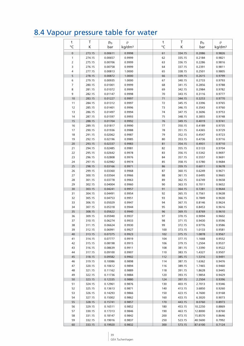
t T pD ρ t T pD ρ°C K bar kg/dm3 °C K bar kg/dm3
8.4 Vapour pressure table for water
0 273.15 0.00611 0.9998 61 334.15 0.2086 0.9826
1 274.15 0.00657 0.9999 62 335.15 0.2184 0.9821
2 275.15 0.00706 0.9999 63 336.15 0.2286 0.9816
3 276.15 0.00758 0.9999 64 337.15 0.2391 0.9811
4 277.15 0.00813 1.0000 65 338.15 0.2501 0.9805
5 278.15 0.00872 1.0000 66 339.15 0.2615 0.9799
6 279.15 0.00935 1.0000 67 340.15 0.2733 0.9793
7 280.15 0.01001 0.9999 68 341.15 0.2856 0.9788
8 281.15 0.01072 0.9999 69 342.15 0.2984 0.9782
9 282.15 0.01147 0.9998 70 343.15 0.3116 0.9777
10 283.15 0.01227 0.9997 71 344.15 0.3253 0.9770
11 284.15 0.01312 0.9997 72 345.15 0.3396 0.9765
12 285.15 0.01401 0.9996 73 346.15 0.3543 0.9760
13 286.15 0.01497 0.9994 74 347.15 0.3696 0.9753
14 287.15 0.01597 0.9993 75 348.15 0.3855 0.9748
15 288.15 0.01704 0.9992 76 349.15 0.4019 0.9741
16 289.15 0.01817 0.9990 77 350.15 0.4189 0.9735
17 290.15 0.01936 0.9988 78 351.15 0.4365 0.9729
18 291.15 0.02062 0.9987 79 352.15 0.4547 0.9723
19 292.15 0.02196 0.9985 80 353.15 0.4736 0.9716
20 293.15 0.02337 0.9983 81 354.15 0.4931 0.9710
21 294.15 0.02485 0.9981 82 355.15 0.5133 0.9704
22 295.15 0.02642 0.9978 83 356.15 0.5342 0.9697
23 296.15 0.02808 0.9976 84 357.15 0.5557 0.9691
24 297.15 0.02982 0.9974 85 358.15 0.5780 0.9684
25 298.15 0.03166 0.9971 86 359.15 0.6011 0.9678
26 299.15 0.03360 0.9968 87 360.15 0.6249 0.9671
27 300.15 0.03564 0.9966 88 361.15 0.6495 0.9665
28 301.15 0.03778 0.9963 89 362.15 0.6749 0.9658
29 302.15 0.04004 0.9960 90 363.15 0.7011 0.9652
30 303.15 0.04241 0.9957 91 364.15 0.7281 0.9644
31 304.15 0.04491 0.9954 92 365.15 0.7561 0.9638
32 305.15 0.04753 0.9951 93 366.15 0.7849 0.9630
33 306.15 0.05029 0.9947 94 367.15 0.8146 0.9624
34 307.15 0.05318 0.9944 95 368.15 0.8453 0.9616
35 308.15 0.05622 0.9940 96 369.15 0.8769 0.9610
36 309.15 0.05940 0.9937 97 370.15 0.9094 0.9602
37 310.15 0.06274 0.9933 98 371.15 0.9430 0.9596
38 311.15 0.06624 0.9930 99 372.15 0.9776 0.9586
39 312.15 0.06991 0.9927 100 373.15 1.0133 0.9581
40 313.15 0.07375 0.9923 102 375.15 1.0878 0.9567
41 314.15 0.07777 0.9919 104 377.15 1.1668 0.9552
42 315.15 0.08198 0.9915 106 379.15 1.2504 0.9537
43 316.15 0.08639 0.9911 108 381.15 1.3390 0.9522
44 317.15 0.09100 0.9907 110 383.15 1.4327 0.9507
45 318.15 0.09582 0.9902 112 385.15 1.5316 0.9491
46 319.15 0.10086 0.9898 114 387.15 1.6362 0.9476
47 320.15 0.10612 0.9894 116 389.15 1.7465 0.9460
48 321.15 0.11162 0.9889 118 391.15 1.8628 0.9445
49 322.15 0.11736 0.9884 120 393.15 1.9854 0.9429
50 323.15 0.12335 0.9880 124 397.15 2.2504 0.9396
51 324.15 0.12961 0.9876 130 403.15 2.7013 0.9346
52 325.15 0.13613 0.9871 140 413.15 3.6850 0.9260
53 326.15 0.14293 0.9866 150 423.15 4.7600 0.9168
54 327.15 0.15002 0.9862 160 433.15 6.3020 0.9073
55 328.15 0.15741 0.9857 170 443.15 8.0760 0.8973
56 329.15 0.16511 0.9852 180 453.15 10.2250 0.8869
57 330.15 0.17313 0.9846 190 463.15 12.8000 0.8760
58 331.15 0.18147 0.9842 200 473.15 15.8570 0.8646
59 332.15 0.19016 0.9837 250 523.15 40.5600 0.7992
60 333.15 0.19920 0.9832 300 573.15 87.6100 0.7124
40
GEA Tuchenhagen
Hv[m/100 m]
10
1
1
2
3
5
10
20
50
100
30
00,500,1 00,2 00,3 0,1 0,2 0,3 1 2 3 5 10
2001.000
2.00030.000
20.000
10.000
5.0003.000
Q [m3/h]
50
30
500300
0,5
200
100
[mm
2 /s]
υ
1
2
3
5
10
20
50
100
30
00,500,1 00,2 00,3 0,1 0,2 0,3 0,5 1 2 3 5 10
Hv[m/100 m]
2001.000
2.00010.000
5.0003.000
Q [m3/h]
500
50
300200
30
10
1
20.000
100[mm
2 /s]
υ
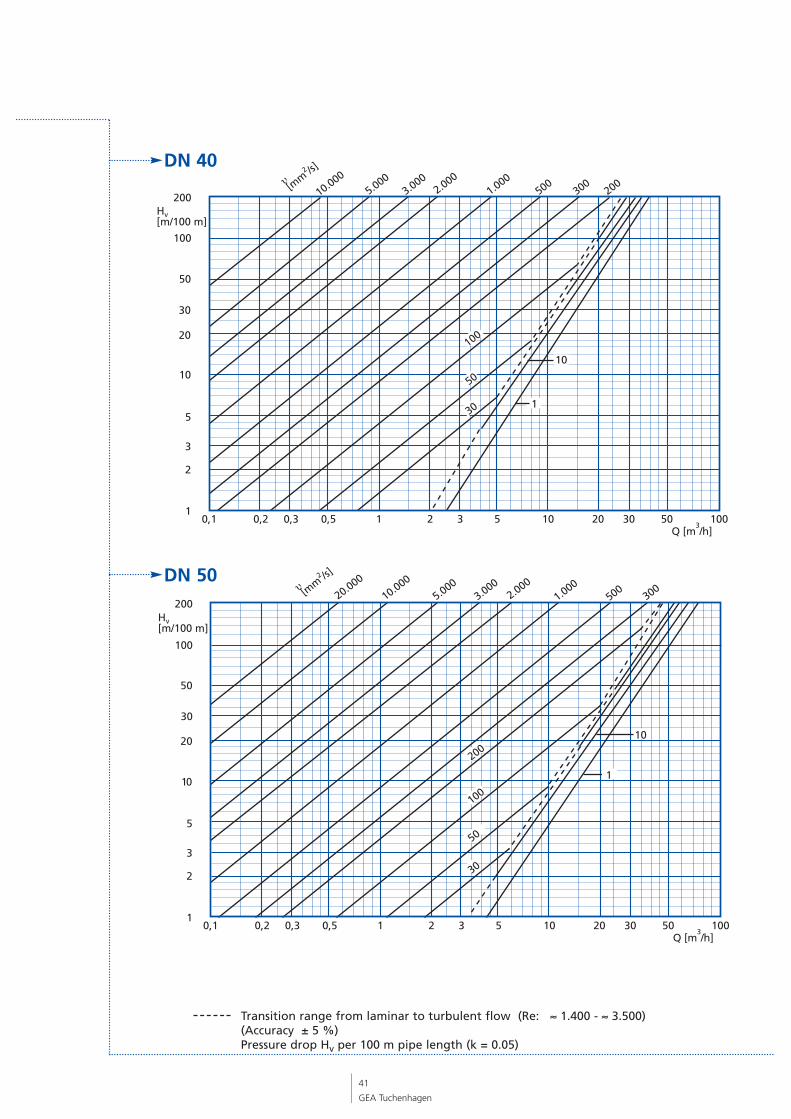
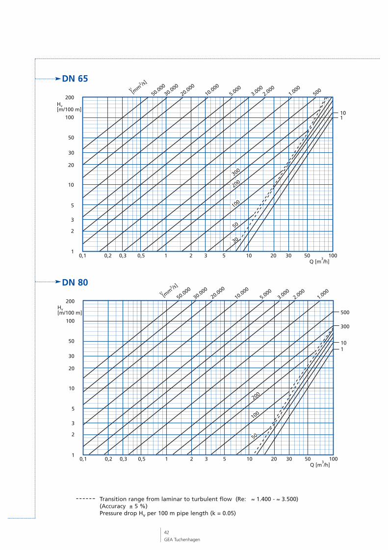
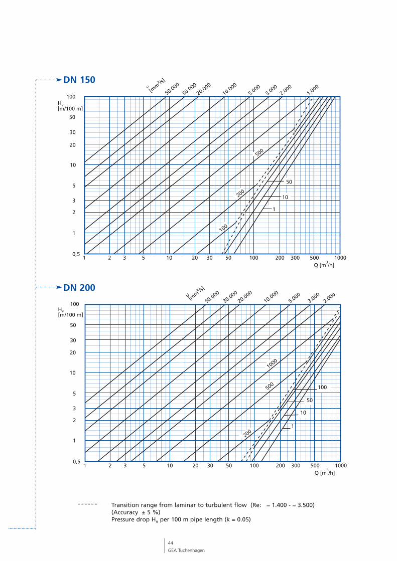
8.5 Pressure drops depending on viscosity
Transition range from laminar to turbulent flow (Re: ≈ 1.400 - ≈ 3.500)(Accuracy ± 5 %)Pressure drop Hv per 100 m pipe length (k = 0.05)
DN 32
DN 25
1
2
3
5
10
20
50
100
30
0,50,1 0,2 0,3 1 2 3 5 10 20 30 50 100
Hv[m/100 m]
200 1.0002.000
20.000
10.000
5.0003.000
Q [m3/h]
200
50
100
30
500300
1
10
[mm
2 /s]
υ
41
GEA Tuchenhagen
1
2
3
5
10
20
50
100
30
0,50,1 0,2 0,3 1 2 3 5 10 20 30 50 100
Hv[m/100 m]
200 1.0002.000
10.0005.000
3.000
Q [m3/h]
500
50
300200
100
30
10
1
[mm
2 /s]υ
Transition range from laminar to turbulent flow (Re: ≈ 1.400 - ≈ 3.500)(Accuracy ± 5 %)Pressure drop Hv per 100 m pipe length (k = 0.05)
DN 50
DN 40
42
GEA Tuchenhagen
1
2
3
5
10
20
50
100
30
0,50,1 0,2 0,3 1 2 3 5 10 20 30 50 100
Hv[m/100 m]
200 1.0002.000
50.000
30.000
20.000
10.000
5.0003.000
Q [m3/h]
500
300
200
100
50
30
101
[mm
2 /s]υ
Transition range from laminar to turbulent flow (Re: ≈ 1.400 - ≈ 3.500)(Accuracy ± 5 %)Pressure drop Hv per 100 m pipe length (k = 0.05)
DN 65
1
2
3
5
10
20
50
100
30
0,50,1 0,2 0,3 1 2 3 5 10 20 30 50 100
Hv[m/100 m]
2001.000
2.00050.000
30.00020.000
10.000
5.0003.000
Q [m3/h]
10
200
100
50
1
300
500
[mm
2 /s]
υ
DN 80

Hv[m/100 m]
50.000
30.000
20.000
10.000
5.0003.000
2.0001.000
1
2
3
5
10
20
50
100
30
0,50,1 0,2 0,3 0,5 1 2 3 5 10 20 30 50 100
Q [m3/h]
50
10
1
500
300
200
100
[mm
2 /s]υ
43
GEA Tuchenhagen
Transition range from laminar to turbulent flow (Re: ≈ 1.400 - ≈ 3.500)(Accuracy ± 5 %)Pressure drop Hv per 100 m pipe length (k = 0.05)
DN 100
1
2
3
5
10
20
50
100
30
0,50,1 0,2 0,3 0,5 1 2 3 5 10 20 30 50 100
3.0005.000
10.00020.000
50.000
Q [m3/h]
10
50
1
Hv[m/100 m]
200
300
500
1000
2000
100
30.000υ[m
m2 /s]DN 125
44
GEA Tuchenhagen
Hv[m/100 m]
50.000
30.000
20.000
10.000
5.0003.000
2.0001.000
1
2
3
5
10
20
50
100
30
0,51 2 3 5 10 20 30 50 100 200 300 500 1000
Q [m3/h]
500
200
100
50
10
1
[mm
2 /s]υ
1
2
3
5
10
20
50
100
30
0,51 2 3 5 10 20 30 50 100 200 300 500 1000
2.0003.000
5.00010.000
20.000
30.000
Q [m3/h]
1000
500
200
100
10
50
1
Hv[m/100 m]
50.000u[m
m2 /s]
Transition range from laminar to turbulent flow (Re: ≈ 1.400 - ≈ 3.500)(Accuracy ± 5 %)Pressure drop Hv per 100 m pipe length (k = 0.05)
DN 150
DN 200

45
GEA Tuchenhagen
Legal units (Abstract for centrifugal pumps)
Designation Formula Legal units not admitted Conversionsymbols (the unit listed first units
should be used)
Length l m base unit
km, cm, mm
Volume V m3 cbm, cdm
cm3, mm3, (Liter)
Flow rate Q m3/h
Volumetric flow V m3/s, I/s
Time t s (second) base unit
ms, min, h, d
Speed n 1/min
1/s
Mass m kg (Kilogram) pound, centner base unit
g, mg, (Tonne)
Density ρ kg/m3
kg/dm3, kg/cm3
Force F N (Newton = kg m/s2) kp, Mp 1 kp = 9.81 N
kN, mN
Pressure p bar (bar = N/m2) kp/cm2, at, 1 bar = 105 Pa = 0.1 MPaPa m WS, Torr, 1 at = 0.981 bar = 9.81 x 10⁴Pa
1 m WS = 0,98 bar
Energy, W, J (Joule = N m = W s) kp m 1 kp m = 9.81 JWort, Q kJ, Ws, kWh, kcal, cal 1 kcal = 4.1868 kJHeat amount 1 kWh = 3600 kJ
Flow head H m (Meter) m Fl.S.
Power P W (Watt = J/s = N m/s) kp m/s, PS 1 kp m/s = 9.81 W;MW, kW 1 PS = 736 W
Temperature, T K (Kelvin) °K, grd base unitt-difference °C
Kinematic ν m2/s St (Stokes), °E,… 1St = 10-4 m2/sviscosity mm2/s 1 cSt = 1 mm2/s
Approximation:mm2/s = (7.32 x °E - 6.31/°E)
ν =ηρ
Dynamic η Pa s (Pascal seconds = N s/m2) P (Poise), … 1P = 0.1 Pa sviscosity
8.6 SI - Units
46
GEA Tuchenhagen
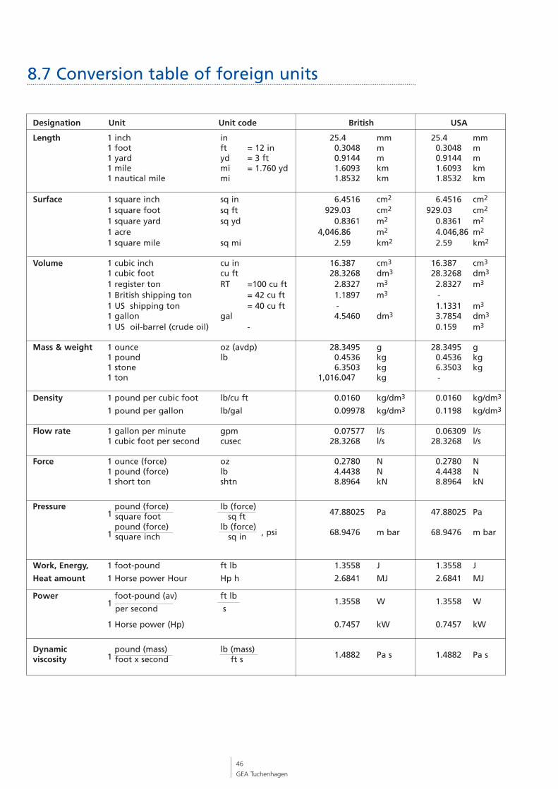
Length 1 inch in 25.4 mm 25.4 mm1 foot ft = 12 in 0.3048 m 0.3048 m1 yard yd = 3 ft 0.9144 m 0.9144 m1 mile mi = 1.760 yd 1.6093 km 1.6093 km1 nautical mile mi 1.8532 km 1.8532 km
Surface 1 square inch sq in 6.4516 cm2 6.4516 cm2
1 square foot sq ft 929.03 cm2 929.03 cm2
1 square yard sq yd 0.8361 m2 0.8361 m2
1 acre 4,046.86 m2 4.046,86 m2
1 square mile sq mi 2.59 km2 2.59 km2
Volume 1 cubic inch cu in 16.387 cm3 16.387 cm3
1 cubic foot cu ft 28.3268 dm3 28.3268 dm3
1 register ton RT =100 cu ft 2.8327 m3 2.8327 m3
1 British shipping ton = 42 cu ft 1.1897 m3 -1 US shipping ton = 40 cu ft - 1.1331 m3
1 gallon gal 4.5460 dm3 3.7854 dm3
1 US oil-barrel (crude oil) - 0.159 m3
Mass & weight 1 ounce oz (avdp) 28.3495 g 28.3495 g1 pound lb 0.4536 kg 0.4536 kg1 stone 6.3503 kg 6.3503 kg1 ton 1,016.047 kg -
Density 1 pound per cubic foot lb/cu ft 0.0160 kg/dm3 0.0160 kg/dm3
1 pound per gallon lb/gal 0.09978 kg/dm3 0.1198 kg/dm3
Flow rate 1 gallon per minute gpm 0.07577 l/s 0.06309 l/s1 cubic foot per second cusec 28.3268 l/s 28.3268 l/s
Force 1 ounce (force) oz 0.2780 N 0.2780 N1 pound (force) lb 4.4438 N 4.4438 N1 short ton shtn 8.8964 kN 8.8964 kN
Pressure1
pound (force) lb (force)47.88025 Pa 47.88025 Pasquare foot sq ft
1pound (force) lb (force)
, psi 68.9476 m bar 68.9476 m barsquare inch sq in
Work, Energy, 1 foot-pound ft lb 1.3558 J 1.3558 J
Heat amount 1 Horse power Hour Hp h 2.6841 MJ 2.6841 MJ
Power1
foot-pound (av) ft lb1.3558 W 1.3558 W
per second s
1 Horse power (Hp) 0.7457 kW 0.7457 kW
Dynamic1
pound (mass) lb (mass)1.4882 Pa s 1.4882 Pa sviscosity foot x second ft s
8.7 Conversion table of foreign units
Designation Unit Unit code British USA
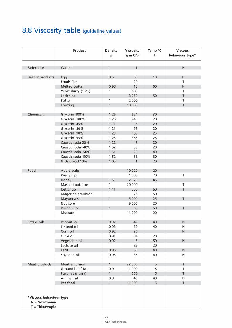
8.8 Viscosity table (guideline values)
47
GEA Tuchenhagen
Product Density Viscosity Temp °C Viscousρ η in CPs t behaviour type*
Reference Water 1 1 N
Bakery products Egg 0.5 60 10 N Emulsifier 20 TMelted butter 0.98 18 60 N Yeast slurry (15%) 1 180 TLecithine 3,250 50 TBatter 1 2,200 TFrosting 1 10,000 T
Chemicals Glycerin 100% 1.26 624 30Glycerin 100% 1.26 945 20Glycerin 45% 1.11 5 20Glycerin 80% 1.21 62 20Glycerin 90% 1.23 163 25Glycerin 95% 1.25 366 25Caustic soda 20% 1.22 7 20Caustic soda 40% 1.52 39 20Caustic soda 50% 1.51 20 40Caustic soda 50% 1.52 38 30Nictric acid 10% 1.05 1 20
Food Apple pulp 10,020 20Pear pulp 4,000 70 THoney 1.5 2,020 45Mashed potatoes 1 20,000 TKetschup 1.11 560 60 TMagarine emulsion 26 50Mayonnaise 1 5,000 25 TNut core 9,500 20Prune juice 1 60 50 TMustard 11,200 20
Fats & oils Peanut oil 0.92 42 40 NLinseed oil 0.93 30 40 NCorn oil 0.92 30 NOlive oil 0.91 84 20Vegetable oil 0.92 5 150 NLettuce oil 85 20Lard 0.96 60 40 NSoybean oil 0.95 36 40 N
Meat products Meat emulsion 1 22,000 5 TGround beef fat 0.9 11,000 15 TPork fat (slurry) 1 650 5 TAnimal fats 0.9 43 40 NPet food 1 11,000 5 T
*Viscous behaviour typeN = NewtonianT = Thixotropic
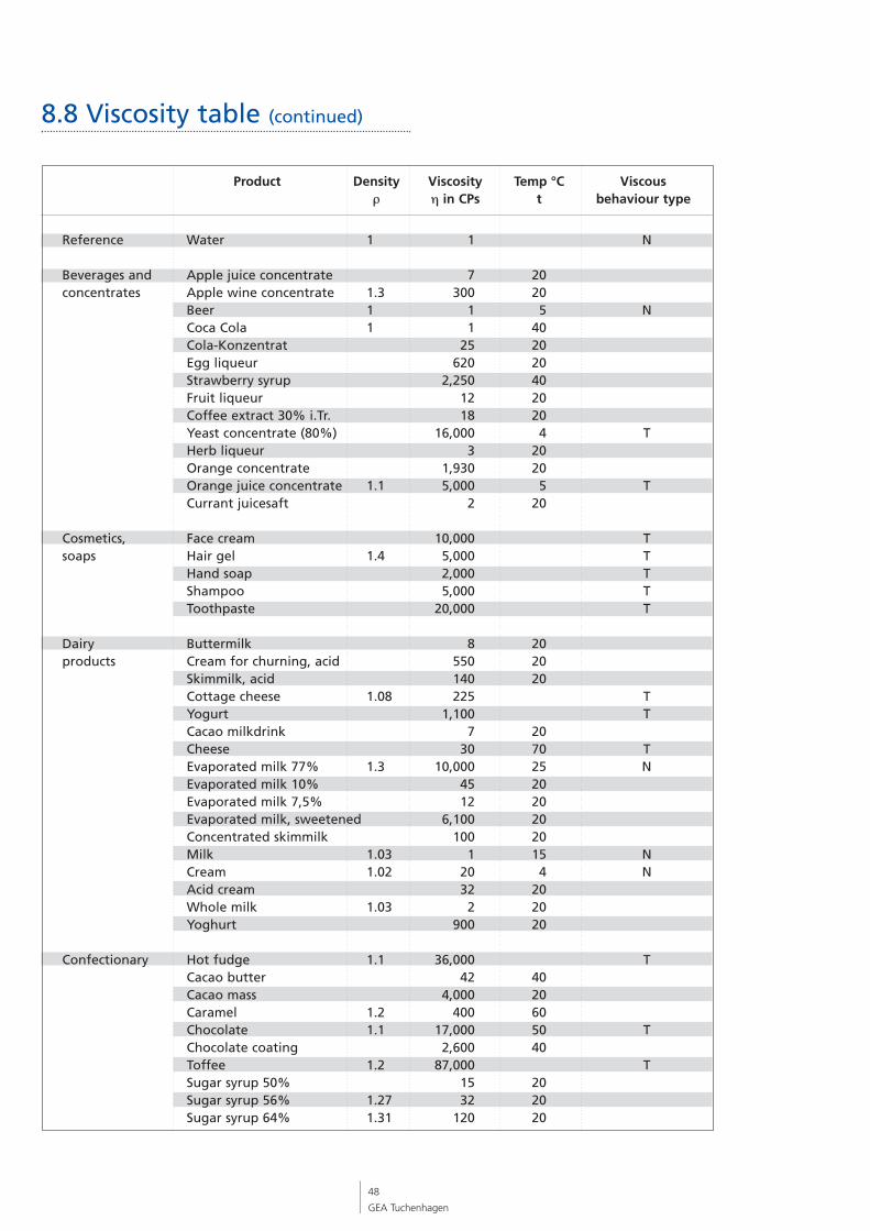
48
GEA Tuchenhagen
Product Density Viscosity Temp °C Viscous ρ η in CPs t behaviour type
8.8 Viscosity table (continued)
Reference Water 1 1 N
Beverages and Apple juice concentrate 7 20concentrates Apple wine concentrate 1.3 300 20
Beer 1 1 5 NCoca Cola 1 1 40Cola-Konzentrat 25 20Egg liqueur 620 20Strawberry syrup 2,250 40Fruit liqueur 12 20Coffee extract 30% i.Tr. 18 20Yeast concentrate (80%) 16,000 4 THerb liqueur 3 20Orange concentrate 1,930 20Orange juice concentrate 1.1 5,000 5 TCurrant juicesaft 2 20
Cosmetics, Face cream 10,000 Tsoaps Hair gel 1.4 5,000 T
Hand soap 2,000 TShampoo 5,000 TToothpaste 20,000 T
Dairy Buttermilk 8 20products Cream for churning, acid 550 20
Skimmilk, acid 140 20Cottage cheese 1.08 225 TYogurt 1,100 TCacao milkdrink 7 20Cheese 30 70 TEvaporated milk 77% 1.3 10,000 25 N Evaporated milk 10% 45 20Evaporated milk 7,5% 12 20Evaporated milk, sweetened 6,100 20Concentrated skimmilk 100 20Milk 1.03 1 15 NCream 1.02 20 4 NAcid cream 32 20Whole milk 1.03 2 20Yoghurt 900 20
Confectionary Hot fudge 1.1 36,000 TCacao butter 42 40Cacao mass 4,000 20Caramel 1.2 400 60Chocolate 1.1 17,000 50 TChocolate coating 2,600 40Toffee 1.2 87,000 TSugar syrup 50% 15 20Sugar syrup 56% 1.27 32 20Sugar syrup 64% 1.31 120 20
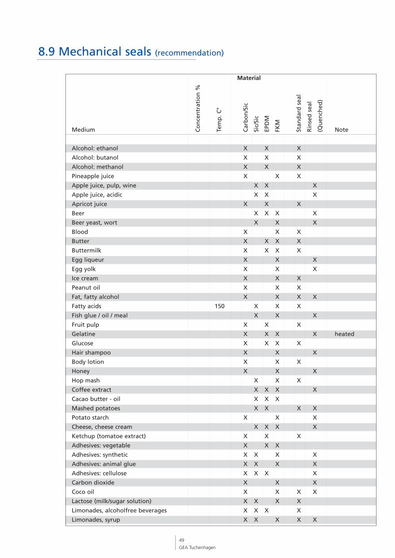
49
GEA Tuchenhagen
Co
nce
ntr
atio
n %
Tem
p. C
°
Car
bo
n/S
ic
Sic/
Sic
EPD
M
FKM
Stan
dar
d s
eal
Rin
sed
sea
l
(Qu
ench
ed)
Medium Note
Alcohol: ethanol X X X
Alcohol: butanol X X X
Alcohol: methanol X X X
Pineapple juice X X X
Apple juice, pulp, wine X X X
Apple juice, acidic X X X
Apricot juice X X X
Beer X X X X
Beer yeast, wort X X X
Blood X X X
Butter X X X X
Buttermilk X X X X
Egg liqueur X X X
Egg yolk X X X
Ice cream X X X
Peanut oil X X X
Fat, fatty alcohol X X X X
Fatty acids 150 X X X
Fish glue / oil / meal X X X
Fruit pulp X X X
Gelatine X X X X heated
Glucose X X X X
Hair shampoo X X X
Body lotion X X X
Honey X X X
Hop mash X X X
Coffee extract X X X X
Cacao butter - oil X X X
Mashed potatoes X X X X
Potato starch X X X
Cheese, cheese cream X X X X
Ketchup (tomatoe extract) X X X
Adhesives: vegetable X X X
Adhesives: synthetic X X X X
Adhesives: animal glue X X X X
Adhesives: cellulose X X X X
Carbon dioxide X X X
Coco oil X X X X
Lactose (milk/sugar solution) X X X X
Limonades, alcoholfree beverages X X X X
Limonades, syrup X X X X X
8.9 Mechanical seals (recommendation)
Material
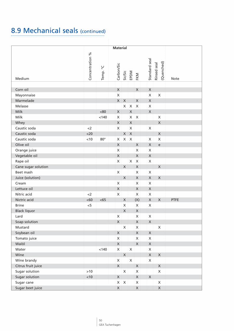
Medium Note
Corn oil X X X
Mayonnaise X X X
Marmelade X X X X
Melasse X X X X
Milk <80 X X X
Milk <140 X X X X
Whey X X X
Caustic soda <2 X X X
Caustic soda <20 X X X
Caustic soda <10 80° X X X X X
Olive oil X X X e
Orange juice X X X
Vegetable oil X X X
Rape oil X X X X
Cane sugar solution X X X
Beet mash X X X
Juice (solution) X X X X
Cream X X X
Lettuce oil X X X
Nitric acid <2 X X X
Nictric acid <60 <65 X (X) X X PTFE
Brine <5 X X X
Black liquor X X
Lard X X X
Soap solution X X X
Mustard X X X
Soybean oil X X X
Tomato juice X X X
Walöl X X X
Water <140 X X X
Wine X X X
Wine brandy X X X
Citrus fruit juice X X X
Sugar solution >10 X X X
Sugar solution <10 X X X
Sugar cane X X X X
Sugar beet juice X X X
50
GEA Tuchenhagen
8.9 Mechanical seals (continued)
Co
nce
ntr
atio
n %
Tem
p. °
C
Car
bo
n/S
ic
Sic/
Sic
EPD
M
FKM
Stan
dar
d s
eal
Rin
sed
sea
l
(Qu
ench
ed)
Material
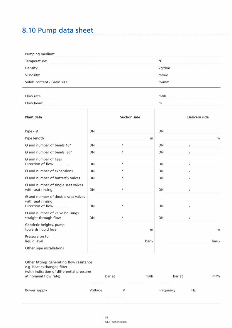
51
GEA Tuchenhagen
Pumping medium:
Temperature: °C
Density: kg/dm3
Viscosity: mm2/s
Solids content / Grain size: %/mm
Flow rate: m3/h
Flow head: m
Plant data Suction side Delivery side
Pipe - Ø DN DN
Pipe length m m
Ø and number of bends 45° DN / DN /
Ø and number of bends 90° DN / DN /
Ø and number of TeesDirection of flow…………… DN / DN /
Ø and number of expansions DN / DN /
Ø and number of butterfly valves DN / DN /
Ø and number of single seat valveswith seat rinsing DN / DN /
Ø and number of double seat valveswith seat rinsingDirection of flow…………… DN / DN /
Ø and number of valve housingsstraight through flow DN / DN /
Geodetic heights, pumptowards liquid level m m
Pressure on to liquid level barG barG
Other pipe installations
Other fittings generating flow resistancee.g. heat exchanger, filter(with indication of differential pressuresat nominal flow rate) bar at m3/h bar at m3/h
Power supply Voltage V Frequency Hz
8.10 Pump data sheet
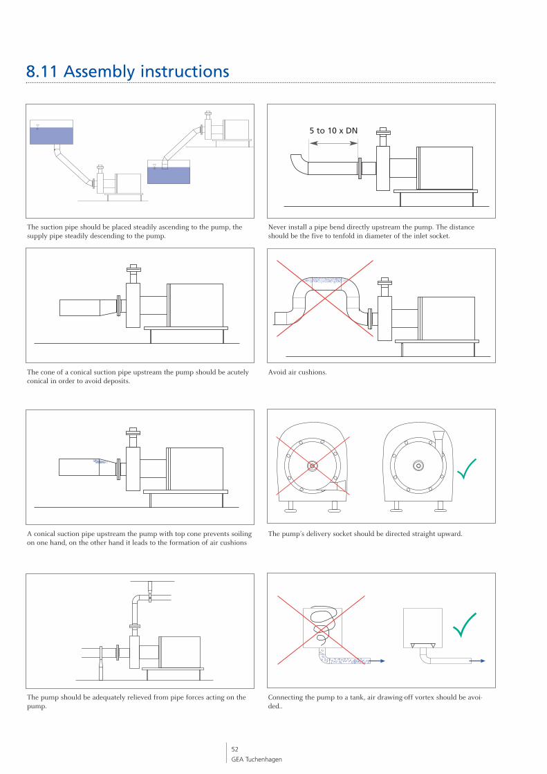
52
GEA Tuchenhagen
8.11 Assembly instructions
5 to 10 x DN
The suction pipe should be placed steadily ascending to the pump, thesupply pipe steadily descending to the pump.
Never install a pipe bend directly upstream the pump. The distanceshould be the five to tenfold in diameter of the inlet socket.
The cone of a conical suction pipe upstream the pump should be acutelyconical in order to avoid deposits.
Avoid air cushions.
A conical suction pipe upstream the pump with top cone prevents soilingon one hand, on the other hand it leads to the formation of air cushions
The pump’s delivery socket should be directed straight upward.
The pump should be adequately relieved from pipe forces acting on thepump.
Connecting the pump to a tank, air drawing-off vortex should be avoi-ded..

53
GEA Tuchenhagen
Notes

54
GEA Tuchenhagen
Noties

55
GEA Tuchenhagen

608e
-05/
2012
GEA Mechanical Equipment
GEA Tuchenhagen GmbH
Am Industriepark 2-10, 21514 BüchenPhone +49-4155 49-0, Fax +49- 04155 [email protected], www.tuchenhagen.com
Excellence Passion Integrity Responsibility GEA-versity
GEA Group is a global mechanical engineering company with multi-billion euro sales and operationsin more than 50 countries. Founded in 1881 the company is one of the largest providers of innovative equipment and process technology. GEA Group is listed in the STOXX Europe 600 Index.