manual flychk nov08 - nistnlte.nist.gov/fly/doc/manual_flychk_nov08.pdfthe manual for fly is already...
TRANSCRIPT

The How To
For
FLYCHK
@ NIST
H. K. Chung1
R. W. Lee
M. H. Chen
Y. Ralchenko
November 2008
1 Contact [email protected] for further questions on this material

FLYCHK............................................................................................................................................................... 1 I) INTRODUCTION ....................................................................................................................................... 4 II) THEORETICAL PLASMA SPECTROSCOPY .................................................................................. 5 A. PLASMA MODELS...................................................................................................................................... 5
(1) TE (THERMODYNAMIC EQUILIBRIUM) MODEL ......................................................................................... 5 (2) LTE (LOCAL THERMODYNAMIC EQUILIBRIUM) MODEL .......................................................................... 6 (3) CORONAL MODEL........................................................................................................................................ 7 (4) CR (COLLISIONAL-RADIATIVE) MODEL .................................................................................................... 7
B. COLLISIONAL-RADIATIVE MODEL (NON-LTE MODEL)............................................................ 8 (1) BACKGROUND.............................................................................................................................................. 8 (2) FORMULATION OF COLLISIONAL-RADIATIVE MODEL ............................................................................. 11
a) Formulation of Rate Equations ............................................................................................................ 11 b) Formulation of Radiation Transport Equation ................................................................................... 12
C. SPECTROSCOPIC ANALYSIS ................................................................................................................ 17 (1) SPECTRAL INTENSITY ANALYSIS .............................................................................................................. 17 (2) LINE BROADENING ANALYSIS .................................................................................................................. 20
a) Doppler Broadening ............................................................................................................................21 b) Stark Broadening................................................................................................................................... 21 C. Observed Line Profiles (Voigt Profile)................................................................................................22
III) THE MODEL DESCRIPTION................................................................................................................ 23 A. GENERAL DESCRIPTION....................................................................................................................... 23 B. ATOMIC DATA ........................................................................................................................................... 25
(1) ENERGY LEVELS........................................................................................................................................ 25 (2) RADIATIVE PROCESSES .............................................................................................................................27 (3) COLLISIONAL PROCESSES ......................................................................................................................... 28 (4) AUTOIONIZATION AND ELECTRON CAPTURE ............................................................................................31
C. PLASMA EFFECTS .................................................................................................................................... 32 (1) IONIZATION POTENTIAL DEPRESSION....................................................................................................... 32 (2) HIGH N STATES ......................................................................................................................................... 33 (3) ELECTRON ENERGY DISTRIBUTION FUNCTION ........................................................................................ 34 (4) OPACITY EFFECTS...................................................................................................................................... 34 (5) DILUTION OF THE RADIATION FIELD ........................................................................................................ 35
D. KINETICS MODELS.................................................................................................................................. 35 (1) LTE SOLUTION.......................................................................................................................................... 36 (2) NON-LTE STEADY-STATE SOLUTION IN OPTICALLY THIN LIMIT ......................................................... 37
A) rate Matrix ............................................................................................................................................ 37 B) Matrix inversion.................................................................................................................................... 37 C) Solution For Mixtures .......................................................................................................................... 38
(3) NON-LTE STEADY-STATE SOLUTION WITH OPTICAL DEPTH EFFECTS................................................. 39 A) Iteration Scheme For Ion Density........................................................................................................ 39 B) Approximation For Optical Depth Effects .......................................................................................... 40
(4) SOLUTION OF THE TIME-DEPENDENT RATE EQUATIONS......................................................................... 41 E. SPECTRUM GENERATION..................................................................................................................... 42
(1) GENERAL DESCRIPTION .............................................................................................................................42 (2) H, HE AND LI-LIKE IONS ...........................................................................................................................44

(3) ALL THE OTHER IONS................................................................................................................................. 45 (4) NIST ATOMIC SPECTRA DATA................................................................................................................... 46
IV) OUTLINE OF OPERATION ................................................................................................................... 47 A. INPUT COMMANDS.................................................................................................................................. 48
(1) FLYCHK ................................................................................................................................................... 48 a) z ..............................................................................................................................................................48 b) tr .............................................................................................................................................................48 c) ti ..............................................................................................................................................................49 d) opacity.................................................................................................................................................... 49 e) mixture.................................................................................................................................................... 50 f) fhot .......................................................................................................................................................... 50 g) fe .............................................................................................................................................................50 h) evolve ..................................................................................................................................................... 51 i) initial ....................................................................................................................................................... 51 j) history ..................................................................................................................................................... 51
• Using a hydrodynamic data file........................................................................................................................... 51 • Creating a grid of temperature and density ........................................................................................................ 52
• te ...................................................................................................................................................................... 52 • ne or nt or rho.................................................................................................................................................. 53
k) time ......................................................................................................................................................... 53 l) end ...........................................................................................................................................................53
(2) FLYSPEC.................................................................................................................................................. 53 B. OUTPUT ....................................................................................................................................................... 54
(1) FLYCHK ................................................................................................................................................... 54 A) SCREEN LOG FILE ....................................................................................................................................... 54 B) ENERGIES AND RATES FOR ATOMIC RATES ................................................................................................54 C) MAIN OUTPUT FILE .................................................................................................................................... 60 D) MEAN ION CHARGE .................................................................................................................................... 62 E) ION STAGE DISTRIBUTIONS ........................................................................................................................ 62 (2) FLYSPEC.................................................................................................................................................. 62

I) INTRODUCTION Recently, there has been a resurgence in the development of novel plasma-generation: x-ray lasers, ultra-short-pulse lasers, NIF(National Ignition Facility) and powerful z-pinch machines and there is an enhanced opportunity for the study of novel plasmas using the techniques associated with plasma spectroscopy. While the K-shell based spectroscopic code suite FLY, and its predecessors, have been successfully employed to study hot dense plasmas for decades, the emphasis of the new plasma generation schemes are moving into uncharted parts of the Temperature-Density phase-space: warm dense matter, highly transient states of matter, and extremely hot and dense matter. To provide a straightforward tool to help experimental design and spectral analysis, we have developed a suite of codes consistent with the philosophy used to develop the older FLY suite of codes: simple, easy-to-use, fast, portable and providing sufficiently reasonable spectroscopy for most users to have a design and analysis tool. The purpose of this manual is to provide the reader with enough information on the plasma spectroscopy to be able to use and understand the new suite of computer codes called FLYCHK currently available at the NIST Atomic Spectroscopy website http://nlte.nist.gov/FLY. There exist the on-line description of how to use the code and example files for various applications and yet the more detailed description of the code is warranted for understanding the results in depth. The manual for FLY is already available and gives a reasonable idea about how to go about designing and/or analyzing experiments where single-electron spectrum is to be observed. This manual for FLYCHK is focused in presenting the details of plasma population kinetics models contained in FLYCHK and compliments the FLY manual. Therefore users are strongly suggested to read both manuals. In the section II, we gives an introduction of theoretical plasma spectroscopy models as a brief summary of what is required in generating spectra : plasma kinetics models, particularly, collisional-radiative model, aka, non-LTE model and a radiative transport theory. Also presented are the simple methods of spectral analysis: spectral intensity analysis and line broadening analysis widely used in the community. In the section III, specific details of the code are given such as assumptions of the model, atomic data generation and methods to generate synthetic spectra. In the section IV, the operation of the code is outlined and users interested in a quick start may read this section first. The detailed discussion on the output files is given as well. Finally, in the section V, a few examples of interesting problems in laboratory experiment conditions are presented. Running the code does not require any atomic data input since the data is stored internally and read from the given file. The only thing the user must provide is the atomic element to be studied and some rough idea of the plasma conditions of interest. The inputs are kept to a minimum so that the user can extract as much information as possible without difficulty. This approach is dictated by an interest in making the analysis of experiments as straightforward as possible.

II) THEORETICAL PLASMA SPECTROSCOPY
A. Plasma Models The knowledge of atomic level population distributions of particles in a plasma is the key step for quantifying plasma parameters such as internal energy, partition function, opacity or equation of state. It is especially important in the analysis of observed spectra as a plasma diagnostic. A level population distribution of atoms in a plasma is closely related to thermodynamic parameters such as plasma temperature and density. Plasma models are reviewed which describe population kinetics under certain thermodynamic conditions1.
(1) TE (THERMODYNAMIC EQUILIBRIUM) MODEL The thermodynamic equilibrium (TE) model describes an equilibrium state of a plasma, where the rate of each and every atomic process is exactly balanced by the rate of its inverse process. Each atomic process is said to be in detailed balance. In the TE model, a physical state of the plasma can be completely expressed by a finite number of thermodynamic variables such as density and temperature. At temperature T, atomic level population distributions are determined from Boltzmann statistics and Saha ionization distribution. A level population density of level i in atoms of ionization state z can be written according to Boltzmann distribution,
!
niz =Nz
Uz (T)giz exp "
Eiz
kT
#
$ % &
' (
where Nz is the total number of ion z, giz is the statistical weight assigned to the level to account for degenerate sublevels, Eiz is the excitation energy relative to the ground state energy and Uz is the partition function of ion z. The relative numbers of atoms of two adjacent ion stages are determined by the Saha ionization equations. The ground level population of ion z is related to the ground level population of ion z+1 as follows:
!
n0z =n0z+1ne
2
g0z
g0z+1
h2
2"mekT
#
$ %
&
' (
3 / 2
exp )EIz
kT
#
$ % &
' (
where EIz is the ionization potential of ion z+1 from ion z. For excited level populations, Boltzmann statistics can be applied successively with the Saha ionization equations.

The radiation field in the TE plasma is expected to be isotropic and homogeneous. At a uniform temperature T, the intensity of the radiation is given by the Planck function:
!
B" (T) =2h" 3
c2
1
exp[h" /kT]#1
where h is Planck's constant, ν is the radiation frequency and k is Boltzmann's constant. While detailed balance for collisional processes is commonly observed in laboratory plasmas, it is often not for radiation processes. Even if detailed balance in radiative processes is achieved for a range of frequencies, there is always an energy transfer between photons of different frequencies and a loss of radiation from the plasma of a finite dimension. Thus thermodynamic equilibrium is rarely realized in laboratory plasmas.
(2) LTE (LOCAL THERMODYNAMIC EQUILIBRIUM) MODEL The LTE model describes a state of plasma similar to the TE state in which a population distribution is determined by the law of statistical equilibrium except that radiation processes are not in a detailed balance. The population distribution of LTE plasmas can be described by Boltzmann and Saha equations and free electrons have a Maxwellian energy distribution as in the TE case. The radiation field in LTE plasmas however, is no longer a Planck function and it depends not only on local plasma conditions but also on population distributions and atomic transition probabilities. The LTE state is often found in laboratory plasmas of relatively high density and relatively low temperature when collisional processes are far more important than radiative processes and radiative processes do not affect population distributions. It should be noted that collisional processes depend on local plasma conditions while radiative processes are essentially non-local in the sense that they depend on population distributions at other spatial points. With the dominance of collisional processes in LTE plasmas, population distributions of LTE plasmas at any instant are entirely determined by local values of plasma conditions, that is by the Boltzmann and Saha equations. Even in non-LTE plasmas, it is always possible to find levels for which collisional transitions are highly favored over radiative transitions depending on plasma conditions. Those levels are still said to be in partial LTE and such plasmas are said to be partial LTE plasmas. The Boltzmann and Saha equations can be conveniently applied for the relative population distributions among the levels in partial LTE. The partial LTE state occurs when the collisional deexcitation rate from the upper level to the lower level greatly exceeds the spontaneous decay rate. Using a simple formula of

collisional cross-section of hydrogenic ions, a minimum electron density required to validate the LTE assumption between two levels in hydrogenic ions is roughly estimated with the following formula:
!
ne[cm
"3] #1.6 $10
12Te[eV]
1/ 2Emn[eV]
3 where Emn is the excitation potential of level m from n.
(3) CORONAL MODEL When an electron density is low (which is often seen in astrophysical situations, such as in the corona region in the Sun), the plasma state can be described by a coronal model. In a coronal model, electron density and radiation field are so low that collisional deexcitations and three body recombinations are insignificant. Collisional ionization or excitation is balanced by radiative recombination or spontaneous decay, respectively. In other words, the excited level populations are determined from a balance between a collisional excitation from and a radiative decay to the ground level. Ground level populations of ions are determined from a balance between collisional ionization rates and radiative and dielectronic recombination rates. When estimating relative fractions of ions, excited level populations are assumed to be negligible compared to ground state populations due to low collisional excitation rates compared with spontaneous decay rates. Meanwhile, free electrons in a coronal model are usually assumed to have a Maxwellian velocity distribution. The application of the coronal model is limited to a range of low electron densities. Especially, a corona model can not be applied when collisional processes are significant in depopulating the states in comparison to radiative processes. For hydrogenic ions, a condition for applying a corona model can be approximately given in terms of electron density and temperature2:
!
ne[cm"3] # 5.6 $108(z +1)T
e[eV]1/ 2 exp
1.162 $103(z +1)2
Te
%
& '
(
) *
where z is an ionic charge.
(4) CR (COLLISIONAL-RADIATIVE) MODEL

In a collisional-radiative (CR) model, the population distribution at any point does not depend only upon plasma parameters at the point, unlike in the LTE model. The local population distribution is determined by balancing collisional processes of local nature and radiative processes of non-local nature. This state of plasma is different from a coronal model plasma since collisional depopulation processes and stepwise collisional processes affect the population distributions. This situation is frequently encountered in laboratory plasmas in various regimes of electron density and temperature. In a CR model, atomic level populations are calculated by solving multi-level, atomic rate equations self-consistently with a radiation field. The radiation field which induces stimulated radiative processes is computed from a radiation transport equation, which brings in non-local contributions to population distribution calculations. Due to such non-local effects arising from radiative processes, population distributions can have a spatial gradient even when there is no gradient in plasma parameters such as temperature and density. If collisional processes prevail, the population distribution converges to the LTE population distribution. The most important aspect in a CR model is to implement good quality atomic data. Recently, the quality of atomic data has improved dramatically with the aid of powerful computer development and with the production of good experimental data. The formulation of our CR model with radiation transport theory is discussed in detail in Section B.
B. Collisional-Radiative Model (Non-LTE Model)
(1) BACKGROUND A collisional-radiative model(CR) is the most general kind of plasma model to describe the thermodynamic state and population distribution of a plasma. Since it considers atomic processes occurring in a plasma in detail, and sometimes requires a large amount of atomic data. With progress in producing theoretical atomic data as well as experimental data, CR models have been greatly improved in recent years. CR models have been extensively applied to non-equilibrium plasmas produced in advanced plasma devices. Examples of non-equilibrium plasmas include inertial confinement fusion plasmas such as laser-produced, beam-produced plasmas and pinch plasmas, magnetic confinement fusion plasmas such as divertor plasmas, astrophysical plasmas, and processing plasmas.

CR models can be implemented in various ways. CR models can be incorporated in radiation-hydrodynamic codes to compute plasma parameters such as internal energy, partition function, or equation of state. It can perform as a post-processor of a radiation-hydrodynamics code and generate level population distributions. It can be used to generate synthetic spectra compared with measured spectra, and find experimental plasma conditions by iterative procedures. The most extensive use of the CR modeling can be found in x-ray spectroscopy used to diagnose laser-produced plasmas in relation to inertial confinement fusion or other x-ray sources. Plasmas produced by high-power lasers can have electron temperatures as high as a few keV and electron densities as high as 1021 ~ 1025 cm-3. As a diagnostic, a few percent of tracer atoms can be doped into a target material, and x-ray emissions from dopant atoms can be measured to give plasma conditions. K-shell spectra from hydrogen-like or helium-like dopant atoms, or L-shell spectra from neon-like dopant atoms have been analyzed using steady-state or time-dependent collisional-radiative models3. CR models can be used to design x-ray sources or x-ray lasers by laser-produced plasmas. Hot electrons produced by a short-pulse laser are found to produce Kα radiation which is a short-pulse of strong x-rays. A CR model can simulate K-shell spectra induced by hot electrons when connected to a Fokker-Planck code whose results are electron energy distribution and hydrodynamic motion of a laser-produced plasma. These are input parameters of a CR code4. In recent years with advances of high intensity short-pulse lasers, there has been a great deal of Kα data. Another application is to develop x-ray lasers by using recombining plasmas which are fully ionized by a short-pulse powerful laser5. CR calculations can not only calculate the laser gain, but also help determine optimal operation conditions. The time-dependent collisional-radiative code FLY6 (Lawrence Livermore National Laboratories) has been widely applied to analyze K-shell spectra observed in laser-produced plasmas. The FLY code solves for level populations of low Z ions from helium (Z=2) to iron (Z=26) and computes K-shell spectra accordingly. Focusing on K-shell spectra, atomic structures in FLY have detailed level structures for hydrogen-like, helium-like and lithium-like ions and ground states only for ions with more than 3 bound electrons. Atomic data, continuum lowering and radiation trapping effects (or opacity effects) are included in the FLY code. The DSP code which has the same kinetics model as FLY is often used as a post-processor of radiation-hydrodynamics code LASNEX to compare simulations with experiments. Much different from K-shell spectroscopy which studies atoms with 1 or 2 bound electrons, CR modeling of atoms with many bound electrons can be constructed using a complex atomic structure and atomic data which are generated based on the specific application.
For mid-Z and high-Z atoms, it is one concern to get accurate atomic data, and it is another to deal with such a complex level structure and a very large number of atomic transitions. In order to treat these plasmas, CR models such as an average-atom model, UTA model, super configuration radiative and collisional model and Monte Carlo DCA have been developed78. In light ion fusion areas, time-dependent collisional-radiative calculations have been used to study the highly dynamic and non-equilibrium plasmas generated in high-power diodes910. Line emission measurements are used to get plasma parameters such as electron temperature, source particle influx and cooling rate in the diode. The time-dependent collisional-radiative model is applied to diode plasmas since a plasma state in density range of ne ≤ 1015 cm-3 is not in collisional-radiative equilibrium during a typical duration time of ~ 100 ns. Such non-equilibrium plasmas can be often found in high-voltage, high-power and short-pulsed devices such as ion-beam or electron-beam diodes, plasma pinches, plasma erosion switches for high-current switching, and for high-power microwave generation. CR models are also used in designing lasers using various types of plasma devices such as plasma jet or x-pinch wires11. Recently CR models have been developed for plasmas in magnetic fusion devices such as tokamaks and divertors12. Control of impurity ions and their radiation has become important in steady-state operation in tokamaks. Much effort has been made to measure the impurity ion concentration and corresponding radiation cooling rate through spectroscopic measurement. Depending on the types of impurity ions (carbon, oxygen or molybdenum), a wide spectral range from visible to x-ray emission has been investigated with the aid of the CR model. The power of CR model in spectral analysis also can make an experimental set-up simpler. For a typical edge plasma, most strong lines from impurity ions such as oxygen are in vacuum-ultraviolet (VUV) spectral range and it is difficult to set up space-resolved VUV measurements. However, it is possible to implement space-resolved visible spectroscopy when visible lines, though weaker, can be analyzed. CR models have been used for plasma processing plasmas where probe techniques have been actively used13. An intensive use of the CR model is found in interpreting radiation emission from an expanding arc plasma for cathode temperature and electron density14. Examples are found in analyzing a spectroscopic signature of an electron energy distribution function which deviates from the Maxwellian distribution in RF (radio frequency) plasma or ECR (electron-cyclotron-resonance) plasmas15. The CR model or non-LTE kinetics have been extensively studied for astrophysical plasmas as well as laboratory plasmas1. In astrophysical plasmas, excitation and ionization processes are strongly dependent on the radiation field. At great depths in stellar and coronal atmospheres, photons travel only a short distance before being absorbed and destroyed. Then the radiation field is strongly coupled to local thermodynamic conditions and approaches its equilibrium value. Near a few mean free

paths of the surface, photons can escape and the radiation field is no longer given by the local equilibrium value. The radiation field should be solved from a radiative transfer equation using given population distributions which can be computed from LTE or CR(or non-LTE) models. Spectral analysis of observed spectra from stellar atmospheres involve a study of atomic processes in astrophysical plasmas16. Particularly, high-quality spectra from astrophysical plasmas have necessitated the development of CR models (which can deal with non-equilibrium effects such as time-dependence, radiation transfer effects and non-Maxwellian electrons). A great deal of effort has focused on improving atomic data for astrophysical plasmas. CR models have been utilized in various fields of the plasma physics community, which expands with the rapid development of high-technology plasma devices. CR models not only make it possible to analyze complex plasma processes from spectroscopic measurements but also help researchers understand the new plasma states from the intricate devices. With the importance of CR models in plasma studies, there has been a great deal of effort to improve the accuracy of CR models in the community. So far, there have been 5 international workshops on Non-LTE kinetics code comparisons171819 and they helped model developers identify uncertainties in the assumptions and approximations often made in CR models. The series of workshops have led to a significant improvement in the CR models and hence to a better agreement with well characterized measurements.
(2) FORMULATION OF COLLISIONAL-RADIATIVE MODEL The information on atomic level population is important in analyzing measured spectra. A Collisional-Radiative(CR) model is applied to understand atomic level populations of plasmas which are determined by detailed collisional and radiative processes in the plasmas. Rate equations for level populations are constructed with rate coefficients of collisional and radiative processes computed by atomic physics codes. The radiation field needed for computing radiative rate coefficients can be obtained from the radiation transport equation. Since the radiation transport equation involves the population distribution, the CR rate equations and the radiation transport equation should be solved self-consistently.
a) Formulation of Rate Equations Time-dependent level populations of a plasma are determined by multi-level collisional-radiative (CR) rate equations. The rate equation for atomic level i can be written as:

!
dni
dt= "ni Wij
j# i
NL
$ + n jW ji
j# i
NL
$
!
1" i " NL
For upward transitions (i < j),
!
Wij = Bij Jij + neCij + " ij + ne# ij +$ ij + Iij For downward transitions (j > i)
!
Wij = A ji + B ji J ji + neDji + ne" ji
RR+ ne# ji
EC+ ne
2$ ji where ne is an electron density and
!
J is a frequency-averaged mean intensity which is relevant to the transition. The subscript ji refers to a transition from level j to level i. The rate coefficients correspond to the following atomic processes: Aij spontaneous emission Bij stimulated absorption ( i < j ) or emission ( i > j) Cij collisional excitation Dij collisional deexcitation Iij beam and non-thermal electron collisions
αji radiative recombination βij photoionization plus stimulated recombination γij collisional ionization δji collisional recombination κ ji electron capture σij autoionization
The quantity NL is the number of the levels included in the calculation. For each charge state, the highest levels included may be determined by continuum lowering models20. As an example, the highest bound level can be given by the hydrogenic principal quantum number nD
!
nD = 2.6 "105(z +1)
2Te[eV ]
(1+ Zeff )ne[cm#3]
$
% &
'
( )
1/ 4
where z is the ionic charge and Zeff is the charge state of plasma21
b) Formulation of Radiation Transport Equation
The specific intensity of radiation I(r,n,ν,t) at position r in direction n, with frequency ν is defined as the amount of energy δε that is carried by radiation of frequency interval (ν, dν), across the surface element dS into a solid angle dΩ in a time interval dt:
!
"# = I(r,n,$,t) n • dSd%d$dt

The mean intensity J(r,ν,t) is defined as the average of the specific intensity over all solid angles, written as:
!
J(r,",t) =1
4#I(r,n,",t) d$%
The radiation flux F(r,ν,t), a vector quantity, is defined such that F(r,ν,t)⋅dS is the net rate of radiation energy flow across the surface element dS per unit time and frequency interval. It is written as:
!
F(r,",t) = I(r,n,",t) • n d#$ The frequency-averaged mean intensity,
!
J which is used in the calculations of bound-bound transition in the CR model, is given as:
!
J(z,",t) = J(z,",t) #(" )d"$ where J(z,ν,t) is the mean intensity and φ(ν) is the line profile. The radiation transport equation is written in terms of the specific intensity I(r,n,ν,t) as:
!
1
c
"
"t+ n •#
$
% & '
( ) I(r,n,*,t) =+(r,n,*,t) , -(r,n,*,t)I(r,n,*,t)
For a one-dimensional planar geometry where nz =cosθ=µ,
!
1
c
"
"t+ µ
"
"z
#
$ % &
' ( I(r,n,),t) =*(r,n,),t) + ,(r,n,),t)I(r,n,),t)
In many laboratory plasmas, the variation of radiation intensity in time is assumed to be smaller than in space and the time-dependence of the radiation field is neglected. For the time-independent one-dimensional case,
!
µdI(r,n,")
dz=#(r,n," ) $ %(r,n,")I(r,n,")
where
!
"(r,n,#) is an emission coefficient or emissivity and
!
"(r,n,#) is an absorption coefficient or opacity. Boundary conditions for general laboratory plasmas can be specified as that there is no incoming radiation from the outmost boundary. The derivative of the specific intensity at the center is assumed as zero for the symmetry condition about the center.

The absorption coefficient and emission coefficient are written in terms of the absorption cross sections, αij(ν) for bound-bound transitions, αiκ(ν) for bound-free and ακκ(ν,T) for free-free transitions:
!
"(#) = [ni $ (gi /g j )n j ]% ij (#) +j> i
&i
& [ni $ ni*e$h# / kT
]% ij (#)i
& +L
+ nen'%'' (#,T)[1$ e$h# / kT
]'
&
!
"(#) =2h# 3
c2
(gi /g j )n j$ ij (# ) +j> i
%i
% ni*e&h# / kT$ ij (#)
i
% +L
+ nen'$'' (#,T)e&h# / kT
'
%
(
)
* * *
+
,
- - -
where n*
i denotes the LTE population of state i from the Saha-Boltzmann formula. Two important concepts should be introduced in the radiation transport equations: optical depth and source function. Optical depth τ(z,ν) at position z and frequency ν is defined as a dimensionless quantity of the absorption coefficient of the material integrated along the line of sight from the outside surface. It is written as:
!
"(z,# ) = $( % z ,# )d % z
z
zmax
&
Optical depth can be viewed as the number of mean-free paths of a photon at frequency ν along the line of sight from zmax to z. When the optical depth at frequency ν is greater than unity, the plasma is said to be optically thick. In the opposite case, the plasma is optically thin. The source function is defined as the ratio of emissivity to opacity,
!
S(z," ) =#(z," )
$(z," )
The transport equation (\refe:transport) can be written in the optical depth scale with a source function as:
!
µdI(z," )
d#(z," )= I(z," ) $ S(z," )
When the radiation field is intense, the stimulated absorption and emission rates are important in ionization processes and they should be included in the CR model. Including radiative processes in the CR calculations is computationally expensive since it involves iteration procedures between radiation transport equations and rate equations.

A computationally efficient angle-averaged and frequency-averaged escape probability formalism has been widely used particularly within radiation-hydrodynamics codes. In the time-dependent collisional-radiative code, the escape probability formalism is implemented to take account of photo-absorption rates. Instead of computing a mean radiation field, it incorporates a zone coupling coefficient Qea which is a probability of a photon emitted from zone e to be absorbed in zone a22. The zone coupling coefficients Qea are obtained using an angle-averaged and frequency-averaged probability
!
Pe(") in a slab geometry as:
!
Qea
=1
2" e[Pe (" b + " ) # Pe (" b + " a + ")]d"
0
" e
$
where τe, τa and τb are optical depths of the line radiation of interest in the zone e, zone a and zone b. The photon emitted in the zone e travels through zone b and reaches at zone a. The first term is the escape probability when the photon hits the near boundary of the zone a and the second term is the escape probability when the photon reaches the far side of the zone a. The stimulated absorption and emission rates in a zone a are written with a zone coupling coefficient as:
!
n j
aB ji Jij " ni
aBij Jij =
"A ji n j
eQji
ea
e=1
N
# if i < j
Aij nieQij
ea
e=1
N
# if i > j
$
%
& &
'
& &
The zone coupling coefficients in a cylindrical or spherical geometry is
!
Qea
=1
" e[Pe (" b + ") # Pe (" b + " a + " )]d"
0
" e
$
A frequency-averaged line escape probability Pe(τ) and an angle-averaged, frequency-averaged line escape probability
!
Pe(") with line-center optical depth τ are defined as:
!
Pe(") = d#
0
$
% &#e' t&# / µ&0
Pe(") = dµ P
e
"
µ
(
) * +
, -
0
1
%
A frequency-averaged escape probability can be simplified for three line profiles23. For Doppler profiles:

!
Pe("
c) =
2.329[tan#1
(0.675"c
+ 0.757) # tan#1
(0.757)] "c$ 5.18
0.209 +1.094[ln"c]1/ 2
"c
> 5.18
% & '
For Lorentz profiles:
!
Pe("
c) =
1.707 ln[1+ 0.586"c] "
c# 5.18
$0.187 +1.128"c
1/ 2 "
c> 5.18
% & '
For Voigt profiles,
if a < 0.49:
!
Pe("
c) =
(1+1.5")-1
" #1
0.4"$1 1 < " # "
c
0.4("c")
1/ 2 " > "
c
%
& '
( '
where
!
"c#
0.83
a(1+ a1/ 2)
if a > 0.49:
!
Pe("
c) =
(1+" )-1
" #1
0.5"$1/ 2 " >1
% & '
The escape probability formalism for line radiation can be extended to continuum radiation. The frequency-averaged escape probability of continuum radiation with the optical depth τ0 and frequency ν1 at the photoionization edge, can be written with the emission profile φE :
!
Pe(" 0,#0) = $
E(%,#0)exp(&"% )d%
% 1
'
(
$E(%,#0) =
exp(&h% /kTe)
%E1(#0)
An analytic function is given by:
!
Pe("
0,#
0) =
e$%1t " &1
t$1/ 3e$%1$% 2 (t
1/3$1) " > 1
' ( )
* )
where t≡τ0/3 and
!
"1(#0) = 2.01#0 $1.23#0
3 / 2+ 0.210#0
2
" 2(#0) =1.01#0 + 0.0691#0
3 / 2 $ 0.0462#0
2

Similarly in the case of photoexcitation, the photoionization rate in zone a is obtained by summing the recombinations over all emitting zones e,
!
"ij = 4#$%
bf
h%J%a1&
n j
a
nia
nia*
n j
a*e&h% / kTe
'
( ) )
*
+ , , d%
%1
-
.
= N j
enee$ rr
e
e=1
ND
/ Qea
where
!
"#
bf is the photoionization cross-section and
!
J"a is the radiation mean intensity of
the zone a.
!
ni*/n j
* is the LTE population ratio.
C. Spectroscopic Analysis While a blackbody distribution is a direct function of plasma temperature, radiation from laboratory plasmas seldom have a blackbody distribution since radiation can escape from a finite dimension of plasma and detailed balance in radiative processes is violated. Therefore most laboratory spectra require an interpretation to determine plasma conditions and several diagnostic analyses have been developed based on the plasma models. The most common methods are those using radiation intensities or line widths. In this section, diagnostic methods implementing radiation intensities and line broadening are discussed24.
(1) SPECTRAL INTENSITY ANALYSIS The radiation field in a plasma can originate from three types of radiative transitions: bound-bound transitions, bound-free transitions and free-free transitions. Line radiation emitted from a bound-bound transition has a peak intensity at a frequency corresponding to the energy difference between two bound levels. Radiation emitted from bound-free transitions is recombination radiation whose radiation frequency corresponds to the sum of the kinetic energy of the recombining electron and the binding energy of the shell that the electron falls to. Recombination radiation has a discontinuity at the frequency corresponding to the binding energy and it is distributed over higher frequencies starting at the threshold frequency. Bremsstrahlung radiation is emitted from free-free transitions when a free electron loses its kinetic energy in a collision with electrons and ions. The emitted radiation frequency corresponding to the change in electron kinetic energy, is distributed continuously over all frequencies. Recombination radiation and Bremsstrahlung radiation are called continuum radiation since their intensities are distributed over a wide range of frequency unlike line radiation whose intensity is peaked at a line-center frequency. A common method in interpreting measured spectra is to use a ratio of line intensities in determining electron temperature and density. If a plasma is optically thin, for a line

radiation from level j to level i, the intensity which is integrated along the line of sight s, can be written as:
!
I ji =1
4"n jA jih# jids$
where Aji is an atomic transition probability of level j to i and hνji is an energy of the emitted photon. The quantity nj is the upper level population density. The ratio of two line intensities is commonly used if relative population density is known as a function of plasma parameters:
!
I1
I2
=n1A1h"
1
n2A2h"
2
where n1 and n2 are the upper levels of line radiation and hν1 and hν2 are radiation frequencies. If the two upper levels are in local thermodynamic equilibrium (LTE), the relative population is solely a function of electron temperature. Using the Boltzmann relation from Equation ~(\refe:Boltzmann), the ratio of two line intensities is written as:
!
I1
I2=g1A1h"1g2A2h" 2
exp #E1 # E2
kTe
$
% &
'
( )
where g1 and g2 are statistical weights of level 1 and 2. E1 and E2 are the energies of level 1 and 2. By taking logarithms in both sides,
!
logI1
g1A1h"1#
I2
g2A2h" 2
$
% &
'
( ) = #
E1 # E2
kTe
Using several measured line intensities, a plot is constructed with data points (x,y) using the quantity, a logarithmic value of a line intensity divided by its (g A hν) as y component and the energy of the upper level as x component. If the data points are fitted in a straight line, the gradient will be a negative value of the inverse of electron temperature. This plot is called Boltzmann plot. In this analysis, it is important to choose lines in such a way that the energy differences of the upper levels are comparable to or larger than electron temperatures. Otherwise, the ratio is insensitive to electron temperature. If the two upper levels are not in LTE, collisional-radiative (CR) calculations can provide relative level population distributions as a function of plasma conditions. As an example, in a laser-produced plasma in a gas-bag target where electron density is fairly constant, steady-state collisional-radiative calculations can provide line ratios of Heα, isoelectronic lines as a function of time and electron temperature25. For a laser-produced plasma in gas-filled hohlraums where electron density changes from 0.6×1020 cm-3 to 1021 cm-3

within 2 ns, time-dependent collisional-radiative calculations are needed to determine time-varying electron temperature. Electron temperatures increase up to 5 keV within 2 ns25. In ion beam transport experiments, electron densities increase from 1012 cm-3 to 1016 cm-3 within 10 ns and during the period, upper levels emitting measured spectra are not in LTE and hence time-dependent collisional-radiative calculations are required to interpret line ratios. Continuum radiation can provide information on impurity ions existing in a pure plasma. Since heavier elements are more effective in producing Bremsstrahlung at high temperatures due to multiple ionization stages of the particles, even a small amount of impurity ions can significantly complicate the continuum spectra by enhancing the intensity and producing unexpected discontinuities of the continuum from the impurities. The ratio of continuum radiation has been also used as a valuable temperature diagnostic for high temperature plasmas. One diagnostic method is that a ratio of radiation intensities is taken between those of recombination radiation from bound-free transition and Bremsstrahlung radiation from free-free transition. Another method is to compare recombination radiation intensities at two different frequencies, that is, one less than the frequency at which a discontinuity occurs and the other greater. This diagnostic can be a sensitive function of electron temperature. If the emitting plasma is optically thick, unless the emission is blackbody radiation, radiation transport effects must be considered to compare observed spectra with emitted spectra from the plasma. One can solve the radiation transport equation to compute a simulated spectrum and compare that with an emitted spectrum. When relative intensities of optically thick lines are used in determining plasma conditions, their escape probabilities can be included to include radiation transport effects. The radiation transport equation for an intensity with a frequency ν and an angle of µ at an optical depth τν can be written for 1-D geometry as,
!
µdI(",µ,#)
d# (" )= I(",µ,# ) $ S(",# )
Assume that the detector is located at z = L or τν=0 that there is no incoming radiation at the left boundary of z = 0 or τν = Tν,
!
I(",µ,T" ) = 0 for a positive µ, that is the intensity
!
I(",µ,#" ) from a vacuum to the material at the left boundary is zero. An emitting intensity
!
I(",µ,#v
= 0) is obtained in terms of line-center optical depth Tν=T0 at ν = ν0 as:
! !
I(",µ,#" = 0) =1
µS
0
T"
$ (",t)e%t / µ
dt
=1
µ
&"&
0
S
0
T"
$ (",t)e% t&" / µ&0dt
The emission flux Fν is written as:

!
F(",# ) = 2$ I(0
1
% ",µ,# )µdµ = 2$ dµ0
1
%&"&0
S
0
T"
% (",t)e't&" /µ&0dt
When complete redistribution of frequencies of absorbed and emitted photons is assumed, emission and absorption profiles, ψν and φν are the same and a line source function S(ν, τ) can be approximated as S(ν0,τ) at the line-center frequency ν0.
!
S(",# ) =$(",# )
%(",# )=2h" 3
c2
ni(#)g j&(")
n j (#)gi'(")(1
)
* +
,
- .
(1
=2h" 3
c2
ni(# )g j
n j (# )gi(1
)
* +
,
- .
(1
~ S("0,#)
If the line source function S(ν0,τ) is homogeneous in the emitting material, the total line power density P(ν0) from line radiation with a line-center frequency ν0 is written in terms of level population densities as:
!
P("0) =
2#S("0)
L$0
dt0
T0
% dµ0
1
% d"$"e&t$" / µ$0
0
'
%
=2h" 3
c2
#e2
mcfijn j
gi
g j
Pe (()0
T0
% d(
2T0
= n jA jih" 0
Pe (()0
T0
% d(
2T0
where
!
Pe(") is an angle-averaged, frequency-averaged line escape probability.
(2) LINE BROADENING ANALYSIS The broadened widths of lines as well as line intensities have been used as diagnostic tools for plasmas. Line broadening is a function of physical parameters of the emitting particles such as pressure and temperature. Without an external influence on line broadening, a line has a finite width due to natural broadening. The natural width of a spectral line results from a radiation damping effect during a radiation emission process. In most cases, however, the natural broadening is negligible, less than 10-4 Å unless the spontaneous emission rates or autoionization rates are high. Of the various line-broadening mechanisms, Doppler broadening and Stark broadening of lines have been considered important. Doppler broadening generally prevails at high temperatures and low electron densities, while Stark broadening prevails for the opposite conditions26.

a) Doppler Broadening
The motion of an emitting particle toward or away from an observer induces a wavelength shift of the emitted line, that is, a Doppler shift. Doppler broadening is the average result of Doppler shifts of line radiation produced by thermal motion of the particles:
!
"#
#= ±
vs
c
where vs is the component of the velocity of the particle along the line of sight s and c is the speed of light. If line broadening arises solely from the thermal motion of the emitting particles, the line intensity distribution is given as:
!
I(") =I0
#1/ 2$%D
exp &% & %0$%
D
'
( )
*
+ ,
2-
. / /
0
1 2 2
assuming the Maxwellian velocity distribution of particles. ΔλD=(vth/c) λ is the Doppler width while v = (2kT/m)1/2 is the most probable velocity of the particles and I0 is the total line intensity. This Gaussian profile has a full-width-at-half-maximum given as:
!
"#1/ 2 = 2(2ln2)1/ 2"#
D= 7.16 $10
%7#(T /m)1/ 2 where Δλ1/2 is obtained in Å ~ when λ is in Å ~ and T in K. A temperature of the emitting particle can be inferred from the line width at a half-maximum.
b) Stark Broadening Spectral lines emitted from a dense plasma are broadened by pressure broadening, which results from the interactions of the emitters with the surrounding particles. Pressure broadening may be caused by interactions with atoms of the same kind, atoms or molecules of different kinds, or charged particles. The broadening due to interaction with charged particles is called Stark broadening. It should be noted that a uniform electric field produces a wavelength shift of a line but no broadening. Stark broadening is caused by time-varying microfields of charged particles in a plasma. Stark widths are normally computed from two extreme approximations in a general theory: impact and quasi-static theory. The basic concept of the impact theory is that a wave train of emitted light is perturbed by instantaneous impacts of charged particles (usually electrons) and cut completely into a number of smaller independent wave trains. The line profile is closely approximated by

a Lorentz profile. Unlike the momentary perturbation in the impact theory, the quasi-static theory considers the emitting particles to be under the continuous influence of perturbers during the whole emission process. Perturbing particles are assumed to move so slowly during an emission that the perturbing field is assumed to be quasi-static. The impact theory is usually used to treat the instantaneous encounters of electrons, and the quasi-static theory is used to treat the heavy, slowly moving ions. Comparison between experiments and theories indicates that both ions and electrons should be considered in computing Stark widths. For a hydrogen line profile, the calculated shape is related to the charged particle number density as:
!
"#1/ 2
= 2.5 $10%13&
1/ 2N
e
2 / 3 where Δλ is the distance from the line center in Å, Ne is the electron density. The quantity α= Δ λ /F0 is a reduced wavelength separation that scales a line shape in terms of the Holtsmark normal field strength, F0 = 1.25×10⁻¹³ Ne
2/3. Numerical results for the intensity distribution S(α) and the line shape as a function of α are presented in tabular form in the book by Griem21. By comparing a calculated profile with a measured profile, an electron density can be derived. For isolated lines of heavier elements, the total half-width of atomic lines (in Å) can be approximately given by,
!
"#1/ 2 = 2[1+1.75 $10%4&N
e
1/ 4(1% 0.068N
e
1/ 6T%1/ 2)]$10
%16'Ne
where ω is an electron impact width and α is the ion broadening parameter. They are tabulated in the reference [21] for many lines of the elements helium through calcium and for cesium. Generally, the second term representing the ion contribution is comparatively small and hence Δλ1/2 can be assumed to be linearly proportional to electron density.
C. Observed Line Profiles (Voigt Profile) Observed line profiles have line widths resulting from several broadening mechanisms acting simultaneously and the finite resolution of the spectrometer. Assume that Doppler broadening and Stark broadening act on a line profile simultaneously, then the resulting measured line shape I(Δλ) is given by the convolution integral,
!
I("#*) = I1("#)I
2("#* $"#)"#
$%
%
&
where I1 and I2 are line profiles broadened by the Doppler and Stark effects.

The Doppler profiles and Stark profiles are represented by Gaussian and Lorentz profiles respectively. The resultant profile made by folding these two line shapes is called a Voigt profile. It can be described by the Voigt function H(a,x) as27:
!
"(#) = ($#D )%1&%1/ 2
H(a,x)
H(a,x) =a
&
e%y 2
dy
a2
+ (x % y)2%'
'
(
where x is a dimensionless frequency and a is the Voigt parameter:
!
x =" #"
0
$"D
a =%
4&$"D
It is available in tabular as well as graphical forms. The Voigt parameter determines which broadening mechanism is dominant and the Voigt profile recovers the Doppler profile when a is zero and the Lorentz profile when a is large. A significant line broadening source which contributes to the observed line broadening other than Doppler broadening and Stark broadening results from the finite instrumental resolution. The instrumental broadening function should be always determined before any measurements. The other important broadening mechanism when using line broadening as a diagnostic tool is opacity broadening28. If a line is optically thick in the emitting plasma, the line is broadened during the transport towards an observer since the photons near line-center have a higher absorption probability and measured line profiles have higher line widths. The radiation transport equation and the population rate equation can be solved self-consistently to give information on the opacity effects on the line widths of radiation emerging from the plasma.
III) THE MODEL DESCRIPTION
A. General description As described in the previous section, population kinetics model incorporates the results of atomic structure codes and scattering theories, plasma and statistical physics to describe atomic processes in atoms embedded in plasmas. The goal is to determine ionization and level population distributions of a plasma for a given electron temperature, Te, and density, Ne, and then to assist in the analysis and prediction of spectroscopic observables. One way of achieving this goal is to solve rate equations for each energy level of each ion of an atom as it is influenced by the surrounding plasma; however, this requires a complete set of detailed atomic term energy levels, rates of atomic processes affecting the level population distribution and becomes computationally prohibitive. In practice, a kinetics model is usually constructed with a vastly reduced set of levels that can, as

accurately as possible, represent the physical processes occurring in the plasma so that the spectroscopic observables are well represented. The philosophy behind the FLYCHK like its predecessor is to provide a simple but reasonably accurate tool for experimentalists to design plasma diagnostics using spectroscopic methods. Therefore the tool is built to be general enough for most laboratory plasma applications. The FLYCHK code employs schematic atomic structure and processes for population distributions. The built-in atomic sets are included for all ionization stages of atoms up to Z=79. Detailed population distributions are obtained by the solution of the rate equations considering collisional and radiative processes. For the detailed K-shell spectroscopy, the original FLY and HULLAC atomic data are implemented. The code requires the user to specify the atomic number and information on the electron temperature and density of interest. This information can be provided in a file that contains the time history of the plasma evolution or by specification of a grid of temperatures and densities. With these inputs the code calculates 1) in a steady-state approximation either non-LTE, or LTE, a set of populations for the ion stages and the energy levels or 2) a time-dependent evolution of the populations. The result is an output file that contains the populations of all the states as a function of temperature and density or time, which can be used by the spectrum generation code FLYSPEC to produce graphical output. The data and algorithms that specify the energy levels and transition rates for radiative and collisional processes are the main part of the code and will be described below. In addition to the non-LTE and LTE cases, there is provision for the user to specify a sample thickness and the code will calculate the populations accounting for optical depth effects within the escape factor approximation. When the optical depth is finite a constraint must be placed on the electron and ion densities, as they are not independent of each other when opacity plays a role. This requires an iterative solution of the rate equation, which turns out to converge rapidly. The solution of the non-LTE system of rate equations is also provided when an external radiation field is specified. This can take the form of a fixed temperature Planckian radiation field that can be diluted by a specified factor or a generalized source that can have any spectral character and is provided to the code through an external file. Thus, the effects of photo-ionization, etc., can be studied in a simple manner when the radiation field is not at the electron temperature. Applied for short-pulse laser-produced plasma studies are the options to use multiple temperatures or arbitrary electron distributions in addition to the usual Maxwellian distribution. In cases where there are mixtures of species present in the plasma the user may specify the percentages of the other species, which is not necessarily a minority constituent, and

the average ionization state of the other species as external electron sources. An off-line version of FLYCHK is under development to extend the code to multi-species. It should be noted that the FLYCHK code is a “zero-dimension” code, in that there is no information on conditions of the plasma other than the local conditions specified. This indicates that a correct treatment of radiative transfer, which is a notoriously non-local problem, or gradients are outside the scope of this suite of codes at NIST. However, an off-line version of FLYCHK is also being developed for multi-species in multiple zones with an appropriate radiative transport treatment for a post-processing of radiation-hydrodynamics code results.
B. Atomic Data The energy levels and the rates that make up a model of the atom of interest are presented here. Since the code uses the principal of detailed balance to calculate the rate of inverse processes, the forward processes are discussed in more detail. Thus, three-body recombination, stimulated recombination, and electron capture (the inverse of autoionization) are not given much discussion.
(1) ENERGY LEVELS In order to keep the atomic data manageable, FLYCHK uses schematic atomic levels represented by their principal quantum number n, an assumption that has been successfully applied for modeling ionization processes of plasmas [3,4]. Energies of the schematic levels are computed from ionization potentials. For all ground states we use the empirical [5]29 and calculated30 ionization energies, which is critical for accurate ionization balance calculations. On the other hand, the ionization potential of an excited level with an outermost bound electron of the principal quantum number n is computed using the hydrogenic approximation with relativistic corrections;
!
In
=Qn
2e2
n22a
0
1+"Q
n
n
#
$ % &
' (
2
2n
n +1)3
4
#
$ % &
' (
*
+ , ,
-
. / /
where Qn is the screened charge, a0 Bohr radius and e2/2a0 is the Rydberg energy. The screened charge is defined using a screening constant !(n,m) [3,4] as
!
Qn
= Zn" #(n,m)P
m
m<n
$ " 0.5#(n,n)(Pn"1)
where Pn is the occupation number of the level n. While bound levels are important for one-step ionization and recombination processes, in many cases, two-step processes of excitation-autoionization (EA) and dielectronic recombination (DR) play a pivotal role in ionization balance17. The effect of EA and DR channels on ionization balance is illustrated in Fig.1 in a comparison with a measured xenon charge state distribution31. Shown in Fig. 1 are two implementations of the effect

of autoionizing states. Autoionizing doubly-excited states are included as Δn=1 dielectronic recombination (DR) channels which are critical in ionization balance for low Z atoms. The energy level of a doubly-excited state of an ion X(i)+ , that is, X(i+1)+( Δn=1 excited state) + n is obtained as the energy difference between the ground state of an ion Xi+ and the excited state of the next ion X(i+1)+ minus the ionization potential of the outmost electron n of the doubly-excited state. As an example, the energy of a doubly-excited state of (1)2(2)4(3)1(n)1 of O-like ion is given by the excited energy of (1)2(2)4(3)1 of N-like ion and the ionization potentials (IP) of n-shell electron and the ground state (1)2(2)6 of O-like ion as:
E[(1)2(2)4(3)1(n)1] - E[(1)2(2)6] =
IP[(1)2(2)6 ] + E[(1)2(2)4(3)1]-E[(1)2(2)5]-IP[n]
It is noted that the Δn≥2 channels can be easily added; however, the occasionally important Δn=0 channels32 can not be included due to the assumption that the states of the same principal quantum number n and different angular momentum l are treated as one level. In addition to the doubly-excited states described above, inner-shell excited states are critical in ionization balance for high Z atoms since their energy is close to the first ionization limit and hence EA and DR contributions through these states are substantial. The energy of the first inner-shell excited level with respect to the ground state of an ionization stage Xi+ is obtained as the difference between the ionization energy of the inner-shell electron of an ion X(i-1)+ and that of the ground state of the ion Xi+. For example, the K-shell excited energy of O-like ion (1)1(2)7 is given by the ionization energy (IE) of K-shell electron and the ionization potential (IE) of the ground state (1)2(2)7 of F-like ion:
E[(1)1(2)7] - E[(1)2(2)6] = IE[(1) of (1)2(2)7] - IP[(1)2(2)7 ].
The inner-shell excited levels with an n-shell electron promoted from the first inner-shell excited level are sequentially constructed by adding the energy of bound n-shell excited level with respect to its ground state to the energy of the first inner-shell excited level. Although we have chosen a specific method for including the energies of the schematic levels there are many potential improvements that can be studied. For example, one method in consideration is to generate energy levels from more sophisticated atomic physics codes such as DHS33 or HULLAC [11]34 for all ionization stages. Since the K-shell spectroscopy widely-used in high energy density experiments requires fine-structure levels, FLYCHK utilizes the original FLY 35 and HULLAC [11] atomic data for Li- and He- and Hy-like ions to provide more accurate spectral synthesis. We are also investigating future possible models to include the angular-momentum l-dependent states, which would allow an accounting of the Δn=0 DR channels and provide a better representation of the ground configuration.

(2) RADIATIVE PROCESSES For radiative transitions between bound states we include photo-excitation by absorption and deexcitation by spontaneous or stimulated emission of the radiation field. An absorption oscillator strength of a transition from a level n to a level m was originally defined using the oscillator strength fH(n→m) of hydrogenic ions as f(n→m)=fH(n→m) Pn, where Pn is the occupation number of the level n. We found, however, that fH(n→m) overestimates, by a factor of a few, the oscillator strength obtained by averaging those of the l-dependent configurations belonging to the n-shell and m-shell. Here we use the averaged values derived from a relativistic Hartree-Fock-Slater atomic physics code36. The oscillator strength together with Einstein relations are used to generate the emission and absorption coefficients for bound-bound transitions. The spontaneous emission rate from a state j to a state i is directly related to the oscillator strength, fij of the transition as
!
A ji =8" 2
e2# ji
2
mc3
gi
g j
f ij .
Here the gi and gj are the statistical weights of the states, ν ji is the photon frequency, e and m are the electron charge and mass, and c is the speed of light. For the photo-excitation processes, the rate in units of s-1 is given by
Rij = 4! "ij J(#)d#
h#$ where J(#) =
1
2I(#,µ)dµ
%1
+1
$
where J(ν) is the mean intensity, I(ν,µ) is the specific intensity as a function of frequency ν and angle µ, and the α ij is the absorption cross-section for a transition from state i to
state j. The absorption cross-section is
!
" ij =#e2
mcfij$(%) in terms of the absorption
oscillator strength of the transition fij, and the line profile function φ(ν) where
!
"(#)d#$%
%
& =1. The photo de-excitation rate is related to the photo excitation rate through
the Einstein relations that can be implemented by noting the emission and absorption oscillator strengths are related by gifij = gjfji. Photoionization processes are included to permit one to study the effects of the radiation field on the charge state distributions. A photoionization rate of ion Xi+ to X(i+1)+ is given by
!
Rii+1 = 4" #
ii+1J($)d$
h$% .
The simple photoionization cross-section provided by Kramer37 and modified for the scaled hydrogenic approximation using the ionization potential of n-shell electron In and Rydberg constant IH is given as:
!
"i,i+1(E) =
64#"a02
31.5
In
2.5IH
0.5
QnE3
= 4.12 $1026 In
5 / 2
Qn
1
% 3;

where α is the fine structure constant and a0 is the Bohr radius. The inverse process is the radiative recombination wherein a recombining electron emits the residual energy in radiation while no other electron plays a role. For a Maxwellian distribution, the rate is given as
!
Ri+1i =
ni
ni+1
"
# $
%
& '
*
4( )ii+1 J(* ) +
2h* 3
c2
"
# $
%
& ' e
+h* / kTed*
h*, .
The quantity
ni
ni+1 *
represents the LTE ratio of the state of Xi+ to the state X(i+1)+ given
by the Saha-Boltzmann equation at Ne and Te, i.e.,
!
ni
ni+1
"
# $
%
& '
*
=1.66 (10)22Ne
gi
gi+1
eU
Te3 / 2
where U=In/Te. Note that the process above Ri+1i contains contributions from the both stimulated emission, the term J(ν)) in the brackets, and spontaneous emission, the term 2hν3/c2. For an arbitrary electron distribution fe(E), an integration of the radiative recombination cross-section over the fe(E) is performed, such that
!
Ri+1,i
RR= Ne
2E
me
"
# $
%
& '
1/ 2
( RR(E) fe (E)dE
0
)
* ,
where the cross-section σRR has spontaneous and stimulated components σsp and σst as
!
" RR=" st
RRJ# +" sp
RR= Jv +
2h# 3
c2
$
% &
'
( ) " st
RR .
The stimulated radiative recombination cross-section σst is written in terms of photoionization cross-section αιι+1 using the Einstein-Milne relation38
!
" st
RR(E) =
gi
gi+1
h2
4meE
# ii+1(v)
h$.
The radiation field can be specified by using either a Planckian radiation field at a radiation temperature Tr or a data file. The Planckian radiation field at Tr is given by
!
J(") =2h" 3
c2
1
eh" / kT
r #1.
We found that the Kramer cross-sections do not give a cold curve found at CXRO website (http://www-cxro.lbl.gov/) and hence use fitted photoionization cross-sections by Scofield which gives a good agreement with CXRO results.
(3) COLLISIONAL PROCESSES

A collisional rate coefficient in units of cm3s-1 is computed with the cross-section σ(E) and a given electron energy distribution function fe(E) for a transition of threshold energy of ΔE as
!
R = Ne v" (E) fe (E)dE#E
$
% ,
where v is the electron velocity at energy E. For most applications, one may assume that the electron energy distribution function is the Maxwellian defined at a single temperature. Recently, however, there have been an increasing number of applications where this assumption breaks down and a more appropriate non-Maxwellian electron energy distribution function should be used to correctly represent collisional processes in a plasma. We use a collisional excitation cross-section from a state i to a state j based on oscillator strength for the allowed transitions39 as
!
" ij (U) =8# 2
a0
2
3
IH
Eij
$
% & &
'
( ) )
2
fijg(U)
U,
where U=E/Eij, E is the incoming electron energy, Eij is the threshold energy of the transition, and g(U) is the effective gaunt factor. We use the gaunt factor suggested by Mewe40, i.e.,
!
g(U) = A + BU"1
+ CU"2
+ DlogU where A=0.15, B=C=0 and D=0.28. The rate coefficients are computed by integrating the cross-sections over the electron energy distribution, which in the case of a Maxwellian is
!
Cij (Te ) =Rij (Te )
Ne
=1.578 "10#5g(Eij /Te )exp(#Eij /Te )
Eij Tefij
where the averaged gaunt factor is given by
!
g(y) = A + (By "Cy2
+ D)eyE1(y) + Cy and
Eij and Te are in eV. The collisional de-excitation cross-section is obtained by the microscopic reversibility relation such that
!
" ji(E) =gi
g j
E + Eij
E" ij (E + Eij ) .
For a Maxwellian electron distribution, the de-excitation rate is also related to the excitation rate by detailed balance such that, ni
*Cij = nj*Cji where the n* are the population
densities in thermal equilibrium. The ratio (ni/nj)* of states in the same ion is given by
the Boltzmann equation,
!
ni
n j
"
# $ $
%
& ' '
*
=gi
g j
exp((Ei ( E j )
Te
)
* +
,
- . =
gi
g j
expEij
Te
)
* +
,
- . .
For the Maxwellian case, one has the further option to use Coulomb-Born rate coefficients by Golden and Sampson41.

There are a few schematic collisional ionization rates in FLYCHK. The simplest, and yet surprisingly successful, rates for most cases come from the work of Lotz42. The rate coefficient, for a Maxwellian, from an ion Xi+ to an ion X(i+1)+ is given by
!
Ri,i+1
Ne
= 2.97 "10#6$
InTe
%
& ' '
(
) * * E1 U( ).
Here the ξ is the number of electrons in the outer shell of the ion being ionized. The E1 is the exponential integral of the first kind with the argument U where U = In/Te. A slightly modified semi-empirical formula of Burgess and Chidichimo43 which may have a better representation for near-neutral ions and inner-shell ionization, can be used for collisional ionization from a level n,
!
Ri,i+1
Ne
= 2.715 "10#8C$IH
In
%
& '
(
) *
3 / 2
In
Te
%
& '
(
) *
1/ 2
E1
In
Te
%
& '
(
) * w
In
Te
%
& '
(
) * ,
where
!
wIn
Te
"
# $
%
& ' = Log 1+
Te
In
"
# $
%
& '
(
) *
+
, -
.
1+Te/ I
n
,
!
" = 0.25100z + 91
4z + 3
#
$ % &
' (
1/ 2
) 5*
+ , ,
-
. / / and z is the charge of the
ion. For the constant C, the suggested value of 2 is used. The ionization cross-section is given by
!
"ii+1(E) = #a0
2C$
IH
In
%
& '
(
) *
2
In
E
%
& ' (
) * Log
E
In
%
& '
(
) * W
E
In
%
& '
(
) * ,
where for E > In,
!
WE
In
"
# $
%
& ' = Log
E
In
(
) *
+
, -
"
# $
%
& '
.In
E
and zero otherwise.
The third option is to use Coulomb-Born ionization rates44 for the Maxwellian electron distribution cases. It was found that for the cases tested, the Coulomb-Born formula gave best overall agreement with HULLAC distorted-wave calculations, while Lotz and Burgess-Chidichimo rates agree within a factor of few. However, in some cases where the ionization stage had a small population, the fit formula to Coulomb-Born rates can yield unphysical results. So, care in choosing this option is warranted. For a Maxwellian electron distribution, the three-body, or collisional recombination rate coefficient is related to the ionization rate coefficient by the detailed balance as
!
Ri+1,i =1.66 "10#22Ne
gi
gi+1
eU
Te3 / 2Ri,i+1,
where Ri,i+1 is the ionization rate coefficient. For arbitrary electron distributions, the rate coefficient is obtained by integrating the electron energy distribution over the differential ionization cross-section σii+1(E;E’,E”) which is the cross-section for the ionization of an atom from the ion Xi+ by an electron of energy E, resulting in an ejected and an outgoing electrons of energy E’ and E’’ and an

ion X(i+1)+. This is related to the total ionization cross-section σii+1(E) through the relation45,
!
"ii+1(E) = "
ii+1(E;E ',E")## dE 'dE"=1
2"ii+1(E,Eb
)dEb
0
E$In
#
where In is the threshold energy for the ionization process and Eb is the energy of the ejected energy. By the microscopic reciprocity of differential cross-sections, the Fowler relation is given as [14]
!
giE" ii+1(E;E 'E") =16#me
h3
gi+1E 'E"" i+1i(E 'E";E).
The three-body recombination rate coefficient is given as
!
R = Ne
2 2E '
me
"
# $
%
& ' (((1/ 2
2E"
me
"
# $
%
& '
1/ 2
fe (E ') fe (E")) i+1i(E 'E";E)dE 'dE"dE
!
= Ne
2 gi
2gi+1
h3
25 / 2"me
3 / 2
2E
me
#
$ %
&
' ( )))1/ 2
E
E 'E"
#
$ %
&
' (
1/ 2
fe (E ') fe (E")* ii+1(E;E 'E")dEdE 'dE".
We currently use the simple assumption that the differential ionization cross-section σii+1(E;E’,E”) is only a function of a given incoming energy E and hence obtained as;
!
"ii+1(E;E ',E") =
"ii+1(E)
2(E # In)
This simple expression can be replaced by more accurate descriptions in the future.
(4) AUTOIONIZATION AND ELECTRON CAPTURE FLYCHK has two sets of autoionizing states, inner-shell excited and doubly-excited states described above. For autoionization rates, we make two assumptions to obtain schematic rates46 : (1) An autoionization rate from an autoionizing state k of an ion Xi+ (consisting of the excited state j of the next ion X(i+1)+ plus the outer most excited electron) to a bound state i of the ion X(i+1)+ is obtained from detailed balancing of the corresponding electron capture cross-section from the state i to k of the ion X(i+1)+. (2) The electron capture cross-section is approximated by the collisional excitation cross-section from the state i to the excited state j of the ion X(i+1)+ at the threshold energy Eij. Note that the bound state j of the ion X(i+1)+ is the continuum limit of the autoionizing state k of the ion Xi+. Using the Saha equation and a Maxwellian distribution fe
M, the relation between the electron capture cross-section σc and autoionization rate A is written:
!
Ne " cvfeM(Eij )dE#
A=gk
gi
1
2
2$h2
mTe
%
& '
(
) * exp +
Eij
Te
%
& '
(
) *
where
!
feM(E) =
2
"
E1/ 2
Te3 / 2exp #
E
Te
$
% &
'
( ) .
Assuming that the resonance occurs with the width of

!
dE
dn=d
dn
Z2Ry
n2
"
# $
%
& ' = (
2Z2Ry
n3
,
we obtain the following relation:
!
" c (Eij )
A=gk
gi
# 2n3ha
0
2
4EijZ2
!
Then using the Van Regemorter cross-section47 and a gaunt factor at the threshold energy Eij for σc(Eij), we obtain the autoionization rate as
!
A =32
3
Z2
hn3
gi
gk
IH2
Eij
f ijg(Eij ) = 5.835 "1017 Z
2
n3
gi
gk
fij
Eij
We have performed a study of the form by comparing this rate with values calculated by Dirac-Hartree-Slater (DHS) code48 and found that the gaunt factor 0.15 gives a better agreement than the standard value 0.12. We also compared autoionization rates fitted to DHS results with the schematic autoionization rates and found that the average charge states can differ by 2-3 for high Z ionization distributions. More investigation is on the way.
C. PLASMA EFFECTS Atomic and collision physics are only the half of the story in determining the ionization and population distributions of plasmas. The atoms and ions respond to the macroscopic environment of plasmas and the interaction affects the atomic processes themselves. In this chapter, we discuss the effects due to plasmas considered in the FLYCHK model.
(1) IONIZATION POTENTIAL DEPRESSIONIn addition to the ionization and excitation processes, plasma electric fields can effectively reduce the ionization potential of an ion and hence affect the charge state distributions of a plasma. The electron and ion fields compete with the atomic field particularly for the higher-lying n-shell states and for certain states the orbital electrons may not be bound4950. We apply the formulation of ionic potential depression (IPD) model of Stewart and Pyatt50 to determine those states that are above the depressed ionization potential and these are excluded from the rate equations. There are two obvious limiting cases for this effect. First, when the plasma is quite dilute there will be a distance equal to the Debye length at which the states are no longer bound. The depression of the ionization potential, ΔE, is then given as
!
"E #ze
2
rd
(eV)
where z is the charge+1 on the ion and e is the electron charge, while rd is the Debye radius defined by

!
rd
= 743.4Te
Ne(1+ Z)
(cm)
where Te and Ne are the electron temperature in eV and density, respectively. The Z is the mean charge. Second, when the plasma is dense the volume per ion will be reduced to the point where significant overlap of the wave functions of the higher-lying states occurs. At this point orbital electrons in those states are essentially free, thus effectively lowering the ionization potential. The ionization potential depression for this case would be
!
"E #ze
2
ri
(eV)
where ri is the ion sphere radius defined by,
ri =
!
0.75Z
Ne
"
# $
%
& '
1/ 3
(cm)
The formulation that is used in the present calculation allows the possibility that these two different forms of the ionization potential depression occur in a plasma at different conditions. The form for the ionization potential depression, ΔE, by Stewart and Pyatt50 is as follows:51
ΔE = 2.16x10⁻⁷ zri
1 +
rd
ri
3 2/3 -
rd
ri
2 (eV)
where z is the charge+1 on the ion in question, the ri and rd are the ion sphere and Debye radii, respectively. For time-dependent problems of an initially solid-density matter ionized by lasers, we find that the following expression is a reasonable approximation to the Stewart and Pyatt model and at the same time, gives a measure of lattice effects on conducting material
!
"E =1.45 #10$7 / ri/1.5( )
2
+ rd
2 + rl
2[ ]
where rl is the lattice constant. With the lattice constant, the conducting electrons are treated as if they were the continuum electrons. In the formulation of the rate equations the states which are ‘depressed out’ of the ion and become continuum states are excluded. This is done for each temperature and density so that the number of states included in the solution vector ñ is variable. This is dealt with by compressing the vector ñ, solving and then putting the correct values, supplemented by zero populations for the depressed states, into the final static dimensioned population vector.
(2) HIGH N STATES

More often than not, the high-lying N states are not considered in the population kinetics model. Currently the highest Rydberg state of an ion is set to the principal quantum number of 10 for computational efficiency. This assumption is based on the facts that the higher-lying states are either depressed out by IPD or are in LTE with their continuum states. In the latter case the rates into and out of a state near its continuum limit are essentially equivalent so the state can be removed from the rate matrix. This hypothesis can be readily tested out in FLYCHK by increasing the maximum principal quantum number. As an example, the IPD cut-off occurs at n=150 for a krypton plasma at Te= 3.5 keV and Ne=1018cm-3. We performed FLYCHK calculations using nmax=5, 10 and 150 and 450. By explicitly calculating the population distribution, we found that the Rydberg states with n>20 are in LTE with their continuum limit and the differences in charge state distributions are negligible for cases using nmax = 10, 150 and 450 but are of significance for n=5. For Ne=1010cm-3, the LTE state occurs near 450 and yet the charge state distributions are comparable for all three cases of nmax = 10, 150 and 450. The lack of high-lying N states, however, can affect for both very low or very high densities. For very low density cases, high-lying states do survive the pressure ionization and hence cascades through those states may play a role in population distributions, in particular, for doubly excited states which contribute to dielectronic recombination. For high density cases, on the other hand, the high-lying states if they are not pressure-ionized, have huge 3-body recombination rate coefficients and hence, for recombining plasmas, the treatment of these states is important in determining population distributions significantly.
(3) ELECTRON ENERGY DISTRIBUTION FUNCTION A collisional rate coefficient in units of cm3-s-1 is computed with the cross-section σ(E) and a given electron energy distribution function fe(E) for a transition of threshold energy of ΔE as
!
R = Ne v" (E) fe (E)dE#E
$
% ,
where v is the electron velocity at energy E. The information on fe(E) is critical in quantitative estimate of electron collisional processes. In most laboratory plasmas, fe(E) is reasonably approximated to be the Maxwellian, that is a thermal electron distributions due to high collisional frequencies to thermalize electron distributions to be in their equilibrium. However, recent applications have generated plasmas with non-thermal electrons where the electron distributions are characterized as a bulk of thermal electrons and a small fraction of high-energy electrons or plasmas generated by the electron beam. The effect of non-thermal electrons on population distributions is included in the FLYCHK code.
(4) OPACITY EFFECTS

When the plasma medium has a finite size the radiation emitted by an atom will be absorbed and re-emitted by neighboring atoms, in this process the radiation can be lost through, for example, collisions or may eventually escape the medium. For spatially uniform plasma of geometrical path length l the figure of merit for the importance of the absorption and remission is the optical depth of the plasma, τ, which is related to the radiation mean free path, 1/κ, where κ is the opacity, by τ = κl. That is, the optical depth is the number of mean free paths. When radiation has τ > 1 the plasma is called optically thick with the result that the rates of the radiative processes are effectively reduced compared to cases where τ << 1, i.e., the optically thin case. We treat the effect of finite optical depth on population distributions using an escape probability formalism52 where the radiative rates are reduced by an escape probability as a function of optical depth.
(5) DILUTION OF THE RADIATION FIELD In addition to the self-absorption of radiation, the radiative processes due to the external field sources whether specified by a radiation temperature, indicating a Planckian field, or by providing a file of the mean intensity as a function of frequency and time are included. In this case, there is the possibility that the external radiation field source may be diluted by the physical separation of the source from the plasma of interest. To account for this a dilution factor, Ω, is introduced which allows the use of a specific source to be studied regardless of it distance from the plasma. The calculation of the dilution factor can be the seen to be the calculation of the fraction of the solid angle subtended at the point of interest by the radiation source. The calculation of the solid angle subtended by a plane rectangle can suffice to provide a reasonable estimate of the dilution factor in many cases and so we present a simple formula here. Assume that a source is a rectangle that has the dimension 2a x 2b, along the x and y axes respectively. Then from a view point a distance zo above the plane, the solid angle subtended will be given by:
Ω = tan-1
(a+xo)(b+yo)
zo[(a+xo)2+(b+yo)2+z2o]1/2
+ tan-1
(a-xo)(b+yo)
zo[(a-xo)2+(b+yo)2+z2o]1/2
+ tan-1
(a+xo)(b-yo)
zo[(a+xo)2+(b-yo)2+z2o]1/2
+ tan-1
(a-xo)(b-yo)
zo[(a-xo)2+(b-yo)2+z2o]1/2
Here the xo,yo are the point of intersection of a line normal to the xy plane drawn to the view point zo. This simple formula is due to J. I. Castor
D. Kinetics Models

FLYCHK provides population distributions for a variety of conditions of plasmas: LTE or Non-LTE, steady-state or time-dependent, Maxwellian or Non-Maxwellian electrons, optically-thin or thick plasmas, one species or mixtures, fixed ion-density, mass-density or electron-density cases. The necessary inputs are the temperature and density information of the plasma. In the case that a single electron temperature is not defined, that is, electron energy distribution function is not Maxwellian (or thermal), one can use arbitrary distribution or multiple temperatures. The information on ion temperature plays a role only in the case of optically thick plasmas when the radiative rates depend on the line profile. For density, one should specify either electron or ion density of a plasma and the charge neutrality condition is imposed to calculate the other density not specified. That is, the electron density is equal to the ion density multiplied by the average charge state. In a special case, one can specify both densities and in that case the charge neutrality constraint is not satisfied. The computational effort involved in obtaining the time-dependent solutions or Non-Maxwellian electron cases are much more costly. Note that the steady-state solutions can serve as the initial condition for the time-dependent case when the initial population distribution is not known.
(1) LTE SOLUTION The solution for the population densities for the case where the states are in LTE is obtained in the framework of statistical mechanics. The equations for the ratio of the ground states of successive ionization stages is provided by the Saha-Boltzmann equation, while the ratio of the excited states to the ground states within each ion stage is given by the Boltzmann equation. To solve for the total absolute number densities, one then uses the charge neutrality constraint that requires that the total ion density be related to the given electron density by the mean charge of the ions. This is a simple procedure to implement, but is not quite consistent with the true LTE formulation. The correct LTE formulation requires a detailed accounting of the states of the system so that a partition function can be generated. This rather complicated and, for our purposes, irrelevant procedure is circumvented by recourse to the constraint equation. The errors should be on the order or the size of the contributions of the states that are left out. While FLYCHK has all the ionization stages and a fairly complete set of levels, the highest principal quantum number included is limited to 10 for normal operation. One can increase the number and reduce the error. For those cases where one has information on the number or mass density instead of the electron density, the above discussion must again be amplified. When the electron density is given we can readily initiate the solution since ratios of the populations depend only on the electron density. On the other hand, given the mass or ion density requires us

to find a priori the electron density before we can solve the Saha-Boltzmann and Boltzmann, respectively. To obtain an initial estimate of the electron density when the LTE solution is considered we assumes that a temperature dependent Thomas-Fermi approximation provides a reasonable first guess for the initial estimate of the average charge state and thereby the electron density. With the electron density, the LTE equations can be solved and the solution process above can begin.
(2) NON-LTE STEADY-STATE SOLUTION IN OPTICALLY
THIN LIMIT For all cases for non-LTE solutions, a rate matrix should be solved to obtain level populations considering all the collisional and radiative processes described in the previous sections. The solution of the non-LTE steady-state equations in the optically thin limit represents the simplest case and will be discussed first to illustrate the methods used in the code to determine the populations. In this case there is a specified temperature and electron density. The case where the ion density or the mass density is specified will be discussed below.
A) rate Matrix The filling of the matrices is performed for each density and temperature. The rates for the forward and reverse processes are each called as needed and one should give gain and loss rates. With Rji being the population rate for i, from state j to i:
!
dni
dt= R jin j
j=1
j= i"1
# + R jin j
j= i+1
m
# " Rini
where the diagonal element, Ri, the loss rate of state i is given by,
!
Ri = Rij
j" i
#
This rate equation can be represented in matrix form as
!
d ˜ n
dt= R • ˜ n
where the ñ is the population vector and R is the rate matrix. The solution of the matrix equation is performed by using a standard set of routines to first decompose the matrix into a upper triangular matrix. This is achieved using Gaussian elimination with partial pivoting. The results of this decomposition are then used to efficiently determine the answer by back-solving.53 For accuracy the solution requires more than single precision on a 32 bit machine and for this reason extended precision is essential.
B) Matrix inversion

For steady-state solution,
!
d ˜ n
dt is set equal to zero and the trivial solution would be
identically zero, i.e., the solution of R ñ = 0. Therefore, to solve the set of linear equations an additional constraint equation must be invoked. This constraint can take several forms, e.g., one could use charge conservation by adding the equation
!
zini
i= 0
Z
" = Ne
where Z is the atomic number and zi is the charge associated with the state ni. If the total ion density is specified, we use a different condition based on the atomic number conservation, i.e.,
!
ni
i= 0
Z
" = NT
where NT is the total number of the atomic species of interest. The substitution of this equation is made for the last row, i.e., the row determining the population of the fully stripped ion, and leads to the same form as the matrix shown above, but with all elements in the last row replaced by unity.
C) Solution For Mixtures The calculations can be performed for those cases in which the element of interest is submersed in a plasma that contains other species. The main effect of the existence of other species is to increase electron densities. Therefore, the user can specify the mean ionization of the other constituents and the ion number density fraction or the mass density fraction of the plasma represented by the other species. The calculation for the ñ is then performed for a specified density and temperature as discussed above; however, the evaluation of the ñ changes as such that for two different species 1 and 2 the electron density is given by
!
Z1N1
+ Z2N2
= Ne
The equation for the ion density of species 1, which is assumed to be the atomic element to be calculated in detail, is then
!
N1
=N
e
Z1+
%
100 "%Z2
where the Z2 and % are the values for the mean charge and percentage of the number
density of the ‘other’ species, both of which are provided by the user. This allows the calculation to proceed with the electron density arising partially from other species.

When the mass density of the species is specified, a slightly different set of equations must be used. With the atomic number and the percentage of mass of the species of interest, we have the following set of relationships for the mass densities ρ:
ρT = ρ1 + ρ2 ; % = ρ2/ρT
!
N2
N1
=A1
A2
%
100 "%
where A1 is the atomic mass of species 1. This allows the relationship for N1 to be written as,
!
N1
=N
e
Z1
+%
100 "%
A1
A2
Z2
Note again that this implies that if one specifies the input density as mass density and further specifies the existence of another species with a mass %, the atomic number of the other species must be specified.
(3) NON-LTE STEADY-STATE SOLUTION WITH OPTICAL
DEPTH EFFECTS When a size of plasma and hence an optical depth are large, radiation emitted by the plasma is repetitively reabsorbed and reemitted before eventually leaving the system. As the self-absorption changes population distributions, provision has been made to include it in the calculations, albeit crudely. This requires a change in the method of solution for the population densities and the radiative rates. The rate matrix in the optically thin case is set up for a particular electron density and temperature independent of population. However, when optical depth effects are finite, the radiative rate coefficients depends on the ion population densities as shown below.
A) Iteration Scheme For Ion Density Where optical depth effects are included, the rate equations are not a linear set of equations, but have a nonlinear nature due to the dependence of some of the rate coefficients on the populations. For the current problems we choose to solve the equations iteratively. Thus, when provided with the electron density we initially assume a total ion density is found from the charge neutrality constraint, use this ion density to determine the density-dependent rate coefficients and then solve for the populations. The calculated total ion density, from the species of interest, is then compared to the previous density. If the difference in the two densities is larger then a fixed fraction of the total density, the new density is then used to calculate the rate coefficients and the process is repeated. As the effects of the optical depth do not cause a major perturbation in the electron density, this method has converged rapidly for all cases studied. (But, note carefully that there may be cases where the method does not converge.) The reason for the weak effect

on the electron density is that the maximum change that could occur would be a relative change of the ionization stage by order of unity, i.e., when an ion with large optical depth becomes substantially ionized this only changes the Z by unity. However, in most
cases the effective change of the Z is a small fraction, usually limited to a few percent and thus the convergence is rapid. To implement this scheme the optically thin case is calculated and the initial ion density is assumed to have no effect on the rate coefficients. The calculation is then performed once to obtain an estimate of the total ion population and this total ion population is then used as the initial approximation in the iterative scheme. For those cases where one has information on the number or mass density, it requires us to find a priori the electron density before we can set up the rate matrix. To obtain an initial estimate of the electron density when the non-LTE steady-state solution is considered we assume that the coronal approximation provides a reasonable first guess. Thus, we assume that the three processes that define the ionization balance are S, the collisional ionization rate, α , the radiative, or spontaneous recombination rate and D, the dielectronic recombination rate. This is a reasonable approximation for low electron density and yields a coupled set of rate equations:
!
Ni+1(" i+1,i + D
i+1,i) = NiSi,i+1
for the populations in the ion stage i to the next ion stage i+1. This equation coupled with the information on the total population is sufficient to provide an initial estimate of the Z and thereby the electron density. With the electron density, the rate matrix can be
formed and the solution process above can begin.
B) Approximation For Optical Depth Effects The density dependence of the rate coefficients and the effects of optical depth on the population densities are approximated by escape factors.54 We rewrite the rate equations with all the radiative rates included in such a way that for a transition from a level i to a level j the total radiative rate, Rij, can be written
!
Rij = ni(Aij + Bij Jij ) " n jB ji Jij = niAij#
where
!
"e2
mcfij = Bij
hvij
4"
!
Jij = J(" )#(" )d"$ The escape factor, Λ , has values that range from zero, when the optical depth is high and the line transition saturates at the local blackbody limit, to unity, when there is no

radiation field, .i.e., Jij = 0. The escape factor depends on the line profile, φ(ν), and the optical path length of the plasma. For the present case we assume that the optical path length is determined by a user specified plasma size, L, and the Voigt line profile which is a convolution of Doppler and Natural line profiles. Thus, for a transition from a lower state i to an upper state j the optical depth, τν, will be given by
!
"# = ni$e2
mcfijL%(#)
The Doppler profile is defined as
!
"Doppler(# ) =e$(%# /# D )
2
&#D
(1/Hz)
!
"D = 4.63#10$5" ij
Ti
µ (Hz)
where Ti and µ are the ion temperature and atomic mass number and Δν is the separation from line center at ν12. Thus allowance is made for those cases where the ion temperature is not equal to the electron temperature. The Voigt profile is defined as a function of the line width Γ due to Natural broadening or Stark broadening and Doppler width as
!
"Voigt (# ) =H(a,x)
$#D
!
H(a,x) =a
"
e#y 2
dy
a2
+ (x # y)2#$
$
%
where a is the Voigt parameter and x is a dimensionless frequency of
!
a ="
4#$%D
!
x =" #"
0
$"D
The required evaluation of the escape factors, we use the formalism by Apruzese described in the section II. If the optical depth option is employed in the calculations, the escape factor is computed for all transitions.
(4) SOLUTION OF THE TIME-DEPENDENT RATE EQUATIONS The solution of the rate equations for a time-dependent problem uses the basic rate matrix. The solution is complicated by the fact that there is can be large disparities in magnitude between the rate coefficients in the matrix, so that if one were to do a straight-forward explicit difference equation approach the step size would become prohibitively

small relative to the time span of the problem. This type of rate problem is called “stiff” and can be solved by implicit methods.55 The use of a prepackaged routine had to be weighted against the increased speed that may derived from a special routine made to work with the particular form of the matrix presented in this case. The sparseness of this matrix and the diagonal dominance may both make the solution faster with a special solver. On the other hand, the robustness of the package that we employ, the LSODE(Livermore Solver for Ordinary Differential Equations) package, seemed to far outweigh the possible advantage of a specialized routine. In brief the solver requires an initial condition and the mechanism to provide
!
d ˜ n
dt= R • ˜ n
and the Jacobian of the matrix which is
!
"
"˜ n
d ˜ n
dt
#
$ %
&
' ( = R .
These are then used by the solver to generate the time evolution of the population distribution consistent with the time-dependent temperature and density provided.
E. SPECTRUM GENERATION
(1) GENERAL DESCRIPTION The code FLYSPEC is used to synthesize the emission spectrum from a plasma which is characterized by the plasma parameters available in a FLYCHK file. This code reads in the atomic data and population distributions from the FLYCHK output file and requires the user to choose the transitions and or ion stages of interest. The spectrum using level populations of n-configurations from FLYCHK results, however, is likely to fail to represent the observed spectra due to the simplicity in the atomic structure and radiative transitions. Therefore, we generate atomic data of relativistic configuration and oscillator strength using Dirac-Hartree-Slater atomic physics code and FLYCHK level population distributions are redistributed statistically among the DHS configuration populations. The more realistic spectrum is then generated and plotted. To generate the spectrum, the emissivity, εν, and opacity, κν, of the plasma as a function of frequency, or equivalently, energy are calculated [26]. In keeping with the spirit of FLYCHK it is assumed that the plasma is a slab with uniform temperature and density giving rise to the emitted intensity
Iν = Sν (1-e-τν) (ergs/cm2/sec/Hz/Ω)
where Sν is the source function and τν is the optical depth defined as

Sν = εν/κν (ergs/cm2/sec/Hz/Ω)
τν = κν L where L is the geometric length of the slab. The emissivity and opacity are determined for all transitions, both bound-bound and bound-free by recourse to the populations in the file generated by FLYCHK. The emissivity for a bound-bound transition between the upper level ‘u’ and the lower level ‘l’ is given by
εν = Nu Aul hνul/4π φ(ν) (ergs/cm3/sec/Hz/Ω)
where the population density of the upper level u is Nu and νul is the frequency of the transition. The opacity of the same transition is given by
κν = Nl (1-Nugl/Nlgu) πe2/mc flu φ(ν) (cm-1) .
Aul and flu are the spontaneous emission rate and oscillator strength of the radiative transition, respectively. The line profile function φ(ν) which determines the frequency dependence of the emissivity and opacity is considered with a Voigt function[26]. The Voigt profile which is the convolution of the Doppler profile, arising from the thermal motion and a Lorentzian profile due to the finite lifetime of the states of the transition is calculated based on the results of Drayson.56
!
"(x,a) =a
#
e$ t 2
a2
+ (x $ t)2$%
+%
& dt (Hz-1)
where the Voigt parameter, a, is the ratio of the Lorentzian width to the Doppler width, νD, and the normalized frequency variable, x, is the frequency in units of the Doppler width, i.e. x =ν/νD. Occasionally, the observed line width is dominated by the large instrumental broadening - arising either from source size or instrument resolution. On the other hand, when the profiles are broadened by Stark effect, the Stark broadening may be significant to be observed. However, at this time, we compute the Stark broadening only for the K-shell spectrum of the FLY model (H, He and Li-like ions of elements z ≤ 26) and hence the user needs to consider this when comparing calculations with measured spectra. For bound-free emissivity, the edge has a sharp onset at the ionization potential and slowly decays as ν-n. We use a fitted expression of photoionization cross-sections of Scofield which has a form of
!
" #exp c1 +h$
Ipc2 +
h$
Ipc3 +
h$
Ip% c4
&
' (
)
* +
&
' ( (
)
* + +
&
'
( (
)
*
+ +

For an example of hydrogenic cross-sections, the formula for the emissivity from a state in ion stage i+1 recombining to a state in ion stage i is
!
"# =1.01$10%42 Ni+1Ne
gi
gi+1
Ip5 / 2
Te3 / 2Zeh(# IP %# ) / kTe
&
' (
)
* + G
where the Ip and the ν Ip are the ionization potential of the state i in eV and Hz, respectively. The G is the Gaunt factor from the calculations of Karzas and Latter57. The opacity of the same transition is
!
"# = 4.13$1026NiIp
5 / 2
Z# 31%1.66 $10%22
ni+1gi
nigi+1
Ne
Te3 / 2eh(# IP %# ) / kTe
&
' (
)
* + G .
Note that the second term in the brackets is the correction to the bound-free absorption due to stimulated recombination and is usually small. The emissivity due to the transitions of the free electrons between continuum states interacting with a collection of ions of population densities ni and charges zi is
!
"# = 5.05 $10%41N
e
Te
1/ 2N
izi
2e%h# / kTe& ,
where the sum is taken over all ionization stages and there is no threshold for the process. The opacity for the free-free process is
!
"# = 3.43$106N
e
Te
1/ 2N
izi
2 1
# 3% (1& e&hv / kTe ).
When the emitted intensity should not exceed the blackbody limit, for example, when there are no external sources such as radiation or non-thermal electrons and/or the populations are not initialized to by a population file. To insure that this constraint is satisfied an artificial limit can be placed on the intensity. Thus, the calculated intensity would be calculated as
!
I" =min S" (1# e#$),2h" 3
c2
1
eh" / kTe #1
%
& '
(
) *
The necessity for this limit arises from the fact that the radiative transfer is not performed consistently and the escape factor approach is not internally consistent with the simple equation for the emitted intensity. In cases where there is radiation pumping and/or population inversions this limit of the intensity is not appropriate.
(2) H, HE AND LI-LIKE IONS The K-shell spectra of H, He and Li-like ions are extensively used for plasma spectroscopic analysis and hence the spectrum generation in FLYCHK uses most detailed modeling for these ions. For elements of z ≤ 26, the model of FLY is used, which also includes Stark broadening and users are recommended to read the manual of FLY code available at NIST website. For these ions of other elements, atomic levels, collisional and radiative rates are generated using HULLAC code. Unfortunately, the Stark width is

not currently available for these elements but we plan to implement it in the future. The details of atomic levels are described in the section IV).
(3) ALL THE OTHER IONS FLYCHK uses a model based on super-configurations for all the other ions and the bound-bound spectra between super-configurations will give a few lines, which is hardly of any use in terms of spectral analysis. In reality, all the term-dependent energy belonging to the super-configurations levels are coupled to give a bunch of narrow lines for high resolution measurement or a broad spectrum for low resolution measurement. For online application of FLYCHK, a broad spectrum using a STA58 (super-configuration transition array) model gives gross-features of emission and absorption spectra. Examples of transitions of 3s- orbital to 2p- orbital between super-configurations K[2]L[2]M[1] and K[2]L[3] is shown below. A STA line of 3s - 2p- transition consists of 6 lines of relativistic configurations and its line-center frequency and line width was computed for a fixed temperature, 20% of ionization potential. It is noted that the six lines using relativistic configurations are UTA (Unresolved transition array) lines. The UTA line frequency and width are computed by JJATOM code48
Super configuration transition relativistic configuration transitions of 3s orbital to 2p- orbital
upper configuration lower configuration Emission from K[2]L[2]M[1] to K[2]L[3]
(1s)2(2s)2(3s) (1s)2(2s)(2p-)(3s) (1s)2(2s)(2p+)(3s) (1s)2(2p-)2(3s) (1s)2(2p-)(2p+)(3s) (1s)2(2p+)2(3s)
(1s)2(2s)2(2p-) (1s)2(2s)(2p-)2 (1s)2(2s)(2p-)(2p+) (1s)2(2p-)3 (1s)2(2p-)2(2p+) (1s)2(2p-)(2p+)2
For the transition of K[2]L[2]M[1]-K[2]L[3], there are 6 possible STA lines: 3s - 2p-, 3s - 2p+, 3p+ - 2s, 3p- - 2s, 3d+ - 2p-, 3d- - 2p+ transitions. The current spectral code uses a list of STA lines for super-configurations up to n=6. Above n=6 configurations, there are too many relativistic configurations to compute and hence super configurations themselves are used to generate a wide line with a STA width. There are limitations in the STA spectrum generation:
Line position
Spectra for H, He and Li-like ions have a good line position compared with measurements since a detailed level structure is included. However, the STA lines are not accurate in both line position and width. In addition, there is a lack of CI (configuration interaction) is not considered
Line width
All lines include Natural and Doppler widths. Lines of super-configuration model has either a STA width or a UTA width, whichever is greater. A spectrum may have unresolved lines with a few sharp spectral features when some lines have very low STA widths. Those features may not be physical and hence needs more careful investigation. In order to mitigate the effect, an instrumental width is imposed on every line and the width is the smaller value between 1/1000 of line center energy and 1 eV. Relative intensities
For H, He and Li-like ions, the accuracy is as good as any other detailed code. For the rest, it depends on the situation whether the relative intensities can be used for Te/Ne diagnostics. In general, FLYCHK provides a reasonable diagnostics when charge state distributions (CSD) provide a Te diagnostics: Relative intensities of transitions with Δn>0 are reasonable in general. On the other hand, Δn=0 lines are thermally distributed and hence the line ratio of Δn=0 lines will not be reasonable if the condition is near the coronal limit. Known problems
When a STA line should approach the LTE limit, the line may slightly oscillate around the Planck function. This is related to the assumption that the STA line width and frequency are computed for a fixed Te, that is not the same as the thermal temperature of given temperature. The fixed Te is assumed to be 20% of ionization potential of the emitting ion.
(4) NIST ATOMIC SPECTRA DATA The spectroscopic accuracy can be greatly improved by utilizing the accurate transitions listed in the NIST Atomic Spectra Database (ASD) and the gross STA features are replaced by the detailed term-dependent transitions. A model with all term-dependent transitions is not only impossible but also impractical since most transitions are weak or not observed. On the other hand, the NIST ASD includes most prominent and observable transitions and hence it provides a useful and selective set of transitions, practical and appropriate for fast online computation. Therefore the approach is to use NIST ASD for all the available transitions and the existing STA lines for the rest of transitions. The implementation of NIST Atomic Spectra Database involves following steps:
• Generation of a complete set of term-dependent energy levels and transition data using the database
• Determination of population distributions among term-dependent energy levels • Generation of emissivity and opacity using the list of transition data
The code that uses NIST ASD requires a complete set of term-dependent energy levels belonging to their super-configuration since the population distribution of each term-dependent energy level is determined statistically based on the temperature. In order to

generate a complete of energy levels and transition data belonging to a super-configuration listed in the NIST ASD, a suite of atomic physics codes developed by Cowan at LANL is used. The codes provide the term-dependent energy levels and transition rates. The input to the atomic physics code and its output are correlated with the NIST ASD. The population density of a term-dependent energy level is given by its boltzmann factor divided by the total partition function, multiplied by the population density of super-configuration calculated by FLYCHK kinetics. Once the level population is determined, the calculated transition rates are used to calculate the line-center emissivity and opacity. The line broadening is determined by Natural and Doppler broadening. For all the other super-configurations unavailable from NIST ASD, the STA model is applied as described in the previous section. Currently, only the element of aluminum ions uses NIST ASD.
IV) OUTLINE OF OPERATION The suite of codes at NIST is divided into two parts: population calculation by FLYCHK and spectrum generation by FLYSPEC. Once the population distribution is determined by FLYCHK, the result is read by FLYSPEC to generate emissivity and opacity spectra. The user must specify for the first code in the suite, FLYCHK, the atomic number. Other than the atomic number one can broadly speaking the operation of FLYCHK into two modes: history mode and grid mode. First, in the history (time-specified) mode where one desires the populations as a function of time, the code requires information on: 1) the initial condition, i.e., whether it is to be initially in the local thermodynamic equilibrium (LTE), steady state (SS), or specified by input; and 2) how the populations of the various ion stages of the atom are to be advanced in time, i.e., whether it is to be a time-dependent evolution, in the LTE, or in a steady state (this state is sometimes called as a collisional-radiative equilibrium). In this mode there must be a history file that provides the electron temperature and electron or ion density as a function of time. Second, in the grid mode the code can be used to generate state-state population as a function of temperature and density. Here one specifies information on whether LTE or steady-state is of interest and then specifies a grid of temperatures and densities. The output file in both cases are in the same format. At NIST, there is another mode, runfile mode, where a file can be uploaded with a list of input commands. The code will automatically execute the commands and it is easier to automate calculations when there are many operations required. In this section, the input commands are described and the output files of both codes are explained.

A. Input Commands(1) FLYCHK In the FLYCHK code, the necessary inputs are the atomic element of interest together with the temperature and density ranges to be spanned. The other possible choices include optical depth effects, inclusion of a radiation source specified as a blackbody and LTE calculations. Note that the FLYCHK code will run with the default values if not specified. All the commands can be in the filename when running a runfile mode or entered on the website interface. In the history and grid mode, each command has the corresponding help file that can be accessible by clicking the help icon.
a) zTo enter the atomic element of choice use the Z command. z n
where the n is the number of the atomic element, which can be from 1 to 79.
b) tr The radiation temperature is defaulted to zero. To change the way the radiation temperature, or more exactly the radiation field, will be treated in the rate equations one can use the tr option. Note that the radiation field will require an additional set of calculations for the radiative integrals. These integrals represent a substantial increase in the amount of work performed to fill the rate matrix, so that the timing can be much slower than the cases without a radiation field. To specify how the radiation temperature will be treated one enters:
tr option [dilution #]
There are five options. • The first is a number giving a fixed radiation temperature specified in eV for
which all the follow calculations will be run. That is, tr # [dilution #]
• Second is off which indicates that the radiation temperature for the calculation will be set to zero for the entire calculation. That is, tr off
• Third, the option file indicates that the information for the radiation temperature should be read from the history file. In the history file the column with the radiation temperature is specified by the column header “tr”. That is, tr file [dilution #]
Note that this option, file, is used in the specification of two other inputs, namely the ion temperature, ti, and the opacity, opacity. This implies that as the problem progresses the information for the variable is read from the history file and used. If the variable is not included in the history then the variable is zeroed out.
• The fourth method for specifying the radiation temperature is to actually read a
frequency dependent radiation field from an specially prepared input file. This is performed by using the option trfile filename, where the filename is the name

of a text file with a history of the radiation field as a function of frequency, actually energy in eV, at given times. That is, tr trfile filename [dilution #]
This allows one to include the effects of radiation pumping on the level populations. The format of the radiation field file is specified by example below.
• Finally, the fifth option is entered on the input line with the other options and specifies the dilution factor that is to be used with the calculations of the radiative integrals. Thus, by specifying dilution #, where # is a dilution between 1 and 0, implies that all the radiative integrals will be multiplied by #.
c) ti The ion temperature comes into plays in the calculation of the populations only in so far as the optical depth will be specified by the Doppler line width and will thus depend on the ion temperature. The default is to have the ion temperature set equal to the electron temperature. Thus, if the ti is not selected the ion temperature is set to the electron temperature. To specify how the ion temperature will be treated in the code one enters:
ti option
There are four options that can be used to specify the treatment of the ion temperature. • First, a number can be input which will then be used as a fixed ion temperature,
specified in eV, for the entire calculation. That is, ti #
• The second option, off, turns the use of an independent ion temperature off and results in the electron and ion temperature being assume equal. That is, ti off
• The third option is file which invokes the use of the ion temperature from the history file. In the history file the column with the ion temperature is specified by the column header “ti”. That is, ti file
• Fourth, the option ti/te followed by a # indicates that the ion temperature will be a constant ratio of the electron temperature represented by the given #. Thus, to specify the ion temperature as 0.1 of the electron temperature the input would be ti ti/te 0.1
d) opacity To specify the treatment of optical depth in the rate equations the option opacity can be invoked. There are three options for the optical depth in the calculations. In performing the calculations of the rates the radiative decay rates are corrected for opacity using a simple escape factor calculation. The definition of the optical depth requires the path length specified as L.
• The first option is to choose to have a fixed optical path length, measured in cm, for the entire problem. This is done by using size followed by the optical path length, e.g., opacity size #

• The second option is off which indicates that the optical depths effects are to be ignored and the calculations are to proceed as the optically thin case. opacity off
• The third option is file which invokes the use of the optical path from the history file. opacity file
In the history file the column with the optical path length is specified by the column header “size”.
e) mixture The mixture option controls the dilution of the species of interest due to other ions present in the plasma. Since we must ensure the correct ion balance we require the average charge, i.e., z- , of the impurity species, i.e., the number of electrons stripped off the other ions (on average, if there is more than one). The percentage of the impurity species can be specified by number or mass. For the specification of the mixture as a number percentage use: mixture zbar %
where the % can be calculated by the prescription presented in previous section. To specify the percentage by mass, a third input is essential which is the atomic number of the impurity species. Thus, if the third number does not appear the percentage is assumed to be by number. Thus, mixture zbar % #
where the # here is the atomic number of the other species. Note that the calculations can run for only one species at a time and the role of the other species is to provide the extra electrons. Therefore the total spectra from mixture elements should be added separately after the spectra of each ion is computed.
f) fhot The fhot option is used when the plasma has two temperature electron distributions. In FLYCHK, one should specify the temperature with higher fraction as the general temperature of the system and add the contribution from the second distribution with the lower fraction as so called "hot" component. To specify the "hot" component, one should give temperature # and fraction % where the fraction is the electron density of "hot" component divided by the total electron density fhot fixed % #
If one wants to specify the fraction and the temperature in the history input file, add the following command fhot file Note that "fhot" for fraction and "thot" for temperature should exist in the header of the history file for the columns of time-dependent data
g) fe The fe option specifies a beam or non-Maxwellian electron energy distribution with thermal electrons. fe fefile filename

The filename is the name of a text file with a history of the electron distribution function as a function of energy in eV, at given times. Note that the collisional rates are computed by integrating cross-sections over the distribution function. These integrals contribute to a substantial increase in the amount of work performed to fill the rate matrix, so that the computation time can be much slower than the cases without the non-Maxwellian electron distribution function. If one wants to compute the calculation without any Maxwellian distribution but uses only the specified non-Maxwellian electron energy distribution, the command needs to add only option at the end of the sentence. fe fefile filename only
h) evolve The Evolve option is the command that indicates how the calculations are to be propagated forward. There are three options ss, lte, and td. The option ss implies that a steady state solution is to be used at each time. Second, the lte option allows the ability to do an LTE solution. Third, the td option stands for the time-dependent version.
evolve option
i) initial The initial option specifies the initial condition of the operation. The option includes specifiers corresponding to steady-state state ss, LTE state lte or initial level population distribution from a file file filename.
initial option [filename]
The format of filename should use the level names of the population file, which is listed in the output file description.
j) history
• USING A HYDRODYNAMIC DATA FILE The most important piece of information supplied to FLYCHK derives from the history command. For all applications this command is followed by either the filename of the input hydrodynamic data file that contains the time-dependent information for the run or the word grid, which will indicate a grid of temperatures and densities are to be run in the steady-state mode. One may use the time-dependent information to obtain the steady-state solutions by applying evolve with ss instead of td. First, we will cover the option where time dependent information file filename is input.
history filename density[ne, nt or rho] The variables that can be read from the file filename are: ‘time’, ‘te’, ‘ne’, ‘rho’, ‘nt’, ‘tr’, ‘ti’, ‘zbar’, ‘size’, ‘fhot’, ‘thot’, ‘mte’, ‘mfe’ and ‘dilution’. These should be specified on the first line of the history input file filename. The input reading routine will determine which columns contain the input variables and read the file down to the end. This will then specifies input data at each time step.

The next set of inputs density indicates which density variables are to dictate the evolution of the system. First, one can easily imagine situations where the electron density, ne, would be the other option. Then the evolution of the level populations will be generated to be consistent with the given electron density. Second, the user may only have a mass density, rho, or the ion number density, nt, as a function of time. In this case the calculations require the solution of the populations to be consistent with the rho or the nt so that the electron density is determined by the ionization balance. Third, and finally, one may want to specify the ne with either rho or nt. In this case the level populations are made consistent with the rho or the nt, but the electron density is given by ne. This will lead to inconsistencies in the input and calculated quantities, which will be printed out at run time. Further, by specifying different run time options, such as ne only or nt only, the same history data file will produce different time histories. As an example of a hydrodynamic data file, or ‘history’ file we show the simple file:
time tr te rho size 5.00E-11 45.0000 45.0000 2.70E+00 1.00E-05 1.00E-10 91.2294 91.2294 4.43E-02 6.09E-04 2.00E-10 115.354 115.354 8.88E-03 3.04E-03 3.00E-10 127.444 127.444 4.42E-03 6.11E-03 4.00E-10 132.243 132.243 2.84E-03 9.51E-03 5.00E-10 134.502 134.502 2.07E-03 1.30E-02 6.00E-10 136.267 136.267 1.63E-03 1.66E-02
Here we see, as explained in the examples, that the radiation temperature has been set equal to the electron temperature. Further, the mass density and size of the region of interest are specified as a function of time.
• CREATING A GRID OF TEMPERATURE AND DENSITY Continuing, the second possibility is not to use time-dependent data but to specify a grid of temperature and density values which will be solved in the steady-state or LTE modes. The temperature values must be specified and the user can choose to specify the density as one of electron density, ne , ion density, nt, or mass density, rho. When the grid option has been chosen, the code will require the gridding information which is indicated by the code providing the prompt grid.
history grid ne te followed by min max delta ne followed by min max delta
• te To specify the electron temperature range for which the calculations are to be performed, te tmin tmax delta
The tmin, tmax and the delta are the minimum temperature, the maximum temperature and the increment in temperature, which is added to each successive case to obtain the next temperature to be used. All temperatures are in eV. The calculations will stop when tmin+n*(delta) > tmax, thus there will be n-1 temperatures, unless tmax is exactly n*tmin, which, given floating point arithmetic, may be less predictable than desired. The maximum number of temperatures allowed is 10.

• ne or nt or rhoTo specify the electron or any of the other two types of density range that the calculations are to cover, one enters:
ne nemin nemax delta
The nemin, nemax and the delta are the minimum density, the maximum density and the increment in density which specifies the ratio of the two successive density steps. All the electron densities are to be specified in cm-3. The calculations will stop when nemin*(delta)n > nemax. The maximum number of densities possible is 10. Thus, for example the command:
ne 1e20 1e22 10
would give rise to calculations for the densities 1020, 1021 and 1022 cm-3.
k) time The command time specifies time inputs, the calculation start and stop that are convenient for the user. If the time option is not specified, the time steps in the history filename are used to calculate the population distributions. This option also allows the user to specify when the output time-dependent parameters are written. There are four forms of the command:
time tbegin tend #
or time log tbegin tend #
or time hybrid tbegin tlin tend # $
or time pump tbegin tlog tend # $
The input tbegin specifies the start time of the problem in seconds and the end tend time of the calculation. Note that if the tbegin is either greater than tend or greater than 1 (one) second then the code will stop. The code will stop if the start time is less than the first time in the file specified as the hydrodynamic data file in the history command. If the input tend is greater than the last time in the hydrodynamic data file the code will stop and a message will be written. The input # specifies the number of time steps and the time increment will be calculated by inputs tbegin tend #. The first form specifies linear time steps and the second form logarithmic time steps. The logarithmic scale is chosen by the following algorithm: time(i) = tbegin *Δ(i-1) where Δ is calculated as (tend/tbegin)(1./(#-1)). The third hybrid and fourth pump forms specify the combined linear and logarithmic time steps where hybrid option has linear time steps between tbegin and and tlin first and the logarithmic time steps till tend while pump option has logarithmic time steps first and then linear time steps.
l) endIt ends the input operation. The program will start execution in the runfile option.
(2) FLYSPEC

The spectroscopic code generates the whole series of emissivities and opacities of bound-bound, bound-free, free-free transitions as well as the total intensity. The optical depth uses the plasma size specified by the input in centimeters. If the opacity is zero, the minimum size of 0.01 microns is used to compute the spectroscopic output. The code requires the input of minimum and maximum photon energies where spectral intensity is calculated and the case or time-step to generate spectral data. In the future, there may be an input of wavelength instead of eV or the full-width-half-maximum of instrumental width.
B. OUTPUT
(1) FLYCHK The FLYCHK code generates 5 files: Screen Log File, Energies and rates for atomic rates, Main Output file, Mean Ion Charge and Ion Stage Distributions. The website has the help window for each file accessible at the result window.
a) Screen Log File The file captures the screen outputs which shows any warning messages from FLYCHK during the run time.
FLYCHK NIST version : July 2006 No Scofield phistuf: Kramer used flyflag = fly # of levels and transitions 349 3423 $$$ Working on # 1 of 10: time 1.00E-18 with end at 5.00E-14 $$$ Working on # 2 of 10: time 3.33E-18 with end at 5.00E-14 $$$ Working on # 3 of 10: time 1.11E-17 with end at 5.00E-14 $$$ Working on # 4 of 10: time 3.68E-17 with end at 5.00E-14 $$$ Working on # 5 of 10: time 1.23E-16 with end at 5.00E-14 $$$ Working on # 6 of 10: time 4.08E-16 with end at 5.00E-14 $$$ Working on # 7 of 10: time 1.36E-15 with end at 5.00E-14 $$$ Working on # 8 of 10: time 4.52E-15 with end at 5.00E-14 $$$ Working on # 9 of 10: time 1.50E-14 with end at 5.00E-14 $$$ Working on # 10 of 10: time 5.00E-14 with end at 5.00E-14 output to files: outfile.dat and outfile.datinfo
The top line shows the current version of FLYCHK. The next line shows photoionization cross-section data. If Scofield's cross-sections are not available, Kramer’s are used. The flyflag=fly shows means that the K-shell model of the run is the same as FLY code. It will be hul for HULLAC model. They are automatically chosen inside FLYCHK. Also shown are the # of levels and transitions in the model. Output files that contain the level information and population distributions are outfile.dat. The warning messages are also recorded in outfile.datinfo.
b) Energies and rates for atomic rates Atomic energy levels and statistical weights are listed in this file as well as atomic transition rates of the first step.
Te = 0.02 Ne= 1.8080E+23 Tr = 0.00 enot 1 2304.07692

elev 1 1 hy1 0.0000 2.00000000E+00 1 0 0 0 0 0 0 0 0 0 1 elev 1 2 hy2 1728.9000 8.00000000E+00 0 1 0 0 0 0 0 0 0 0 2 elev 1 3 hy3 2048.0684 1.80000000E+01 0 0 1 0 0 0 0 0 0 0 3 ....................................... elev 1 24 hy24 2300.0768 1.15200000E+03 0 0 0 0 0 0 0 0 0 0 24 elev 1 25 hy25 2300.3903 1.25000000E+03 0 0 0 0 0 0 0 0 0 0 25 ...................................... elev 13 31 13k10 1570.4767 3.26400000E+05 1 8 3 0 0 0 0 0 0 1 10 end data
The first line shows that the electron temperature Te, electron density Ne and radiation temperature Tr at the first time-step. If there are two temperatures, Te is the one with the higher fraction. The 2nd line starting with enot ionz IP gives the ionization potential IP of the ground state of the ionization stage ionz followed by a list of atomic levels of the ionization stage. Please note that the ionization potential is of the isolated ion and it will decrease as Ne increases. The atomic level data contains elev ionz level_index level_name energy statistical_weight Occupation_numbers (i=1,10) Maximum_principal_quantum_number that is, ionization stage, level index, level name, atomic energy w.r.t. the ground level [eV], statistical weight and the occupation numbers of hydrogenic shells up to the principal quantum number of 10. The last column is the maximum principal quantum number of the valence electron. For H, He, Li ions, FLY and HULLAC atomic models have different level names and listed below. For the other ions, a FLYCHK level name consists of its ion stage, the type of the level and the principal quantum number of the valence electron for super-configuration levels. The ion stage means the number of bound electrons. There are three different types of levels: bound levels with the letter “g”, doubly-excited levels with the letter “a” and inner-shell excited levels with the name of the shell where the inner-shell electron is promoted from, “k, l, m, n”, that is, for K-shell vacant, L-shell vacant, M-shell vacant and N-shell vacant levels. A few examples are given to show the electron numbers of each shell and hence the spectroscopic notation of each level. The last two digits the maximum principal quantum number of the outmost electron. Note that the spectroscopic notation is given within nl formalism (1s,2s,2p,3s,3p, •••) but FLYCHK treats the level within the hydrogenic shell (K, L, M, N, O, ••••) formalism.
Ion Levels Names Shell Spectroscopic notations Be-like Bound 04g02
04g03 04g07
K2 L2
K2 L1 M1
K2 L1 Q1
1s2(2s2p)2 1s2(2s2p)1(3s3p3d)1
1s2(2s2p)1 (7s7p7d7f7g7h7i)1
Doubly excited
04a03 04a06
K2 M2
K2M1P1 1s2(3s3p3d)2
1s2(3s3p3d)1 (6s6p6d6f6g6h)1
K-shell Excited
04k02 04k05
K1 L3
K1 L2 O1 1s1(2s2p)3
1s1(2s2p)2(5s5p5d5f5g)1
Bound 10g02 10g04
K2 L8
K2 L7 N1 1s2(2s2p)8 1s2(2s2p)7(4s4p4d4f)1
Doubly excited
10a03 10a04
K2 L6 M2
K2L6M1N1 1s2(2s2p)6(3s3p3d)2
1s2(2s2p)6(3s3p3d)1(4s4p4d4f)1
Ne-like
K-shell Excited
10k03 10k04
K1 L8 M1
K1 L8 N1 1s1(2s2p)8(3s3p3d)1
1s1(2s2p)8(4s4p4d4f)1

Ion Levels Names Shell Spectroscopic notations
Bound 11g03 11g04
K2 L8 M1
K2 L8 N1 1s2(2s2p)8(3s3p3d)1 1s2(2s2p)8(4s4p4d4f)1
K-shell Excited
11k03 11k04
K1 L8 M2
K1 L8 M1 N1 1s1(2s2p)8(3s3p3d)2
1s1(2s2p)8(3s3p3d)1(4s4p4d4f)1
Na-like
L-shell Excited
11l03 11l04
K2 L7 M2
K2 L7 M 1N1 1s2(2s2p)7(3s3p3d)2
1s2(2s2p)7(3s3p3d)1(4s4p4d4f)1
Bound 12g03 12g04
K2 L8 M2 K2 L7 M1 N1
1s2(2s2p)8(3s3p3d)2
1s2(2s2p)8(3s3p3d)1(4s4p4d4f)1
Doubly excited
12a04 12a05
K2 L6 N2
K2 L6 M1 N1 1s2(2s2p)6(4s4p4d)2
1s2(2s2p)6(4s4p4d4f)1(5s5p5d5f5g)1
K-shell Excited
12k03 12k04
K1 L8 M3
K1 L8 M2 N1 1s1(2s2p)8(3s3p3d)3
1s1(2s2p)8(3s3p3d)2 (4s4p4d4f)1
Mg-like
L-shell Excited
12l03 12l04
K2 L7 M3
K2 L7 M2 N1 1s2(2s2p)7(3s3p3d)3
1s2(2s2p)7(3s3p3d)2 (4s4p4d4f)1
Bound 28g03 28g04
K2 L8 M18 K2 L8 M17 N1
1s2(2s2p)8(3s3p3d)2
1s2(2s2p)8(3s3p3d)1(4s4p4d4f)1
Doubly excited
28a04 28a05
K2 L8 M16 N2
K2L8M16N1O1 1s2(2s2p)8(3s3p3d)16(4s4p4d)2
1s2(2s2p)8(3s3p3d)16(4s4p4d4f)1(5)1
K-shell Excited
28k04 28k05
K1 L8 M18 N1
K1 L8 M18 O1 1s1(2s2p)8(3s3p3d)18(4s4p4d4f)1
1s1(2s2p)8(3s3p3d)18(5s5p5d5f5g)1
Ni-like
L-shell Excited
28l04 28l05
K2 L7 M18 N1
K2 L7 M18 O1 1s2(2s2p)7(3s3p3d)18(4s4p4d4f)1
1s2(2s2p)7(3s3p3d)18(5s5p5d5f5g)1
Ion Levels Names Shell Spectroscopic notations
Bound 29g04 29g05
K2 L8 M18 N1
K2 L8 M18 O1 1s2(2s2p)8(3s3p3d)18(4s4p4d4f)1 1s2(2s2p)8(3s3p3d)18(5s5p5d5f5g)1
K-shell Excited
29k04 29k05
K1 L8 M18 N2
K1 L8 M18 N1 O1 1s1(2s2p)8(3s3p3d)18(4s4p4d4f)2 1s1(2s2p)8(3s3p3d)18(4)1(5)1
L-shell Excited
29l04 29l05
K2 L7 M18 N2
K2 L7 M18 N1 O1 1s2(2s2p)7(3s3p3d)18(4s4p4d4f)2 1s2(2s2p)7(3s3p3d)18(4)1 (5)1
Cu-like
M-shell Excited
29m04 29m05
K2 L8 M17 N2
K2 L8 M17 N1 O1 1s2(2s2p)8(3s3p3d)17(4s4p4d4f)2 1s2(2s2p)8(3s3p3d)17(4)1(5)1
Bound 30g04 30g05
K2 L8 M18 N2
K2 L8 M18 N1O1 1s2(2s2p)8(3s3p3d)18(4s4p4d4f)2 1s2(2s2p)8(3s3p3d)18(4)1 (5)1
Doubly excited
30a05 30a06
K2 L8 M18 O2
K2 L8 M18 O1 P1 1s2(2s2p)8(3s3p3d)18(5)2 1s2(2s2p)8(3s3p3d)18(5)1(6)1
K-shell Excited
30k04 30k05
K1 L8 M18 N3
K1 L8 M18 N2 O1 1s1(2s2p)8(3s3p3d)18(4s4p4d4f)3 1s1(2s2p)8(3s3p3d)18(4)2 (5)1
L-shell Excited
30l04 30l05
K2 L7 M18 N3
K2 L7 M18 N2 O1 1s2(2s2p)7(3s3p3d)18(4s4p4d4f)3 1s2(2s2p)7(3s3p3d)18(4)2(5)1
Zn-like
M-shell Excited
30m04 30m05
K2 L8 M17 N3
K2 L8 M17 N2 O1 1s2(2s2p)8(3s3p3d)17(4s4p4d4f)3 1s2(2s2p)8(3s3p3d)17(4)2 (5)1
Bound 60g04 60g04
K2 L8 M18 N32
K2 L8 M18N31 N1 1s2(2s2p)8(3s3p3d)2(4s4p4d4f)32
1s2(2s2p)8(3s3p3d)1(4)32(5)1
Doubly excited
60a05 60a06
K2 L8 M18 N30 O2
K2 L8 M18 N30 O1 P1 1s2(2s2p)8(3s3p3d)18(4)32(5)2 1s2(2s2p)8(3s3p3d)18(4)32(5)1(6)1
K-shell Excited
60k05 60k06
K1 L8 M18 N32 O1
K1 L8 M18 N32 P1 1s1(2s2p)8(3s3p3d)18(4)32(5)1 1s1(2s2p)8(3s3p3d)18(4)32(6)1
L-shell Excited
60l05 60l06
K2 L7 M18 N32 O1
K2 L7 M18 N32 P1 1s2(2s2p)7(3s3p3d)18(4)32(5)1 1s2(2s2p)7(3s3p3d)18(4)32(6)1
Nd-like
M-shell Excited
60m05 60m06
K2 L8 M17 N32 O1
K2 L8 M17 N32 P1 1s2(2s2p)8(3s3p3d)17(4)32(5)1 1s2(2s2p)8(3s3p3d)17(4)32(6)1

For K-shell and Li-ions up to Fe atom (Z≤26), one can run the FLY module with more detailed levels. The definition of these names used in the FLY module is presented along with the name, spectroscopic notation and comments.
Ion stages
FLY level name
Spectroscopic notation
Comments
li2s through li5g
1s2 nl 1L States up to n= 5, l= 4 which are averaged over ml
li6 through lin
1s2 n States above n = 5; hydrogenic
abcd 1s2p2 2P Autoionizing state decay to li2p jkl 1s2p2 2D Autoionizing state decay to li2p mn 1s2p2 2Smix Autoionizing state decay to li2p
op 1s2s2 2Smix Autoionizing state decay to li2p
qr 1s2p(1P) 2s 2Pmix
Autoionizing state decay to li2s
Lithium-like
st 1s2p(3P) 2s 2Pmix
Autoionizing state decay to li2s
he1s 1s2 1S Ground state he2st 1s2s 3S Triplet he2ss 1s2s 1S Singlet he2pt 1s2s 3P triplet; Transition to he1s is
‘intercombination’ line he2ps 1s2s 1P singlet; Transition to he1s is
resonance line henps 1s np grouped state of level n 2s2s1s 2s2 1S Autoionizing state. Decays to he2ps 2s2p3p 2s2p 3P Autoionizing state. Decays to he2st 2p2p3p 2p2 3P Autoionizing state. Decays to he2pt 2p2p1d 2p2 1D Autoionizing state. Decays to he2ps
Helium-like
2s2p1p 2s2p 1P Autoionizing state. Decays to he2ss Hydrgen-like
hyn hydrogenic level n
For the element z ≥ 27, the HULLAC atomic data are generated up to n=4 and listed below. For higher n states, the FLYCHK super-configuration levels are included.
Ion stages
HULLAC level name
Spectroscopic notation Comments
Li-like
03g02 2p1s3101 2p1s3001 3s1s3001 3p1s3101 3p1s3001 3d1s3101 3d1s3001 4s1s3001 4p1s3101 4p1s3001 4d1s3101 4d1s3001 4f1s3101 4f1s3001
1s(2) 2s 1s(2) 2p- 1s(2) 2p+ 1s(2) 3s 1s(2) 3p- 1s(2) 3p+ 1s(2) 3d- 1s(2) 3d+ 1s(2) 4s 1s(2) 4p- 1s(2) 4p+ 1s(2) 4d- 1s(2) 4d+ 1s(2) 4f- 1s(2) 4f+
bound states

2s2s3001 2p2s3102 2p2s3103 2p2s3004 2p2s3101 2p2s3003 2p2p3201 2p2s3002 2p2p3101 2p2s3001 2p2p3104 2p2p3102 2p2p3103 2p2p3003 2p2p3002 2p2p3001
1s 2s 2s 1s 2s 2p- 1s 2s 2p- 1s 2s 2p+ 1s 2s 2p- 1s 2s 2p+ 1s 2p- 2p- 1s 2s 2p+ 1s 2p- 2p- 1s 2s 2p+ 1s 2p- 2p+ 1s 2p- 2p+ 1s 2p- 2p+ 1s 2p+ 2p+ 1s 2p+ 2p+ 1s 2p+ 2p+
detailed jj-split autoionizing states
3s2s3003 3p2s3102 3d2s3102 3s2p3101 3p2p3301 3d2p3301 4s2s3003 4p2s3102 4d2s3102 4f2s3102 4s2p3101 4p2p3301 4d2p3301 4f2p3301
1s 2s 3s 1s 2s 3p 1s 2s 3d 1s 2p 3s 1s 2p 3p 1s 2p 3d 1s 2s 4s 1s 2s 4p 1s 2s 4d 1s 2s 4f 1s 2p 4s 1s 2p 4p 1s 2p 4d 1s 2p 4f
jj-configuration averaged autoionizing states
02g01 2s1s2002 2p1s2101 2s1s2001 2p1s2102 2p1s2002 2p1s2001 3s1s2002 3p1s2101 3s1s2001 3p1s2102 3p1s2002 3d1s2101 3d1s2102 3p1s2001 3d1s2002 3d1s2001 4s1s2002 4p1s2101 4s1s2001 4p1s2102 4p1s2002 4d1s2101 4d1s2102 4p1s2001 4d1s2002 4f1s2101 4f1s2102 4d1s2001 4f1s2002 4f1s2001
1s(2) 1s 2s 1s 2p- 1s 2s 1s 2p- 1s 2p+ 1s 2p+ 1s 3s 1s 3p- 1s 3s 1s 3p- 1s 3p+ 1s 3d- 1s 3d- 1s 3p+ 1s 3d+ 1s 3d+ 1s 4s 1s 4p- 1s 4s 1s 4p- 1s 4p+ 1s 4d- 1s 4d- 1s 4p+ 1s 4d+ 1s 4f- 1s 4f- 1s 4d+ 1s 4f+ 1s 4f+
detailed jj-split bound states
2p2s2101 2p2s2102 2s2s2001 2p2s2002 2p2p2201 2p2p2101 2p2p2102 2p2s2001 2p2p2002 2p2p2001
2s 2p- 2s 2p- 2s 2s 2s 2p+ 2p- 2p- 2p- 2p+ 2p- 2p+ 2s 2p+ 2p+ 2p+ 2p+ 2p+
detailed jj-split autoinizing states
He-like
3s2s2002 2s 3s jj-configuration averaged

3p2s2101 3s2p2101 3d2s2101 3p2p2302 3d2p2302 4s2s2002 4p2s2101 4d2s2101 4f2s2101 4s2p2101 4p2p2302 4d2p2302 4f2p2302
2s 3p 2p 3s 2s 3d 2p 3p 2p 3d 2s 4s 2s 4p 2s 4d 2s 4f 2p 4s 2p 4p 2p 4d 2p 4f
autoionizating states
Hy-like
01g01 012p+ 012s- 012p- 013p+ 013s- 013d+ 013p- 013d- 014p+ 014s- 014d+ 014p- 014f+ 014d- 014f-
1s 2p+ 2s- 2p- 3p+ 3s- 3d+ 3p- 3d- 4p+ 4s- 4d+ 4p- 4f+ 4d- 4f-
bound states
The rest of the atomic data files shows the transition atomic rates for collisional and radiative transitions. The example and the description are given below.
data phxs d 1 1 1 2 4.162E-01 7.171E+00 1.729E+03 d 1 1 1 3 7.910E-02 6.054E+00 2.048E+03 d 1 1 1 4 2.899E-02 5.740E+00 2.160E+03 .......................... end data d iso1 level1 iso2 level2 oscillator_strength wavelength [A] transition_energy[eV] rate type: photoexcitation d 1 2 1 1 1.359E+13 d 1 3 1 1 1.611E+12 d 13 31 13 29 1.354E+05 d 13 31 13 30 2.600E+05 d iso1 level1 iso2 level2 spontaneous_emission_rate[s-1] [stimulated_emission_rate[s-1] photoexcitation_rate[s-1] if radiation field is present] rate type: photoionization d 1 1 0 1 2.127E+03 2.531E+12 0.000E+00 d 1 2 0 1 3.977E+02 1.893E+12 0.000E+00 d 13 8 12 31 1.566E+03 0.000E+00 0.000E+00 d iso1 level1 iso2 level2 spontaneous_radiative_recombination_rate[s-1] spontaneous_recombination_rate_by_fe(E) [s-1] [stimulated_radiative_recombination_rate[s-1] photoionization_rate[s-1] if radiation field is present] rate type: collisional excitation d 1 1 1 2 0.000E+00 2.320E+14 0.000E+00 0.000E+00 d 1 1 1 3 0.000E+00 1.654E+13 0.000E+00 0.000E+00 d 13 30 13 31 9.451E+18 1.200E+20 0.000E+00 0.000E+00 d iso1 level1 iso2 level2 collisional_excitation_rate[s-1] collisional_deexcitation_rate collisional_excitation_rate_by_fe(E) [s-1] collisional_deexcitation_rate_by_fe(E) [s-1] rate type: collisional ionization

d 1 1 0 1 1.948-205 5.044E+16 0.000E+00 0.000E+00 d 1 2 0 1 1.042-204 1.079E+18 0.000E+00 0.000E+00 d 13 31 12 31 2.081E-05 4.971E+21 0.000E+00 0.000E+00 d iso1 level1 iso2 level2 collisional_ionization_rate[s-1] collisional_recombination_rate[s-1] collisional_ionization_rate_by_fe(E)[s-1] collisional_recombination_rate_by_fe(E)[s-1] rate type: augxs d 2 26 1 1 3.400E+14 0.000E+00 0.000E+00 d 2 27 1 1 1.360E+13 0.000E+00 0.000E+00 d 13 31 12 23 6.894E+12 0.000E+00 0.000E+00 D iso1 level1 iso2 level2 autoionization_rate[s-1] collisional_electron_capture_rate[s-1]collisional_electron_capture_rate_by_fe(E) [s-1]
c) Main Output File This file has all the data required for spectral calculations in FLYSPEC including population distributions, energy levels and transition probabilities. The header lists keywords and input data for the run.
C C VARIABLES -- DESCRIPTION - RUN VALUES C Z -- atomic number: ksh option - 13 fly C Initial -- choice of initial condition - lte C Tr(ev) W -- radiation temperature - off 1.00E+00 C Ti(ev) -- ion temperature Ti/Te - off 1.00E+00 C FHot -- hot e-: Fhot & Thot(eV) - off 0.00E+00 0.00E+00 C Fe -- e-beam: name of fe(E) file - off C Opacity -- optical depth treatment - file C Mixture -- Zbar % [Atomic #] - 0.00 0.00 0.00 C Outfile -- name of output files - outfile.dat outfile.datinfo C Evolve -- evolve pop by SS, LTE or TD - td C History -- definition of hydro data - historyfile.dat rho C Time -- Time start stop [delta] - 1.00E-18 5.00E-14 1.00E+01 C Runfile -- name of file with input info- run_file C Isos -- Min/Max iso for details - 1 13 C Isamp -- Collision data choice - 2 1 C Nmax -- Max. principal quantum no. - 0 C IBDR -- BURGESS DR and multiplier - 0 C
The level information, spontaneous emission rates and total decay rates of each level are given below.
25 25 0 323 12 enot 1 10 2304.07692 elev 1 1 hy1 0.0000 2.00000000E+00 1 0 0 0 0 0 0 0 0 0 1 elev 1 2 hy2 1728.9000 8.00000000E+00 0 1 0 0 0 0 0 0 0 0 2 elev 1 3 hy3 2048.0684 1.80000000E+01 0 0 1 0 0 0 0 0 0 0 3 ................. elev 1 25 hy25 2300.3903 1.25000000E+03 0 0 0 0 0 0 0 0 0 0 25 energy level information: elev level_number level_name energy[eV] statistical_weight occupation_number_shell maximum_principal_quantum_number 1.35945E+13 1.61140E+12 1.26792E+12 3.69526E+11 2.42361E+11 2.59736E+11
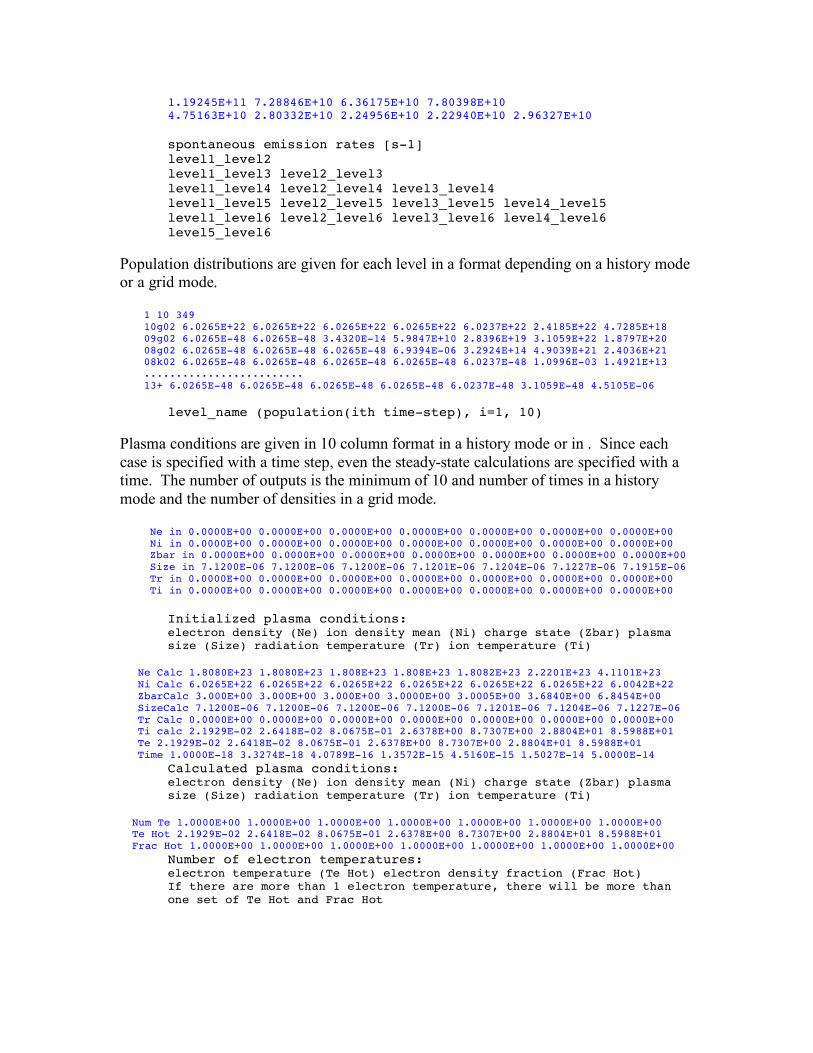
1.19245E+11 7.28846E+10 6.36175E+10 7.80398E+10 4.75163E+10 2.80332E+10 2.24956E+10 2.22940E+10 2.96327E+10 spontaneous emission rates [s-1] level1_level2 level1_level3 level2_level3 level1_level4 level2_level4 level3_level4 level1_level5 level2_level5 level3_level5 level4_level5 level1_level6 level2_level6 level3_level6 level4_level6 level5_level6
Population distributions are given for each level in a format depending on a history mode or a grid mode.
1 10 349 10g02 6.0265E+22 6.0265E+22 6.0265E+22 6.0265E+22 6.0237E+22 2.4185E+22 4.7285E+18 09g02 6.0265E-48 6.0265E-48 3.4320E-14 5.9847E+10 2.8396E+19 3.1059E+22 1.8797E+20 08g02 6.0265E-48 6.0265E-48 6.0265E-48 6.9394E-06 3.2924E+14 4.9039E+21 2.4036E+21 08k02 6.0265E-48 6.0265E-48 6.0265E-48 6.0265E-48 6.0237E-48 1.0996E-03 1.4921E+13 ......................... 13+ 6.0265E-48 6.0265E-48 6.0265E-48 6.0265E-48 6.0237E-48 3.1059E-48 4.5105E-06
level_name (population(ith time-step), i=1, 10)
Plasma conditions are given in 10 column format in a history mode or in . Since each case is specified with a time step, even the steady-state calculations are specified with a time. The number of outputs is the minimum of 10 and number of times in a history mode and the number of densities in a grid mode.
Ne in 0.0000E+00 0.0000E+00 0.0000E+00 0.0000E+00 0.0000E+00 0.0000E+00 0.0000E+00 Ni in 0.0000E+00 0.0000E+00 0.0000E+00 0.0000E+00 0.0000E+00 0.0000E+00 0.0000E+00 Zbar in 0.0000E+00 0.0000E+00 0.0000E+00 0.0000E+00 0.0000E+00 0.0000E+00 0.0000E+00 Size in 7.1200E-06 7.1200E-06 7.1200E-06 7.1201E-06 7.1204E-06 7.1227E-06 7.1915E-06 Tr in 0.0000E+00 0.0000E+00 0.0000E+00 0.0000E+00 0.0000E+00 0.0000E+00 0.0000E+00 Ti in 0.0000E+00 0.0000E+00 0.0000E+00 0.0000E+00 0.0000E+00 0.0000E+00 0.0000E+00
Initialized plasma conditions: electron density (Ne) ion density mean (Ni) charge state (Zbar) plasma size (Size) radiation temperature (Tr) ion temperature (Ti)
Ne Calc 1.8080E+23 1.8080E+23 1.808E+23 1.808E+23 1.8082E+23 2.2201E+23 4.1101E+23 Ni Calc 6.0265E+22 6.0265E+22 6.0265E+22 6.0265E+22 6.0265E+22 6.0265E+22 6.0042E+22 ZbarCalc 3.000E+00 3.000E+00 3.000E+00 3.0000E+00 3.0005E+00 3.6840E+00 6.8454E+00 SizeCalc 7.1200E-06 7.1200E-06 7.1200E-06 7.1200E-06 7.1201E-06 7.1204E-06 7.1227E-06 Tr Calc 0.0000E+00 0.0000E+00 0.0000E+00 0.0000E+00 0.0000E+00 0.0000E+00 0.0000E+00 Ti calc 2.1929E-02 2.6418E-02 8.0675E-01 2.6378E+00 8.7307E+00 2.8804E+01 8.5988E+01 Te 2.1929E-02 2.6418E-02 8.0675E-01 2.6378E+00 8.7307E+00 2.8804E+01 8.5988E+01 Time 1.0000E-18 3.3274E-18 4.0789E-16 1.3572E-15 4.5160E-15 1.5027E-14 5.0000E-14
Calculated plasma conditions: electron density (Ne) ion density mean (Ni) charge state (Zbar) plasma size (Size) radiation temperature (Tr) ion temperature (Ti)
Num Te 1.0000E+00 1.0000E+00 1.0000E+00 1.0000E+00 1.0000E+00 1.0000E+00 1.0000E+00 Te Hot 2.1929E-02 2.6418E-02 8.0675E-01 2.6378E+00 8.7307E+00 2.8804E+01 8.5988E+01 Frac Hot 1.0000E+00 1.0000E+00 1.0000E+00 1.0000E+00 1.0000E+00 1.0000E+00 1.0000E+00
Number of electron temperatures: electron temperature (Te Hot) electron density fraction (Frac Hot) If there are more than 1 electron temperature, there will be more than one set of Te Hot and Frac Hot

d) Mean Ion Charge zb.outfile.dat lists the mean charge state <zbar> and power loss rates in [erg/s/atom] from bound-bound transitions <pwrbb>, bound-free transitions <pwrbf> and free-free transitions <pwrff> at each case or each time-step. Also listed are electron temperature and density information as a function of time. If the case is stead-state, the time information will be suppressed. # case time Te Ne zbar pwrbb pwrbf pwrff pwrtt 1 1.0000E-18 2.1929E-02 1.8080E+23 3.0000E+00 0.0000E+00 1.1500E+02 4.2841E-02 1.1504E+02 2 3.3274E-18 2.6418E-02 1.8080E+23 3.0000E+00 5.8475-218 1.0477E+02 4.7156E-02 1.0482E+02 3 1.1072E-17 4.1356E-02 1.8080E+23 3.0000E+00 2.0781-217 8.3741E+01 5.9418E-02 8.3801E+01 ... ... ... ... ... ... ... ... ... ... ... ... ... ... ... ... ... ... ... ... ... ... 6 4.0789E-16 8.0675E-01 1.8080E+23 3.0000E+00 2.2608-216 1.8960E+01 2.7721E-01 1.9237E+01 7 1.3572E-15 2.6378E+00 1.8080E+23 3.0000E+00 2.0240-136 1.0485E+01 5.1456E-01 1.1000E+01 8 4.5160E-15 8.7307E+00 1.8082E+23 3.0005E+00 1.2893E-42 5.7659E+00 9.6444E-01 6.7304E+00 9 1.5027E-14 2.8804E+01 2.2201E+23 3.6840E+00 2.5783E-10 5.8661E+00 3.4029E+00 9.2690E+00 10 5.0000E-14 8.5988E+01 4.1101E+23 6.8454E+00 3.5079E+01 3.1323E+01 3.6930E+01 1.033E+02
e) Ion Stage Distributions pp.outfile.dat lists the fraction of each ionization stage at each time step (# case time for history mode or steady for grid mode) from the neutral ionization stage (0) to the bare nuclei (13, atomic number). Numbers less than 1.e-30 should be considered as zero. # case steady Te Ne 0 ... 10 11 12 13 1 ***** 1.00E+03 1.00E+21 2.85E-48 ... 1.73E-04 4.08E-02 4.70E-01 4.89E-01 2 ***** 1.00E+03 1.00E+22 5.56E-42 ... 4.64E-04 3.20E-02 3.95E-01 5.72E-01 3 ***** 1.20E+03 1.00E+21 1.58E-49 ... 6.50E-05 2.04E-02 3.49E-01 6.31E-01 4 ***** 1.20E+03 1.00E+22 1.54E-43 ... 2.22E-04 1.57E-02 2.91E-01 6.93E-01
(2) FLYSPEC There are two output files in a table right next to the plot, Spectrum and Lines. The spectrum file has two columns of photon energy [eV] and intensity [ergs/cm2/s/Hz/srad] and the lines file has the list of information of dominant transitions. The header information includes Iso Energy Intensity Emissivity Tau Arates Width LowLevel UpLevel LowLevelName UpLevelName. The Energy refers to the line-center energy, Emissivity, Tau (optical depth) Arates refer to the values at the line-center of the transition. The Width is the greater value of STA width and UTA width of a STA transition. LowLevel UpLevel refer to the level index of the lower and upper levels of the transition and LowLevelName UpLevelName to the level names of FLYCHK code. If the STA lines are used, they refer to the orbitals of initial and final states. If NIST ASD lines are used, the same level notation as that of NIST ASD is used to give transition information. The Intensity refers to the line-center intensity of the transition if the line is isolated, in other words, there is no emissivity or opacity from other lines at the energy. Therefore the Intensity is different from the total intensity at the line-center energy since the total intensity includes the contribution from all bound-bound and bound-free, free-free transitions.

V) EXAMPLES Examples of input runfiles which list a series of input commands are presented as well as necessary data files such as history files, radiation field input data files or non-Maxwellian electron energy distribution data files. The same examples are shown at the EXAMPLES section at the website (http://nlte.nist.gov/FLY/EXAMPLE.html) along with screen shot of the input webpage.
A. Steady-state calculations on grid input Description Runfile Additional Info or Input Files
a grid of given electron densities (ne) and electron temperature (te)
z 13 initial ss evolve ss history grid ne ne 1e20 1e24 10 te 50 300 50 end
Case showing grid input using electron density
A grid of given ion densities (nt) and electron temperature (te)
z 13 initial ss evolve ss history grid nt nt 6e18 6e22 10 te 50 300 50 end
Case showing grid input using from Case 1 differences using ion density
a grid of given mass densities (rho) and electron temperature (te)
z 13 initial ss evolve ss history grid rho rho 0.027 2.7 10 te 50 300 50 end
Case showing grid input using from Case 1 differences using mass density
2nd Maxwellian hot electrons of 100 keV and 1 % of the total electron density
z 29 initial ss evolve ss fhot fixed 0.01 1.e5 history grid ne ne 1e20 1e24 10 te 100 1000 100 end
Case showing the grid data and effects of a hot electron component
blackbody radiation of 100 eV and 1 % dilution factor
z 29 initial ss evolve ss tr 100. dilution 0.01 history grid ne ne 1e20 1e22 10 te 100 1000 100 end
Case showing the grid data and effects of a dilute balckbody radiation field
optically thick plasmas of 1 microns
z 29 initial ss evolve ss opacity size 0.0001 history grid nt nt 6e18 6e22 10 te 100 1000 100 end
Case showing the grid data and effects of optical depth
mixture option: krypton embedded in D2, He (Z=2)
z 36 initial ss evolve ss mixture 2.8 0.99961 5. history grid rho
ICF imploded core conditions
Case shows use of the mixture option

rho 0.2 2. 10. te 2000 5000 1000 end
monoenergetic electron beam Please note that each case, though stead-state, has the corresonding time used with fe(E) (EEDF: electron energy distribution function) inputs
z 79 initial ss evolve ss fe file fedata.d history grid ne ne 1e5 1e12 1e7 te 10. 20. 10. end
EBIT plasma case
fedata.d (# of times # of energy grid pts) 2 3 (energy pts) 4.49E+03 4.5E+03 4.51E+03 (time 1, # of beam e-) 0.0E+00 1.0E+11 (3 time 1 fe pts) 1.0E-20 1.49071E-03 1.0E-20 (time 2, # of beam e-) 1.0E-09 1.0E+11 (3 time 2 fe pts) 1.0E-20 1.49071E-03 1.0E-20
user-defined radiation field Please note that each case has the corresonding time used with radiation field input
z 12 initial ss evolve ss tr trifle xfel.d history grid ne ne 1e21 1e21 1.1 te 50. 100. 50. end
XFEL-driven plasma case
xfel.d (use only numbers written) (# of times # of photon grid pts.) 2 2 (photon energy pts) 3.09695E+03 3.10305E+00 (time 1, radiation temperature) 0.0E+00 0.0E+00 (radiation field at time 1) 9.3018e2 9.3018e2 (time 2,radiation temperature) 1.0E-12 0.0E+00 (radiation field at time 1) 9.3018e15 9.3018e15
B. Steady-state calculations on history input Description Runfile Additional Info or Input Files
given ne and te that can not be on a grid
z 13 initial ss evolve ss history alne ne end
alne time ne te 0.e-12 1.e20 50 1.e-12 1.e20 100 2.e-12 1.e20 500 3.e-12 1.e21 50 4.e-12 1.e21 100 5.e-12 1.e21 500
given nt and te that can not be on a grid
z 13 initial ss evolve ss history alnt nt end
alnt time nt te 0.e-12 6.e18 50 1.e-12 6.e18 100 2.e-12 6.e18 500 3.e-12 6.e20 50 4.e-12 6.e20 100 5.e-12 6.e20 500
both ne and nt given
z 13 initial ss evolve ss history alnent ne nt end
alnent time ne nt te 0.e-12 1.e20 6.e18 50 1.e-12 1.e20 6.e18 100 2.e-12 1.e20 6.e18 500 3.e-12 1.e22 6.e20 50 4.e-12 1.e22 6.e20 100 5.e-12 1.e22 6.e20 500
both ne and rho given
z 13 initial ss evolve ss
alnerho time ne rho te 0.e-12 1.e20 0.027 50

history alnerho ne rho end
1.e-12 1.e20 0.027 100 2.e-12 1.e20 0.027 500 3.e-12 1.e22 0.270 50 4.e-12 1.e22 0.270 100 5.e-12 1.e22 0.270 500
opacity effect from the history file hot e- distribution of 1% and 1 MeV
z 29 initial ss evolve ss opacity file fhot file history cuhotop ne end
cuhotop time ne te size fhot thot 0.e-12 1.e23 50 1.e-4 0.01 1.e6 1.e-12 1.e23 100 1.e-4 0.01 1.e6 2.e-12 1.e23 500 1.e-4 0.01 1.e6 3.e-12 1.e23 1e3 1.e-4 0.01 1.e6
opacity effect fixed by size input hot e- distribution of 1% and 1 MeV
z 29 initial ss evolve ss opacity size 1.e-4 fhot fixed 0.01 1.e6 history cune ne end
cune time ne te 0.e-12 1.e23 50 1.e-12 1.e23 100 2.e-12 1.e23 500 3.e-12 1.e23 1e3
blackbody radiation at 100 eV and dilution factors
z 29 initial ss evolve ss tr file history cutr ne end
cutr time ne te tr dilution 0.e-12 1.e22 100 100 1.0 1.e-12 1.e22 100 100 0.1 2.e-12 1.e22 100 100 0.01 3.e-12 1.e22 100 100 0.001
user-defined radiation field
z 12 initial ss evolve ss tr trifle xfel.d history mgne ne end
mgne time ne te 0.e-12 1.e21 50 1.e-12 1.e21 100 xfel.d 2 2 3.09695E+03 3.10305E+00 0.0E+00 0.0E+00 9.3018e2 9.3018e2 1.0E-12 0.0E+00 9.3018e15 9.3018e15
C. Time-dependent calculations on history input Description Runfile Additional Info or Input Files
initially LTE state time-dependent rho and te opacity effect time steps in history file are used as output time steps
z 13 initial lte evolve td opacity file history alhydro rho end
history file: alhydro time te rho size 0.00E+00 0.02 2.70 7.12e-06 1.04E-14 20.08 2.70 7.121e-06 2.15E-14 41.01 2.70 7.125e-06 3.05E-14 56.26 2.70 7.134e-06 4.25E-14 75.74 2.69 7.161e-06 5.38E-14 91.18 2.69 7.207e-06
initial populations using steady-state calculations opacity effect time steps in history file are used as output time steps
z 13 initial ss evolve td opacity file history alhydro rho end
history file: alhydro time te rho size 0.00E+00 0.02 2.70 7.12e-06 1.04E-14 20.08 2.70 7.121e-06 2.15E-14 41.01 2.70 7.125e-06 3.05E-14 56.26 2.70 7.134e-06 4.25E-14 75.74 2.69 7.161e-06 5.38E-14 91.18 2.69 7.207e-06
initial populations specified in a file
z 13 initial file algs evolve td opacity file
history file: alhydro Population file: algs (use only the numbers)

For information on the name of levels in the model, please refer to output description
history alhydro rho end
(name of level, fraction) 13g03 1.d0
even time step from 0 to 500 fs # of outputs is 6 in this case. Note that the maximum # of time steps is 500
z 13 initial lte evolve td opacity file history alhydro rho time 0 5.e-14 6 end
history file: alhydro Modify the time-steps for output
logarithmic time step from 1 atto-seconds to 500 fs # of output is 10 in this case
z 13 initial lte evolve td opacity file history alhydro rho time log 1.e-18 5.e-14 10 end
history file: alhydro Modify the time-steps for output There are other options such as pump, which allows logarithmic time steps first and linear time steps later, or hybrid , which allows linear steps first and log steps later.
Recombining plasmas initially bare nuclei given nt and te
z 6 initial file cbare evolve td history crecom nt time 0. 0.2 41 end
Shows initial populations set with a file and a plasma that is cooling as it recombines crecom time te nt 0.0E-00 300. 1.0E+13 5.0E-04 299. 1.0E+13 4.0E-02 281. 1.0E+13 1.0E-01 142. 1.0E+13 1.5E-01 41.0 1.0E+13 2.0E-01 18.0 1.0E+13 cbare 6+ 1.0E+13
initially neutral ground state given ne, nt and te 2nd Maxwellian hot electrons of 100 keV and 1 % of the total electron density log first (10 steps) and linear later (100 steps) output time steps
z 29 initial file cuneutral evolve td fhot fixed 0.01 1.e5 history cuionz ne nt time pump 1.e-18 1.e-13 5.e-12 10 100 end
Shows an ionizing plasma starting from the neutral species specified by a file, with the main electron temperature set by the history file and a hot electron component set by the "fhot" option. cuionz time te ne nt 0.00E-00 1000. 1.E+23 8.E+22 1.00E-06 1000. 1.E+23 8.E+22 cuneutral 29g04 8.E+22
REFERECES 1 D. Mihalas, Stellar Atmospheres, 2nd Ed. San Francisco; W.H. Freeman, 1978
2 R. W. P. McWhirter, Spectral intensities, Plasma Diagnostic Techniques, edited by R. H. Huddlestone and S. L. Leonard, p.206 (1965) New York , Academic Press
3 T. D. Shepard et al., Review of Scientific Instruments, v.66, p.749 (1995); C. J. Keane et al., Journal of Quantitative Spectroscopy and Radiative Transfer, 51, 147 (1993); J. P. Matte et al., Laser and Particle Beams, 12, 455 (1994)

4 A. Rousse et al., Journal of Physics B: Atomic, Molecular and Optical Physics, 27, L697 (1994); T. Kawamura et al., PHYSICAL REVIEW E 66, 016402 (2002)
5 R. W. John, Laser and Particle Beams,13, 365 (1995)
6 Lee RW, Larsen JT. A time-dependent model for plasma spectroscopy of K-shell emitters, J Quant Spectrosc Radiat Transfer. 1996;56:535 7 P. Wang et al., Review of Scientific Instruments, 68, 1107 (1997)
8 B. G. Wilson et al., in Atomic Processes in Plasmas, edited by E. S. Maramar and J. L. Terry (AIP, New York, 1991), p. 189. 9 Y. Maron et al., Physical Review A, 39, 5856 (1989); Y. Maron et al., Physical Review A, 40, 3240 (1989); M. E. Foord, Y. Maron and E. Sarid, Journal of Applied Physics, 68, 5016 (1990)
10 J. E. Bailey, H. K. Chung, A. L. Carlson, D. Cohen, D. J. Johnson, P. Lake, J. J. MacFarlane, P. Wang, and D. R. Welch, Phys. Rev. Lett. 82, 739 - 742 (1999) 11 J. Abdallah Jr. et al., Journal of Quantitative Spectroscopy and Radiative Transfer, 50, 91 (1993)
12 R. C. Isler et al., Physics of Plasmas, 4, 355 (1996); K. B. Fournier et al., Physical Review E, 53, 1084 (1996)
13 M. Pockl et al., Journal of Applied Phyics, 76, 733 (1994); M. E. Yaakoubi and P. Ranson, Journal of Physics D: Applied Physics, 26, 937, (1993)
14 P. V. Storm and M. A. Cappelli, Journal of Quantitative Spectroscopy and Radiative Transfer, 56, 901 (1996)
15 C. Barue, Journal of Applied Physics, 76, 2662 (1994)
16 J. C. Raymond and N. S. Brickhouse, Astrophysics and Space Science, 237, 321 (1996); N. S. Brickhouse et al., The Astrophysical Journal Supplement Series, 97, 551 (1995)
17 Lee RW, Nash JK, Ralchenko Y, Review of the NLTE kinetics code workshop, J. Quant Spectrosc Radiat Transfer. 1997;58:737 18 C. Bowen, R.W. Lee and Yu. Ralchenko, Journal of Quantitative Spectroscopy and Radiative Transfer, 99, (2006) 102-119 19 J.G. Rubiano, R. Floridoa, C. Bowen, R.W. Lee and Yu. Ralchenko, High Energy Density Physics, 3, (2007) 225-232 20 D. R. Inglis and E. Teller, The Astrophysical Journal, 90, 439 (1939); D. G. Hummer and D. Mihalas, The Astrophysical Journal, 331, 794 (1988)
21 H. R. Griem, Plasma Spectroscopy, (1964) McGraw-Hill
22 J. J. MacFarlane, UWFDM-937, Univ. of Wisconsin Fusion Technology Institute Report (1993)
23 J. P. Apruzese, Journal of Quantitative Spectroscopy and Radiative Transfer, 23, 479 (1980); J. P. Apruzese, Journal of Quantitative Spectroscopy and Radiative Transfer, 25, 419 (1981); J. P. Apruzese, Journal of Quantitative Spectroscopy and Radiative Transfer, 33, 71 (1985); J. P. Apruzese, Journal of Quantitative Spectroscopy and Radiative Transfer, 34, 447 (1985)
24 D. Robinson and P. D. Lenn, Applied Optics, 6, 983 (1967)
25 C. A. Back et al., 10th Topical Conference on Atmoic Processes in Plasmas, edited by A. L. Osterheld and W. H. Goldstein, 123, (1996) San Francisco

26 W. L. Wiese, Plasma Diagnostic Techniques, edited by R. H. Huddlestone and S. L. Leonard 265 (1965) New York, Academic Press
27 G. B. Rybicki and A. P. Lightman, Radiative Processes in Astrophysics (1981) Wiley
28 H.K. Chung, D.H. Cohen, J.J. MacFarlane, J.E. Bailey, P. Wang and G.A. Moses, Journal of Quantitative Spectroscopy and Radiative Transfer 65, (2000), 135-149 29 Kelly RL, Journal of Physical and Chemical Reference Data, Supplement. 1987;16:1 30 Scofield JH. Energies Of Hydrogen- and Helium-Like Ions For Z From 6 To 54. Internal Document, UCID-16848, Lawrence Livermore National Laboratory, 1975; Saloman EB, Hubbell JH, Scofield JH, X-ray attenuation cross sections for energies 100 eV to 100 keV and elements Z=1 to Z=92. Atomic Data & Nuclear Data Tables, 1988:38:1 31 Chenais-Popovics C, Malka V, Gauthier JC, Gary S, Peyrusse O, Rabec-Le Gloahec M, Matsushima I, Bauche-Arnoult C, Bachelier A, Bauche J. X-ray emission of a xenon gas jet plasma diagnosed with Thomson scattering Phys. Rev. E 2002;65:046418 32 Savin DW, Bartsch T, Chen MH, Kahn SM,. Liedahl DA, Linkemann J, Müller A, Schippers S, Schmitt M, Schwalm D, and Wolf A, Dielectronic Recombination in Photoionized Gas: The Importance of Fine-structure Core Excitations. Ap. J. 1997;489:L115 33 Huang KN, Aoyagi M, Chen MH, Crasemann B. Neutral-atom electron binding energies from relaxed-orbital relativistic Hartree-Fock-Slater calculations. At. Dat. Nuclear. Dat. Tables 1976;18:243 34 Bar-Shalom A, Klapisch M, Oreg J. HULLAC, an integrated computer package for atomic processes in plasmas. J. Quant Spectrosc Radiat Transfer. 2001;71:169
35 Lee RW, Larsen JT. A time-dependent model for plasma spectroscopy of K-shell emitters, J Quant Spectrosc Radiat Transfer. 1996;56:535 36 Scofield JH. Phys. Rev. A. 1989;40:3054 37 Kramers H. Philos Mag. 1923:46:836 38 Oxenius J. Kinetic Theory of Particles and Photons, Berlin; Springer-Verlag, 1986. p. 21-65
39 Van Regemorter H. Ap. J. 1962;136:906 40 Mewe R. Interpolation formulae for the electron impact excitation of ions in the H-, He-, Li, and Ne-sequences. Astron. Astrophys. 1972;20:215 41 Golden LB, Sampson DH, Electron-impact cross-sections and rates for nl→n’l’ transitions in hydrogenic ions and hydrogen. Astrophys. J. 1971;170:181 42 Lotz W, Z. Phys. 1968;216:241, Lotz W, Z. Phys. 1969;220:266 43 Burgess A, Chidichimo MC. Electron impact ionization of complex ions. Mon. Not. R. astr. Soc. 1983;203:1269
44 Golden LB, Sampson DH, Electron-impact cross-sections and rates for nl→n’l’ transitions in hydrogenic ions and hydrogen. Astrophys. J. 1971;170:181 45 Shoub EC. Departures of the electron energy distribution from a Maxwellian in hydrogen. I. Formulation and solution of the electron kinetic equation. Ap J. Suppl. Ser. 1977;34:259 46 Sobelman II, Vainshtein LA, Yukov EA. Excitation of atoms and broadening of spectra lines. 2nd Ed. Berlin; Springer, 1995. p. 120-124 47 Van Regemorter H. Ap. J. 1962;136:906

48 Chen MH, Laiman E, Casemann B, Aoyagi M, Mark H. Relativistic L-shell Auger and Coster-Kronig rates and fluorescence yields. Phys. Rev. A. 1979;19;2253 49 Inglis DR, Teller E. Ionic depression of series limits in one-electron spectra. Astrophys. J. 1939;90:439 50 Stewart JC, Pyatt KD. Lowering of ionization potentials in plasmas. Astrophys. J. 1966;144:1203 51 R. M. More, in Applied Atomic Collision Physics, 2, Academic Press, New York (1982) 52 Mihalas D. Stellar Atmospheres, 2nd Ed. San Francisco; W.H. Freeman, 1978. Ch. 4, Ch. 9 and Ch. 11 53 A. C. Hindmarsh, L. J. Sloan and P. F. Dubois, Lawrence Livermore Laboratory Report, UCID-30137, revision 1, December 1978 54 D. Mihalas, Stellar Atmospheres, second edition chapter 11 (W.H. Freeman, San Francisco) 1978 55 A. C. Hindmarsh in Scientific Computing, edited by R. S. Steplemen et al. p. 55 (North-Holland, Amsterdam) 1983: for a current source of information on LSODE see the internet address: http://ute.usi.utah.edu/software/math/lsode.html 56. Drayson, J.Q.S.R.T. 16, 611 (1976) 57 Karzas WJ, Latter R. Electron radiative transitions in a coulomb field. Ap. J. Suppl. 1961;55:167 58 A. Bar-Shalom, J. Oreg, W. H. Goldstein, D. Shvarts, A. Zigler, Phys. Rev. A 40, 3183 - 3193 (1989)