manual for using jmp with principles & methods of

Manual for using JMP with Principles & Methods of Statistical Analysis

Having students create formulas in JMP software program is an excellent way for them to understand how the computational techniques we frequently use work. We have created a number of step-by-step instructional guides to help you in this regard. Each instructional section is set up to guide your students – step-by-step – through these data analytic techniques with the data sets discussed in the textbook. By recreating the results presented in the textbook through the use of JMP, students will broaden their understanding of the underlying techniques we use to within our field.

Contents

Chapter Procedures . Chapter 2. Histograms 3 Quantile Plots 5 Stem-and-Leaf Displays 7 Box Plots 9 Normal Quantile Plots 10 Kolmogorov-Smirnov-Lilliefors Goodness of Fit Test 12 Shapiro-Wilk W Test 12 Chapter 3. Generating Populations 14 Adding, Subtracting, Multiplying, Dividing by Constants, z-scores 14 Adding, Subtracting Scores from Two Distributions 18 Central limit theorem 20 Chapter 4. Demonstrating confidence Intervals for the Mean of a Normal Distribution 24 Chapter 5. Trimmed Means, MAD (Median of Absolute Deviations from the Median), One-step M-estimators 26 Winsorized Means, Winsorized Variances 28 Bootstrap Estimators 30 Chapter 7. Student’s t, Welsh-Satterthwaite t 32 Empirical Quantitle-Quantile Plots 34 Mean Diamonds 36

Standardized effect sizes 38 Chapter 8. Binomial Test 40 Chi Square Goodness of Fit Test 42 Chapter 9. Approximate randomization test for difference between two groups 44 Chapter 10. Approximate randomization test for correlation between two variables 47 Bivariate Normal Distribution Hypothesis Tests 50 Bivariate Normal Distribution Confidence Intervals 50 Bootstrap Confidence Intervals for Population Correlations 50 Spearman r, Kendall’s Tau 53 Chi Square test for Association 55 Chapter 11. Linear Regression F and t tests 57 Chapter 12. Checking Assumptions in Regression 59

2

Non-linear Regression and Lack of Fit tests 61 Chapter 13. Point biserial r 65 Chapter 14. One-way ANOVA 67 Relational Effect Size Measures 68 Approximate Randomization Test for ANOVA 70 Two-way ANOVA 73 Chapter 15. Simple Slopes of Continuous x Continuous 75 Simple Slopes of Categorical x Continuous 79

3

The dataset titled “JMP Data File Barlett 2015” is used for the following examples UNLESS otherwise noted Chapter 2 – Examining Our Data

I. Histograms Objective: Create a histogram of the variable State Hostility Scale score (SHS score)

1. From data table, click Analyze then Distribution. 2. Select “SHS score” and click/drag to the Y,Columns, then click OK.

3. Click on the second Red Triangle next to SHS score; click on Display Options; click on Horizontal Layout.

4

4. Result is the following histogram with descriptive statistics:

5

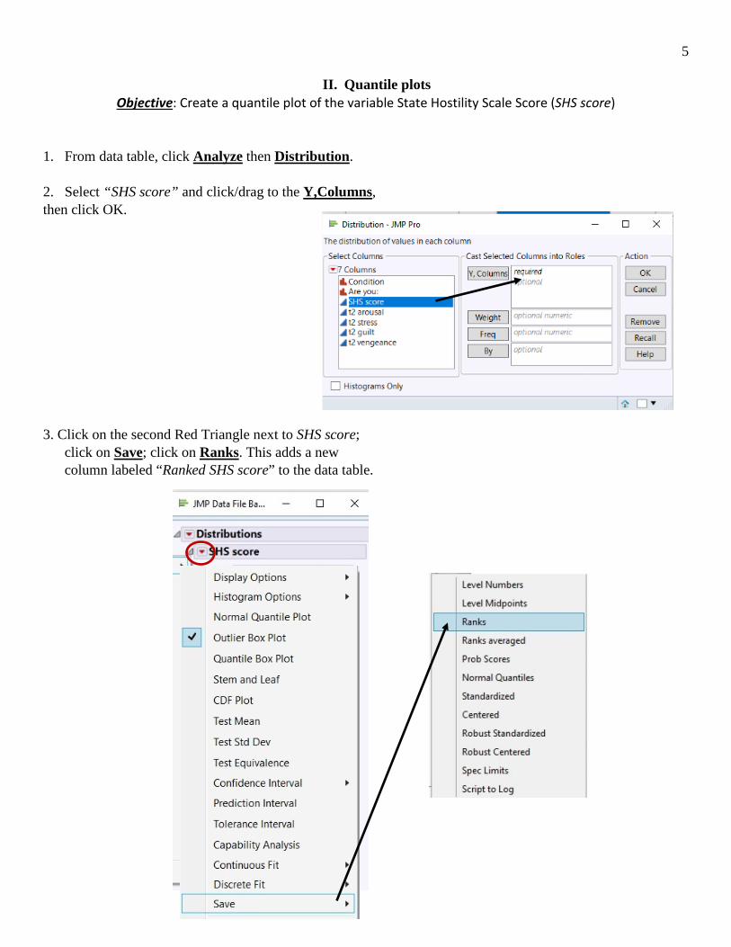
II. Quantile plots Objective: Create a quantile plot of the variable State Hostility Scale Score (SHS score)


3. Click on the second Red Triangle next to SHS score; click on Save; click on Ranks. This adds a new column labeled “Ranked SHS score” to the data table.

6

4. From the data table with the new column, click Analyze, then click Fit Y by X. Click/drag SHS score to the

Y,Response box; click/drag Ranked SHS score to the X, Factor box. Click OK. 6. The result is the following quantile plot:

7

III. Stem-and-leaf displays

Objective: Create a stem-and-leaf display of the variable State Hostility Scale Score (SHS score)


3.Click on the second Red Triangle next to SHS score; click on Steam and Leaf.

8

4. The result is the following stem-and-leaf display:

9

IV. Box Plots Objective: Create a box-plot of the variable State Hostility Scale Score (SHS score) by two levels of the

condition of Message (Nice, Insult)

1. From data table, click Graph, then Graph Builder. 2. Select “Total fat g” and click/drag to the x-axis. Then select Box Plot 3. The result is the following box plot:

10

V. V. Normal Quantile Plots (Q-Q)

Objective: Create a normal quantile plot of the variable State Hostility Scale Score (SHS score)


3.Click on the second Red Triangle next to SHS score; click on Normal Quantile Plot.

11

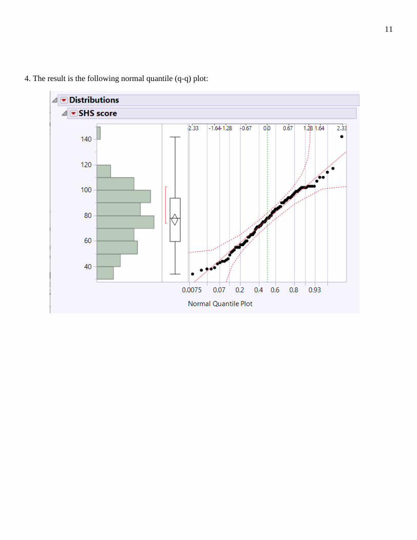
4. The result is the following normal quantile (q-q) plot:

12

VI. Goodness of Fit Test to a Normal Distribution Objective: Conduct a goodness-of-fit test on the variable State Hostility Scale Score (SHS score)

**Note: When n < 2000, the result is the Shapiro-Wilk Test. When n > 2000, the result is the Kolmogorov-Smirnov Test. In this example, n = 114, so the Shapiro-Wilk Test is shown.


3. Click on the second Red Triangle next to SHS score; Click on Continuous Fit, then on Normal

13

4. Click on the Red Triangle next to Fitted Normal; then click on Goodness of Fit 5. The result is the following output (is p < .05?)

14

Chapter 3: Properties of Distributions I. Using the “Formula” Function (adding, subtracting, multiplying, dividing by constants)

Objective: Adding 10 to the t2 vengeance variable **Note that this example adds a constant to a variable. The same steps can be used to subtract, multiply, and divide constants to variables as well. **

1. Add a new column by clicking on Cols, then New Columns. Name the new column/variable (e.g., NEW t2 vengeance). Click OK. Then right-click on NEW t2 vengeance, and click on Formula. 2. Click on the variable you are using to create the new variable (e.g., t2 vengeance). You should see it entered into the Formula screen/box. Then click “+” at the top, then enter “10”. Click OK.

15

3. The new variable “NEW t2 vengeance” should fill in, adding 10 to each row of t2 vengeance.

16

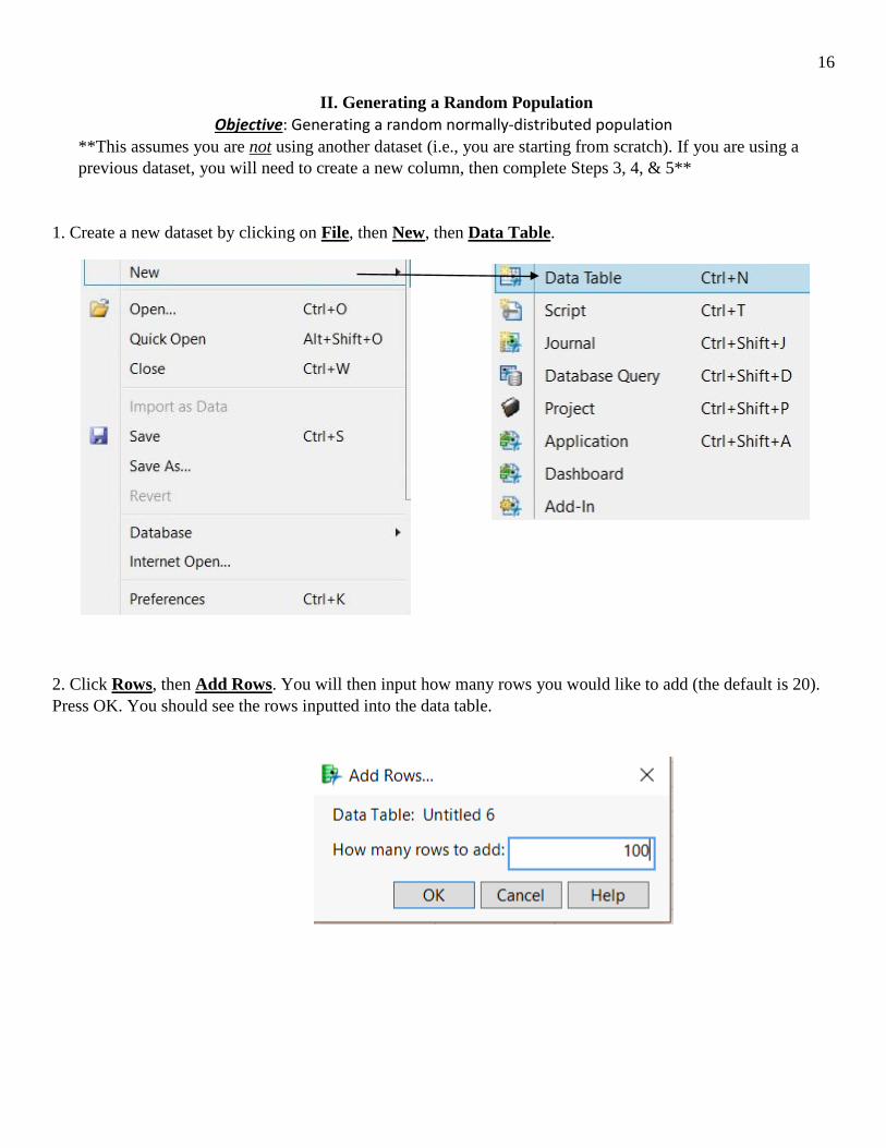
II. Generating a Random Population Objective: Generating a random normally-distributed population

**This assumes you are not using another dataset (i.e., you are starting from scratch). If you are using a previous dataset, you will need to create a new column, then complete Steps 3, 4, & 5**

1. Create a new dataset by clicking on File, then New, then Data Table. 2. Click Rows, then Add Rows. You will then input how many rows you would like to add (the default is 20). Press OK. You should see the rows inputted into the data table.

17

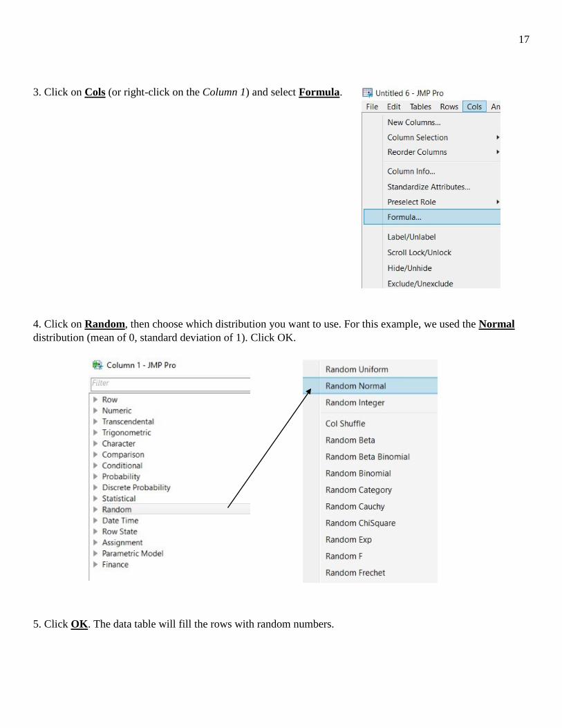
3. Click on Cols (or right-click on the Column 1) and select Formula. 4. Click on Random, then choose which distribution you want to use. For this example, we used the Normal distribution (mean of 0, standard deviation of 1). Click OK. 5. Click OK. The data table will fill the rows with random numbers.

18

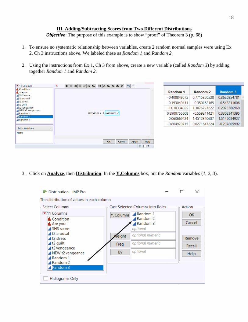
III. Adding/Subtracting Scores from Two Different Distributions Objective: The purpose of this example is to show “proof” of Theorem 3 (p. 68)

1. To ensure no systematic relationship between variables, create 2 random normal samples were using Ex

2, Ch 3 instructions above. We labeled these as Random 1 and Random 2.

2. Using the instructions from Ex 1, Ch 3 from above, create a new variable (called Random 3) by adding together Random 1 and Random 2.

3. Click on Analyze, then Distribution. In the Y,Columns box, put the Random variables (1, 2, 3).

19

4. Click OK. Click on the Red Triangle for each Summary Statistics box, click Customize Summary Statistics, select Variance, and click OK (you will need to do this for each distribution/variable).

5. You should have results similar to below. To exemplify Theorem 3, note that the first two means (Random 1 and 2) add to equal Random 3’s mean.

20

IV. Central Limit Theorem

Objective: The purpose of this example is to show “proof” of Theorem 7 (p. 77)

1. At the JMP Home Window, click Help, then Sample Data. (NOT Sample Data Library). Click on Simulations, under Teaching Resources, then click on Central Limit Theorem.

2. A new data table will be displayed. Click Rows, then Add Rows. Input 2,000 rows and click OK.

21

3. The data table should populate. Click Analyze, then Distribution. Click/drag each column over to the Y,Columns Box. Click OK. 4. Click on the Red Triangle by Distribution, and select Stack.

22

5. For each histogram, right-click the x-axis, click on Axis Settings. Set the minimum to 0 and maximum to 1. 6. Click the Red Triangle for each Distribution, click on Continuous Fit, then click on Normal.

23

7. Click on the Red Triangle on the Fitted Normal output, then click on Goodness of Fit (is p < .05?) 8. Refer to the Shapiro-Wilk/Kolmogorov-Smirnov Test results – is p < .05?

24

Chapter 4: Estimating Parameters of Populations from Sample Data I. Confidence Intervals for the Mean of a Normal Distribution

Objective: To produce a sample confidence interval 1. At the JMP Home Window, click Help, then Sample Data. (NOT Sample Data Library). Click on Simulations, under Teaching Resources, then click on Teaching Scripts. Under that, click on Interactive Teaching Modules, then click on Confidence Interval for the Population Mean. 2. Under Population Characteristics: Select Normal for Population Shape Enter Population Mean (e.g., 100) & Standard Deviation (e.g., 10) Enter name of variable (e.g., IQ) 3. Under Demo Characteristics: Enter Sample Size (e.g., 75), Number of Samples (e.g., 100), & Confidence Level (e.g., .95) Select “Yes” for known Population Std Dev

25

Select your preference for Animate Illustration 4. Click Draw Additional Samples 5. The results will be displayed, including the Upper and Lower bounds of the Confidence Interval:

26

Chapter 5: Resistant Estimators of Parameters I. Trimmed Mean, MAD (Median of the Absolute Deviations from the median), M-Estimator (Robust Mean) Objective: To produce the trimmed mean, MAD, and Robust Mean for State Hostility score (SHS score)


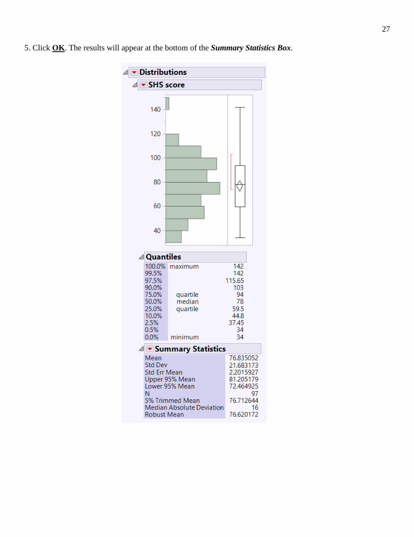
3. Click on the Red Triangle by Summary Statistics, Select Customize Summary Statistics 4. Select the following resistant estimators: Trimmed Mean, Median Absolute Deviation, Robust Mean. *At the bottom, enter the percent for the Trimmed Mean (default is 5%).

27

5. Click OK. The results will appear at the bottom of the Summary Statistics Box.

28

II. Winsorized Means & Variances

Objective: To produce the winsorized mean and variance for State Hostility score (SHS score)

**This requires the Extended Summary Statistics Add-In, which can be downloaded from https://community.jmp.com/t5/JMP-Add-Ins/tkb-p/add-ins **

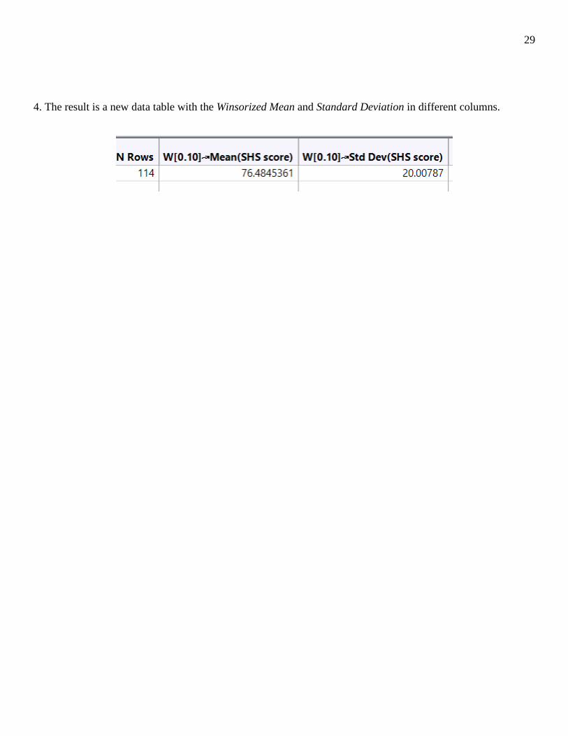
1. On the top menu, click on Add-Ins, then click on the appropriate add-in (i.e., Extended Summary Statistics) 2. Select Winsorize from the Trim/Winsorize drop-down menu. Input what proportion you would like to winsorize (the default is .10). 3. Highlight SHS score, then click Mean and Std Dev from the Statistics drop-down menu. Click OK.

https://community.jmp.com/t5/JMP-Add-Ins/tkb-p/add-ins

29

4. The result is a new data table with the Winsorized Mean and Standard Deviation in different columns.

30

III. Bootstrap Estimators Objective: To compare the State Hostility score (SHS score) between the two levels of Message (Insult, Nice)


3. Right-click on Mean located in the Summary Statistics section. Select Bootstrap. 4. In the menu that appears, enter the number of Bootstrap samples you want (default is 2500). Be sure to leave the two boxes checked, and click OK.

31

5. A new data table is generated, containing a column with each bootstrap sample (labeled BootID), where the first row contains the original estimates (hence BootID of 0). 6. In this new data table, click Analyze, then Distribution. Select the estimator interested in (i.e., Mean) and move to the Y,Columns box. Click OK. 7. The result contains bootstrap confidence intervals on the bottom.

32

Chapter 7: Independent Groups t-Test I. Student’s t-test & Welch-Satterthwaite t-test

Objective: To compare the State Hostility score (SHS score) between the two levels of Message (Insult, Nice) 1. Click Analyze, then select Fit Y by X. 2. Select the predictor variable (i.e., Condition) and click/drag to the X,Factor box. Select the outcome variable (i.e., SHS score) and click/drag to the Y,Response box. Click OK. 3. A. For student’s t-test, click on the Red Triangle, then select Means/ANOVA/Pooled t

33

The value of student’s t is the t Ratio located in the t Test section. B. For Welch-Satterthwaite t, click on the Red Triangle, then select t test. The value of student’s t is the t Ratio located in the t Test section at the bottom.

34

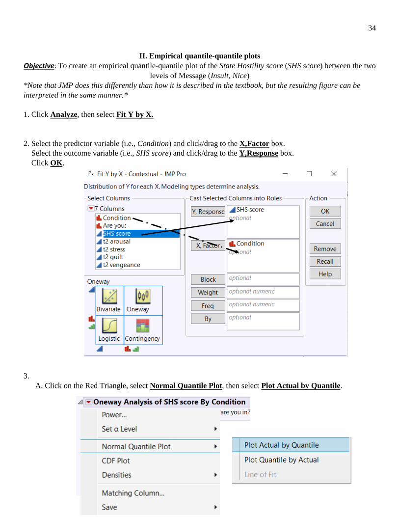
II. Empirical quantile-quantile plots

Objective: To create an empirical quantile-quantile plot of the State Hostility score (SHS score) between the two levels of Message (Insult, Nice)

*Note that JMP does this differently than how it is described in the textbook, but the resulting figure can be interpreted in the same manner.* 1. Click Analyze, then select Fit Y by X. 2. Select the predictor variable (i.e., Condition) and click/drag to the X,Factor box. Select the outcome variable (i.e., SHS score) and click/drag to the Y,Response box. Click OK. 3. A. Click on the Red Triangle, select Normal Quantile Plot, then select Plot Actual by Quantile.

35

4. The result is the following graph. When the lines are parallel, the treatment is additive with the treatment effect indicated by the difference between the lines. When the lines diverge, the treatment is multiplicative. Also note that this works with both equal and unequal samples sizes.

36

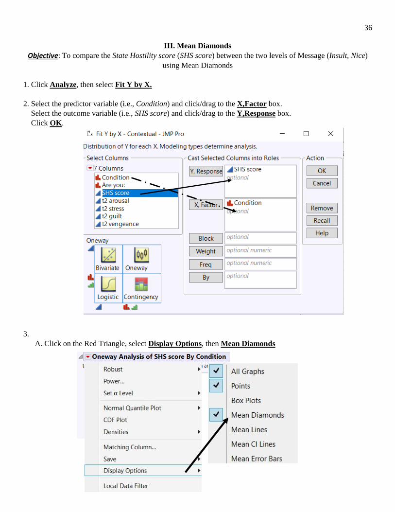
III. Mean Diamonds Objective: To compare the State Hostility score (SHS score) between the two levels of Message (Insult, Nice)

using Mean Diamonds

1. Click Analyze, then select Fit Y by X. 2. Select the predictor variable (i.e., Condition) and click/drag to the X,Factor box. Select the outcome variable (i.e., SHS score) and click/drag to the Y,Response box. Click OK. 3. A. Click on the Red Triangle, select Display Options, then Mean Diamonds

37

4. The mean diamonds will appear in the graph.

38

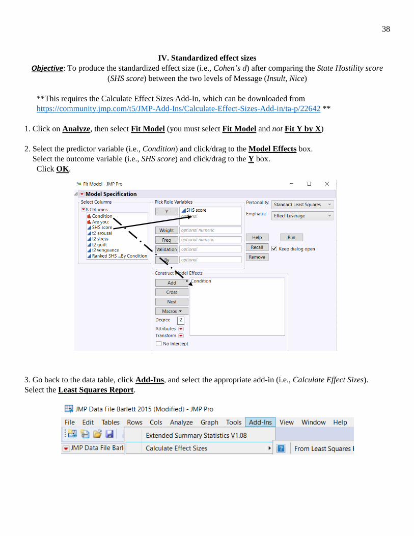
IV. Standardized effect sizes

Objective: To produce the standardized effect size (i.e., Cohen’s d) after comparing the State Hostility score (SHS score) between the two levels of Message (Insult, Nice)

**This requires the Calculate Effect Sizes Add-In, which can be downloaded from https://community.jmp.com/t5/JMP-Add-Ins/Calculate-Effect-Sizes-Add-in/ta-p/22642 **

1. Click on Analyze, then select Fit Model (you must select Fit Model and not Fit Y by X) 2. Select the predictor variable (i.e., Condition) and click/drag to the Model Effects box. Select the outcome variable (i.e., SHS score) and click/drag to the Y box. Click OK. 3. Go back to the data table, click Add-Ins, and select the appropriate add-in (i.e., Calculate Effect Sizes). Select the Least Squares Report.

https://community.jmp.com/t5/JMP-Add-Ins/Calculate-Effect-Sizes-Add-in/ta-p/22642

39

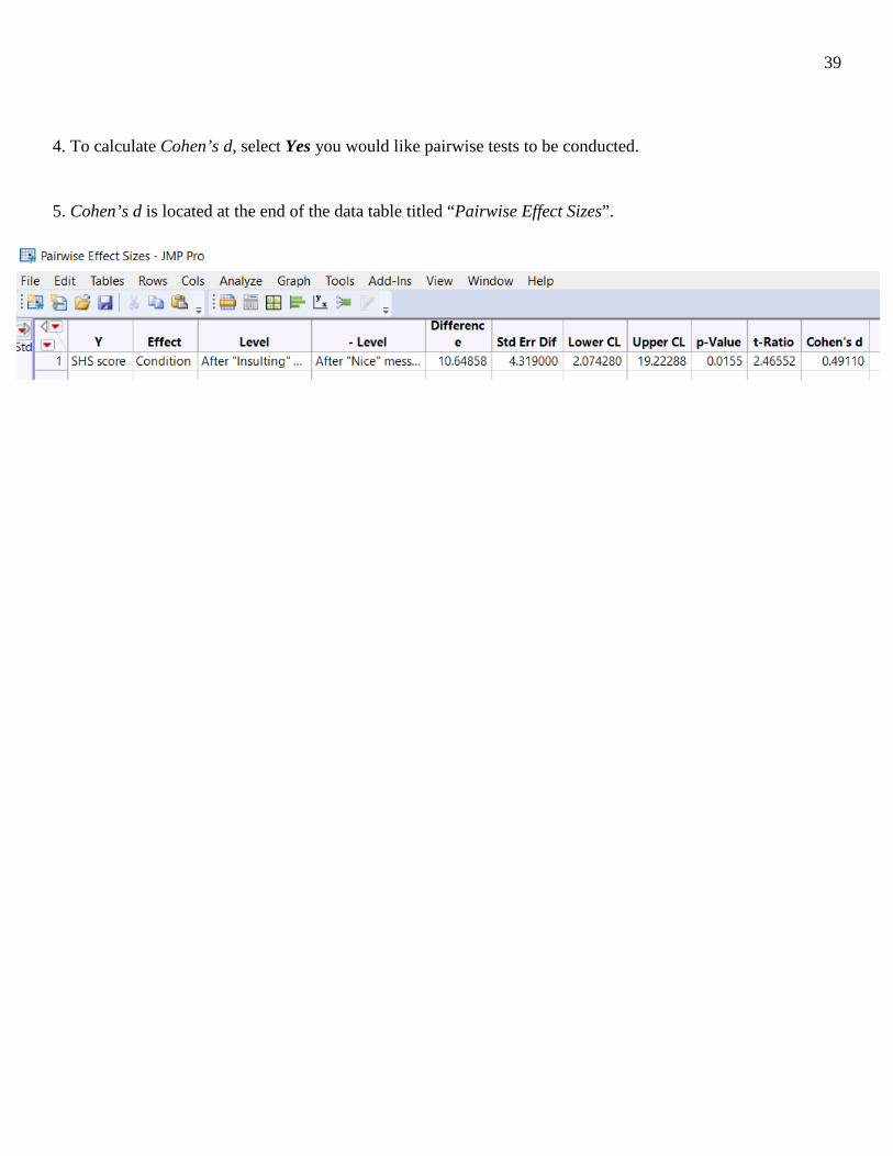
4. To calculate Cohen’s d, select Yes you would like pairwise tests to be conducted. 5. Cohen’s d is located at the end of the data table titled “Pairwise Effect Sizes”.

40

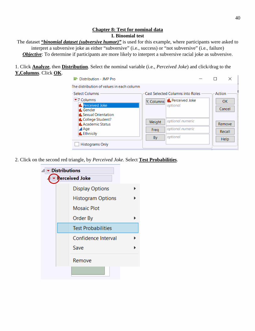
Chapter 8: Test for nominal data I. Binomial test

The dataset “binomial dataset (subversive humor)” is used for this example, where participants were asked to interpret a subversive joke as either “subversive” (i.e., success) or “not subversive” (i.e., failure)

Objective: To determine if participants are more likely to interpret a subversive racial joke as subversive.

1. Click Analyze, then Distribution. Select the nominal variable (i.e., Perceived Joke) and click/drag to the Y,Columns. Click OK. 2. Click on the second red triangle, by Perceived Joke. Select Test Probabilities.

41

3. Enter the hypothesized probabilities in the appropriate boxes and select an alternative hypothesis. For this example, we put in .5 for each. Note that the second and third choices are one-tail binomial tests based on the observed and hypothesized proportions in the second category. Click Done. 4. You can get exact confidence intervals for π by clicking red triangle, then Confidence Intervals, then the level of confidence you are interested in.

42

II. Chi square goodness-of-fit test

The dataset “chi square dataset (diversity)” is used for this example, where participants were asked to choose between either writing or verbally criticizing a proposed diversity initiative.

Objective: To determine if participants prefer one response option (i.e., verbal or written) over the other

1. Click Analyze, then Distribution. Select the nominal variable (i.e., Decision) and click/drag to the Y,Columns. Click OK. 2. Click on the second red triangle, by Decision. Select Test Probabilities.

43

3. Enter the hypothesized probabilities in the appropriate boxes and select an alternative hypothesis. For this example, we used .5 in both. Note that the second and third choices are one-tail binomial tests based on the observed and hypothesized proportions in the second category. Click Done.

44

Chapter 9: The Randomization/Permutation Model I. Approximate randomization test for difference between two groups

Objective: Conduct an approximate randomization test for the difference in SHS score between the two levels of message type (Nice Message, Insult Message)

1. Right-click on the Condition variable and select New Formula Column. Click on Random, then select Sample with Replacement. This adds a new column to the data table labeled as Resample[Condition]. 2. Click Analyze, then select Fit Y by X. 3. Select the predictor variable (i.e., Condition) and click/drag to the X,Factor box. Select the outcome variable (i.e., SHS score) and click/drag to the Y,Response box. Click OK.

45

4. Click on the Red Triangle, then select Means/ANOVA/Pooled t 5. Right-click on the F Ratio located in the Analysis of Variance section. Select Simulate. 6. Highlight Condition in the Column to Switch Out box; Resample[Condition] in the Column to Switch In. Set the number of samples you want (default is 2500). Click OK.

46

7. A new data table will appear. Click on Analyze and select Distribution. Click/drag Condition into the Y,Columns box and click OK. 8. The section labeled Simulation Results will contain the Empirical p-Values for two- and one-tailed tests and various confidence interval endpoints based on the original observed difference.

47

Chapter 10: Exploring Relationships Between Two Variables I. Approximate randomization test for correlation between two variables

Objective: Conduct an approximate randomization test for the correlation between SHS score and Arousal 1. Right-click on the Arousal variable and select New Formula Column. Click on Random, then select Sample with Replacement. This adds a new column to the data table labeled as Resample[Arousal]. 2. Click Analyze, then select Fit Y by X. 3. Select one of the variables (i.e., Resample[Arousal]) and click/drag to the X,Factor box. Select the other variable variable (i.e., SHS score) and click/drag to the Y,Response box. Click OK.

48

4. Click the red triangle and select Fit Line 5. Right-click on the R2 value located in the Summary of Fit section. Select Simulate. Click on SHS

49

6. Highlight Resample[Arousal] in the Column to Switch Out box; Resample[Arousal] in the Column to Switch In. Set the number of samples you want (default is 2500). Click OK. 7. A new data table will appear. Click on Analyze and select Distribution. Click/drag RSquare into the Y,Columns box and click OK 8. The section labeled Simulation Results will contain the Empirical p-Values for two- and one-tailed tests and various confidence interval endpoints based on the original observed difference.

50

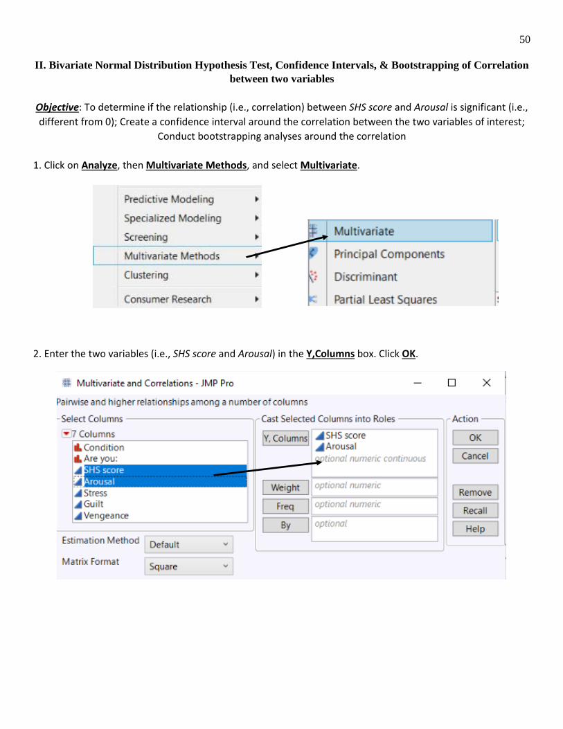
II. Bivariate Normal Distribution Hypothesis Test, Confidence Intervals, & Bootstrapping of Correlation between two variables

Objective: To determine if the relationship (i.e., correlation) between SHS score and Arousal is significant (i.e., different from 0); Create a confidence interval around the correlation between the two variables of interest;

Conduct bootstrapping analyses around the correlation 1. Click on Analyze, then Multivariate Methods, and select Multivariate. 2. Enter the two variables (i.e., SHS score and Arousal) in the Y,Columns box. Click OK.

51

3. Click on the red triangle by Multivariate. Select Correlation Probability and CI of Correlation.

4. The result is the following correlation, probability, and 95% confidence interval for the correlation.

52

5. To conduct a bootstrap, right-click on the correlation and select Bootstrap.

Input the number of samples wanted (default is 2500). Click OK.

6. A new data table will be generated with bootstrap samples in one column (BootID) and correlations in the second (Arousal SHS score). In this new data table, click on Analyze, select Distribution, and click/drag the second column (i.e., Arousal SHS score) into the Y,Columns box. Click OK. 7. The results provide various bootstrap confidence limits of the correlation between the two variables.

53

III. Spearman’s Rho & Kendall’s Tau

Objective: Conduct a Spearman’s Rho or Kendall’s Tau correlation on the variables SHS score and Arousal

1. Click on Analyze, then Multivariate Methods, and select Multivariate. 2. Enter the two variables (i.e., SHS score and Arousal) in the Y,Columns box. Click OK.

3. Click on the red triangle by Multivariate. Select Nonparametric Correlations, then select the correlation you want (we selected both Spearman’s and Kendall’s for this example).

54

4. Result is the following correlations and p-values.

55

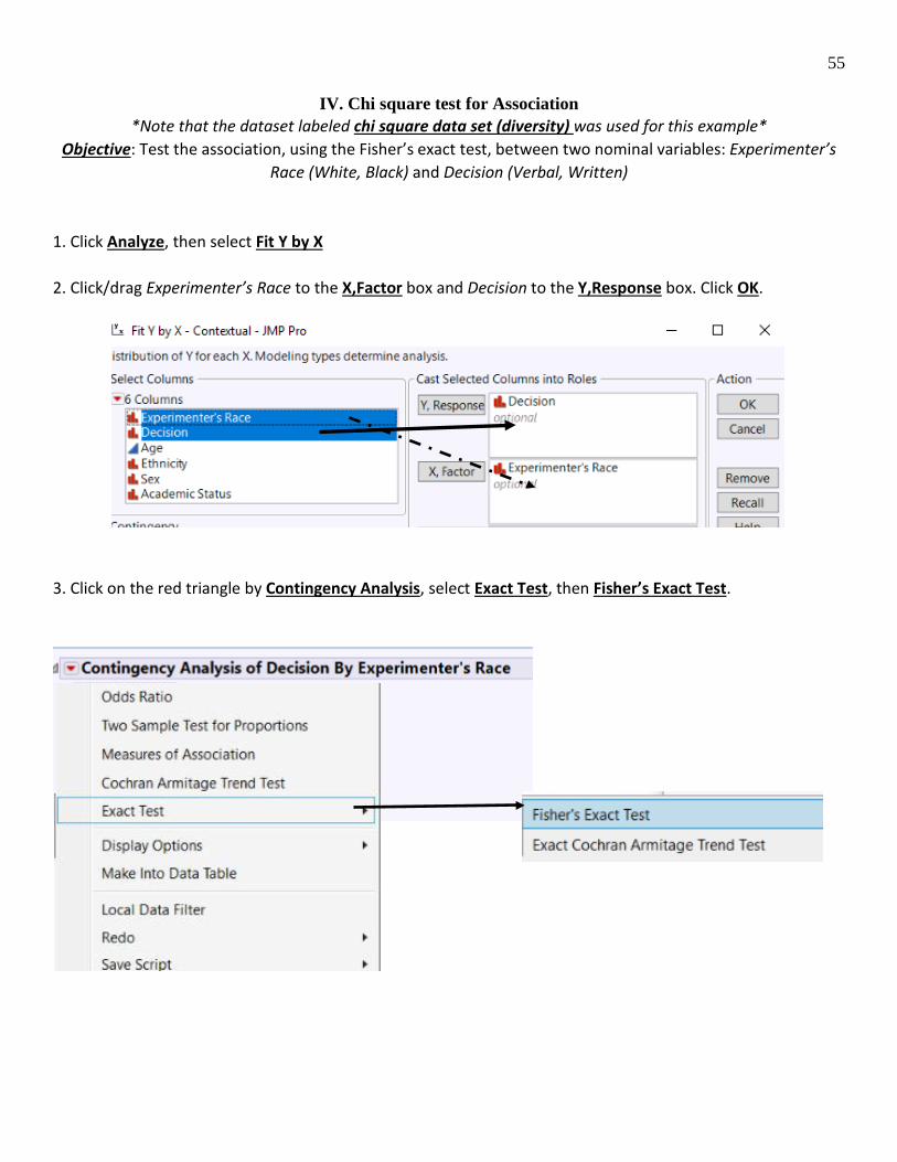
IV. Chi square test for Association *Note that the dataset labeled chi square data set (diversity) was used for this example*

Objective: Test the association, using the Fisher’s exact test, between two nominal variables: Experimenter’s Race (White, Black) and Decision (Verbal, Written)

1. Click Analyze, then select Fit Y by X 2. Click/drag Experimenter’s Race to the X,Factor box and Decision to the Y,Response box. Click OK. 3. Click on the red triangle by Contingency Analysis, select Exact Test, then Fisher’s Exact Test.

56

4. Results include a contingency table, test statistics, and results from Fisher’s Exact Test.

57

Chapter 11: Linear Regression Model I. Linear Regression: F and t statistics

Objective: To determine if the correlation coefficient between two variables in a regression analysis is significantly different than zero

1. Click Analyze, then select Fit Y by X. 2. Click/drag one variable (i.e., SHS score) to the Y,Response box and the other variable (i.e., Arousal) to the X,Factor Box. Click OK.

3. Click the red triangle and select Fit Line.

58

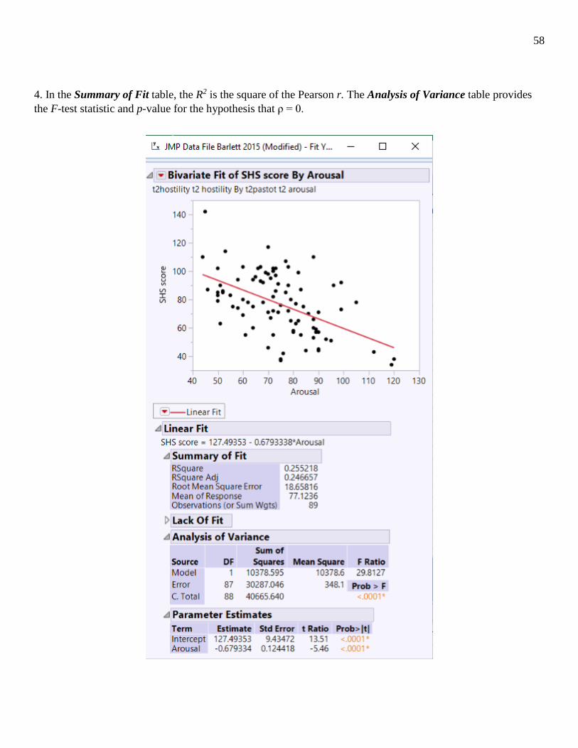
4. In the Summary of Fit table, the R2 is the square of the Pearson r. The Analysis of Variance table provides the F-test statistic and p-value for the hypothesis that ρ = 0.

59

Chapter 12: Closer Look at Linear Regression I. Checking assumptions in regression

Objective: Checking the assumptions for Regression – A. Independence of Observations

B. Linearity between predictor and criterion C. Variables are from a normal distribution

D. No multicollinearity issues among predictors E. Homoscedasticity

A. This is something that is determined and controlled for within the design of the study.

B. To check for linearity between the predictor and criterion, conduct a bivariate correlation using the

instructions from Chapter 10’s “Bivariate Normal Distribution Hypothesis Test, Confidence Intervals, & Bootstrapping of Correlation between two variables”. Using the magnitude of the correlation and associated p-value along with scatter plots to determine if a linear relationship exists.

C. To check that the variables each come from a normal distribution, graph their distribution using Chapter 2’s “Histograms” instructions.

D. To ensure no multicollinearity among multiple predictors, conduct a Linear Regression model and look at the Variance Inflation Factor (VIF) scores. **For this example, we will need at least 2 predictors in the regression model. Therefore, we will be using Arousal and Stress as predictors and SHS score as the criterion. ** 1. Click on Analyze, then Fit Model (you must use Fit Model even if you have only 1 predictor as in this example). 2. Click/drag the predictors (i.e., Arousal, Stress) into the Construct Model Effects box, and the criterion (i.e., SHS score) into the Y box. Click Run.

60

3. The VIF scores are located in the Parameter Estimates box (if they are not there, right-click in the Parameter Estimates box and select VIF). The “rule of thumb” is that VIF scores above 3 are indicators of multicollinearity among the predictors.

E. To test of homoscedasticity, look at the plot of the residuals of the model fit.

1. Click on Analyze, then Fit Model (you must use Fit Model even if you have only 1 predictor as in this example). 2. Click/drag the predictor (i.e., Arousal) into the Construct Model Effects box, and the criterion (i.e., SHS score) into the Y box. Click Run.

3. The Residual by Predicted Plot will be a part of the overall results.

61

II. Non-linear regression, Lack-of-fit

Objective: Conduct a non-linear regression and compare it to linear regression for the same variables to determine which model best fits the data

**Note that this example is using polynomial regression (quadratic). JMP also has non-linear modeling options for other types of non-linear regression models**

We will be using the Vengeance variable as a predictor and SHS score as the criterion. An initial graph (using Graph Builder), we see that there is a possible non-linear relationship between the two variables: 1. First conduct a linear regression model by selecting Analyze, then Fit Model. Input SHS score as Y and Vengeance as a Construct Model Effect. Click Run.

62

2. Results will include: A. Lack of Fit Results B. Plot of Residuals C. Summary of Fit D. ANOVA results for the model fit

63

3. Next conduct a second-degree (i.e., parabolic/quadratic) non-linear regression model by selecting Analyze, then Fit Model. Input SHS score as Y and Vengeance as a Construct Model Effect as before. Then, highlight both the Vengeance variable in the Columns box and the Vengeance variable in the Model Effects box AT THE SAME TIME by using the CTRL key on the keyboard. Click Cross, which will input the square of the Vengeance variable into the Model Effects box. Click Run.

64

4. The same output will result as before: A. Lack of Fit Results B. Plot of Residuals C. Summary of Fit D. ANOVA results for the model fit

5. Note how the non-linear regression model is a better fit, in both the R2 values as well as the Lack of Fit tests.

65

Chapter 13: Another Way to Scale the size of Treatment Effects I. Point biserial r

Objective: Test relationship between a dichotomous variable (i.e., Message Type: Nice, Insult) and a continuous variable (i.e., SHS score).

1. Click Analyze, then select Fit Y by X. 2. Select the predictor variable (i.e., Condition) and click/drag to the X,Factor box. Select the outcome variable (i.e., SHS score) and click/drag to the Y,Response box. Click OK. 3. Click on the Red Triangle, then select Means/ANOVA/Pooled t

66

4. Locate R2 in the Summary of Fit section. The Pearson r is the square root of R2 : square root of 0.060139 = 0.2452

67

Chapter 14: Analysis of Variance (ANOVA) I. One-way ANOVA

Objective: Compare the mean of SHS score between two levels of Message type (Nice, Insult) 1. Click Analyze, then select Fit Model. 2. Click/drag the categorical variable (i.e., Condition) to the Construct Model Effects box and the continuous variable (i.e., SHS score) to the Y box. Click Run. 3. The Analysis of Variance section contains the Source of Variance, degrees of freedom, Sum of Squares, Mean Square, F-ratio, and associated p-value.

68

II. Relational Effect Size Measures Eta squared, Partial eta squared, Omega squared

Objective: To produce standardized effect size after comparing the State Hostility score (SHS score) between the two levels of Message (Insult, Nice)

**This requires the Calculate Effect Sizes Add-In, which can be downloaded from https://community.jmp.com/t5/JMP-Add-Ins/Calculate-Effect-Sizes-Add-in/ta-p/22642 **

1. Click on Analyze, then select Fit Model (you must select Fit Model and not Fit Y by X) 2. Select the predictor variable (i.e., Condition) and click/drag to the Model Effects box. Select the outcome variable (i.e., SHS score) and click/drag to the Y box. Click OK. 3. Go back to the data table, click Add-Ins, and select the appropriate add-in (i.e., Calculate Effect Sizes). Select the Least Squares Report. 4. Select Yes if you would like pairwise tests to be conducted, Select No if you want only the effect sizes for the model produced.

https://community.jmp.com/t5/JMP-Add-Ins/Calculate-Effect-Sizes-Add-in/ta-p/22642

69

5. A new data table will generate with the effect sizes in the columns.

70

III. Approximate Randomization Test for ANOVA Objective: To determine if Message Type (Nice, Insult) has an effect on Stress.

1. Right-click on Condition column in the data set, and select New Formula Column. Click on Random, then select Sample with Replacement. A new column will be added to the data set titled Resample[Condition]. 2. Click on Analyze, then select Fit Y by X. 3. Select the predictor variable (i.e., Condition) and click/drag to the X,Factor box. Select the outcome variable (i.e., Stress) and click/drag to the Y,Response box. Click OK.

71

4. Click on the Red Triangle, then select Means/ANOVA/Pooled t. 5. Right-click on the F Ratio located in the Analysis of Variance section. Select Simulate. 6. Highlight Condition in the Column to Switch Out box; Resample[Condition] in the Column to Switch In. Set the number of samples you want (default is 2500). Click OK.

72

7. A new data table will appear. Click on Analyze and select Distribution. Click/drag Condition into the Y,Columns box and click OK. 8. The section labeled Simulation Results will contain the Empirical p-Values for two- and one-tailed tests and various confidence interval endpoints based on the original observed difference.

73

IV. Two-way ANOVA Objective: Compare the mean of SHS score between Message type (Nice, Insult) and Gender (Male, Female)

1. Click Analyze, then select Fit Model. 2. Click/drag the continuous variable (i.e., SHS score) to the Y box. Next click/drag the 2 categorical variables (i.e., Condition, Gender) to the Construct Model Effects box. Then, highlight both the Condition variable in the Columns box and the Gender variable in the Model Effects box AT THE SAME TIME by using the CTRL key on the keyboard. Click Cross, which will insert the two-way interaction of the two variables into the Model Effects box. Click Run.

74

3. The Analysis of Variance section contains variance information regarding the model as well as the F-ratio and associated p-value. The Effect Tests box contains the variance information regarding main effects and interactions in the model. The Parameter Estimates box contains estimate information regarding differing levels of each main effect and interaction within the model. **Note that JMP uses effect coding for categorical predictors. In this example, Insult is coded as 1 and Nice is coded as –1; Male is coded as 1 and Female is coded as –1.

75

Chapter 15 – Multiple Regression & Beyond

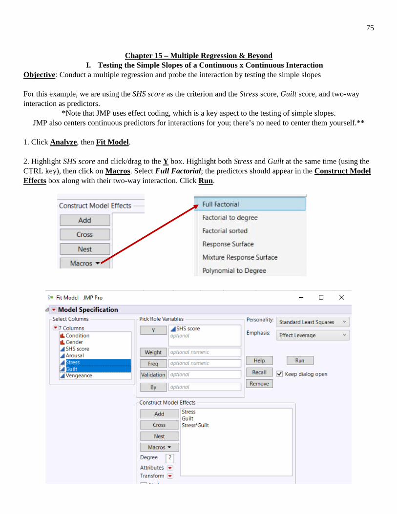
I. Testing the Simple Slopes of a Continuous x Continuous Interaction Objective: Conduct a multiple regression and probe the interaction by testing the simple slopes For this example, we are using the SHS score as the criterion and the Stress score, Guilt score, and two-way interaction as predictors.

*Note that JMP uses effect coding, which is a key aspect to the testing of simple slopes. JMP also centers continuous predictors for interactions for you; there’s no need to center them yourself.**

1. Click Analyze, then Fit Model. 2. Highlight SHS score and click/drag to the Y box. Highlight both Stress and Guilt at the same time (using the CTRL key), then click on Macros. Select Full Factorial; the predictors should appear in the Construct Model Effects box along with their two-way interaction. Click Run.

76

3. The results will include the following: Summary of Fit Analysis of Variance (for the Model) Parameter Estimates Effect Tests Even though there is not a significant two-way interaction, we are going to probe the interaction for the purposes of this example. We will test the Simple Slopes of Guilt at different levels of Stress: 1 standard deviation below the mean, at the mean, and 1 standard deviation above the mean. You can find the standard deviation by using the Distribution function in JMP: the SD of Stress is 6.3698

77

4. Click the Red Triangle by Response SHS score. Select Estimates, then Custom Test. 5. To test the simple slopes of Guilt, we will need to put in our own parameters at the different levels of Stress. Since we are testing at 3 different levels (1 SD below, 1 SD above, and mean), click Add Column to add 2 additional Parameter columns.

6. a. The first column we input the parameters for testing the slope of Guilt at 1 SD below the mean of Stress (i.e., –6.3698) b. The second column we input the parameters for testing the slope of Guilt at the mean of Stress (i.e., 0) c. The third column we input the parameters for testing the slope of Guilt at 1 SD above the mean of Stress (i.e., 6.3698).

78

7. Click Done. The results will generate below using the parameters we inputted.

a. The value of 1.9297 is the slope of Guilt at 1 SD below the mean of Stress; this is significantly different than a slope of 0 (t = 2.54, p = .01) b. The value of 1.6285 is the slope of Guilt at the mean of Stress; this is significantly different than a slope of 0 (t = 2.84, p = .01) c. The value of 1.3272 is the slope of Guilt at 1 SD above the mean of Stress; this is significantly different than a slope of 0 (t = 2.36, p = .02)

79

II. Testing the Simple Slopes of a Categorical x Continuous Interaction Objective: Conduct a multiple regression and probe the interaction by testing the simple slopes For this example, we are using the SHS score as the criterion and the Arousal score, Condition (Message Type: Insult, Nice), and two-way interaction as predictors.

*Note that JMP uses effect coding, which is a key aspect to the testing of simple slopes.** 1. Click Analyze, then Fit Model. 2. Highlight SHS score and click/drag to the Y box. Highlight both Condition and Arousal at the same time (using the CTRL key), then click on Macros. Select Full Factorial; the predictors should appear in the Construct Model Effects box along with their two-way interaction. Click Run.

80

3. The results will include the following: Summary of Fit Analysis of Variance (for the Model) Parameter Estimates Effect Tests Even though there is not a significant two-way interaction, we are going to probe the interaction for the purposes of this example. We will test the Simple Slopes of Arousal at the 2 levels of Condition. Note here that JMP, using effect coding, has coded Insult as 1 and Nice as –1. 4. Click the Red Triangle by Response SHS score. Select Estimates, then Custom Test.

81

5. To test the simple slopes of Arousal, we will need to put in our own parameters at the 2 levels of Condition (Insult, Nice). Click Add Column to add 1 additional Parameter column.

6. a. The first column we input the parameters for testing the slope of Arousal at the level of Insult. b. The second column we input the parameters for testing the slope of Arousal at the level of Nice. 7. Click Done. The results will generate below using the parameters we inputted. a. The value of –0.4679 is the slope of Arousal in the Insult Message Condition; this is significantly different than a slope of 0 (t = –2.74, p = .01) b. The value of –0.8753 is the slope of Arousal in the Nice Message Condition; this is significantly different than a slope of 0 (t = –5.34, p < .0001)

manual for using jmp with principles & methods of

Documents