i

Manufacturing Tolerance Cost Minimization

Using Discrete Optimization For Alternate Process Selection

ADCATS Report No. 87-4

Bruce G. Loosli, graduate student

Department of Mechanical Engineering

Brigham Young University

MS Thesis sponsored by ADCATS

August 1987

ABSTRACT

The allocation of tolerances among the components of a mechanical assembly can significantly affect the resulting manufacturing costs. Using a cost-vs.-tolerance function for each dimension, the least cost tolerance allocation may be determined analytically by the method of Lagrange multipliers. When alternative manufacturing processes are available for some of the components, the analysis may be repeated for each of the possible combinations of processes to determine the least cost production method as well as tolerances. However, the number of combinations increase geometrically, becoming very large for assemblies of moderate complexity.

Several methods are described for systematically searching for the minimum cost process set without having to exhaustively try every possible combination. Two promising methods have been quantitatively tested and compared to an exhaustive search. The number of combinations and CPU time are greatly reduced.

When a preferred tolerance range is specified for each process, the process search methods have difficulty due to the presence of local minima. A procedure for applying process tolerance constraints was developed which greatly increases the likelihood of finding the absolute minimum cost.

ii

Table of Contents

LIST OF FIGURES .........................................................................................................v

LIST OF TABLES...........................................................................................................vi

ACKNOWLEDGEMENTS.............................................................................................7

1.0 INTRODUCTION ...............................................................................................8

1.1 Single Process Optimization....................................................................10

1.2 Alternate Process Selection Methods.......................................................11

1.2.1 Balas Algorithm...........................................................................11

1.2.2 Branch and Bound .......................................................................14

1.3 Thesis Objectives .....................................................................................15

1.4 Overview of Results.................................................................................15

2.0 MODEL DEVELOPMENT.................................................................................16

2.1 Assembly Cost Function..........................................................................16

2.2 Assembly Tolerance Constraint...............................................................17

2.3 Lagrange Multiplier Optimum Solution ..................................................18

2.0 MODEL DEVELOPMENT.................................................................................20

2.1 Assembly Cost Function..........................................................................20

2.2 Assembly Tolerance Constraint...............................................................21

2.3 Lagrange Multiplier Optimum Solution ..................................................21

3.0 SOLUTION METHODS .....................................................................................24

3.1 Multiple Cost Curve Problem..................................................................24

iii

3.2 Experience with Branch and Bound ........................................................25

3.3 Exhaustive Search....................................................................................26

3.4 Process Selection by Following the Lowest Curve Profile......................28

3.5 Univariate Search with Tolerance Allocation..........................................29

3.6 Continued Univariate Search ...................................................................32

3.7 Applying Tolerance Constraints by End-fixing.......................................33

3.8 Incremental End-fixing ............................................................................33

3.9 Process Search Performance with End-fixing..........................................35

3.9.1 Exhaustive Search Method ..........................................................36

3.9.2 Bottom Curve Following Method................................................36

3.9.3 Univariate Search Method ...........................................................36

4.0 RESULTS ............................................................................................................38

4.1 Unconstrained Problems ..........................................................................38

4.2 Problems with Process Constraints..........................................................40

4.3 Effects of Problem Size ...........................................................................43

4.4 Limitations ...............................................................................................44

5.0 CONCLUSIONS AND RECOMMENDATIONS ..............................................46

5.1 Conclusions..............................................................................................46

5.2 Recommendations for Other Possible Methods.......................................47

5.2.1 Simulated Annealing Possibility..................................................47

5.2.2 Gradient Possibility......................................................................48

5.3 Need for Good Data .................................................................................48

iv

5.4 CATS.BYU Recommendations ...............................................................49

5.4.1 Reference Handbook Data ...........................................................50

5.4.2 Flexible Control Features.............................................................50

REFERENCES ................................................................................................................51

APPENDIX I ..................................................................................................................52

APPENDIX II .................................................................................................................62

v

LIST OF FIGURES

Figure page

Figure 1.1. Sample Assembly for Tolerance Analysis ....................................................8

Figure 1.2. Sample Process Cost Curve...........................................................................10

Figure 1.3. Bounded Process Cost Curves.......................................................................14

Figure 3.1. Form of Alternate Process Cost Curves ........................................................24

Figure 3.2. Assembly Tolerance Cost Contours ..............................................................26

Figure 3.3. Example Problem Process Cost Curves ........................................................27

Figure 3.4. Exhaustive Search Tree .................................................................................28

Figure 3.5. Sample Process Cost Curve Switch...............................................................29

Figure 3.6. Sample Tree for Univariate Search ...............................................................31

Figure 3.7. Incremental End-fixing..................................................................................35

Figure 4.1. CPU Usage Comparison Chart......................................................................39

Figure 4.2. CPU Usage for Problems T,U, and UU.........................................................41

Figure 4.3. Assembly Tolerance Costs for T and U ........................................................43

vi

LIST OF TABLES

Table page

Table 4.1. Performance Values for Problems A-I............................................................39

Table 4.2. Performance Data for Problems T,U, and UU................................................42

7

ACKNOWLEDGEMENTS

Special thanks to Dr. Chase for his understanding assurances and insightful

dreams. Through his efforts I was given a means to support my family throughout the

duration of my master’s degree. And to my fellow workers on the CATS program, I give

thanks for their help and wishes of good luck in implementing my work into CATS.

I thank Dave Larsen and Tim McClain for their considerate suggestions and

support when the times got tough. Their smiles and very poor humor gave me the

necessary entertainment to keep my sanity.

Finally, I thank my wife, Connie, for her support both physical and emotional.

She helped keep our personal affairs in order during the final weeks of thesis preparation

and very rarely complained. Thanks to my son, James, who still does not know why I

always had to leave him. I hope that now we can spend time together every day.

8

1.0 INTRODUCTION

The specification of tolerances on part dimensions can have a large impact on

production cost. By properly allocating tolerances among the components of mechanical

assemblies, costs may be lowered without a great deal of overhead. For that reason,

tolerance analysis and tolerance allocation for cost minimization is becoming a prominent

topic of discussion.

Tolerance analysis is the analytical method of estimating tolerance accumulation

in mechanical assemblies. Through tolerance analysis, critical clearances may be

maintained and part interchangeability can be assured. For example, given the

configuration shown in Figure 1.1 consisting of parts 1, 2, and 3 fitting together and

required to fit inside part 4.

Part 1Part 2

Part 3

Part 4

Clearance

a) Sample Assembly

Clearance

1.000 ± Tol 1 1.875

± Tol 2 0.750 ± Tol 3

3.650 ± Tol 4

0.025 ± 0.006

b) Sample Assembly Tolerance Stack

Figure 1.1. Sample Assembly for Tolerance Analysis

Parts 1, 2, 3, and 4 all have dimensions and tolerances associated with them. The

tolerance values imply that there is some variability in the actual dimensions of the parts,

or from the other side, a tolerance value means that the part dimension can only be

assumed to be within a specified range. The sample assembly in Figure 1.1 demonstrates

9

why one must consider the effects of tolerance accumulation to see if the parts will fit

together properly.

For tolerance analysis, the assembly tolerance is specified as the overall

constraint. In Figure 1.1, the specified assembly tolerance is the tolerance on the

clearance. The magnitude of the four componenet tolerances must be assigned by the

designer, subject to the assembly tolerance constraint. That is, the sum of the component

tolerances, parts 1 to 4, must be less than or equal to the assembly tolerance, clearance, in

order to fit.

tolqasm • ∑

i=1

n

tolqi (Eq. 1.1)

or

tol asm •

∑i=1

n

tolqi

1q

(Eq. 1.2)

N is the number of parts in the assembly. For the case in Figure 1.1, n = 4. The q

exponent specifies the addition model. When q = 1, worst limit tolerancing is used, if

q = 2, statistical tolerancing results. Statistical analysis assumes a normal distribution of

part tolerances, allowing for larger tolerances than with worst limit because of the low

probability that all worst case parts will be selected for assembly at once. (Fortini1)

Given the constraint of Eq. 1.2, all component tolerances could be evenly

allocated to spread the available assembly tolerance across all parts. However, each

component tolerance may have a different manufacturing cost associated with it due to

part complexity or process differences. If tolerance costs are considered in the tolerance

allocation, the component tolerances may be allocated to minimize the manufacturing

cost of an assembly .

10

Tol

eran

ce C

ost

Tolerance

Figure 1.2. Sample Process Cost Curve

The cost of producing a given tolerance is of the form displayed in Figure 1.2. As

the tolerance increases, the cost goes down. If more than one process is capable of

producing the same part dimension, then the cost curves for each available process for

producing the part could be included for comparison. In this way, the least cost

manufacturing processes for an assembly may be selected in addition to the minimum

cost tolerance allocation.

1.1 Single Process Optimization

Spotts10 and Speckhart12 developed models for solutions to minimum cost

tolerance allocation. They both assumed that the processes to be used were already

selected. Spotts modeled the tolerance cost as varying as the inverse of the tolerance

squared, while Speckhart used an exponential form. However, both presented the idea

that a closed form solution using Lagrange multipliers was efficient and well suited to the

tolerance allocation problem.

The method of Lagrange multiplier optimization of tolerance allocation is also

used in the CATS.BYU2 software. The CATS.BYU program has been under

development since 1984 and was first released in 1986. It is a basic tolerance analysis

program for linear tolerance stack problems. In the current edition (Version 1.1), cost

allocation can be performed given a single process cost curve for each component and

requiring the same form for each process cost curve within an assembly.

11

Because of the great desire to minimize costs in the manufacturing arena, CATS

has received a welcome response. However, sponsors of the CATS.BYU program have

requested many enhancements; including the ability to handle multiple cost curves to

assist in process selection has often been requested and was the impetus behind this

master’s thesis.

Although the Lagrange multiplier technique is efficient for tolerance allocation, it

is important to extend the capability to allow consideration of alternate processes. The

Lagrange multiplier technique does not permit alternate process selection by itself.

However, it can be combined with other methods to successfully solve the problem.

1.2 Alternate Process Selection Methods

Because the tolerance allocation problem could be solved in closed form, the

optimum process selection could be treated as a discrete combinatorial problem. For

every combination of process cost curves selected, an assembly tolerance cost could be

used as the objective function and compared with other costs from different combinations

until the global optimum was discovered. However, for each combination a complete

tolerance allocation must be done before the assembly tolerance cost can be compared.

Although exhaustively searching (trying every process curve combinations) would

provide the global optimum to a problem, it may become too costly or too time-

consuming to perform all of the evaluations necessary to check each possibility.

Therefore, discrete optimization techniques can be used to lower the number of cases to

be checked and thus reduce the computation time and expense.

1.2.1 Balas Algorithm

One method for including process selection in a tolerance allocation problem is

the Balas algorithm to solve a completely discrete problem. Huang and Ostwald11

approached the problem using the Balas algorithm. The Balas algorithm was designed to

do a selective search over the entire combination space to find the global optimum. The

method involves the following steps.

1) The designer selects combinations of tolerance values and associated process

costs to represent the continuous process cost curves at discrete points.

12

2) An objective function is formed by summing the possible discrete cost terms

for all parts in the assembly.

3) Binary coefficients are placed in front of each tolerance-cost value and the

coefficients are turned on and off ( 1 and 0 ) to select tolerance combinations

across the entire problem.

4) Tolerances corresponding to the selected costs are summed and compared to

the specified assembly tolerance. Invalid combinations are eliminated.

5) By requiring that all coefficients for one part add up to one, the method is

constrained to have only one point for each part activated at a time.

6) Then a systematic search for the minimum cost combination of process-costs

satisfying the constraints is done.

The Balas problem may be expressed algebraically as follows:

Minimize the objective function,

Cost = ∑ i = 1

n bi Ci (Eq. 1.3)

subject to the constraints,

tolasm • ∑ i = 1

n

∑j = 1

mi

bij tij (Eq. 1.4)

∑j = 1

mi bij = 1 (i = 1,...,n) (Eq. 1.5)

bij =

1 on

0 off (j = 1,...,mi), (i = 1,...,n) (Eq. 1.6)

(n = number of parts, mi = number of discrete points for parti)

13

Hauglund9 compared the Balas algorithm against a continuous approximation

method to determine the best method for process selection and tolerance allocation. He

also demonstrated a continuous model of the alternate process cost curves. Both methods

were compared with the exhaustive search in CPU time necessary for solution as well as

accuracy and analysis efficiency. The continuous and Balas methods both proved to be

more CPU intensive than the exhaustive search. However, the continuous model did

become more efficient than the exhaustive search as the number of process cost curves

exceeded thirty-five. A drawback of the Balas algorithm was that discrete points had to

be selected from the process cost curves to generate a totally discrete problem. In

industry, cost curves tend to be at least piecewise continuous and hence would lose some

continuity depending on the number of points used to represent the curves.

Hauglund’s work showed that the exhaustive combinatorial search actually proved

more efficient than either the Balas algorithm or the continuous problem representation

until the number of curves began exceeding the thirty-five to forty limit. In this case, the

number of combinations exceeded one million and the continuous solution became more

efficient. In all three methods, the CPU usage was extensive and very costly and viewed

as unacceptable for design iterations. Hauglund also had difficulty evaluating problems

when constraints were placed on the process tolerance ranges. Process tolerance

constraints increased the complexity of the problem and led sometimes to no solution

being found. The most difficult case occurs when the tolerance ranges of the alternate

process do not overlap, as shown in Figure 1.3. In Figure 1.3, process cost curves for one

part are represented as continuous curves; the specified valid range of process tolerances

is shaded.

14

Tolerance Range Tolerance Range Tolerance Range

Process 3

Process 2

Process 1

Tol

eran

ce C

ost

Tolerance

Figure 1.3. Bounded Process Cost Curves

1.2.2 Branch and Bound

Another discrete optimization procedure is the Branch and Bound algorithm. It

looked promising as a method for process selection. Branch and Bound algorithms may

be used on discrete problems with multiple available discrete combinations if the

alternatives can be represented in a tree-like structure. Searches are done across single

tree levels. Only those branches that have the best objective function values are continued

to be evaluated while the expensive branches are pruned from the search.

Preliminary studies caused us to abandon the Branch and Bound method.

Although the multiple processes under consideration for this thesis could be represented

by a combination tree, the re-allocation of tolerances for each combination prevented the

Branch and Bound method from behaving well. As tolerances were allocated, processes

could be switched or out-of-range tolerances would need to be fixed at process limits.

This meant that the constraints on the problem could be changing as a function of the

tolerance allocation. A better method of considering the effects of tolerance allocation on

process selection and overall assembly cost was needed.

15

1.3 Thesis Objectives

The objectives of this thesis include:

1) Find a more efficient solution method for the combined discrete process

selection and tolerance allocation optimization problem arising from

alternative process availability.

2) Investigate behavior of methods when non-continuous process tolerance

ranges are applied.

3) Recommend a method for use in CATS.BYU.

1.4 Overview of Results

1) Branch and Bound solution method was determined to be unusable for this

application.

2) Various new combinatorial search methods were tried. A common set of test

problems was used to test each method. Comparisons were made of CPU time

and total number of combinations tried to find the minimum cost solution.

Three methods tested in detail are called:

a) Exhaustive search method

b) Bottom Curve Follower method

c) Univariate search method

The exhaustive search was used for comparison.

3) A method for handling process tolerance limits was developed for use with the

combinatorial search methods. It is based on first solving the unconstrained

problem for a particular process combination, then bringing any out-of-bound

tolerances in-bounds by gradually applying the constraints.

4) It was determined that an extended univariate search should be used for

problems when the number of exhaustive search combinations exceeds 50.

The exhaustive search is still the only method that can guarantee the absolute

minimum cost for a given assembly, but the continued univariate search

16

provided the same accuracy as the exhaustive search on large problems at a

fraction of the CPU time.

5) Suggestions for implementation in the CATS.BYU program are included to

allow the procedures mentioned in this thesis to be included in the near future.

2.0 MODEL DEVELOPMENT

Development of the ground work for this thesis consisted of deciding on the form

of the tolerance cost relationship in order to develop an objective function and then

including the tolerance constraints in the problem.

2.1 Assembly Cost Function

The cost verses tolerance equation for a single process was represented in the

following form:

Costi = A

i + B

i Tol

i

p (Eq. 2.1)

This cost curve model was patterned after the work done by Spotts10. The model consists

of a fixed cost offset (A) plus a cost coefficient (B) times the tolerance (Tol) raised to a

power (p) as shown in equation 2.1. Spotts recommended an exponent of p = -2. Chase

and Greenwood2 recommended p = -1. Chase and Greenwood also noted that they

recommended their model on the basis of limited data. However, it is believed that using

the same form of the cost equation and allowing non-integer values of p, most process

cost curves could be approximated by equations of this form, if only piecewise. Hence,

the modified form of the cost function is used exclusively in the development of the

theory and problems for this thesis. The generalized cost equation for a given tolerance is

then represented in the following form:

Costi = A

i + B

i Tol

i

pi (Eq. 2.2)

The tolerance cost of an assembly is the sum of the individual part costs.

Costasm

= ∑i=1

n Cost

i = ∑

i=1

n

A

i + B

i Tol

i

pi (Eq. 2.3)

(n = number of parts)

17

Minimizing the assembly tolerance cost entails minimizing equation 2.3 by selection of

an appropriate set of component tolerances. Of course, the absolute minimum would

occur as the component tolerances approached infinity given no restriction on tolerance

magnitudes. However, the component tolerances are constrained to meet some

performance criteria.

2.2 Assembly Tolerance Constraint

The performance criteria of a tolerance analysis problem is that the sum of the

individual component tolerances raised to the corresponding power must be less than or

equal to the specified assembly tolerance raised to that same power.

tol qasm • ∑

i=1

n

fx

i

q

tolqi (Eq. 2.4)

or

tol asm •

∑

i=1

n

fx

i

q

tolqi

1 q

(Eq. 2.5)

q =

1 : worst case

2 : root sum squared

Equation 2.5 describes how tolerance accumulates in a mechanical assembly. Common design assumptions are q = 1: worst case analysis, assuming tol

i selected such

that they will meet assembly tolerance limits even when all components are produced at their size limits; or q = 2: root-sum-squared analysis, assuming tol

i selected as having

random variations in component dimensions, leading to dimensional variations adding

statistically as independent variations. The symbol (f) represents assembly function

dimension, and the partial derivative with respect to the part dimension (x) in equation

2.5 is the sensitivity of the tolerance stack to each individual tolerance, fxi

q

. The

sensitivity only arises in 2-D and 3-D problems as the sensitivity of a 1-D problem is

equal to 1.0.

18

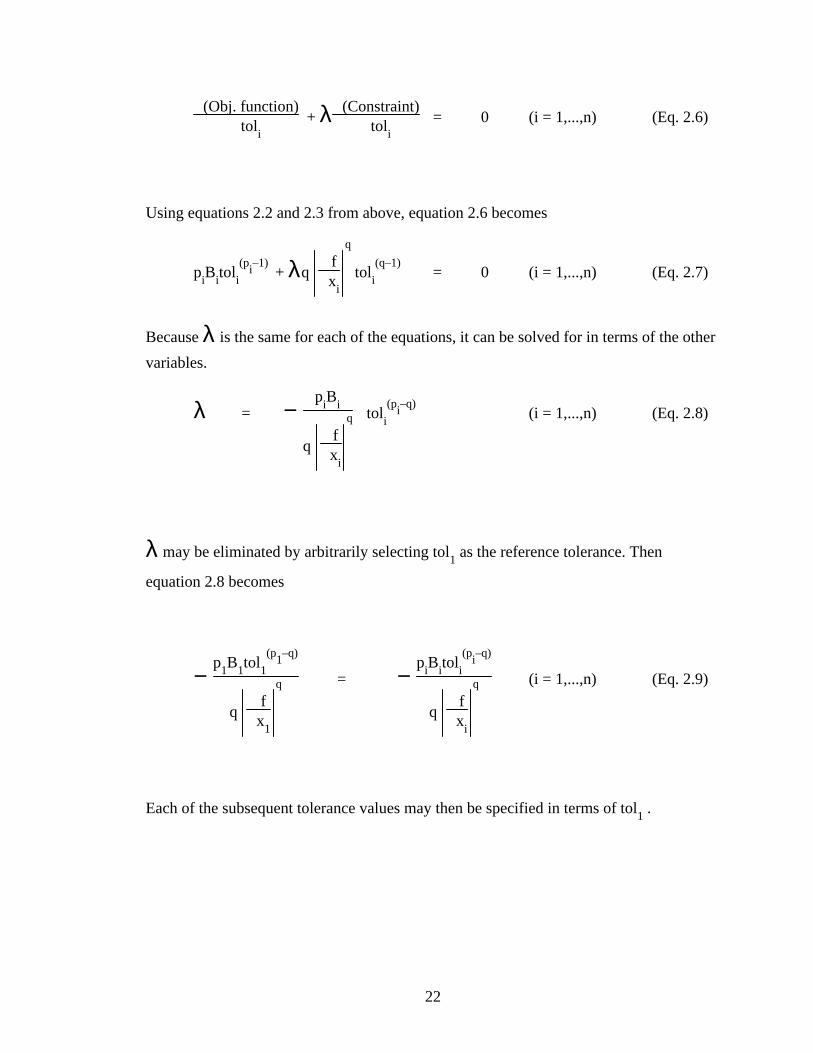
2.3 Lagrange Multiplier Optimum Solution

In order to minimize the tolerance cost, the Lagrange multiplier technique can be

used on each of the individual part equations.

(Obj. function)

toli

+ λ (Constraint)tol

i = 0 (i = 1,...,n) (Eq. 2.6)

Using equations 2.2 and 2.3 from above, equation 2.6 becomes

piB

itol

i

(pi–1)

+ λq

fx

i

q

toli

(q–1)

= 0 (i = 1,...,n) (Eq. 2.7)

Because λ is the same for each of the equations, it can be solved for in terms of the other

variables.

λ = − p

iB

i

q fx

i

q toli

(pi–q)

(i = 1,...,n) (Eq. 2.8)

λ may be eliminated by arbitrarily selecting tol1 as the reference tolerance. Then

equation 2.8 becomes

− p

1B

1tol

1

(p1–q)

q f

x1

q = − p

iB

itol

i

(pi–q)

q fx

i

q (i = 1,...,n) (Eq. 2.9)

Each of the subsequent tolerance values may then be specified in terms of tol1 .

19

toli =

p1

pi B

1

Bi

fx

i

q

fx

1

q tol1

(p1–q)

1

pi–q

(i = 2,3,...n) (Eq. 2.10)

Substitution of the tolerance values into the constraint equation leads to the following

equation.

tolqasm =

f

x1

q

tolq1 + ∑

i=2

n

fx

i

q

p1

pi B

1

Bi

fx

i

q

fx

1

q tol1

(p1–q)

qp

i–q

(Eq. 2.11)

An iterative solution for the value of tol1 can then be used to satisfy the constraint

equation and determine the set of component tolerances which yield the minimum cost.

This method gives a closed form solution to allocating the tolerances and reduces the search to a value of tol

1 that satisfies the tolerance constraint equation. This represents an

extension of Spott’s work, as he assumed all the pi = -2.0, which did not require an

iterative solution for tol1.

However, the Lagrange multiplier algorithm does not include provisions for

process tolerance limits. It also does not work directly with inter-dependent loops, where

two or more tolerance analysis loops have some shared parts. Only one assembly can be

analyzed at a time. Analyzing each loop separately and then fixing the shared part

tolerances at the minimum overall values can be used to overcome this weakness, but

Hauglund9 mentions that it may not be as efficient as a generalized optimization

algorithm.

20

2.0 MODEL DEVELOPMENT

Development of the ground work for this thesis consisted of deciding on the form

of the tolerance cost relationship in order to develop an objective function and then

including the tolerance constraints in the problem.

2.1 Assembly Cost Function

The cost verses tolerance equation for a single process was represented in the

following form:

Costi = A

i + B

i Tol

i

p (Eq. 2.1)

This cost curve model was patterned after the work done by Spotts10. The model consists

of a fixed cost offset (A) plus a cost coefficient (B) times the tolerance (Tol) raised to a

power (p) as shown in equation 2.1. Spotts recommended an exponent of p = -2. Chase

and Greenwood2 recommended p = -1. Chase and Greenwood also noted that they

recommended their model on the basis of limited data. However, it is believed that using

the same form of the cost equation and allowing non-integer values of p, most process

cost curves could be approximated by equations of this form, if only piecewise. Hence,

the modified form of the cost function is used exclusively in the development of the

theory and problems for this thesis. The generalized cost equation for a given tolerance is

then represented in the following form:

Costi = A

i + B

i Tol

i

pi (Eq. 2.2)

The tolerance cost of an assembly is the sum of the individual part costs.

Costasm

= ∑i=1

n Cost

i = ∑

i=1

n

A

i + B

i Tol

i

pi (Eq. 2.3)

(n = number of parts)

Minimizing the assembly tolerance cost entails minimizing equation 2.3 by selection of

an appropriate set of component tolerances. Of course, the absolute minimum would

occur as the component tolerances approached infinity given no restriction on tolerance

21

magnitudes. However, the component tolerances are constrained to meet some

performance criteria.

2.2 Assembly Tolerance Constraint

The performance criteria of a tolerance analysis problem is that the sum of the

individual component tolerances raised to the corresponding power must be less than or

equal to the specified assembly tolerance raised to that same power.

tol qasm • ∑

i=1

n

fx

i

q

tolqi (Eq. 2.4)

or

tol asm •

∑

i=1

n

fx

i

q

tolqi

1 q

(Eq. 2.5)

q =

1 : worst case

2 : root sum squared

Equation 2.5 describes how tolerance accumulates in a mechanical assembly. Common design assumptions are q = 1: worst case analysis, assuming tol

i selected such

that they will meet assembly tolerance limits even when all components are produced at their size limits; or q = 2: root-sum-squared analysis, assuming tol

i selected as having

random variations in component dimensions, leading to dimensional variations adding

statistically as independent variations. The symbol (f) represents assembly function

dimension, and the partial derivative with respect to the part dimension (x) in equation

2.5 is the sensitivity of the tolerance stack to each individual tolerance, fxi

q

. The

sensitivity only arises in 2-D and 3-D problems as the sensitivity of a 1-D problem is

equal to 1.0.

2.3 Lagrange Multiplier Optimum Solution

In order to minimize the tolerance cost, the Lagrange multiplier technique can be

used on each of the individual part equations.

22

(Obj. function)

toli

+ λ (Constraint)tol

i = 0 (i = 1,...,n) (Eq. 2.6)

Using equations 2.2 and 2.3 from above, equation 2.6 becomes

piB

itol

i

(pi–1)

+ λq

fx

i

q

toli

(q–1)

= 0 (i = 1,...,n) (Eq. 2.7)

Because λ is the same for each of the equations, it can be solved for in terms of the other

variables.

λ = − p

iB

i

q fx

i

q toli

(pi–q)

(i = 1,...,n) (Eq. 2.8)

λ may be eliminated by arbitrarily selecting tol1 as the reference tolerance. Then

equation 2.8 becomes

− p

1B

1tol

1

(p1–q)

q f

x1

q = − p

iB

itol

i

(pi–q)

q fx

i

q (i = 1,...,n) (Eq. 2.9)

Each of the subsequent tolerance values may then be specified in terms of tol1 .

23

toli =

p1

pi B

1

Bi

fx

i

q

fx

1

q tol1

(p1–q)

1

pi–q

(i = 2,3,...n) (Eq. 2.10)

Substitution of the tolerance values into the constraint equation leads to the following

equation.

tolqasm =

f

x1

q

tolq1 + ∑

i=2

n

fx

i

q

p1

pi B

1

Bi

fx

i

q

fx

1

q tol1

(p1–q)

qp

i–q

(Eq. 2.11)

An iterative solution for the value of tol1 can then be used to satisfy the constraint

equation and determine the set of component tolerances which yield the minimum cost.

This method gives a closed form solution to allocating the tolerances and reduces the search to a value of tol

1 that satisfies the tolerance constraint equation. This represents an

extension of Spott’s work, as he assumed all the pi = -2.0, which did not require an

iterative solution for tol1.

However, the Lagrange multiplier algorithm does not include provisions for

process tolerance limits. It also does not work directly with inter-dependent loops, where

two or more tolerance analysis loops have some shared parts. Only one assembly can be

analyzed at a time. Analyzing each loop separately and then fixing the shared part

tolerances at the minimum overall values can be used to overcome this weakness, but

Hauglund9 mentions that it may not be as efficient as a generalized optimization

algorithm.

24

3.0 SOLUTION METHODS

The model development chapter was concerned with process cost curve

definitions and tolerance allocation given a set of processes. The primary focus of this

chapter is to extend the optimum tolerance allocation method to include process selection.

That is, given a set of alternate processes for each part of an assembly, find the least cost

component tolerances and combination of processes.

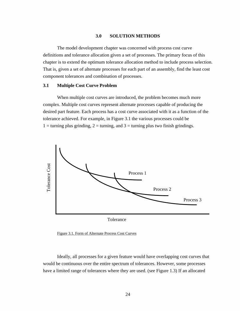
3.1 Multiple Cost Curve Problem

When multiple cost curves are introduced, the problem becomes much more

complex. Multiple cost curves represent alternate processes capable of producing the

desired part feature. Each process has a cost curve associated with it as a function of the

tolerance achieved. For example, in Figure 3.1 the various processes could be

1 = turning plus grinding, 2 = turning, and 3 = turning plus two finish grindings.

Process 3

Process 2

Process 1

Tol

eran

ce C

ost

Tolerance

Figure 3.1. Form of Alternate Process Cost Curves

Ideally, all processes for a given feature would have overlapping cost curves that

would be continuous over the entire spectrum of tolerances. However, some processes

have a limited range of tolerances where they are used. (see Figure 1.3) If an allocated

25

tolerance falls outside the feasible range of a process, another process must be chosen or

the tolerance must be fixed at the closest limiting value.

3.2 Experience with Branch and Bound

The OPTDES.BYU program contains a Branch and Bound algorithm to allow

discrete variable values to be included for analysis. Initially, a continuous optimum must

be found to specify the absolute optimum point available. For the process selection optimization, an iterative search technique is used which varies the exponent pi and the

cost coefficient Bi continuously until it finds an ideal cost curve for each part. The

permitted range of pi and Bi is set such that it includes all of the specified curves for each

part. The ideal optimum thus determined is then used as a comparison value from which

to start the discrete optimization problem. Various branches of the process tree are

evaluated to determine which branches could be eliminated (pruned) from the analysis.

The pruning is accomplished by taking one part at a time, substituting an actual process

curve, then performing a tolerance allocation and determining the assembly tolerance

cost. The selected process is held fixed while you move down that branch of the tree.

When you reach the end of the first branch, all of the ideal cost curves have been

replaced by specified process cost curves. The cost at that node is then used as a

temporary minimum for comparison with other combinations. Returning to the first part,

the next alternative process is selected and then evaluated by re-allocation. If it is not

lower in cost than the current minimum cost, the rest of that branch is eliminated from

consideration. This procedure is continued until every branch has either been evaluated or

eliminated.

The combination of continuous optimum tolerance allocation and discrete process

selection did not prove successful. The search surface became so bumpy or "noisy" due to

the re-allocation at each node that the search could not proceed to a global optimum

value. Many times the algorithm would find local minima and would not be able to go

any further. Sometimes it could not even find a feasible solution.

Even though the search method was unsuccessful in OPTDES, contour plots of

the assembly tolerance cost as a function of the curve parameters were generated in order

to examine the possible gradient patterns exhibited by the process selection problem. A

sample plot is shown in Figure 3.2 that shows cost contours for a general tolerance cost

function. The circle symbols represent actual processes. Note that the ideal process curve

always occurred in the lower right-hand corner. A little thought reveals this to be an

26

obvious result. The iterative search for the ideal curve was thus replaced by a simple scan of the range of pi and Bi.

-1.5

72.8

Process Cost Curve Exponent (p)

Proc

ess

Cos

t Cur

ve

Coe

ffic

ient

(B

)81.388.7 79.6 77.9 76.2 74.5

-1.4 -1.3 -1.2 -1.1 -1.0

0.0005

0.0010

0.0035

0.0030

0.0020

0.0015

0.0025

Optimum Point

= Discrete process cost c urve parameters

Figure 3.2. Assembly Tolerance Cost Contours

3.3 Exhaustive Search

The exhaustive search evaluates every possible process cost curve combination

and a tolerance allocation is computed for each one. It keeps track of the lowest cost

combination as it moves systematically through every node in the process tree The

number of combinations necessary for evaluation increases geometrically as the number of part processes increased. For an assembly with N parts, each parti having ni process

curves associated with it, the number of combinations was n1 x n2 x n3 x . . . x nN. For

example, an assembly with three parts that had 2, 2, and 3 curves for parts one, two and

three respectively would have 2 x 2 x 3 = 12 combinations to analyze in the exhaustive

search. An assembly that had ten parts with each part having just two process cost curves

per part would have 210 or 1024 combinations to check. The number of combinations

escalates rapidly for large numbers of parts and processes available. One test problem

with 13 parts and 38 process cost curves had over a million combinations. Figure 3.4

represents the possible combinations on the three part problem mentioned above and

27

depicted graphically in Figure 3.3 below. The cost figures are included for demonstration

purposes only. Note that after a process combination is selected, the tolerances must be

re-allocated and possibly have some adjustment of out-of-bound tolerances in order to

meet the assembly tolerance constraint. The noisy surface due to tolerance re-allocation

did not effect this method since all combinations were evaluated.

Tol

eran

ce C

ost

Tolerance

Process 3

Process 2

Process 1

Tol

eran

ce C

ost

Tolerance

Process 2

Process 1

Tol

eran

ce C

ost

Tolerance

Process 2

Process 1

Figure 3.3. Example Problem Process Cost Curves

28

Part 1

Part 2

Part 3

1

2

2

1

1

1

1

2

2

3

1

Assembly Cost

Trial Combinations

Alternate Processes

2

3

4

5

6

7

8

9

10

11

12

3

1

2

1

3

2

3

2

Minimum

$ 46.407

$ 43.336

$ 45.728

$ 49.916

$ 49.408

$ 44.397

$ 44.228

$ 41.008

$ 43.053

$ 49.102

$ 48.789

$ 42.685

Figure 3.4. Exhaustive Search Tree

3.4 Process Selection by Following the Lowest Curve Profile

Inspection of cost curve plots led to a search procedure in which the lowest cost

curves were chosen by a simple evaluation procedure. An initial combination of

processes was selected and the tolerances allocated. Then the alternate process cost

curves for the first part were compared for a lower cost at the same allocated tolerance

value. The lowest process cost curve for the given tolerance was then set as the current

29

process for that part. All parts were evaluated similarly by checking the available

processes for each part. If the entire part list was evaluated without any process curve

changes, then the process selection was considered complete. Otherwise a new allocation

was computed for the revised combination of processes and the evaluation procedure was

repeated.

Process 2

Process 1

Tol

eran

ce C

ost

Tolerance

Figure 3.5. Sample Process Cost Curve Switch

In other words, this method would follow the envelope or profile of the lowest

process cost curve values as the tolerances were allocated. If no other process cost curve

had a lower cost at the current tolerance allocation, the current process was not changed.

(see Figure 3.5) By searching the process tree with the tolerances fixed, the noisy surface

effects were greatly reduced. This method could always find a near optimum set of

tolerances with very few tolerance allocations. However, it did not consider any process

tolerance limits. For tolerance analysis cases with wide (essentially unconstrained)

process tolerance limits, this could be an efficient solution method.

3.5 Univariate Search with Tolerance Allocation

Through further examination of the exhaustive search trees similar to Figure 3.5

above, distinct assembly tolerance cost patterns were discovered. Because of the patterns

that developed in the original test cases, it was decided to use a univariate search to

determine the minimum assembly tolerance cost combination of processes. The concept

behind the univariate search is that the process tree has cost trends at the end of each tree

30

branch. Because of these trends, a simple search across each of the part levels can reveal

the best combination of processes to use. Each part would have its available processes

searched once, and the process that produced the lowest assembly tolerance cost was set

as the process for that part.

Figure 3.5 demonstrates how a univariate search is performed. First a set of

processes are selected, Lagrange multipliers are used to allocate the tolerances, and the

assembly tolerance cost is determined. In Figure 3.5, the starting processes are 1, 1, and

1. Then each of the part levels are searched. Part three has each of its alternate processes

selected, tolerances allocated, and cost determined. The minimum cost value on the first

part level search was with process 1 for part 3. Process 1 is then set for part 3, and the

search is continued on part 2. Process 2 for part 2 is selected and the assembly cost is

compared with the existing minimum cost. Process 1 for part 2 is set, and the search is

moved to part 1. Again, the alternate processes are checked, and process 2 for part 1 is set

as the better process. The final solution is processes 2, 1, 1 for parts 1, 2, 3 respectfully.

The univariate search required a minimal number of iterations before finding the

solution. The number of process combinations that had to be checked for a univariate

search was close to the sum of processes available. Specifically, for an assembly having N parts with ni process curves for parti, the number of combinations was

n1+n2+n3+...+nN.- N + 1. The problem depicted in Figure 3.3, an assembly having three

parts with 2,2, and 3 curves for parts one, two and three respectively, would have

2 + 2 + 3 - 3 + 1 = 5 combinations to check for the univariate search.

31

Part 1

Part 2

Part 3

1

2

2

1

1

1

1

2

2

3

1

Assembly Cost

Trial Combinations

Alternate Processes

2

3

4

5

3

1

2

1

3

2

3

2

Minimum

$ 43.336

$ 45.728

$ 49.408

$ 44.397

$ 41.008

Figure 3.6. Sample Tree for Univariate Search

Before stepping through the part levels of the process curve tree, however, a set of

processes that produced a valid or feasible starting case was necessary. Without a valid

starting set of processes, no cost comparisons could be made on initial process searches.

Therefore, two methods for determining a feasible starting point were developed. First,

two levels of the cost curve tree could be searched for a feasible point. Second, the

exhaustive search method could be started up until a feasible point was found. If the

32

exhaustive search was started, a tightly constrained problem may end up performing the

majority of the exhaustive search before a feasible starting point was found. However, it

was critical to the algorithm’s functionality that a feasible starting point be found. If none

was found, the algorithm could not be used.

For the majority of test cases, the univariate search found the absolute minimum

process combination. However, in some cases the univariate method was unable to find

the absolute minimum. If the process curves have upper tolerance range constraints, the

branch ends are not guaranteed to exhibit a uniform pattern. That means that there could

possibly be a large number of local minima throughout the design space. Only a lucky

starting place could produce the absolute minimum from the univariate search in such

cases Of most concern were process cost functions that had upper and lower tolerance

constraints and when process cost curves for the same parts had different exponents. In

general, a single univariate search can only guarantee a local minimum.

3.6 Continued Univariate Search

On many test cases, it was discovered that a univariate search would put the

solution in the vicinity of the global minimum. The univariate search could then be

started from the current univariate optimum and repeated until no better solution was

found. The stopping condition for the extended univariate search was met when no

process curves were changed during the search. If no process curves were changed, the

search could not proceed any further out of the current minimum point that it had found.

Like other general optimization techniques, a linear search is performed until a

minimum is found. Then a new search direction is determined and another search is

performed until a new search direction cannot be found that will improve on the objective

function.

This version of the univariate search was determined to be the best method next to

the exhaustive search. It matched the exhaustive search in accuracy in almost every case,

and it greatly deceased the number of process combinations tried. Noisy surface effects

due to tolerance re-allocation were the principle cause of inability to guarantee a global

minimum. Repeating the search nearly eliminated the problem.

A little hindsight revealed that the lowest curve-following method is really very

similar to the Univariate Search. Each part level is searched successively for the lowest

cost curve. However, the lowest curve-following method does not re-allocate tolerances

33

as it evaluates the curves. Re-allocation is performed only at the end of each univariate

search. This made the search surface more noisy and made the method less predictable.

3.7 Applying Tolerance Constraints by End-fixing

Manufacturing processes are generally only capable of producing parts over a

specified tolerance range. So an important factor in a valid process selection technique is

to ensure that the processes selected are compatible with the allocated tolerances. This

was accomplished by specifying the allowed tolerance range for each process. After

computing the optimum tolerance allocation for the selected set of processes for an

assembly, the resulting tolerances were checked to see if they were within the prescribed

range for each process. Those tolerances which were outside the limits were adjusted to

the nearest limit.

This "end-fixing" operation caused numerous problems. Whenever a component

tolerance was adjusted, the tolerance sum for the assembly was altered, so computation of

a new allocation was necessary, while holding the adjusted tolerance fixed. The new

allocation sometimes caused other tolerances to pop out-of-bounds, so the end-fixing and

re-allocating had to be repeated until no more out-of-bounds tolerances were created. The

procedure turned out to be highly order-dependent, giving completely different results

depending upon which tolerances were fixed first. It also could result in an infeasible

solution when all of the tolerances were fixed and the resulting sum violated the assembly

tolerance constraint.

The end-fixing also played havoc with the optimum process search methods. End-

fixing produced much greater search surface noise than tolerance re-allocation. None of

the search techniques performed well when end-fixing was necessary.

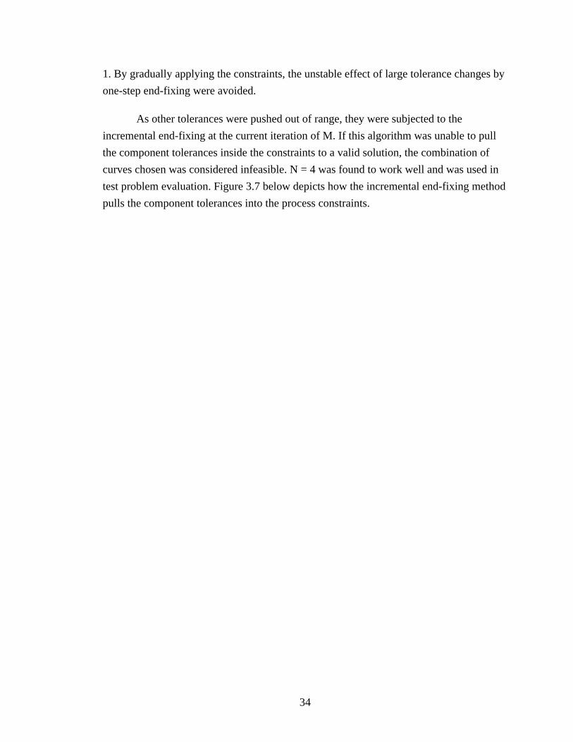
3.8 Incremental End-fixing

Fixing one out-of-bounds tolerance at a time was basically an unstable process. It

tended to cause large shifts in the tolerance allocations and unpredictable results. It was

decided that a method of gradually applying the tolerance constraints would be more

stable. The method for gradually applying the constraints consisted of repeating the

tolerance allocation for the selected set of processes by Lagrange multipliers N times and

fixing the out-of-range tolerances closer to the process tolerance constraints by steps. The

step length was set as the distance from the constraint divided by M as M went from N to

34

1. By gradually applying the constraints, the unstable effect of large tolerance changes by

one-step end-fixing were avoided.

As other tolerances were pushed out of range, they were subjected to the

incremental end-fixing at the current iteration of M. If this algorithm was unable to pull

the component tolerances inside the constraints to a valid solution, the combination of

curves chosen was considered infeasible. N = 4 was found to work well and was used in

test problem evaluation. Figure 3.7 below depicts how the incremental end-fixing method

pulls the component tolerances into the process constraints.

35

Part 1

Part 2

Part 3

Tolerance

Part 1

Part 2

Part 3

Tolerance

a) Start Incremental End-fixing with b) First Step: Additional Outlier Generated

one out-of-range tolerance (M = 4) (M = 3)

Part 1

Part 2

Part 3

Tolerance

Part 1

Part 2

Part 3

Tolerance

c) Second Step:Continue Constraint d) Third Step: One Step From Full Constraint

Application (M = 2) (M = 1)

Valid Tolerance Range

Out-of-Bounds Region

Current Part Tolerance Value

Figure 3.7. Incremental End-fixing

3.9 Process Search Performance with End-fixing

Each of the methods were modified to use the incremental end-fixing algorithm

(INC) and tested to see how they were affected by it. After the search algorithms selected

36

a set of processes cost curves, Lagrange multipliers were used to allocate the tolerances

and INC was used to assure that process tolerance constraints were met.

3.9.1 Exhaustive Search Method

When out-of-bound tolerances were fixed one at a time at process cost curve

limits, the solutions were not always the best available. Also, tightly constrained

problems would have a high number of combinations rejected as infeasible. By using

INC, the number of infeasible solutions decreased and the optimum costs decreased. Even

though the number of tolerance allocations often increased with INC, the increased

performance justified increased processing.

3.9.2 Bottom Curve Following Method

This method started with the unconstrained optimum cost solution and only dealt

with parts that had their allocated tolerances outside process tolerance constraints. As

with the exhaustive search method, the one-step end-fixing concept caused very

unpredictable results when tolerance constraints were applied, so INC was implemented

to stabilize the end-fixing variations. This method would select the initial set of process

cost curves, allocate the tolerances, and apply INC to make them conform to the

constraints. Then, it would step through the component tolerance list until it found a

tolerance that was fixed to meet the process tolerance constraints. If other processes were

available for that component, they were checked for a lower cost by setting each one as

the current process and re-allocating the tolerances using INC. If no other process cost

curves generated a lower assembly tolerance cost, the original curve was kept. If another

process cost curve produced a lower assembly tolerance cost, then the new curve was set

and the algorithm started through the tolerance list again.

By using INC the benefits of greater stability and a greater probability of finding a

global optimum were realized. This method also kept computing costs to a minimum by

only searching the part levels that had to be forced into process tolerance limits. Even

though this was a big improvement over the one-step end-fixing method, it was only able

to guarantee a local minimum.

3.9.3 Univariate Search Method

The univariate search is dependent on objective function patterns in order to find

the optimum value. With one-step end-fixing, the noisy surface would defeat the

37

univariate search sometimes by producing assembly tolerance costs that were not the least

cost for the set of process curves selected. However, by using INC, the noisy surface

effects were decreased. The assembly tolerance costs produced by INC for a given set of

process cost curves seemed to be the least cost set of tolerances with process tolerance

constraints applied. After implementing INC in the univariate search, it became almost as

accurate as the exhaustive search. The systematic searching of the univariate method

coupled with INC for tolerance allocation seemed to be the best combination next to the

exhaustive search and INC. Although you still could not guarantee the absolute minimum

assembly tolerance cost without running the exhaustive search.

38

4.0 RESULTS

In order to evaluate the performance of the various methods to find the best

process and tolerance combination for minimum assembly tolerance cost, some criteria

was set by which all methods were compared. The first comparison was on CPU time

needed to produce a solution. System timers were inserted in the computer code to

measure the CPU seconds used during an algorithm’s execution. Second, the number of

combinations tried was recorded to compare the effectiveness of the searching methods.

Third, the number of tolerance re-allocations was recorded in order to compare effects of

process tolerance ranges. And finally, the results from each method were compared with

the results from an exhaustive search. The exhaustive search was always able to find the

absolute minimum cost combination; it was used for the standard.

All methods described herein were evaluated on each of the test cases listed in the

appendix as well as other intermediate tests for numerical accuracy. Of the many

variations tried, it was determined that three methods would be evaluated in detail. The

three methods are listed below:

1) Exhaustive Search (EXH)

2) Bottom Curve Follower (BCF)

3) Extended Univariate Search (UNI)

4.1 Unconstrained Problems

The comparison on CPU time is depicted in Figure 4.1 for problems A through I.

The resolution of the system timer is 0.01 CPU seconds. For problems A to I, the

processes had no tolerance constraints and the exponents on the process cost curves were

all set at -1. This was done primarily to produce a uniform set of problems that would

compare CPU usage. Also, they correspond closely to the problem set used by Hauglund.

The unconstrained processes can, however, represent the general trends associated with

increased problem size.

39

0.01

0.1

1

10

100

1000

10000

100000

10 15 20 25 30 35 40

EXH

UNI

BCF

Number of Process Cost Curves

CPUSeconds

Figure 4.1. CPU Usage Comparison Chart

On problems A to I, each of the three methods evaluated arrived at the correct

solution to the problem. However, the CPU usage and number of process combinations

tried per problem varied greatly over the different methods. The performance criteria for

problems A to I is listed in Table 4.1 below.

Problem CPU Seconds Used Combinations Tried Tol. Re-allocations††

Name Size BCF UNI EXH BCF UNI EXH BCF UNI EXH

A 10 0.01 0.06 0.16 2 14 36 1 16 38

B 13 0.02 0.12 0.59 2 16 96 1 18 98

C 15 0.02 0.14 1.24 2 18 192 1 20 194

D 19 0.04 0.21 6.50 2 24 864 1 26 866

F 24 0.04 0.34 67.27 2 26 4096 1 28 4098

G 30 0.04 0.38 175.0 2 48 25600 1 50 25602

H 36 0.04 0.64 5388 2 50 531441 1 52 531443

I 38 0.04 0.73 11616 2 52 1062882 1 54 1062884 †† Numbers show all tolerance re-allocations including those from end-fixing

Table 4.1. Performance Values for Problems A-I

40

The results from the unbounded problems demonstrate the obvious differences in

CPU usage and number of combinations associated with the different methods. Although

each of the three methods arrived at the global minimum cost solution, BCF was the least

costly method for the unbounded problems. Obviously, EXH used up more CPU time

than the other methods, and it increased its CPU usage more rapidly than any of the other

methods as the size of the problems increased because all combinations had to be

checked. Ideal cases like problems A to I are useful for comparison of search algorithms

in unconstrained space, but another more complex set of test cases was necessary to

determine performance under more realistic condition in which various process tolerance

constraints are applied.

4.2 Problems with Process Constraints

The more complex set of test problems contained various process tolerance

constraints as well as having various process cost curve exponent values. For

demonstration purposes, three test problems were selected from numerous cases to

represent the general behavior of the test methods used. Each of the problems were

evaluated under three constraint conditions;

1) upper and lower process tolerance constraints,

2) only lower process tolerance constraints, and

3) unconstrained process tolerance constraints.

In addition to the process tolerance constraints, various combinations of process

cost curves were examined. The three problems are labeled T, U, and UU. Problem T had

all process cost curve exponents set at -2, problems U and UU had integer cost curve

exponents ranging from -1 to -3. The data for problem U was copied twice to create

problem UU, and the assembly tolerance for UU was set at twice that of problem U to

show the effects of problem size.

Figure 4.2 displays the CPU usage used in the various problems similar to Figure

4.1. Notice how the CPU time decreases as the constraints on the problem are relaxed.

41

0.001

0.01

0.1

1

10

T un U un UU un T low U low UU low T u/l U u/l UU u/l

BCF UNI EXH

Problem Name

CPUSeconds

Constraint conditions on processes: un = unbounded tolerance, low = lower tolerance bounds u/l = upper and lower tolerance bounds

Figure 4.2. CPU Usage for Problems T,U, and UU

The CPU usage is the time needed to return a solution for each of the problems, however,

sometimes only a local optimum was returned by the algorithms. In Table 4.2, the results

of the tests on problems T, U, and UU are displayed. Note that EXH was the only method

to guarantee the absolute minimum assembly tolerance cost in all cases.

42

Problem CPU Seconds Used Combinations Tried Tol. Re-allocations†† Name Size BCF UNI EXH BCF UNI EXH BCF UNI EXH

No Process Tolerance Constraints T 7 0.01 0.03 0.06 2 10 12 1 12 15 U 7 0.01* 0.07* 0.08 2 10 12 1 12 14 UU 14 0.02* 0.29 1.50 2 27 144 2 29 176

Only Lower Process Tolerance Constraints T 7 0.02 0.10 0.18 2 10 12 1 32 66 U 7 0.02 0.11 0.15 2 10 12 1 32 49 UU 14 0.04 0.51 4.66 2 18 144 2 75 811

Both Upper and Lower Process Tolerance Constraints T 7 0.06 0.16 0.15 4 10 12 16 57 76

U 7 0.07* 0.14* 0.14 3 10 12 27 62 74

UU 14 0.47 0.42 2.90 4 18 144 30 115 886 †† Numbers show all tolerance re-allocations including those from end-fixing * Found a local not global minimum

Table 4.2. Performance Data for Problems T,U, and UU

All three methods performed well when the special case of constant cost curve

exponents and only lower tolerance constraints were allowed. But the case of mixed cost

curve exponents and various tolerance constraints led to only near-minimum solutions.

Note that the CPU time does not increase appreciably with addition of constraints,

indicating the incremental end-fixing algorithm is efficient. Also, in the results for EXH,

the number of re-allocations is much higher than the number of combinations tried. This

indicates that a lot of end-fixing was necessary due to allocated tolerances which fell out

of the process tolerance ranges.

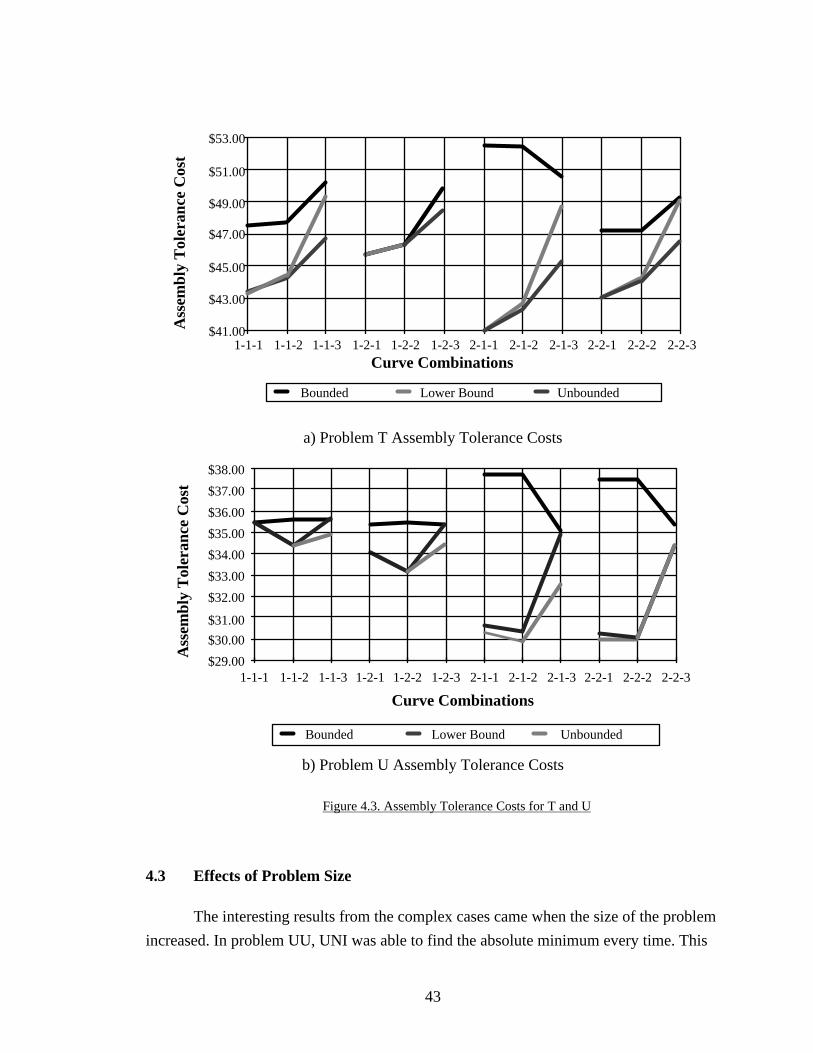
Figure 4.3 is a plot of assembly tolerance costs for all possible combinations of

problems T and U. This gives a feel for the nature of the discontinuous surface the

algorithms must search upon. It also shows the patterns of cost increase which occur as

the process is discretely varied for each part. The basic shape of the surface is greatly

changed when upper tolerance bounds are added. Repeating patterns are disturbed.

43

$41.00

$43.00

$45.00

$47.00

$49.00

$51.00

$53.00

Ass

embl

y T

oler

ance

Cos

t

Bounded Lower Bound Unbounded

1-1-1 1-1-2 1-1-3 1-2-1 1-2-2 1-2-3 2-1-1 2-1-2 2-1-3 2-2-1 2-2-2 2-2-3Curve Combinations

a) Problem T Assembly Tolerance Costs

Curve Combinations

1-1-1 1-1-2 1-1-3 1-2-1 1-2-2 1-2-3 2-1-1 2-1-2 2-1-3 2-2-1 2-2-2 2-2-3$29.00

$30.00

$31.00

$32.00

$33.00

$34.00

$35.00

$36.00

$37.00

$38.00

Ass

embl

y T

oler

ance

Cos

t

Bounded Lower Bound Unbounded

b) Problem U Assembly Tolerance Costs

Figure 4.3. Assembly Tolerance Costs for T and U

4.3 Effects of Problem Size

The interesting results from the complex cases came when the size of the problem

increased. In problem UU, UNI was able to find the absolute minimum every time. This

44

result is quite promising because EXH can be run on the smaller problems to guarantee a

minimum, and the larger problems that are too CPU intensive for EXH can use UNI. If

various starting points for UNI are chosen, the absolute minimum value is almost a

surety. It must be remembered, however, that the only way to guarantee the absolute

minimum assembly tolerance cost for all cases is to run EXH.

The complete numerical results for problems T, U, and UU can be found in

Appendix I. The appendix tables list the combinations and resulting costs for EXH. In

parallel columns, the search order of UNI is also included. Each UNI search is shown as a

separate column. Each UNI search starts at the minimum value of the previous search.

The absolute minimum is marked to show the desired answer. Note how UNI found the

optimum usually in two searches except for Problem U where it only found a local

minimum. The unconstrained process solution to UU did require three searches, but UNI

was still able to find the solution in a fraction of the time EXH needed. In some cases

identical minimum costs occur at more than one process combinations, then UNI finds

only one of them. The minimum found depends on the starting point of the search.

4.4 Limitations

The biggest concerns for cost optimization are 1) when alternate process cost

curves do not have overlapping tolerance ranges because of upper and lower tolerance

constraints, and 2) when process cost curves have different exponents. Both provide

complexities in themselves and multiply difficulties if combined.

If process cost curves have upper and lower tolerance constraints, the efficient

algorithms have no stable method of solution. All three of the solution methods return a

local minimum, but the absolute minimum is only guaranteed by EXH. Using only lower

tolerance constraints on the process cost curves did not cause significant problems and is

actually more true to life. Most manufacturing processes have limitations on the tightness

of their tolerances, but they are not limited on how rough they can go. Also, when the

tolerances get rougher, other less costly options become available and would provide a

lower process cost curve.

The mixed cost curve exponents were as difficult if not worse than the tolerance

constraints. However, UNI found the absolute minimum on almost all of the test

problems. If different starting points were chosen, UNI became even more likely to find

the solution.

45

Problem size had a big influence on the ability of the methods to find the absolute

minimum cost process combination. UNI had the most trouble with small size problems.

But if the problem was small, EXH was about the same cost as UNI and should be used.

When the problems got very large, UNI found the solution every time.

46

5.0 CONCLUSIONS AND RECOMMENDATIONS

5.1 Conclusions

The main conclusion from all tests performed is that EXH is the only method to

guarantee the global minimum assembly tolerance cost. The main problem associated

with the process selection was the noisy search surface. With multiple minima scattered

over the search surface, most methods will only find a local minimum and stay there.

That is why a global optimum is so difficult to guarantee when searching over a noisy

surface.

The decision on which method to use for analysis can be based on the number of

process combinations that exist in a problem. In general, EXH should be used when the

number of combinations is less than fifty. When the number of EXH combinations will

exceed fifty, UNI is recommended. Of course if the computing resources are unlimited,

EXH will guarantee the global optimum value for any problem.

Other factors may also be considered to influence the decision on which process

selection method to use.

1) Upper and lower process tolerance constraints used on process cost curves.

When this condition arises, the only guaranteed solution method is EXH.

However, if the number of EXH combinations will exceed fifty or the time

necessary for solution will exceed computer allocation time, then UNI should

be used.

2) Only lower process tolerance constraints are used on process cost curves.

Here UNI is recommended for all problems except for those with the number

of EXH combinations less than twenty or thirty. The exact cut-off point is

problem dependent and would require further study.

3) No process tolerance constraints are used on process cost curves.

When this condition exists, all methods in this thesis have a high probability

of returning the absolute minimum for the problem. The only restriction arises

when the process cost curve exponents are not the same. If the curve

exponents are the same for all processes connected to one part, but differ from

part to part, BCF, UNI or EXH can be used. If the process cost curve

exponents vary within the processes of one part, then EXH should be used

47

until the number of combinations exceed fifty, and then a UNI search is

recommended. However, if many tolerances need to be fixed for the solution,

the rules mentioned in (2) should be followed.

The limitations on using the methods other than EXH may raise some concerns

about the usefulness of the techniques presented here. However, the search surface

associated with the discrete process selection case can become something like a random

number field. The global minimum may be hidden amongst maximum extremes and/or

multitudes of local minima. If extreme conditions exist, extreme measures must be taken

to solve the problem. Therefore, EXH should always be available as an option.

5.2 Recommendations for Other Possible Methods

Although the methods presented herein are useful and can solve many complex

cases, they do not rule out other possibilities. A better method to solve the case where

upper and lower process tolerance constraints are applied may need to be developed.

Although the need for upper bounds has not been found from the limited data available,

some specialty applications may have circumstances that warrant such a method.

Exhaustive search times increase almost exponentially as the number of parts and

processes go up. Therefore, a method for locating the global minimum on a noisy surface,

while still maintaining the process tolerance constraints would be of great use.

5.2.1 Simulated Annealing Possibility

One documented method for solving multiple minima combinatorial problems is

the Simulated Annealing method. It is modelled after the ordering of atoms into a low-

energy state in a material as it is annealed.

Bohachevsky5 and Kirkpatrick6 along with others have demonstrated how

exhaustive searches are unnecessary for many large combinatorial problems if the

problems can be formulated into an annealing problem. The basic method randomly

perturbs the system parameters on a trial basis. If the objective function improves, the

perturbations are made permanent. If the objective function gets worse, it will still keep

the perturbations if there is a probability that by doing so it will eventually find an

extreme point better than the current one. This ability to jump out of local minima can

lead to the global minimum being found. However, it cannot guarantee the global

optimum. When the number of exhaustive search combinations becomes extremely large,

this may be a viable alternative. No references were discovered applying such an

48

algorithm to a process selection problem for tolerance analysis, but other combinatorial

examples tend to encourage further investigation.

5.2.2 Gradient Possibility

A major consideration for this problem was to use the Branch and Bound

algorithm in OPTDES.BYU to solve this type of problem with combined continuous and

discrete variables. However, the method used in OPTDES to deal with discrete solutions

was designed for a different type of problem than that needed for the specific problem of

multiple process cost curve analysis. Therefore, it was deemed inappropriate for the cost–

tolerance problem in its present form. However, the cost curve parameters were used in

OPTDES to generate a contour plot of the assembly tolerance cost contours as a function

of the cost curve parameters. (see Figure 3.2) If some general combined gradient method

could be developed to take advantage of the cost gradients and still account for tolerance

range limitations, it may prove successful in dealing with the exceptional cases that only

the exhaustive method has been able to solve reliably.

5.3 Need for Good Data

The main restriction on using any of the process selection methods is the need for

accurate process cost data. Once the data is established, analysis may begin. However,

exact costs for various processes may not be readily available in published form. Often it

is only available as a "rule of thumb" of some experienced manufacturing system analyst.

One project currently under way is the gathering of data at Garrett Turbine Engine

Co. on manufacturing costs. They determined that many parts have the processes

prescribed before manufacturing begins, but the number of cuts and type of cuts are not

determined until the part reaches the production floor. They are collecting data on similar

processes with rough and finish cuts coupled with grinding or finish processing. If

sufficient data can be gathered, it may be possible to break down a process into detailed

cost curves similar to Figure 5.1. Then the methods presented in this thesis could be used

to analyze the assembly and find the least cost solution.

49

1 R + 1 F + G

Tol

eran

ce C

ost

Tolerance

1 R + 2 F

1 R + 1 F

1 R

R = Rough Machine Cut F = Finish Machine Cut G = Grinding

Key

Figure 5.1. Example Combinations of Processes

By breaking down the processes performed into different operations, a

preliminary manufacturing process plan can be generated before the design leaves the

engineer’s hands. This is the type of communication that needs to be conveyed from the

shop floor to the engineering designers. When process costs and capabilities are known

during the design phases of a project, increased cost savings can and will be achieved.

5.4 CATS.BYU Recommendations

The tests performed in development of this thesis have demonstrated the

application of process selection in tolerance analysis and allocation. Because of the varied

nature in current tolerance analysis problems, this type of problem solving should be

included in the CATS.BYU program. This would bring increased capability for design

for manufacture to CATS. Although each of the methods described above have merit,

only the EXH and UNI methods are to be considered as useful and flexible methods for

process selection. Both EXH and UNI are therefore recommended to be implemented in

the CATS.BYU program. Because of the compact nature of BCF, it may also want to be

included for special cases, but it is not considered sufficiently flexible as a design method

to require implementation.

50

In order to provide a useful interface for implementation of these methods the

following suggestions are warranted.

5.4.1 Reference Handbook Data

As mentioned above, the most critical part of tolerance analysis is having accurate

data. Although engineers could look up cost data in reference tables or handbooks,

inclusion of cost curves for several standard processes as on-line data would enhance the

usefulness of process allocation techniques. Perhaps process curve data could be retrieved

through structured questions or on-screen selection of existing process models. Of course

the ability to enter user-specified cost data must be included, as should be the ability to

add and update data in the reference database.

Care should be taken as the methods for data retrieval are implemented with

concentration on presenting possibilities in a manner most acceptable to the user.

Processes could be selected by themselves, but the selection could be guided by type of

feature desired or type of material to be used or even by reference to what is most

commonly done in the shop by having a crude artificial intelligence for assistance.

5.4.2 Flexible Control Features

Besides flexible data access, other flexible features can enhance analysis

functionality and encourage greater use. Decisions on process selection methods may be

preset according to problem size and complexity. For example, if the number of

combinations is less than 20, the system would automatically use EXH. The user may

also want to analyze specific process combinations with and/or without process tolerance

constraints. Tolerance constraints might be turned on or off for analysis. An individual

process could be flagged as "fixed", turning off the search for alternate processes for a

specific part. And for the extreme cases, the user should be allowed to select a specific

combination of processes as a starting point for the process search. Another helpful

feature would keep track of the five lowest cost process combinations. Then if the user

wanted, they could decide between several good selections based on other considerations

than simply lowest cost. By including flexibility with CATS.BYU, its use as an

engineering design tool will increase and allow it to grow and change as as engineering

moves into the modern manufacturing era.

51

REFERENCES

Tolerance Analysis

1. Fortini, E. I., Dimensioning for Interchangeable Manufacture, Industrial Press, New York, 1967, p. 34-53

2. Chase and Greenwood, "Computer Aided Tolerance Selection: CATS.BYU User Guide", Mechanical Engineering Department, Brigham Young University, ADCATS Report No. 86–2, May 30, 1986

3. Greenwood, W.H., and Chase, K.W., "A New Tolerance Analysis Method for Designers and Manufacturers", Journal of Engineering for Industry, vol. 109, May 1987, p. 112-116

4. Greenwood, W.H., "A New Tolerance Analysis Method for Engineering Design and Manufacturing", Ph. D. Dissertation, Department of Mechanical Engineering, Brigham Young University, Provo, UT, 1987

Combinatorics

5. Bohachevsky, I. O., Johnson, M. E. , and Stein, M. L., "Generalized Simulated Annealing for Function Optimization", TECHNOMETRICS, Aug. 1986, Vol. 28,No. 3, p.209-217

6. Kirkpatrick, S., Gelatt, C. D., Vecchi, M. P.,"Optimization by Simulated Annealing", SCIENCE, Vol. 220, 13 May 1983, p. 671-680

7. Metropolis, N., Rosenbluth, A. W., Rosenbluth, M. N., and Teller, A. H., "Equation of State Calculations by Fast Computing Machines", The Journal of Chemical Physics, Vol. 21, No. 6, June 1953.

8. Hager, K., "A New Approach to Discrete Optimization of Steel Frames", Master's Thesis, Department of Civil Engineering, Brigham Young University, Provo, UT, 1987

9. Hauglund, L.F., "Combining Manufacturing Process Selection and Optimum Tolerance Allocation in Design Automation", Master's Thesis, Department of Mechanical Engineering, Brigham Young University, Provo, UT, 1987

Tolerance Optimization

10. Spotts, M.F., "Allocation of Tolerances to Minimize cost of Assembly", Journal of Engineering for Industry, August 1973, pp. 762–764

11. Ostwald, P.F., Huang, J., "A Method for Optimal Tolerance Selection", Journal of Engineering for Industry, Vol. 99, No. 3, Aug. 1977, p. 558-565.

52

12. Speckhart, F. H., "Calculation of Tolerance Based on a Minimum Cost Approach", Journal of Engineering for Industry, May 1972, p. 447-453.

13. Wilde, D., Prentice, E., "Minimum Exponential Cost Allocation of Sure-Fit Tolerances", Journal of Engineering for Industry, Nov. 1975, 1395-1398.

APPENDIX I

Data From Exhaustive and Extended Univariate Solutions

Problem A: Data and Solution ........... 53

53

Problem T: Exhaustive Search Iterations

(Univariate Search Iterations Listed)

Problem T Unbounded Problem T Lower Bounds Prob. T Upper & Lower Bounds

Exhaust. Asm. Tol. Curve Search Asm. Tol. Curve Search Asm. Tol. Curve SearchIteration Cost Comb. 1 2 Min Cost Comb. 1 2 Min Cost Comb. 1 2 Min

1 43.3364 1 1 1 1 5 43.3364 1 1 1 1 5 47.5672 1 1 1 1 42 44.2613 1 1 2 2 44.3970 1 1 2 2 47.7614 1 1 2 23 46.7066 1 1 3 3 49.4079 1 1 3 3 50.1881 1 1 3 34 45.7279 1 2 1 4 min 45.7279 1 2 1 4 45.7279 1 2 1 4 15 46.3753 1 2 2 46.4066 1 2 2 46.4066 1 2 2 26 48.4215 1 2 3 49.9158 1 2 3 49.9158 1 2 3 37 41.0082 2 1 1 5 1 41.0082 2 1 1 5 1 min 52.5071 2 1 1 8 42.3019 2 1 2 2 42.6849 2 1 2 2 52.4271 2 1 2 9 45.2759 2 1 3 3 48.7890 2 1 3 3 50.5144 2 1 3

10 43.0534 2 2 1 4 43.0534 2 2 1 4 47.2084 2 2 1 5 511 44.0522 2 2 2 44.2276 2 2 2 47.2078 2 2 2 12 46.6035 2 2 3 49.1018 2 2 3 49.3269 2 2 3

41.0082 Minimum Cost 41.0082 Minimum Cost 45.7279 Minimum Cost

Problem U: Exhaustive Search Iterations

(Univariate Search Iterations Listed)

Problem U Unbounded Problem U Lower Bounds Prob. U Upper & Lower Bounds

Exhaust. Asm. Tol. Curve Search Asm. Tol. Curve Search Asm. Tol. Curve SearchIteration Cost Comb. 1 2 Min Cost Comb. 1 2 Min Cost Comb. 1 2 Min

1 35.5269 1 1 1 1 35.5269 1 1 1 1 35.5269 1 1 1 1 42 34.3769 1 1 2 2 34.3769 1 1 2 2 35.6147 1 1 2 23 34.9061 1 1 3 3 35.6459 1 1 3 3 35.6459 1 1 3 34 34.1044 1 2 1 5 34.1044 1 2 1 35.3446 1 2 1 4 15 33.1808 1 2 2 4 33.1808 1 2 2 4 5 35.4918 1 2 2 26 34.4884 1 2 3 35.3808 1 2 3 35.3899 1 2 3 37 30.3059 2 1 1 4 30.6255 2 1 1 2 37.7348 2 1 18 29.8445 2 1 2 30.3617 2 1 2 4 37.7348 2 1 29 32.5651 2 1 3 34.9330 2 1 3 35.0931 2 1 3

10 29.9856 2 2 1 2 30.2420 2 2 1 37.4787 2 2 1 5 511 30.0522 2 2 2 5 1 30.0522 2 2 2 5 1 min 37.4787 2 2 212 34.3689 2 2 3 3 34.3746 2 2 3 3 35.3096 2 2 3

29.8445 Minimum Value 30.0522 Minimum Value 35.0931 Minimum Value

Problem A: Data and Solution ........... 54

54

Problem UU Without Tolerance Bounds: Exhaustive Search Iterations

(Univariate Search Iterations Listed)

Problem A: Data and Solution ........... 55

55

Problem UU Unbounded Problem UU Unbounded Problem UU UnboundedTol Process Curve Search Tol Process Curve Search Tol Process Curve Search

Iter Cost Combinations 1 2 3 Min Iter Cost Combinations 1 2 3 Min Iter. Cost Combinations 1 2 3 Min1 71.05 1 1 1 1 1 1 1 49 68.47 1 2 2 1 1 1 97 65.21 2 1 3 1 1 12 69.87 1 1 1 1 1 2 2 50 67.46 1 2 2 1 1 2 98 64.65 2 1 3 1 1 23 69.96 1 1 1 1 1 3 3 51 68.05 1 2 2 1 1 3 99 66.44 2 1 3 1 1 34 69.56 1 1 1 1 2 1 52 67.24 1 2 2 1 2 1 100 64.67 2 1 3 1 2 15 68.47 1 1 1 1 2 2 4 53 66.36 1 2 2 1 2 2 101 64.33 2 1 3 1 2 26 68.84 1 1 1 1 2 3 54 67.33 1 2 2 1 2 3 102 66.69 2 1 3 1 2 37 65.32 1 1 1 2 1 1 55 63.43 1 2 2 2 1 1 9 103 61.95 2 1 3 2 1 18 64.38 1 1 1 2 1 2 56 62.77 1 2 2 2 1 2 9 104 61.94 2 1 3 2 1 29 65.21 1 1 1 2 1 3 57 64.33 1 2 2 2 1 3 105 65.13 2 1 3 2 1 310 64.20 1 1 1 2 2 1 58 62.74 1 2 2 2 2 1 106 62.27 2 1 3 2 2 111 63.43 1 1 1 2 2 2 5 59 62.29 1 2 2 2 2 2 8 107 62.58 2 1 3 2 2 212 64.67 1 1 1 2 2 3 60 64.39 1 2 2 2 2 3 108 66.57 2 1 3 2 2 313 69.87 1 1 2 1 1 1 61 68.84 1 2 3 1 1 1 109 64.20 2 2 1 1 1 114 68.75 1 1 2 1 1 2 62 68.05 1 2 3 1 1 2 110 63.43 2 2 1 1 1 215 69.02 1 1 2 1 1 3 63 69.23 1 2 3 1 1 3 111 64.67 2 2 1 1 1 316 68.47 1 1 2 1 2 1 64 67.94 1 2 3 1 2 1 112 63.34 2 2 1 1 2 117 67.46 1 1 2 1 2 2 65 67.33 1 2 3 1 2 2 113 62.74 2 2 1 1 2 218 68.05 1 1 2 1 2 3 66 68.98 1 2 3 1 2 3 114 64.47 2 2 1 1 2 319 64.38 1 1 2 2 1 1 67 64.67 1 2 3 2 1 1 115 60.12 2 2 1 2 1 1 620 63.55 1 1 2 2 1 2 68 64.33 1 2 3 2 1 2 116 59.81 2 2 1 2 1 2 621 64.65 1 1 2 2 1 3 69 66.69 1 2 3 2 1 3 117 62.27 2 2 1 2 1 322 63.43 1 1 2 2 2 1 70 64.47 1 2 3 2 2 1 118 59.97 2 2 1 2 2 123 62.77 1 1 2 2 2 2 6 71 64.39 1 2 3 2 2 2 119 59.93 2 2 1 2 2 224 64.33 1 1 2 2 2 3 72 67.42 1 2 3 2 2 3 120 63.09 2 2 1 2 2 325 69.96 1 1 3 1 1 1 73 65.32 2 1 1 1 1 1 121 63.43 2 2 2 1 1 1 526 69.02 1 1 3 1 1 2 74 64.38 2 1 1 1 1 2 122 62.77 2 2 2 1 1 2 527 69.81 1 1 3 1 1 3 75 65.21 2 1 1 1 1 3 123 64.33 2 2 2 1 1 328 68.84 1 1 3 1 2 1 76 64.20 2 1 1 1 2 1 124 62.74 2 2 2 1 2 129 68.05 1 1 3 1 2 2 77 63.43 2 1 1 1 2 2 125 62.29 2 2 2 1 2 230 69.23 1 1 3 1 2 3 78 64.67 2 1 1 1 2 3 126 64.39 2 2 2 1 2 331 65.21 1 1 3 2 1 1 79 60.61 2 1 1 2 1 1 127 59.81 2 2 2 2 1 1 4 132 64.65 1 1 3 2 1 2 80 60.08 2 1 1 2 1 2 128 59.67 2 2 2 2 1 2 2 min33 66.44 1 1 3 2 1 3 81 61.95 2 1 1 2 1 3 129 62.58 2 2 2 2 1 3 334 64.67 1 1 3 2 2 1 82 60.12 2 1 1 2 2 1 130 59.93 2 2 2 2 2 1 235 64.33 1 1 3 2 2 2 7 83 59.81 2 1 1 2 2 2 131 60.10 2 2 2 2 2 2 9 1 436 66.69 1 1 3 2 2 3 84 62.27 2 1 1 2 2 3 132 63.79 2 2 2 2 2 3 337 69.56 1 2 1 1 1 1 85 64.38 2 1 2 1 1 1 133 64.67 2 2 3 1 1 138 68.47 1 2 1 1 1 2 86 63.55 2 1 2 1 1 2 134 64.33 2 2 3 1 1 239 68.84 1 2 1 1 1 3 87 64.65 2 1 2 1 1 3 135 66.69 2 2 3 1 1 340 68.21 1 2 1 1 2 1 88 63.43 2 1 2 1 2 1 136 64.47 2 2 3 1 2 141 67.24 1 2 1 1 2 2 89 62.77 2 1 2 1 2 2 137 64.39 2 2 3 1 2 242 67.94 1 2 1 1 2 3 90 64.33 2 1 2 1 2 3 138 67.42 2 2 3 1 2 343 64.20 1 2 1 2 1 1 91 60.08 2 1 2 2 1 1 8 139 62.27 2 2 3 2 1 1 744 63.43 1 2 1 2 1 2 92 59.69 2 1 2 2 1 2 8 140 62.58 2 2 3 2 1 2 745 64.67 1 2 1 2 1 3 93 61.94 2 1 2 2 1 3 141 66.57 2 2 3 2 1 346 63.34 1 2 1 2 2 1 94 59.81 2 1 2 2 2 1 142 63.09 2 2 3 2 2 147 62.74 1 2 1 2 2 2 95 59.67 2 1 2 2 2 2 min 143 63.79 2 2 3 2 2 248 64.47 1 2 1 2 2 3 96 62.58 2 1 2 2 2 3 144 68.74 2 2 3 2 2 3

Problem A: Data and Solution ........... 56

56

Problem UU With Only Lower Bounds: Exhaustive Search Iterations

(Univariate Search Iterations Listed)

Problem A: Data and Solution ........... 57

57

Problem UU Lower Bounds Problem UU Lower Bounds Problem UU Lower BoundsTol Process Curve Search Tol Process Curve Search Tol Process Curve Search

Iter Cost Combinations 1 2 Min Iter Cost Combinations 1 2 Min Iter. Cost Combinations 1 2 Min1 71.05 1 1 1 1 1 1 1 49 68.47 1 2 2 1 1 1 97 66.08 2 1 3 1 1 12 69.87 1 1 1 1 1 2 2 50 67.46 1 2 2 1 1 2 98 65.90 2 1 3 1 1 23 69.96 1 1 1 1 1 3 3 51 68.22 1 2 2 1 1 3 99 70.45 2 1 3 1 1 34 69.56 1 1 1 1 2 1 52 67.24 1 2 2 1 2 1 100 65.77 2 1 3 1 2 15 68.47 1 1 1 1 2 2 4 53 66.36 1 2 2 1 2 2 101 65.62 2 1 3 1 2 26 68.86 1 1 1 1 2 3 54 67.68 1 2 2 1 2 3 102 69.97 2 1 3 1 2 37 65.32 1 1 1 2 1 1 55 63.59 1 2 2 2 1 1 103 64.35 2 1 3 2 1 18 64.42 1 1 1 2 1 2 56 63.09 1 2 2 2 1 2 104 64.32 2 1 3 2 1 29 66.08 1 1 1 2 1 3 57 65.62 1 2 2 2 1 3 105 69.87 2 1 3 2 1 310 64.24 1 1 1 2 2 1 58 62.98 1 2 2 2 2 1 106 64.08 2 1 3 2 2 111 63.59 1 1 1 2 2 2 5 59 62.58 1 2 2 2 2 2 8 9 107 64.05 2 1 3 2 2 212 65.77 1 1 1 2 2 3 60 65.35 1 2 2 2 2 3 108 69.23 2 1 3 2 2 313 69.87 1 1 2 1 1 1 61 68.86 1 2 3 1 1 1 109 64.24 2 2 1 1 1 114 68.75 1 1 2 1 1 2 62 68.22 1 2 3 1 1 2 110 63.59 2 2 1 1 1 215 69.05 1 1 2 1 1 3 63 71.02 1 2 3 1 1 3 111 65.77 2 2 1 1 1 316 68.47 1 1 2 1 2 1 64 68.10 1 2 3 1 2 1 112 63.46 2 2 1 1 2 117 67.46 1 1 2 1 2 2 65 67.68 1 2 3 1 2 2 113 62.98 2 2 1 1 2 218 68.22 1 1 2 1 2 3 66 70.76 1 2 3 1 2 3 114 65.48 2 2 1 1 2 319 64.42 1 1 2 2 1 1 67 65.77 1 2 3 2 1 1 115 60.84 2 2 1 2 1 120 63.72 1 1 2 2 1 2 68 65.62 1 2 3 2 1 2 116 60.60 2 2 1 2 1 221 65.90 1 1 2 2 1 3 69 69.97 1 2 3 2 1 3 117 64.08 2 2 1 2 1 322 63.59 1 1 2 2 2 1 70 65.48 1 2 3 2 2 1 118 60.48 2 2 1 2 2 123 63.09 1 1 2 2 2 2 6 71 65.35 1 2 3 2 2 2 119 60.28 2 2 1 2 2 2 624 65.62 1 1 2 2 2 3 72 69.61 1 2 3 2 2 3 120 63.82 2 2 1 2 2 325 69.96 1 1 3 1 1 1 73 65.32 2 1 1 1 1 1 121 63.59 2 2 2 1 1 126 69.05 1 1 3 1 1 2 74 64.42 2 1 1 1 1 2 122 63.09 2 2 2 1 1 227 71.29 1 1 3 1 1 3 75 66.08 2 1 1 1 1 3 123 65.62 2 2 2 1 1 328 68.86 1 1 3 1 2 1 76 64.24 2 1 1 1 2 1 124 62.98 2 2 2 1 2 129 68.22 1 1 3 1 2 2 77 63.59 2 1 1 1 2 2 125 62.58 2 2 2 1 2 2 530 71.02 1 1 3 1 2 3 78 65.77 2 1 1 1 2 3 126 65.35 2 2 2 1 2 331 66.08 1 1 3 2 1 1 79 61.25 2 1 1 2 1 1 127 60.60 2 2 2 2 1 132 65.90 1 1 3 2 1 2 80 60.96 2 1 1 2 1 2 128 60.41 2 2 2 2 1 2 433 70.45 1 1 3 2 1 3 81 64.35 2 1 1 2 1 3 129 64.05 2 2 2 2 1 334 65.77 1 1 3 2 2 1 82 60.84 2 1 1 2 2 1 130 60.28 2 2 2 2 2 1 235 65.62 1 1 3 2 2 2 7 83 60.60 2 1 1 2 2 2 131 60.10 2 2 2 2 2 2 9 1 min36 69.97 1 1 3 2 2 3 84 64.08 2 1 1 2 2 3 132 63.79 2 2 2 2 2 3 337 69.56 1 2 1 1 1 1 85 64.42 2 1 2 1 1 1 133 65.77 2 2 3 1 1 138 68.47 1 2 1 1 1 2 86 63.72 2 1 2 1 1 2 134 65.62 2 2 3 1 1 239 68.86 1 2 1 1 1 3 87 65.90 2 1 2 1 1 3 135 69.97 2 2 3 1 1 340 68.21 1 2 1 1 2 1 88 63.59 2 1 2 1 2 1 136 65.48 2 2 3 1 2 141 67.24 1 2 1 1 2 2 89 63.09 2 1 2 1 2 2 137 65.35 2 2 3 1 2 242 68.10 1 2 1 1 2 3 90 65.62 2 1 2 1 2 3 138 69.61 2 2 3 1 2 343 64.24 1 2 1 2 1 1 91 60.96 2 1 2 2 1 1 139 64.08 2 2 3 2 1 144 63.59 1 2 1 2 1 2 92 60.72 2 1 2 2 1 2 140 64.05 2 2 3 2 1 245 65.77 1 2 1 2 1 3 93 64.32 2 1 2 2 1 3 141 69.23 2 2 3 2 1 346 63.46 1 2 1 2 2 1 94 60.60 2 1 2 2 2 1 142 63.82 2 2 3 2 2 147 62.98 1 2 1 2 2 2 95 60.41 2 1 2 2 2 2 8 143 63.79 2 2 3 2 2 2 748 65.48 1 2 1 2 2 3 96 64.05 2 1 2 2 2 3 144 68.75 2 2 3 2 2 3

Problem A: Data and Solution ........... 58

58

Problem UU With Upper and Lower Bounds: Exhaustive Search Iterations

(Univariate Search Iterations Listed)

Problem A: Data and Solution ........... 59

59

Prob UU Upper & Lower Bounds Prob UU Upper & Lower Bounds Prob UU Upper & Lower BoundsTol Process Curve Search Tol Process Curve Search Tol Process Curve Search

Iter Cost Combinations 1 2 Min Iter Cost Combinations 1 2 Min Iter. Cost Combinations 1 2 Min1 71.05 1 1 1 1 1 1 1 49 70.96 1 2 2 1 1 1 97 69.80 2 1 3 1 1 1 2 71.13 1 1 1 1 1 2 2 50 71.24 1 2 2 1 1 2 98 69.80 2 1 3 1 1 2 3 69.96 1 1 1 1 1 3 3 51 70.10 1 2 2 1 1 3 99 70.74 2 1 3 1 1 3 4 70.86 1 1 1 1 2 1 52 70.82 1 2 2 1 2 1 100 69.54 2 1 3 1 2 1 5 70.96 1 1 1 1 2 2 53 70.98 1 2 2 1 2 2 101 69.54 2 1 3 1 2 2 6 69.71 1 1 1 1 2 3 4 54 69.84 1 2 2 1 2 3 102 70.48 2 1 3 1 2 3 7 71.17 1 1 1 2 1 1 55 75.77 1 2 2 2 1 1 103 69.25 2 1 3 2 1 1 8 71.46 1 1 1 2 1 2 56 75.77 1 2 2 2 1 2 104 69.25 2 1 3 2 1 2 9 69.80 1 1 1 2 1 3 57 69.54 1 2 2 2 1 3 105 70.19 2 1 3 2 1 3 10 72.16 1 1 1 2 2 1 58 75.51 1 2 2 2 2 1 106 68.99 2 1 3 2 2 1 11 75.77 1 1 1 2 2 2 59 75.51 1 2 2 2 2 2 107 68.99 2 1 3 2 2 2 12 69.54 1 1 1 2 2 3 5 60 69.29 1 2 2 2 2 3 108 69.92 2 1 3 2 2 3 13 71.13 1 1 2 1 1 1 61 69.71 1 2 3 1 1 1 109 72.16 2 2 1 1 1 1 14 71.23 1 1 2 1 1 2 62 70.10 1 2 3 1 1 2 110 75.77 2 2 1 1 1 2 15 69.97 1 1 2 1 1 3 63 71.04 1 2 3 1 1 3 111 69.54 2 2 1 1 1 3 16 70.96 1 1 2 1 2 1 64 69.84 1 2 3 1 2 1 112 75.51 2 2 1 1 2 1 17 71.24 1 1 2 1 2 2 65 69.84 1 2 3 1 2 2 113 75.51 2 2 1 1 2 2 18 70.10 1 1 2 1 2 3 66 70.78 1 2 3 1 2 3 114 69.29 2 2 1 1 2 3 519 71.46 1 1 2 2 1 1 67 69.54 1 2 3 2 1 1 115 75.21 2 2 1 2 1 1 20 76.02 1 1 2 2 1 2 68 69.54 1 2 3 2 1 2 116 75.21 2 2 1 2 1 2 21 69.80 1 1 2 2 1 3 69 70.48 1 2 3 2 1 3 117 68.99 2 2 1 2 1 3 422 75.77 1 1 2 2 2 1 70 69.29 1 2 3 2 2 1 118 74.96 2 2 1 2 2 1 223 75.77 1 1 2 2 2 2 71 69.29 1 2 3 2 2 2 119 74.96 2 2 1 2 2 2 324 69.54 1 1 2 2 2 3 6 72 70.23 1 2 3 2 2 3 120 68.74 2 2 1 2 2 3 9 1 min25 69.96 1 1 3 1 1 1 73 71.17 2 1 1 1 1 1 121 75.77 2 2 2 1 1 1 26 69.97 1 1 3 1 1 2 74 71.46 2 1 1 1 1 2 122 75.77 2 2 2 1 1 2 27 71.29 1 1 3 1 1 3 75 69.80 2 1 1 1 1 3 123 69.54 2 2 2 1 1 3 28 69.71 1 1 3 1 2 1 76 72.16 2 1 1 1 2 1 124 75.51 2 2 2 1 2 1 29 70.10 1 1 3 1 2 2 77 75.77 2 1 1 1 2 2 125 75.51 2 2 2 1 2 2 30 71.04 1 1 3 1 2 3 78 69.54 2 1 1 1 2 3 126 69.29 2 2 2 1 2 3 31 69.80 1 1 3 2 1 1 79 75.47 2 1 1 2 1 1 127 75.21 2 2 2 2 1 1 32 69.80 1 1 3 2 1 2 80 75.47 2 1 1 2 1 2 128 75.21 2 2 2 2 1 2 33 70.74 1 1 3 2 1 3 81 69.25 2 1 1 2 1 3 129 68.99 2 2 2 2 1 3 34 69.54 1 1 3 2 2 1 82 75.21 2 1 1 2 2 1 130 74.96 2 2 2 2 2 1 35 69.54 1 1 3 2 2 2 83 75.21 2 1 1 2 2 2 131 74.96 2 2 2 2 2 2 36 70.48 1 1 3 2 2 3 7 84 68.99 2 1 1 2 2 3 8 132 68.74 2 2 2 2 2 3 6 min37 70.86 1 2 1 1 1 1 85 71.46 2 1 2 1 1 1 133 69.54 2 2 3 1 1 1 38 70.96 1 2 1 1 1 2 86 76.02 2 1 2 1 1 2 134 69.54 2 2 3 1 1 2 39 69.71 1 2 1 1 1 3 87 69.80 2 1 2 1 1 3 135 70.48 2 2 3 1 1 3 40 70.69 1 2 1 1 2 1 88 75.77 2 1 2 1 2 1 136 69.29 2 2 3 1 2 1 41 70.82 1 2 1 1 2 2 89 75.77 2 1 2 1 2 2 137 69.29 2 2 3 1 2 2 42 69.84 1 2 1 1 2 3 90 69.54 2 1 2 1 2 3 138 70.23 2 2 3 1 2 3 43 72.16 1 2 1 2 1 1 91 75.47 2 1 2 2 1 1 139 68.99 2 2 3 2 1 1 44 75.77 1 2 1 2 1 2 92 75.47 2 1 2 2 1 2 140 68.99 2 2 3 2 1 2 45 69.54 1 2 1 2 1 3 93 69.25 2 1 2 2 1 3 141 69.92 2 2 3 2 1 3 46 75.51 1 2 1 2 2 1 94 75.21 2 1 2 2 2 1 142 68.74 2 2 3 2 2 1 min47 75.51 1 2 1 2 2 2 95 75.21 2 1 2 2 2 2 143 68.74 2 2 3 2 2 2 min48 69.29 1 2 1 2 2 3 8 9 96 68.99 2 1 2 2 2 3 144 70.62 2 2 3 2 2 3 7

Problem A: Data and Solution ........... 60

60

0 12 24 36 48 60 72 84 96 108 120 132 14458

60

62

64

66

68

70

72Cost Data From UU Unbounded

Exhaustive Search Iteration

Ass

embl

y T

oler

ance

Cos

t

0 12 24 36 48 60 72 84 96 108 120 132 14460

62

64

66

68

70

72Cost Data From UU Lower Bounded

Exhaustive Search Iteration

Ass

embl

y T

oler

ance

Cos

t

Problem A: Data and Solution ........... 61

61

0 12 24 36 48 60 72 84 96 108 120 132 14468

70

72

74

76

78Cost Data From UU Upper & Lower Bounds

Exhaustive Search Iteration

Ass

embl

y T

oler

ance

Cos

t

Problem A: Data and Solution ........... 62

62

APPENDIX II

Listings of Sample Data Files and Their Solutions

Problem A: Data and Solution ........... 63

63

Problem A ____________________________________________________________________

Number of Curves: 10 Assembly Tolerance: 0.014 ____________________________________________________________________

Dimension Tolerance Fixed (1) CstMod RefTol RefCst FixCst Power MaxTol MinTol More ____________________________________________________________________

1.000000 0.35000000E-02 0 2 0.0010 6.0000 0.0000 -1.0000 0.0100 0.00050 1 2 0.0020 5.0000 0.0000 -1.0000 0.0100 0.00050 1 2 0.0050 2.0000 0.0000 -1.0000 0.0100 0.00050 0 1.000000 0.35000000E-02 0 2 0.0060 10.0000 0.0000 -1.0000 0.0100 0.00050 1 2 0.0080 8.0000 0.0000 -1.0000 0.0100 0.00050 0 1.000000 0.35000000E-02 0 2 0.0030 7.0000 0.0000 -1.0000 0.0100 0.00050 1 2 0.0040 5.0000 0.0000 -1.0000 0.0100 0.00050 0 1.000000 0.35000000E-02 0 2 0.0010 8.0000 0.0000 -1.0000 0.0100 0.00050 1 2 0.0020 5.0000 0.0000 -1.0000 0.0100 0.00050 1 2 0.0050 2.0000 0.0000 -1.0000 0.0100 0.00050 0

Solution Part Process Tolerance 1 1 0.0019600 2 1 0.0061982 3 2 0.0035785 4 1 0.0022633 Asm. Tolerance Cost 21.8650

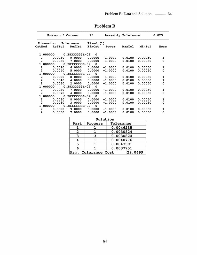
Problem B: Data and Solution ........... 64

64

Problem B ____________________________________________________________________

Number of Curves: 13 Assembly Tolerance: 0.023 ____________________________________________________________________

Dimension Tolerance Fixed (1) CstMod RefTol RefCst FixCst Power MaxTol MinTol More ____________________________________________________________________

1.000000 0.38333333E-02 0 2 0.0030 9.0000 0.0000 -1.0000 0.0100 0.00050 1 2 0.0050 7.0000 0.0000 -1.0000 0.0100 0.00050 0 1.000000 0.38333333E-02 0 2 0.0020 6.0000 0.0000 -1.0000 0.0100 0.00050 1 2 0.0040 5.0000 0.0000 -1.0000 0.0100 0.00050 0 1.000000 0.38333333E-02 0 2 0.0020 8.0000 0.0000 -1.0000 0.0100 0.00050 1 2 0.0040 4.0000 0.0000 -1.0000 0.0100 0.00050 1 2 0.0060 2.0000 0.0000 -1.0000 0.0100 0.00050 0 1.000000 0.38333333E-02 0 2 0.0030 7.0000 0.0000 -1.0000 0.0100 0.00050 1 2 0.0070 4.0000 0.0000 -1.0000 0.0100 0.00050 0 1.000000 0.38333333E-02 0 2 0.0030 8.0000 0.0000 -1.0000 0.0100 0.00050 1 2 0.0080 3.0000 0.0000 -1.0000 0.0100 0.00050 0 1.000000 0.38333333E-02 0 2 0.0020 9.0000 0.0000 -1.0000 0.0100 0.00050 1 2 0.0030 7.0000 0.0000 -1.0000 0.0100 0.00050 0

Solution Part Process Tolerance 1 1 0.0046235 2 1 0.0030824 3 3 0.0030824 4 1 0.0040776 5 1 0.0043591 6 1 0.0037751 Asm. Tolerance Cost 29.0499

Problem C: Data and Solution ........... 65

65

Problem C ____________________________________________________________________

Number of Curves: 15 Assembly Tolerance: 0.040 ____________________________________________________________________

Dimension Tolerance Fixed (1) CstMod RefTol RefCst FixCst Power MaxTol MinTol More ____________________________________________________________________

1.000000 0.57142857E-02 0 2 0.0010 9.0000 0.0000 -1.0000 0.0100 0.00050 1 2 0.0040 7.0000 0.0000 -1.0000 0.0100 0.00050 1 2 0.0060 6.0000 0.0000 -1.0000 0.0100 0.00050 0 1.000000 0.57142857E-02 0 2 0.0020 3.0000 0.0000 -1.0000 0.0100 0.00050 1 2 0.0040 2.0000 0.0000 -1.0000 0.0100 0.00050 0 1.000000 0.57142857E-02 0 2 0.0030 5.0000 0.0000 -1.0000 0.0100 0.00050 1 2 0.0040 4.0000 0.0000 -1.0000 0.0100 0.00050 0 1.000000 0.57142857E-02 0 2 0.0060 6.0000 0.0000 -1.0000 0.0100 0.00050 1 2 0.0080 4.0000 0.0000 -1.0000 0.0100 0.00050 0 1.000000 0.57142857E-02 0 2 0.0010 7.0000 0.0000 -1.0000 0.0100 0.00050 1 2 0.0050 2.0000 0.0000 -1.0000 0.0100 0.00050 0 1.000000 0.57142857E-02 0 2 0.0020 8.0000 0.0000 -1.0000 0.0100 0.00050 1 2 0.0040 5.0000 0.0000 -1.0000 0.0100 0.00050 0 1.000000 0.57142857E-02 0 2 0.0030 9.0000 0.0000 -1.0000 0.0100 0.00050 1 2 0.0070 8.0000 0.0000 -1.0000 0.0100 0.00050 0

Solution Part Process Tolerance 1 1 0.0044741 2 1 0.0036531 3 1 0.0057760 4 2 0.0084364 5 1 0.0039458 6 1 0.0059654 7 1 0.0077493 Asm. Tolerance Cost 17.9845

Problem D: Data and Solution ........... 66

66

Problem D ____________________________________________________________________

Number of Curves: 19 Assembly Tolerance: 0.033 ____________________________________________________________________

Dimension Tolerance Fixed (1) CstMod RefTol RefCst FixCst Power MaxTol MinTol More ____________________________________________________________________

1.000000 0.41250000E-02 0 2 0.0010 6.0000 0.0000 -1.0000 0.0100 0.00050 1 2 0.0040 4.0000 0.0000 -1.0000 0.0100 0.00050 0 1.000000 0.41250000E-02 0 2 0.0020 8.0000 0.0000 -1.0000 0.0100 0.00050 1 2 0.0040 6.0000 0.0000 -1.0000 0.0100 0.00050 0 1.000000 0.41250000E-02 0 2 0.0060 5.0000 0.0000 -1.0000 0.0100 0.00050 1 2 0.0080 4.0000 0.0000 -1.0000 0.0100 0.00050 1 2 0.0090 2.0000 0.0000 -1.0000 0.0100 0.00050 0 1.000000 0.41250000E-02 0 2 0.0030 6.0000 0.0000 -1.0000 0.0100 0.00050 1 2 0.0050 4.0000 0.0000 -1.0000 0.0100 0.00050 0 1.000000 0.41250000E-02 0 2 0.0020 8.0000 0.0000 -1.0000 0.0100 0.00050 1 2 0.0050 7.0000 0.0000 -1.0000 0.0100 0.00050 1 2 0.0070 2.0000 0.0000 -1.0000 0.0100 0.00050 0 1.000000 0.41250000E-02 0 2 0.0030 6.0000 0.0000 -1.0000 0.0100 0.00050 1 2 0.0040 3.0000 0.0000 -1.0000 0.0100 0.00050 0 1.000000 0.41250000E-02 0 2 0.0050 9.0000 0.0000 -1.0000 0.0100 0.00050 1 2 0.0070 7.0000 0.0000 -1.0000 0.0100 0.00050 0 1.000000 0.41250000E-02 0 2 0.0010 9.0000 0.0000 -1.0000 0.0100 0.00050 1 2 0.0030 6.0000 0.0000 -1.0000 0.0100 0.00050 1 2 0.0040 1.0000 0.0000 -1.0000 0.0100 0.00050 0

Solution Part Process Tolerance 1 1 0.0026203 2 1 0.0042789 3 3 0.0045385 4 1 0.0045385 5 3 0.0040026 6 2 0.0037057 7 1 0.0071760 8 3 0.0021395 Asm. Tolerance Cost 28.8377

Problem F: Data and Solution ............ 67

67

Problem F ____________________________________________________________________

Number of Curves: 24 Assembly Tolerance: 0.040 ____________________________________________________________________

Dimension Tolerance Fixed (1) CstMod RefTol RefCst FixCst Power MaxTol MinTol More ____________________________________________________________________

1.000000 0.33333333E-02 0 2 0.0010 10.0000 0.0000 -1.0000 0.0100 0.00050 1 2 0.0030 7.0000 0.0000 -1.0000 0.0100 0.00050 0 1.000000 0.33333333E-02 0 2 0.0030 7.0000 0.0000 -1.0000 0.0100 0.00050 1 2 0.0050 5.0000 0.0000 -1.0000 0.0100 0.00050 0 1.000000 0.33333333E-02 0 2 0.0020 5.0000 0.0000 -1.0000 0.0100 0.00050 1 2 0.0040 3.0000 0.0000 -1.0000 0.0100 0.00050 0 1.000000 0.33333333E-02 0 2 0.0060 3.0000 0.0000 -1.0000 0.0100 0.00050 1 2 0.0070 1.0000 0.0000 -1.0000 0.0100 0.00050 0 1.000000 0.33333333E-02 0 2 0.0020 12.0000 0.0000 -1.0000 0.0100 0.00050 1 2 0.0050 6.0000 0.0000 -1.0000 0.0100 0.00050 0 1.000000 0.33333333E-02 0 2 0.0010 10.0000 0.0000 -1.0000 0.0100 0.00050 1 2 0.0030 7.0000 0.0000 -1.0000 0.0100 0.00050 0 1.000000 0.33333333E-02 0 2 0.0060 9.0000 0.0000 -1.0000 0.0100 0.00050 1 2 0.0070 7.0000 0.0000 -1.0000 0.0100 0.00050 0 1.000000 0.33333333E-02 0 2 0.0010 9.0000 0.0000 -1.0000 0.0100 0.00050 1 2 0.0040 8.0000 0.0000 -1.0000 0.0100 0.00050 0 1.000000 0.33333333E-02 0 2 0.0030 10.0000 0.0000 -1.0000 0.0100 0.00050 1 2 0.0050 9.0000 0.0000 -1.0000 0.0100 0.00050 0 1.000000 0.33333333E-02 0 2 0.0010 15.0000 0.0000 -1.0000 0.0100 0.00050 1 2 0.0020 14.0000 0.0000 -1.0000 0.0100 0.00050 0 1.000000 0.33333333E-02 0 2 0.0030 20.0000 0.0000 -1.0000 0.0100 0.00050 1 2 0.0040 15.0000 0.0000 -1.0000 0.0100 0.00050 0 1.000000 0.33333333E-02 0 2 0.0010 10.0000 0.0000 -1.0000 0.0100 0.00050 1 2 0.0050 5.0000 0.0000 -1.0000 0.0100 0.00050 0

Problem F: Data and Solution ............ 68

68

Solution Part Process Tolerance 1 1 0.0024385 2 1 0.0035337 3 1 0.0024385 4 2 0.0020402 5 1 0.0037777 6 1 0.0024385 7 2 0.0053978 8 1 0.0023134 9 1 0.0042236 10 1 0.0029865 11 1 0.0059731 12 1 0.0024385 Asm. Tolerance Cost 67.2691

Problem G: Data and Solution ........... 69

69

Problem G ____________________________________________________________________

Number of Curves: 30 Assembly Tolerance: 0.035 ____________________________________________________________________

Dimension Tolerance Fixed (1) CstMod RefTol RefCst FixCst Power MaxTol MinTol More ____________________________________________________________________

1.000000 0.50000000E-02 0 2 0.0020 10.0000 0.0000 -1.0000 0.0100 0.00050 1 2 0.0030 7.0000 0.0000 -1.0000 0.0100 0.00050 1 2 0.0040 6.0000 0.0000 -1.0000 0.0100 0.00050 1 2 0.0050 5.0000 0.0000 -1.0000 0.0100 0.00050 1 2 0.0070 3.0000 0.0000 -1.0000 0.0100 0.00050 0 1.000000 0.50000000E-02 0 2 0.0020 12.0000 0.0000 -1.0000 0.0100 0.00050 1 2 0.0040 8.0000 0.0000 -1.0000 0.0100 0.00050 1 2 0.0060 7.0000 0.0000 -1.0000 0.0100 0.00050 1 2 0.0080 4.0000 0.0000 -1.0000 0.0100 0.00050 1 2 0.0100 2.0000 0.0000 -1.0000 0.0100 0.00050 0 1.000000 0.50000000E-02 0 2 0.0030 9.0000 0.0000 -1.0000 0.0100 0.00050 1 2 0.0040 8.0000 0.0000 -1.0000 0.0100 0.00050 1 2 0.0060 6.0000 0.0000 -1.0000 0.0100 0.00050 1 2 0.0080 5.0000 0.0000 -1.0000 0.0100 0.00050 0 1.000000 0.50000000E-02 0 2 0.0010 14.0000 0.0000 -1.0000 0.0100 0.00050 1 2 0.0030 12.0000 0.0000 -1.0000 0.0100 0.00050 1 2 0.0040 10.0000 0.0000 -1.0000 0.0100 0.00050 1 2 0.0060 9.0000 0.0000 -1.0000 0.0100 0.00050 0 1.000000 0.50000000E-02 0 2 0.0020 20.0000 0.0000 -1.0000 0.0100 0.00050 1 2 0.0030 19.0000 0.0000 -1.0000 0.0100 0.00050 1 2 0.0040 17.0000 0.0000 -1.0000 0.0100 0.00050 1 2 0.0070 12.0000 0.0000 -1.0000 0.0100 0.00050 0 1.000000 0.50000000E-02 0 2 0.0030 4.0000 0.0000 -1.0000 0.0100 0.00050 1 2 0.0040 3.0000 0.0000 -1.0000 0.0100 0.00050 1 2 0.0050 2.0000 0.0000 -1.0000 0.0100 0.00050 1 2 0.0060 1.0000 0.0000 -1.0000 0.0100 0.00050 0 1.000000 0.50000000E-02 0 2 0.0030 10.0000 0.0000 -1.0000 0.0100 0.00050 1 2 0.0040 8.0000 0.0000 -1.0000 0.0100 0.00050 1 2 0.0070 7.0000 0.0000 -1.0000 0.0100 0.00050 1 2 0.0090 4.0000 0.0000 -1.0000 0.0100 0.00050 0

Solution Part Process Tolerance 1 1 0.0048711 2 5 0.0048711 3 1 0.0056597 4 1 0.0040755 5 1 0.0068888 6 4 0.0026680 7 1 0.0059659 Asm. Tolerance Cost 29.5015

Problem H: Data and Solution ........... 70

70

Problem H ____________________________________________________________________

Number of Curves: 36 Assembly Tolerance: 0.036 ____________________________________________________________________

Dimension Tolerance Fixed (1) CstMod RefTol RefCst FixCst Power MaxTol MinTol More ____________________________________________________________________

1.000000 0.30000000E-02 0 2 0.0010 10.0000 0.0000 -1.0000 0.0100 0.00050 1 2 0.0020 9.0000 0.0000 -1.0000 0.0100 0.00050 1 2 0.0030 8.0000 0.0000 -1.0000 0.0100 0.00050 0 1.000000 0.30000000E-02 0 2 0.0010 9.0000 0.0000 -1.0000 0.0100 0.00050 1 2 0.0040 7.0000 0.0000 -1.0000 0.0100 0.00050 1 2 0.0050 6.0000 0.0000 -1.0000 0.0100 0.00050 0 1.000000 0.30000000E-02 0 2 0.0020 8.0000 0.0000 -1.0000 0.0100 0.00050 1 2 0.0040 7.0000 0.0000 -1.0000 0.0100 0.00050 1 2 0.0060 4.0000 0.0000 -1.0000 0.0100 0.00050 0 1.000000 0.30000000E-02 0 2 0.0030 7.0000 0.0000 -1.0000 0.0100 0.00050 1 2 0.0040 4.0000 0.0000 -1.0000 0.0100 0.00050 1 2 0.0050 2.0000 0.0000 -1.0000 0.0100 0.00050 0 1.000000 0.30000000E-02 0 2 0.0010 10.0000 0.0000 -1.0000 0.0100 0.00050 1 2 0.0040 5.0000 0.0000 -1.0000 0.0100 0.00050 1 2 0.0050 2.0000 0.0000 -1.0000 0.0100 0.00050 0 1.000000 0.30000000E-02 0 2 0.0010 6.0000 0.0000 -1.0000 0.0100 0.00050 1 2 0.0020 4.0000 0.0000 -1.0000 0.0100 0.00050 1 2 0.0030 3.0000 0.0000 -1.0000 0.0100 0.00050 0 1.000000 0.30000000E-02 0 2 0.0020 7.0000 0.0000 -1.0000 0.0100 0.00050 1 2 0.0030 6.0000 0.0000 -1.0000 0.0100 0.00050 1 2 0.0060 5.0000 0.0000 -1.0000 0.0100 0.00050 0 1.000000 0.30000000E-02 0 2 0.0040 10.0000 0.0000 -1.0000 0.0100 0.00050 1 2 0.0060 9.0000 0.0000 -1.0000 0.0100 0.00050 1 2 0.0080 8.0000 0.0000 -1.0000 0.0100 0.00050 0 1.000000 0.30000000E-02 0 2 0.0010 10.0000 0.0000 -1.0000 0.0100 0.00050 1 2 0.0040 7.0000 0.0000 -1.0000 0.0100 0.00050 1 2 0.0050 6.0000 0.0000 -1.0000 0.0100 0.00050 0 1.000000 0.30000000E-02 0 2 0.0020 9.0000 0.0000 -1.0000 0.0100 0.00050 1 2 0.0040 6.0000 0.0000 -1.0000 0.0100 0.00050 1 2 0.0050 3.0000 0.0000 -1.0000 0.0100 0.00050 0 1.000000 0.30000000E-02 0 2 0.0030 8.0000 0.0000 -1.0000 0.0100 0.00050 1 2 0.0060 7.0000 0.0000 -1.0000 0.0100 0.00050 1 2 0.0080 6.0000 0.0000 -1.0000 0.0100 0.00050 0 1.000000 0.30000000E-02 0 2 0.0010 9.0000 0.0000 -1.0000 0.0100 0.00050 1 2 0.0020 7.0000 0.0000 -1.0000 0.0100 0.00050 1 2 0.0040 6.0000 0.0000 -1.0000 0.0100 0.00050 0

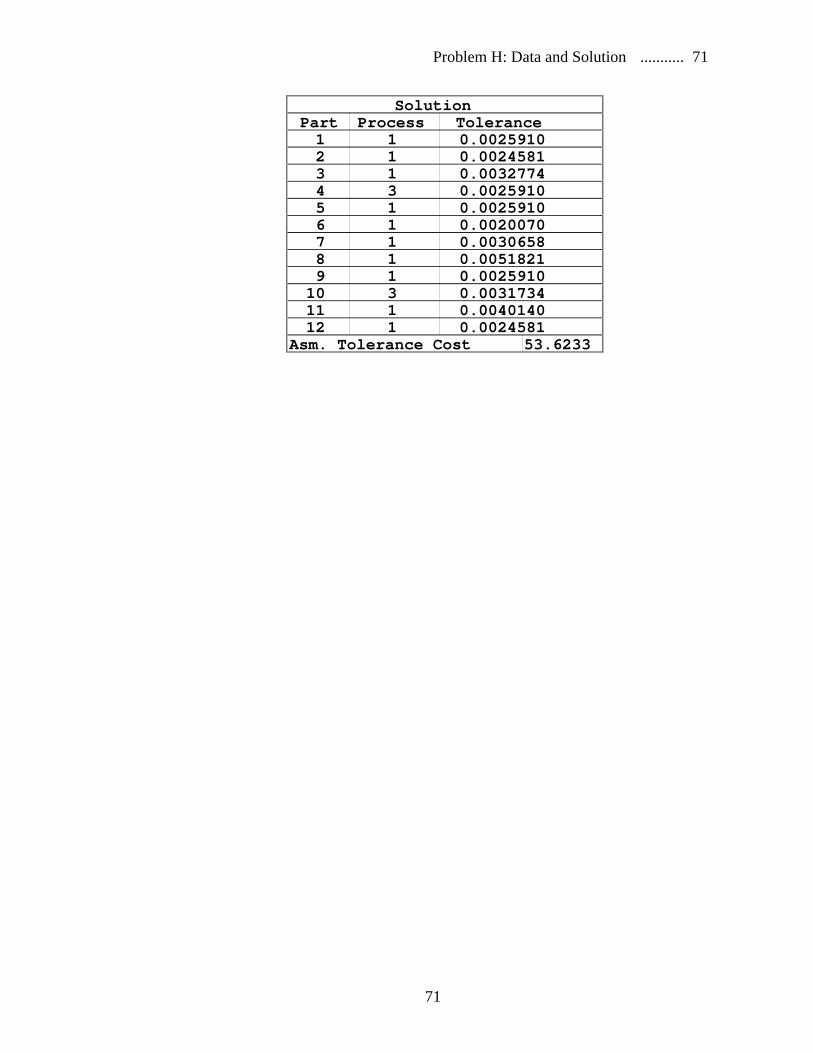
Problem H: Data and Solution ........... 71

71

Solution Part Process Tolerance 1 1 0.0025910 2 1 0.0024581 3 1 0.0032774 4 3 0.0025910 5 1 0.0025910 6 1 0.0020070 7 1 0.0030658 8 1 0.0051821 9 1 0.0025910 10 3 0.0031734 11 1 0.0040140 12 1 0.0024581 Asm. Tolerance Cost 53.6233

Problem T Process Cost Curves ......... 72

72

Problem I ____________________________________________________________________

Number of Curves: 38 Assembly Tolerance: 0.036 ____________________________________________________________________

Dimension Tolerance Fixed (1) CstMod RefTol RefCst FixCst Power MaxTol MinTol More ____________________________________________________________________

1.000000 0.27692308E-02 0 2 0.0010 10.0000 0.0000 -1.0000 0.0100 0.00050 1 2 0.0020 9.0000 0.0000 -1.0000 0.0100 0.00050 1 2 0.0030 8.0000 0.0000 -1.0000 0.0100 0.00050 0 1.000000 0.27692308E-02 0 2 0.0010 9.0000 0.0000 -1.0000 0.0100 0.00050 1 2 0.0040 7.0000 0.0000 -1.0000 0.0100 0.00050 1 2 0.0050 6.0000 0.0000 -1.0000 0.0100 0.00050 0 1.000000 0.27692308E-02 0 2 0.0020 8.0000 0.0000 -1.0000 0.0100 0.00050 1 2 0.0040 7.0000 0.0000 -1.0000 0.0100 0.00050 1 2 0.0060 4.0000 0.0000 -1.0000 0.0100 0.00050 0 1.000000 0.27692308E-02 0 2 0.0030 7.0000 0.0000 -1.0000 0.0100 0.00050 1 2 0.0040 4.0000 0.0000 -1.0000 0.0100 0.00050 1 2 0.0050 2.0000 0.0000 -1.0000 0.0100 0.00050 0 1.000000 0.27692308E-02 0 2 0.0010 10.0000 0.0000 -1.0000 0.0100 0.00050 1 2 0.0040 5.0000 0.0000 -1.0000 0.0100 0.00050 1 2 0.0050 2.0000 0.0000 -1.0000 0.0100 0.00050 0 1.000000 0.27692308E-02 0 2 0.0010 6.0000 0.0000 -1.0000 0.0100 0.00050 1 2 0.0020 4.0000 0.0000 -1.0000 0.0100 0.00050 1 2 0.0030 3.0000 0.0000 -1.0000 0.0100 0.00050 0 1.000000 0.27692308E-02 0 2 0.0020 7.0000 0.0000 -1.0000 0.0100 0.00050 1 2 0.0030 6.0000 0.0000 -1.0000 0.0100 0.00050 1 2 0.0060 5.0000 0.0000 -1.0000 0.0100 0.00050 0 1.000000 0.27692308E-02 0 2 0.0040 10.0000 0.0000 -1.0000 0.0100 0.00050 1 2 0.0060 9.0000 0.0000 -1.0000 0.0100 0.00050 1 2 0.0080 8.0000 0.0000 -1.0000 0.0100 0.00050 0 1.000000 0.27692308E-02 0 2 0.0010 10.0000 0.0000 -1.0000 0.0100 0.00050 1 2 0.0040 7.0000 0.0000 -1.0000 0.0100 0.00050 1 2 0.0050 6.0000 0.0000 -1.0000 0.0100 0.00050 0 1.000000 0.27692308E-02 0 2 0.0020 9.0000 0.0000 -1.0000 0.0100 0.00050 1 2 0.0040 6.0000 0.0000 -1.0000 0.0100 0.00050 1 2 0.0050 3.0000 0.0000 -1.0000 0.0100 0.00050 0 1.000000 0.27692308E-02 0 2 0.0030 8.0000 0.0000 -1.0000 0.0100 0.00050 1 2 0.0060 7.0000 0.0000 -1.0000 0.0100 0.00050 1 2 0.0080 6.0000 0.0000 -1.0000 0.0100 0.00050 0 1.000000 0.27692308E-02 0 2 0.0010 9.0000 0.0000 -1.0000 0.0100 0.00050 1 2 0.0020 7.0000 0.0000 -1.0000 0.0100 0.00050 1 2 0.0040 6.0000 0.0000 -1.0000 0.0100 0.00050 0

Problem T Process Cost Curves ......... 73

73

1.000000 0.27692308E-02 0 2 0.0010 8.0000 0.0000 -1.0000 0.0100 0.00050 1 2 0.0020 3.0000 0.0000 -1.0000 0.0100 0.00050 0

Solution Part Process Tolerance 1 1 0.0024542 2 1 0.0023283 3 1 0.0031044 4 3 0.0024542 5 1 0.0024542 6 1 0.0019010 7 1 0.0029039 8 1 0.0049084 9 1 0.0024542 10 3 0.0030058 11 1 0.0038021 12 1 0.0023283 13 2 0.0019010 Asm. Tolerance Cost 59.7690

Problem T Process Cost Curves ......... 74

74

Tol

eran

ce C

ost

10

15

20

25

30

35

40

45

0.0035 0.0045 0.0055 0.0065Tolerance

Process 1 = 2 =

Problem T: Processes for Part 1

10

20

30

40

50

60

70

0.0015 0.0025 0.0035 0.0045Tolerance

Tol

eran

ce C

ost Process

1 = 2 =

Problem T: Processes for Part 2

Tol

eran

ce C

ost

8

10

12

14

16

18

20

22

0.0019 0.0031 0.0043 0.0055Tolerance

Process 1 = 2 = 3 =

Problem T: Processes for Part 3

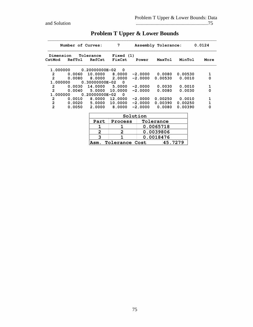
Problem T Upper & Lower Bounds: Data and Solution ..........................................................75

75

Problem T Upper & Lower Bounds ____________________________________________________________________

Number of Curves: 7 Assembly Tolerance: 0.0124 ____________________________________________________________________

Dimension Tolerance Fixed (1) CstMod RefTol RefCst FixCst Power MaxTol MinTol More ____________________________________________________________________

1.000000 0.20000000E-02 0 2 0.0060 10.0000 8.0000 -2.0000 0.0080 0.00530 1 2 0.0080 8.0000 2.0000 -2.0000 0.00530 0.0010 0 1.000000 0.30000000E-02 0 2 0.0030 14.0000 5.0000 -2.0000 0.0030 0.0010 1 2 0.0040 5.0000 10.0000 -2.0000 0.0080 0.0030 0 1.000000 0.20000000E-02 0 2 0.0010 8.0000 12.0000 -2.0000 0.00250 0.0010 1 2 0.0020 5.0000 10.0000 -2.0000 0.00390 0.00250 1 2 0.0050 2.0000 8.0000 -2.0000 0.0080 0.00390 0

Solution Part Process Tolerance 1 1 0.0065718 2 2 0.0039806 3 1 0.0018476 Asm. Tolerance Cost 45.7279

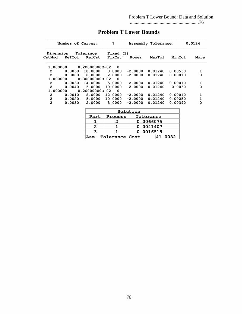
Problem T Lower Bound: Data and Solution ..........................................................76

76

Problem T Lower Bounds ____________________________________________________________________

Number of Curves: 7 Assembly Tolerance: 0.0124 ____________________________________________________________________

Dimension Tolerance Fixed (1) CstMod RefTol RefCst FixCst Power MaxTol MinTol More ____________________________________________________________________

1.000000 0.20000000E-02 0 2 0.0060 10.0000 8.0000 -2.0000 0.01240 0.00530 1 2 0.0080 8.0000 2.0000 -2.0000 0.01240 0.00010 0 1.000000 0.30000000E-02 0 2 0.0030 14.0000 5.0000 -2.0000 0.01240 0.00010 1 2 0.0040 5.0000 10.0000 -2.0000 0.01240 0.0030 0 1.000000 0.20000000E-02 0 2 0.0010 8.0000 12.0000 -2.0000 0.01240 0.00010 1 2 0.0020 5.0000 10.0000 -2.0000 0.01240 0.00250 1 2 0.0050 2.0000 8.0000 -2.0000 0.01240 0.00390 0

Solution Part Process Tolerance 1 2 0.0066075 2 1 0.0041407 3 1 0.0016519 Asm. Tolerance Cost 41.0082

Problem T Unbounded: Data and Solution 77

77

Problem T Unbounded ____________________________________________________________________

Number of Curves: 7 Assembly Tolerance: 0.0124 ____________________________________________________________________

Dimension Tolerance Fixed (1) CstMod RefTol RefCst FixCst Power MaxTol MinTol More ____________________________________________________________________

1.000000 0.20000000E-02 0 2 0.0060 10.0000 8.0000 -2.0000 0.01240 0.00010 1 2 0.0080 8.0000 2.0000 -2.0000 0.01240 0.00010 0 1.000000 0.30000000E-02 0 2 0.0030 14.0000 5.0000 -2.0000 0.01240 0.00010 1 2 0.0040 5.0000 10.0000 -2.0000 0.01240 0.00010 0 1.000000 0.20000000E-02 0 2 0.0010 8.0000 12.0000 -2.0000 0.01240 0.00010 1 2 0.0020 5.0000 10.0000 -2.0000 0.01240 0.00010 1 2 0.0050 2.0000 8.0000 -2.0000 0.01240 0.00010 0

Solution Part Process Tolerance 1 2 0.0066075 2 1 0.0041407 3 1 0.0016519 Asm. Tolerance Cost 41.0082

Problem U Process Cost Curves ........ 78

78

0

5

10

15

20

25

30

35

40

45

0.0035 0.0045 0.0055 0.0065Tolerance

Tol

eran

ce C

ost Process

1 = 2 =

Problem U: Processes for Part 1

0

24

6

8

10

12

14

16

18

20

0.002 0.003 0.004 0.005Tolerance

Tol

eran

ce C

ost Process

1 = 2 =

Problem U: Processes for Part 2

5

7

9

11

13

15

17

19

0.0015 0.0027 0.0039 0.0051Tolerance

Process 1 = 2 = 3 =

Tol

eran

ce C

ost

Problem U Process Cost Curves ........ 79

79

Problem U: Processes for Part 3

Problem U Upper & Lower Bounds: Data and Solution ..........................................................80

80

Problem U Upper & Lower Bounds ____________________________________________________________________

Number of Curves: 7 Assembly Tolerance: 0.0124 ____________________________________________________________________

Dimension Tolerance Fixed (1) CstMod RefTol RefCst FixCst Power MaxTol MinTol More ____________________________________________________________________

1.000000 0.20000000E-02 0 2 0.0060 10.0000 7.0000 -1.0000 0.0080 0.00540 1 2 0.0080 8.0000 0.0000 -2.0000 0.00540 0.0010 0 1.000000 0.30000000E-02 0 2 0.0030 7.0000 1.0000 -1.0000 0.0080 0.00340 1 2 0.0040 5.0000 0.0000 -2.0000 0.00340 0.0010 0 1.000000 0.20000000E-02 0 2 0.0010 8.0000 9.0000 -1.0000 0.00350 0.0020 1 2 0.0020 5.0000 8.0000 -2.0000 0.0020 0.0010 1 2 0.0050 2.0000 5.0000 -3.0000 0.0080 0.00350 0

Solution Part Process Tolerance 1 2 0.0054000 fix 2 1 0.0034000 fix 3 3 0.0036000 Asm. Tolerance Cost 35.0931

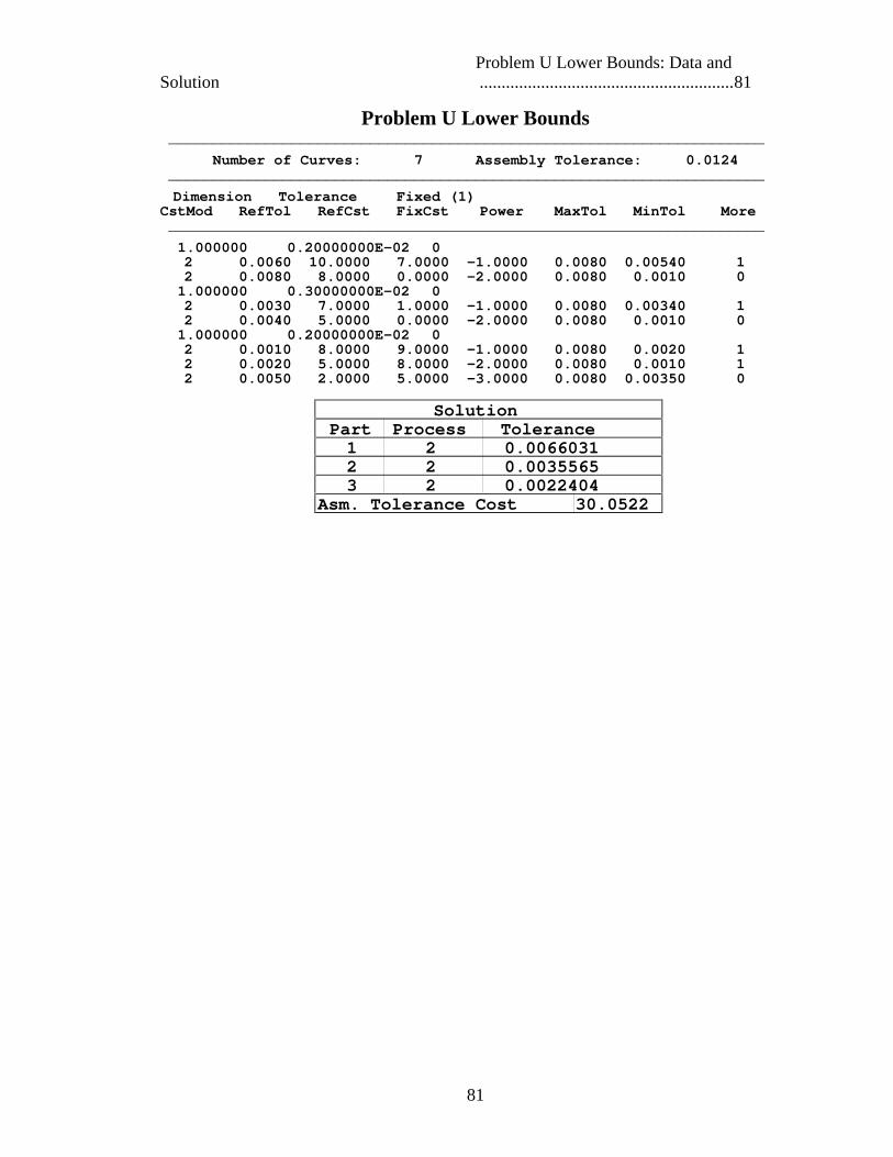
Problem U Lower Bounds: Data and Solution ..........................................................81

81

Problem U Lower Bounds ____________________________________________________________________

Number of Curves: 7 Assembly Tolerance: 0.0124 ____________________________________________________________________

Dimension Tolerance Fixed (1) CstMod RefTol RefCst FixCst Power MaxTol MinTol More ____________________________________________________________________

1.000000 0.20000000E-02 0 2 0.0060 10.0000 7.0000 -1.0000 0.0080 0.00540 1 2 0.0080 8.0000 0.0000 -2.0000 0.0080 0.0010 0 1.000000 0.30000000E-02 0 2 0.0030 7.0000 1.0000 -1.0000 0.0080 0.00340 1 2 0.0040 5.0000 0.0000 -2.0000 0.0080 0.0010 0 1.000000 0.20000000E-02 0 2 0.0010 8.0000 9.0000 -1.0000 0.0080 0.0020 1 2 0.0020 5.0000 8.0000 -2.0000 0.0080 0.0010 1 2 0.0050 2.0000 5.0000 -3.0000 0.0080 0.00350 0

Solution Part Process Tolerance 1 2 0.0066031 2 2 0.0035565 3 2 0.0022404 Asm. Tolerance Cost 30.0522

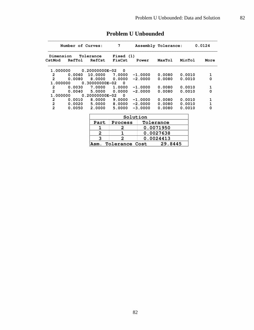
Problem U Unbounded: Data and Solution 82

82

Problem U Unbounded ____________________________________________________________________

Number of Curves: 7 Assembly Tolerance: 0.0124 ____________________________________________________________________

Dimension Tolerance Fixed (1) CstMod RefTol RefCst FixCst Power MaxTol MinTol More ____________________________________________________________________

1.000000 0.20000000E-02 0 2 0.0060 10.0000 7.0000 -1.0000 0.0080 0.0010 1 2 0.0080 8.0000 0.0000 -2.0000 0.0080 0.0010 0 1.000000 0.30000000E-02 0 2 0.0030 7.0000 1.0000 -1.0000 0.0080 0.0010 1 2 0.0040 5.0000 0.0000 -2.0000 0.0080 0.0010 0 1.000000 0.20000000E-02 0 2 0.0010 8.0000 9.0000 -1.0000 0.0080 0.0010 1 2 0.0020 5.0000 8.0000 -2.0000 0.0080 0.0010 1 2 0.0050 2.0000 5.0000 -3.0000 0.0080 0.0010 0

Solution Part Process Tolerance 1 2 0.0071950 2 1 0.0027638 3 2 0.0024413 Asm. Tolerance Cost 29.8445

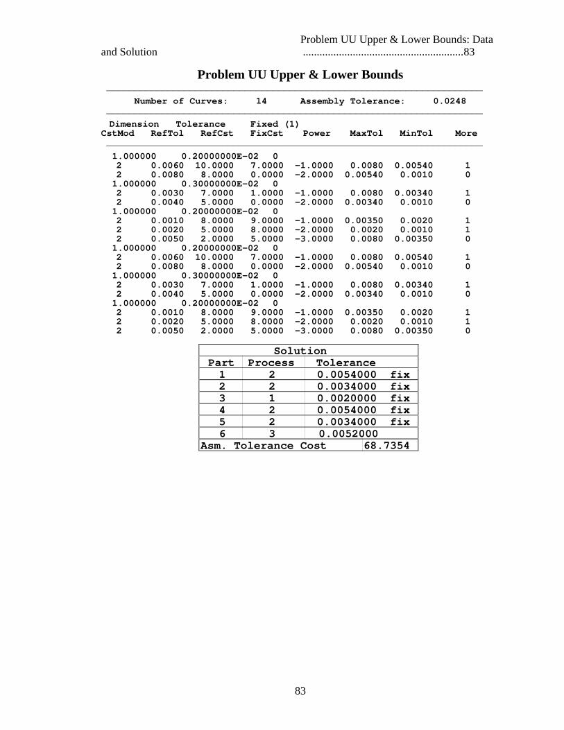
Problem UU Upper & Lower Bounds: Data and Solution ..........................................................83

83

Problem UU Upper & Lower Bounds ____________________________________________________________________

Number of Curves: 14 Assembly Tolerance: 0.0248 ____________________________________________________________________

Dimension Tolerance Fixed (1) CstMod RefTol RefCst FixCst Power MaxTol MinTol More ____________________________________________________________________

1.000000 0.20000000E-02 0 2 0.0060 10.0000 7.0000 -1.0000 0.0080 0.00540 1 2 0.0080 8.0000 0.0000 -2.0000 0.00540 0.0010 0 1.000000 0.30000000E-02 0 2 0.0030 7.0000 1.0000 -1.0000 0.0080 0.00340 1 2 0.0040 5.0000 0.0000 -2.0000 0.00340 0.0010 0 1.000000 0.20000000E-02 0 2 0.0010 8.0000 9.0000 -1.0000 0.00350 0.0020 1 2 0.0020 5.0000 8.0000 -2.0000 0.0020 0.0010 1 2 0.0050 2.0000 5.0000 -3.0000 0.0080 0.00350 0 1.000000 0.20000000E-02 0 2 0.0060 10.0000 7.0000 -1.0000 0.0080 0.00540 1 2 0.0080 8.0000 0.0000 -2.0000 0.00540 0.0010 0 1.000000 0.30000000E-02 0 2 0.0030 7.0000 1.0000 -1.0000 0.0080 0.00340 1 2 0.0040 5.0000 0.0000 -2.0000 0.00340 0.0010 0 1.000000 0.20000000E-02 0 2 0.0010 8.0000 9.0000 -1.0000 0.00350 0.0020 1 2 0.0020 5.0000 8.0000 -2.0000 0.0020 0.0010 1 2 0.0050 2.0000 5.0000 -3.0000 0.0080 0.00350 0

Solution Part Process Tolerance 1 2 0.0054000 fix 2 2 0.0034000 fix 3 1 0.0020000 fix 4 2 0.0054000 fix 5 2 0.0034000 fix 6 3 0.0052000 Asm. Tolerance Cost 68.7354

Problem UU Lower Bounds: Data and Solution ..........................................................84

84

Problem UU Lower Bounds ____________________________________________________________________

Number of Curves: 14 Assembly Tolerance: 0.0248 ____________________________________________________________________

Dimension Tolerance Fixed (1) CstMod RefTol RefCst FixCst Power MaxTol MinTol More ____________________________________________________________________

1.000000 0.20000000E-02 0 2 0.0060 10.0000 7.0000 -1.0000 0.0080 0.00540 1 2 0.0080 8.0000 0.0000 -2.0000 0.0080 0.0010 0 1.000000 0.30000000E-02 0 2 0.0030 7.0000 1.0000 -1.0000 0.0080 0.00340 1 2 0.0040 5.0000 0.0000 -2.0000 0.0080 0.0010 0 1.000000 0.20000000E-02 0 2 0.0010 8.0000 9.0000 -1.0000 0.0080 0.0020 1 2 0.0020 5.0000 8.0000 -2.0000 0.0080 0.0010 1 2 0.0050 2.0000 5.0000 -3.0000 0.0080 0.00350 0 1.000000 0.20000000E-02 0 2 0.0060 10.0000 7.0000 -1.0000 0.0080 0.00540 1 2 0.0080 8.0000 0.0000 -2.0000 0.0080 0.0010 0 1.000000 0.30000000E-02 0 2 0.0030 7.0000 1.0000 -1.0000 0.0080 0.00340 1 2 0.0040 5.0000 0.0000 -2.0000 0.0080 0.0010 0 1.000000 0.20000000E-02 0 2 0.0010 8.0000 9.0000 -1.0000 0.0080 0.0020 1 2 0.0020 5.0000 8.0000 -2.0000 0.0080 0.0010 1 2 0.0050 2.0000 5.0000 -3.0000 0.0080 0.00350 0

Solution Part Process Tolerance 1 2 0.0066031 2 2 0.0035565 3 2 0.0022404 4 2 0.0066031 5 2 0.0035565 6 2 0.0022404 Asm. Tolerance Cost 60.1044

Problem UU Lower Bounds: Data and Solution ..........................................................85

85

Problem UU Unbounded ____________________________________________________________________

Number of Curves: 14 Assembly Tolerance: 0.0248 ____________________________________________________________________

Dimension Tolerance Fixed (1) CstMod RefTol RefCst FixCst Power MaxTol MinTol More ____________________________________________________________________

1.000000 0.20000000E-02 0 2 0.0060 10.0000 7.0000 -1.0000 0.0080 0.0010 1 2 0.0080 8.0000 0.0000 -2.0000 0.0080 0.0010 0 1.000000 0.30000000E-02 0 2 0.0030 7.0000 1.0000 -1.0000 0.0080 0.0010 1 2 0.0040 5.0000 0.0000 -2.0000 0.0080 0.0010 0 1.000000 0.20000000E-02 0 2 0.0010 8.0000 9.0000 -1.0000 0.0080 0.0010 1 2 0.0020 5.0000 8.0000 -2.0000 0.0080 0.0010 1 2 0.0050 2.0000 5.0000 -3.0000 0.0080 0.0010 0 1.000000 0.20000000E-02 0 2 0.0060 10.0000 7.0000 -1.0000 0.0080 0.0010 1 2 0.0080 8.0000 0.0000 -2.0000 0.0080 0.0010 0 1.000000 0.30000000E-02 0 2 0.0030 7.0000 1.0000 -1.0000 0.0080 0.0010 1 2 0.0040 5.0000 0.0000 -2.0000 0.0080 0.0010 0 1.000000 0.20000000E-02 0 2 0.0010 8.0000 9.0000 -1.0000 0.0080 0.0010 1 2 0.0020 5.0000 8.0000 -2.0000 0.0080 0.0010 1 2 0.0050 2.0000 5.0000 -3.0000 0.0080 0.0010 0

Solution Part Process Tolerance 1 2 0.0069015 2 1 0.0025964 3 2 0.0023417 4 2 0.0069015 5 2 0.0037172 6 2 0.0023417 Asm. Tolerance Cost 59.6711