manufacturing transition in local economies: a regional
TRANSCRIPT
Manufacturing Transition in Local Economies:
A Regional Adjustment Model1
Jason P. Brown1,† Dayton M. Lambert2, and Raymond J.G.M. Florax3,4
1 USDA, Economic Research Service
1800 M St. NW, Washington, D.C. 20036–5831 E-mail: [email protected]
2 Dept. of Agricultural and Resource Economics, University of Tennessee
2621 Morgan Hall, Knoxville, Tennessee 37996–4518 E-mail: [email protected]
3 Dept. of Agricultural Economics, Purdue University 403 W. State Street, West Lafayette, IN 47907–2056
E-mail: [email protected]
4 Dept. of Spatial Economics, VU University Amsterdam De Boelelaan 1105, 1081 HV Amsterdam, The Netherlands
Selected Paper prepared for presentation at the Agricultural & Applied Economics Association 2010 AAEA, CAES & WAEA Joint Annual Meeting, Denver, Colorado, July 25-27, 2010
1 The views expressed here are those of the authors, and may not be attributed to the Economic Research Service, the U.S. Department of Agriculture, the University of Tennessee, or Purdue University. † Corresponding author.
1
Manufacturing Transition in Local Economies: A Regional Adjustment Model
Abstract This paper addresses changes in capital formation by testing the importance of location factors with respect to the rate of establishment births and deaths in U.S. manufacturing, 2000–2004. A theoretical concept called “localized creative destruction” is tested as a mechanism to explain the dynamics impacting the spatial distribution of manufacturing establishment birth and death rates. While no support of this process was found, results identify a convergence process occurring where counties with high initial birth/death rates have smaller changes in firm birth and death rates. The interpretation is that counties become more equally competitive in terms of firm formation dynamics in lieu of successful counties increasing their lead in the short run. This is potentially relevant to policymakers and economic development practitioners who are concerned with business retention and the impact of new manufacturing establishments on their existing base. Key words: location determinants, manufacturing, adjustment models JEL Codes: L60, R11, R12 1. INTRODUCTION
The United States economy has experienced four recessions since the 1980s, including the most
recent one which began in the fourth quarter of 2007. Over the same period, but especially in the
1990’s, rural areas in the United States struggled as manufacturing investment flowed back to
urban areas, drawn by better access to skilled labor, business services, and product and input
markets. The impact of this trend was magnified by the 2001 recession, when rural areas in
particular suffered from this spatial realignment because of their higher relative shares of
manufacturing employment as compared to metropolitan areas (WILKERSON, 2001). Increased
global integration of product markets has also heightened competition in domestic
manufacturing, eroding the competitive advantage of rural areas once typified by lower labor
costs (MCGRANAHAN, 2002). The spatial concentration of manufacturing investment in urban
areas has also increased because of the growing importance of a skilled workforce, supply-chain
logistics, and lower costs arising from (external) scale economies. These events have translated

2
into changes in the capital stock of manufacturing as well as in the spatial distribution of capital
stock. While the causality of these events is difficult to untangle, changes in technology sets used
in production as well as changes in product markets constitute important drivers of reallocation
trends.
Research documents that technological and industrial renewal occurs through a
simultaneous process of micro-evolutionary changes in technology and discontinuous
technological innovations (BAUM, 1996). As Schumpeter observed, technological innovation
and technology adoption may also be driven by birth (market entry) and death (exit) of
manufacturing establishments via a process of “creative destruction” (SCHUMPETER, 1942, p.
83).2 The extent to which exiting firms are replaced by new establishments is also influenced by
local and regional economic and demographic determinants. The industrial organization
literature documents many examples of firm behavior with respect to entry-exit dynamics even
within narrowly defined industries (BARTELSMAN et al., 2003). Firms continuously enter and
exit markets. Among entering firms, many fail to survive during the first few years, while others
prosper. Even during good times, the number of firms in a sector may decrease, while in other
locations or sectors firm recruitment increases. Consequently, changes in employment following
plant opening and closing are as important as changes due to firm expansion or contraction of
surviving firms (HAMERMESH, 1993). These dynamics may have important implications for
local business attraction and retention strategies pursued by policymakers.
2 The terms “entry” and “exit” are synonymous with birth and death in the theoretical and empirical industrial organization literature (HOPENHAYM, 1992; ERICSON and PAKES, 1995; PAKES and ERICSON, 1998; BALDWIN and GORECKI, 1991; JOHNSON and PARKER, 1996; REYNOLDS et al., 1995; LOVE, 1996; FOTOPOULOS and SPENCE, 1998). Our convention is that the dynamic process of establishment birth and may be viewed as creative destruction.
3
This paper investigates the relative importance of location determinants related to birth
and death of manufacturing establishments in the U.S., during the time period 2000–2004.
Although the spatial and temporal dynamics of birth and death processes are obviously related,
the causal direction is difficult to discern as birth/death occurs simultaneously. Establishment
birth and death are therefore hypothesized to be endogenous. In addition, the possibility of a
heterogeneous response to location factors impacting birth and death across space cannot be
ruled out a priori. This paper follows PE’ER and VERTINSKY (2008) testing for a localized
process of creative destruction, in a novel way allowing for spatial spillovers between counties.
Simultaneously allowing for spatial heterogeneity and localized spillovers provides a richer
context for explaining the spatial distribution of manufacturing establishment birth and death.
Understanding why firms choose specific locations and the resulting spatial and temporal
dynamics driving firm birth and death may help policymakers better understand the process of
regional growth and renewal. This information is useful in light of economic development
policies designed to attract or retain manufacturing investment (MALECKI, 2004; HART, 2008).
2. BACKGROUND
An obvious and very pervasive empirical regularity occurring in the study of birth and
death rates of establishments is their high correlation (DUNNE et al., 1988; CABLE and
SCHWALBACH, 1991; BRUCE et al., 2007; BOSMA et al., 2008). Schumpeter’s theory of
creative destruction is often cited to motivate and explain this general phenomenon. Schumpeter
maintained that the vitality of an economic engine in a capitalist society depends on the
formation of new goods and services, new methods of production or transportation, new forms of
industrial organization, and new product and input markets. Schumpeter emphasized that firm
4
formation by entrepreneurs is crucial for revolutionizing “… the pattern of production by
exploiting an invention or, more generally, an untried technological possibility for producing a
new commodity or producing an old one in a new way …” (SCHUMPETER, 1942, p. 132). The
process of creative destruction and ensuing churn results from the creation of value through
product innovation, provision of new services, and the formation of organizations that inevitably
cause displacement or diminish the value of incumbent products, services, and organizations.
Theoretical and empirical studies following Schumpeter’s idea provided the context for
understanding the recent empirical evidence explaining the creative destruction process observed
in firm birth and death (DIXIT, 1992; ERICSON and PAKES, 1995; SHAPIRO and KHEMANI,
1987; DUNNE et al., 1988; LOVE, 1996; BERNARD and JENSEN, 2007). Firm entry creates a
competitive environment where production costs are minimized. Firm birth and death are
indicative of free market entry and exit, absent market power. New firms also increase the extent
to which product and process innovation occurs (LOVE, 1996). More generally, the birth and
death of firms brings about the reallocation of resources to their most efficient use as economic
conditions change over time. There are well-established theoretical links between firm birth and
death, and the empirical evidence suggests that spatial variations in the two phenomena are
highly correlated (EVANS and SIEGFRIED, 1992; LOVE, 1996; FOTOPOULOS and SPENCE,
1998; BRUCE et al., 2007). A healthy birth rate of firms is frequently regarded as a positive
indicator of vitality and growth (LOVE, 1996), and in a Schumpeterian sense firm death is often
seen as an important catalyst by which resources are redistributed. Therefore, a large and
significant correlation between firm entry and firm exit—sometimes also labeled “turnover”—is
indicative of a “creative destruction” process hypothesized to promote economic growth
(AGARWAL et al., 2007).

5
The industrial organization literature dealing with firm entry and exit typically rallies
around a common hypothesis that firm births are caused by firm deaths. Replacement and
resource release are two reasons for this relationship, found in literature. The replacement
argument is used by, for instance, AUSTIN and ROSENBAUM (1990) and EVANS and
SIEGFRIED (1992) to describe the patterns of birth and death in U.S. manufacturing. New firms
may locate where firms died as they are drawn to cheap and available physical assets left by
departing firms. This notion is referred to as the “release hypothesis” (STOREY and JONES,
1987). Some assets, such as machinery, are immobile. Other assets, such as skilled workers who
prefer to stay in the same location, are partially immobile. Resource immobility presents
opportunities for new firms as prices fall to clear factor markets. Firm death also facilitates the
emergence of new organizations that are not constrained by their external relationships and
internal routines and procedures. The empirical research to date does not provide clear evidence
of the underlying processes of birth and death in manufacturing industries. Moreover, the
literature points to two different hypotheses regarding the large positive correlation between birth
and death in the manufacturing industry. The first hypothesis suggests that firm birth and death
occur simultaneously, with feedback between the two processes. High levels of birth may lead to
the displacement of existing firms by new entrants, and hence lead to death of existing firms.
Concurrently, however, high levels of firm death may create room for firms to emerge. The
second hypothesis is that of natural churning, which states that higher industry turbulence in
terms of birth and death is due to underlying business conditions. Firm birth and death may be
highly positively correlated over time and across industries, but the causal link may not be
identifiable as the concept of churning is broader than that of the displacement-vacuum effect,
which amounts to exit in order to make room for entry (FOTOPOULOS and SPENCE, 1998).
Despite the mechanisms connecting birth to death, the potential effect of death on birth is
not immediately evident. In this paper, a local creative destruction process is hypothesized to
explain the spatial distribution of the birth and death of manufacturing establishments. The next
section describes the econometric model used to empirically test this process in manufacturing
establishment birth-death in the United States, 2000–2004.
3. CONCEPTUAL MODEL
This paper applies a regional adjustment model commonly used to understand
population-employment dynamics (CARLINO and MILLS, 1987) to disentangle firm birth-death
events. The regional adjustment model used here explains firm birth and death as an adjustment
toward some unknown future state of spatial equilibrium of the geographical distribution of
establishments expressed as:
(1a) ),()(00 ,
*,, tiBtitii BBBBB −=−= λ&
(1b) ),()(00 ,
*,, tiDtitii DDDDD −=−= λ&
where B*and D* are equilibrium birth and death rates, and Bλ and Dλ are speed-of-adjustment
parameters. In equilibrium, all manufacturing firms would be distributed across space in such a
way that their profits were maximized with respect to location. Given that this steady state is
unlikely for any discernable time period, researchers routinely describe the spatial economy as
being in a state of partial equilibrium (CARRUTHERS and MULLIGAN, 2007).3 This constant
6
3 The case of partial equilibrium has been made several times in the literature to describe the dynamics of people-job adjustment processes. We extend this concept to the adjustment of the spatial distribution of establishments via birth and death.
adjustment process in terms of firms entering and exiting markets lends itself well to the
interpretation of the spatial and temporal dynamics as a process of local creative destruction.
The process of constant adjustment is often illustrated in regional adjustment models by a
system of two simultaneous equations (STEINNES and FISHER, 1974; CARLINO and MILLS,
1987; BOARNET, 1994a,b; CLARK and MURPHY, 1996; CARRUTHERS and VIAS, 2005;
CARRUTHERS and MULLIGAN, 2007). The adjustment model used here replaces population
and employment (growth) with the birth and death (rates) of establishments. Following
CARRUTHERS and VIAS (2005) and CARRUTHERS and MULIGAN (2007) the adjustment
process is depicted by the following the structural set of equations:
(2a) , BiB
Btititititii uXBDBBB ++++=−= θααα000 ,,2,10,, )(&
(2b) ,)(000 ,,2,10,,
DiD
Dtititititii uXDBDDD ++++=−= θγγγ&
where i indexes regions, t indexes time with t0 referring to the initial time period, and Bθ Dθ are
vectors of estimable parameters from location factors hypothesized to impact birth and death of
manufacturing establishments, and the error terms and are assumed to be independently
and identically distributed (i.i.d.) with cov(uB, uD) ≠ 0. Endogenous variables Di,t and Bi,t appear
in the birth and death equations, respectively.
Biu D
iu
4 To attend to the potential endogeneity of firm
birth and death, equations (2a) and (2b) may be estimated with instrumental variables (IV)
conditional on the variables controlling for local factors impacting the spatial distribution of birth
and death rates, .0,tiX
7
4 An alternative specification would be to replace and with and in equations 2a and 2b. However, the reduced form specification would require a transformation of the coefficients in order to test the creative destruction hypothesis. As a result, we use the structural equations which allow us to test our hypothesis directly.
tiD , tiB , 0,tiD0,tiB
8
The present framework allows for the incorporation of a conceptual model of location
determinants established in previous research (BARTIK, 1989; WOODWARD, 1992;
HENDERSON and MCNAMARA, 1997; LAMBERT et al., 2006a,b) as well as for properly
accounting for the potential links between birth and death. Location determinants are
hypothesized to affect birth and death in two ways: via firm birth and death in the previous
period, and via the stock of firms in each region. Given that manufacturing activity is
concentrated in certain parts of the U.S., it seems quite reasonable to assume that an underlying
spatial process may help explain the spatial distribution of capital formation. Specifically, firm
location decisions may be co-determined across space and time. Spatial effects are generally
grouped into two categories: spatial dependence and spatial heterogeneity (DE GRAAFF et al.,
2001; ANSELIN, 2002). Spatial dependence is commonly modeled using an endogenous,
spatially lagged dependent variable or spatially autocorrelated error terms, with only the former
having a useful substantive interpretation (ANSELIN, 1988). Spatial regimes, in which
coefficients are allowed to vary over a discrete disjoint grouping of specific regions, allows for
spatially heterogeneous responses to factors hypothesized to determine the spatial distribution of
manufacturing birth and death rates.
4. ECONOMETRIC MODEL AND SPECIFICATION
Global and local spillovers may also be used to model how a particular county’s birth and
death rates are impacted by changes in the location factors of neighboring counties (FLORAX
and FOLMER, 1992). These terms may carry important policy implications depending on the
intensity and direction of spillover effects. Local spillovers are incorporated by including cross-
regressive terms WX in the regression, where W is an (n × n) spatial weights matrix containing

9
information about regional neighbors and X is an (n × k) matrix of explanatory variables. The
elements in W are typically row-standardized so that the elements of each row sum to one.
Neighborhood criteria are often based on distance or commonly shared borders between spatial
units (ANSELIN, 2002). The interpretation in the present context is that firm birth and death
rates in a particular county are a function of the weighted average of the adjustment in birth and
death rates of neighboring counties (Wy), local determinants (X), as well as the weighted average
of the local determinants in neighboring counties (WX).
The present analysis is based on a cross-sectional regional adjustment model to explain
establishment births and deaths between 2000 and 2004, where the year 2000 is used as the base
year. We specify a general model that allows for spatial spillovers in the endogenous variables,
exogenous variables, and disturbances. A first-order queen contiguity matrix was chosen for the
definition of the spatial weights needed to test for spatial dependence and to construct the cross-
regressive terms WX. These terms are interpreted as the local weighted averages of location
factors in neighboring counties. Moreover, the presence or absence of cities may have additional
impacts on location choice beyond urbanization and agglomeration economies. Dummy
variables are included in the model to identify counties belonging to metropolitan and
micropolitan statistical areas (MSA) as defined by the U.S. Office of Management and Budget
(U.S. CENSUS BUREAU, 2008). Counties not belonging to these two groups are classified as
“non-core”.5 These classifications allow heterogeneous response of factors hypothesized to
influence the distribution of establishment births and deaths. Let r index region type, where r =
1, 2 or 3 representing metropolitan, micropolitan, and non-core regions. The partial adjustment
equations are specified using the spatial autoregressive model of the first order SARAR(1,1)
5 There are 3,078 U.S. counties included in this analysis of which 1,061 are metropolitan, 665 are micropolitan, and 1,352 are non-core.

(KELEJIAN and PRUCHA, 2007), which incorporates a spatially lagged dependent variable as
well as spatially correlated errors. The general moments estimation procedure is robust to
unspecified forms of heteroskedasticity, and facilitates consistent and efficient estimation of the
autoregressive parameters. Details of the estimation procedure in the case where the first stage
involves a linear spatial autoregressive lag model are explained in detail in ARRAIZ et al.
(2008). The model allows for spatial spillovers in endogenous variables, exogenous variables,
and disturbances, which in matrix notation, reads as:
(3a) ,0000 2,,1210,1
BirB,ti,ti,r,tirrB,ti,ti,r,ti,r,rii uγWXBWWDXBαDααBWB ++++++++= γγθρ &&
(3b) ,0000 212102
DirD,ti,ti,r,ti,r,rD,ti,ti,r,ti,r,r,ii uγWXWDWBθXDδBδδDWD ++++++++= ττρ &&
where, and assuming and are independently, but not
necessarily identically distributed error terms and i indexes spatial units, i.e. counties. Equations
(3a) and (3b) each have endogenous spatial lags of the dependent variables and potentially
endogenous variables corresponding with Di, t and Bi, t, and the cross-regressive terms WDi, t and
WBi,t.
Bi
Bi
Bi Wuu ελ += 1
Di
Di
Di Wuu ελ += 2
Biε
Diε
6 Next is a discussion of the testable hypotheses using equations (2a,b) and (3a,b), which
are listed in Table 1.
4.1 Hypotheses
An appropriate set of instruments is needed to test for creative destruction (endogeneity
of birth and death, H0: α1 = δ1 = 0) in equations (3a) and (3b). One possible underlying process of
10
6 Equations (3a) and (3b) are similar to those of a spatial Durbin model (SDM). However, a distinction is made here from the SDM due to the presence of the spatially autoregressive errors. In addition, the typical nonlinear restriction on the parameters applicable in the spatial Durbin model are not implemented here.

changes in establishment birth/death rates is the change in population dynamics in the previous
decade at the county level. People may leave one area to take a job in another, frequently
indicated as “jobs follow people” (CARLINO and MILLS, 1987; HOOGSTRA et al., 2010). We
use the change (in logs) of population density from 1980 and 1990 and the log of the population
growth rate from 1969 to 2000 as instruments for and Local creative destruction (H0: γ1
= τ1 = 0) is tested using the spatial lag of the instrument set. Globally, the adjustment process of
birth/death rates may be impacted by death/birth rates in a particular county. However, they may
also be impacted locally by the weighted average of neighboring death/birth rates. The
distinction between the testing of a global or localized creative destruction process. Tests for
endogeneity are performed using the Durbin-Wu-Hausman statistic (DURBIN, 1954; WU, 1973;
HAUSMAN, 1978).
ti,D .ti,B
Local spatial spillovers in the adjustment process are tested by the hypotheses H0: γ1 = γ2
= γB = 0 and H0: τ1 = τ2 = τD = 0 in equations (3a) and (3b), respectively. These hypotheses
indicate whether neighboring activity and demographics impact own-county adjustment in
establishment birth and death rates. Wald tests are used to test for the restriction that the cross-
regressive terms are jointly equal to zero. Rejection of the null hypothesis suggests…
Factors influencing the firm birth-death adjustment process may vary in importance
across space. These factors are allowed to vary by county according to metropolitan,
micropolitan, or noncore characteristics as defined by the U.S. Office of Management and
Budget (U.S. Census Bureau, 2003). Wald statistics test for the restriction that H0: β = βr in both
equations. Rejection of the null hypothesis suggests that the influence of factors impacting the
adjustment is different across metro, micro or non-core regimes.
11
The birth and death adjustment processes may be impacted by adjustment processes in
neighboring counties and by spatially correlated omitted variables, which may arise from
economic linkages across counties. To determine this, tests for spatial dependence in the
presence of the endogenous regressors (Di,t, Bi,t, WDi,t, WBi,t) were conducted using a Lagrange
Multiplier (LM) tests suggested by ANSELIN and KELEJIAN (1997).7 The additional set of
instruments used for Wy was WWX, which is consistent with KELEJIAN and PRUCHA’S (2007)
use of X, WX, and WWX to instrument Wy. The results for these tests are obviously conditional in
the sense that they depend on the exogenously and a priori determined specification of the
spatial weights matrix. As a robustness check, five different specifications of the weights matrix
were used based upon variations of contiguity, k-nearest neighbors, inverse distance with a cut-
off so that each spatial unit has at least one neighbor, and k-nearest neighbors incorporating
inverse distance. Wald tests were also used to test the independent (H0: ρ1 = 0, λ1 = 0; ρ2 = 0, λ2 =
0) and joint restrictions (H0: ρ1 = λ1 = 0; ρ2 = λ2 = 0) of significant autoregressive processes in the
dependent variables and disturbance terms.
To address the simultaneity of adjustment in establishment birth and death rates, we test
whether the correlation between and is equal to zero. It is possible that unmodeled factors
impact birth and death adjustment processes in the same manner. The null hypothesis H0:
CORR( ) = 0 is tested using Breusch and Pagan’s (1979) LM statistic. Rejection of the
null hypothesis indicates that estimating the system allowing for correlation between the
disturbances will increase the efficiency of the standard errors.
Biε
Diε
Di
Bi εε ,
12
7 Anselin and Kelejian (1997) show that a test for spatial error autocorrelation in models with non-spatial endogenous regressors can be based on the standard LM-error test using the residuals obtained from IV estimation. Our search of the literature reveals a need for a modified LM-lag test based upon the residuals from IV estimation and a modified LM-error test using IV residuals from models containing both spatial and non-spatial endogenous regressors.
13
<< Insert Table 1 >>
5. DATA SOURCES AND LOCAL DETERMININANTS
County level manufacturing data are from the U.S. Census Bureau’s Dynamic Firm Data
Series, which is compiled as part of Statistics of U.S. Businesses (U.S. CENSUS BUREAU,
2008). Counts of single-unit establishment births and deaths in 2000 and 2004 are used to
compare the importance of location factors influencing birth and death over the 2000–2004
period. The counts of births and deaths are converted to birth and death rates, reported in
percentage terms, by dividing by the stock of manufacturing establishments in 2000 and 2004.
This variable construct is known as the ecological approach because it considers the amount of
entry relative to the size of existing businesses (AUDRETSCH and FRITSCH, 1994; FRITSCH,
1997). Using birth and death data defined as rates may also mitigate the problem of
heteroskedasticity caused by differences in the size of the areal units (STOREY and JONES,
1987; AUDRETSCH and FRITSCH, 1992; LOVE, 1996; FOTOPOULOS and SPENCE, 1998).8
<< Insert Figure 1 >>
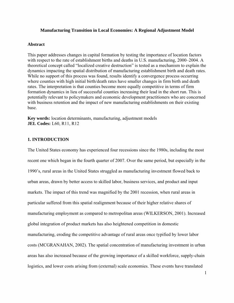
The frequency distribution of single-unit establishment birth and death rates across U.S.
counties in 2004 is shown in Figure 1. The frequencies are listed for all counties and by county
type: metropolitan, micropolitan, and non-core (U.S. CENSUS BUREAU, 2008). The z-axis,
labeled “Frequency”, has been truncated to 100 in order to better show the distribution of birth
and death rates at lower frequencies. Approximately 57% of all U.S. counties reported birth and
death rates lower than 10% of the manufacturing stock. The distribution for metropolitan and
micropolitan counties is similar. Non-core counties have more variation in birth and death rates,
8 The modifiable areal unit problem would also be a much more persistent issue of concern if counts of births and deaths were used in place of rates (OPENSHAW and TAYLOR, 1981).

14
which is likely due to their lower absolute levels of manufacturing activity. Figure 1 shows a
rather symmetric relationship between birth and death rates among all county types.
The location factors hypothesized to impact the spatial distribution of establishment birth
and death rates are reported in Table 2. Agglomeration economies are important factors in firms’
location decisions (COUGHLIN et al., 1991; WOODWARD, 1992; AUDRETSCH and
FRITSCH, 1999; ARMINGTON and ACS, 2002; DE GROOT et al., 2007). Agglomeration is
measured in the year 2000 with the percentage of manufacturing establishments with less than 10
employees, manufacturing’s share of employment in a county, percentage of manufacturing
establishments with more than 100 employees, and total business establishment density scaled by
county area. The first two measures are proxies for local agglomeration economies. The third and
fourth measures are intended to capture economies of scale internal to the firm and urbanization
economies, respectively. All four measures are hypothesized to have a positive impact on firm
location choice, and thus result in a higher incidence of birth in a county. Their effect on
establishment death is unknown a priori. Sector-specific employment data are from the U.S.
Department of Transportation commuting patterns compiled by the Research and Innovation
Technology Administration (RITA). Total firm density and percentage of manufacturing
establishments with less than 10 and more than 100 employees are calculated from the annual
County Business Patterns files.
Market structure is often the most important factor in investment location decisions
(BLAIR and PREMUS, 1987; CRONE, 1997). A county with more wealth and people increases
the likelihood of being a demand center for goods and services. Demand markets may also
harbor a relatively larger stock of creative individuals capable of solving difficult supply issues
or combining old ideas in a novel way, which may stimulate establishment birth (WOJAN and

15
MCGRANAHAN, 2007). Median household income, population, and the share of workers in
creative occupations are used to measure the market structure of a county (all measured in
2000).9
Labor is frequently cited as an important location factor impacting the spatial distribution
of firms (COUGHLIN and SEGEV, 2000; GUIMARÃES et al., 2004). Labor availability and
labor cost are measured by county unemployment rates (Bureau of Labor Statistics, BLS) and the
average wage per job (from the BEA), respectively. A high unemployment rate is hypothesized
to attract manufacturing investment, whereas a high average wage per job increases labor costs,
which deters investment. Additionally, the availability of skilled labor is measured by the
percentage of a county’s population 25 years of age and older with an associate degree. Labor
may also be sourced from neighboring counties. Net flows of wages per commuter between
place of residence and place of work help identify counties that are labor sources or sinks.
Access and breadth of infrastructure are measured by density of public roads and miles of
interstate highway with data from the U.S. Department of Transportation (DOT). Infrastructure
quality is measured by per capita local government expenditures on highways (CENSUS of
GOVERNMENTS, 1997). Available land is measured as the percentage of a county’s total area
in use as farmland, which is hypothesized to attract investment as the availability of land
increases. Presumably, farmland may be converted to other uses following sufficient investment
in infrastructure. This measure is calculated using a GIS database from ArcGIS 9.2 produced by
ESRI. For some counties, farmland area was not disclosed due to the small number of farms. In
9 Median household income and population are measured in thousands to avoid large differences in scaling between other covariates. The creative class share of employment was constructed by MCGRANAHAN and WOJAN (2007) and is available at http://www.ers.usda.gov/Data/CreativeClassCodes/.
those cases, the value was approximated by multiplying the number of farms by the average farm
size measured in acres in that county.
Fiscal policy may impact the cost of conducting business in a region, yet supporting a
favorable business climate, while generating sufficient revenue to provide the necessary public
goods is often difficult for local governments (GABE and BELL, 2004). Firms may consider
other locations if tax rates are perceived as too high. Taxes may deter manufacturing investment
(WHEAT, 1986; BARTIK, 1989), but local spending may be attractive (GOETZ, 1997).
Government expenditures on education and highways on a per capita basis measure the level of
public goods often provided by local governments.
<< Insert Table 2 >>
6. RESULTS
We model the regional adjustment in manufacturing establishment birth and death rates
between 2000 and 2004 using 3,078 counties of the lower 48 United States. Several specification
tests were performed to select the general models of given in equation (3a,b). Wald tests on the
significance of local spatial spillovers (WX) were statistically significant in the birth equation
( , df =19) and death equation (318W 0 ==Bγ1251W 0 ==Dγ
, df = 19), using the queen first-order
contiguity matrix as neighboring criteria. The eigenvalues of the weights matrix range between –
1 and +1, which determines the appropriate bounds on the parameter space for the spatial
autoregressive parameters. The average number of links in W is 5.8, with 0.19% of its elements
non-zero. Tests on spatial heterogeneity failed to reject that location factors were same in
importance across the county types. However, we maintained metropolitan and micropolitan
counties as additional explanatory variables, with non-core omitted as the reference category
assuming that only the constants are different between the three categories. Durbin-Wu-Hausman
16
17
(DWH) tests of Di,t and Bi,t, in equations (3a) and (3b) failed to reject exogeneity.10 However, the
DWH tests were rejected for spatially lagged birth and death, WDi,t and WBi,t. Given the mixed
results, we maintain the endogeneity of Di,t and Bi,t on the basis of the theoretical argument rather
than the empirical evidence. Using an a-spatial specification, first-stage F-tests as well as Sargan
statistics for over-identification reveal that the population dynamics used to instrument birth and
death rates appear to be appropriate (see bottom of Table 3). The LM-error tests for spatial
dependence in the IV residuals rejected the absence of spatial error processes in the birth (LM =
51.78, df =1) and death (LM = 89.27, df =1) equations. Additionally, Wald tests for the joint
significance of the auto-regressive processes were significant in the birth (Wρ = λ = 0 = 9.68, df =
2) and death (Wρ = λ = 0 = 7.54, df = 2) equations.11
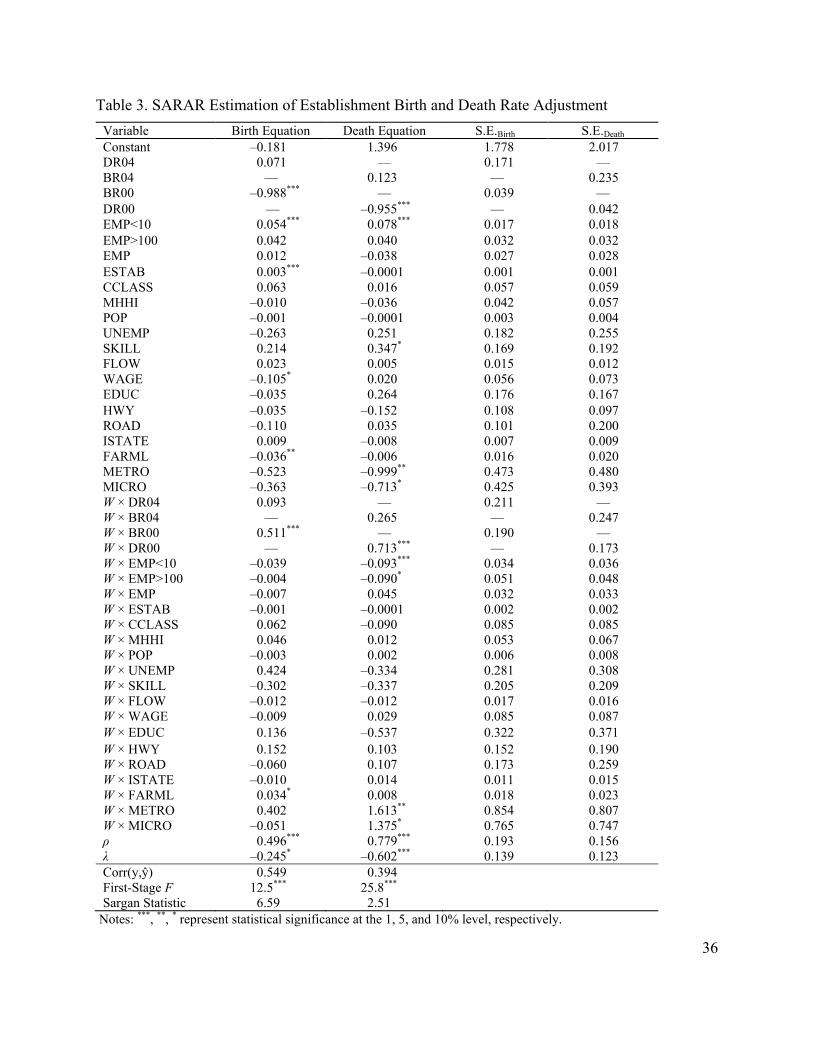
Results from the SARAR models are reported in Table 3. The SARAR model is
estimated using the R software, version 2.10.0.12 Standard errors, reported in the last two
columns, are robust against unspecified forms of heteroskedasticity. The second column of Table
2 shows the coefficients from the birth adjustment equation. Both spatial processes are
statistically significant. The coefficient on death rate (DR04) has the expected sign, but is not
statistically significant. This suggests that higher county establishment death rates did not lead to
significantly higher birth rates over the sample period. The coefficient on initial establishment
birth rate (BR00) suggests a convergence of birth rates from the initial period to the final period,
10 The endogeneity tests as well as tests for instrumental variable performance (first stage F-tests and Sargan statistics) were conducted on sets of equations estimated via OLS omitting spatially lagged dependent variables and spatially correlated errors. This is an obvious limitation, but endogeneity tests in the presence of spatial dependence are not presently available. 11 The Wald tests where implemented using the restrictions the ρ = λ = 0 in the birth and death equations from the SARAR model. 12 R is available for download at http://r-project.org (R Development Core Team, 2009). The R-code used to implement this estimator was originally developed by Vanessa Daniel of the Dept. of Spatial Economics at the VU University Amsterdam and members of the SHaPE group in the Dept. of Agricultural Economics at Purdue University.
18
but the coefficient on neighboring birth rates (W × BR00) suggests a momentum affect in the
adjustment process. Higher shares of manufacturing establishments with less than 10 employees
(EMP<10) and urban agglomeration (ESTAB) are correlated with increases in the establishment
birth rate between the two periods. However, higher wages per job (WAGE) and higher shares
of farmland (FARML) are negatively correlated with the birth rate adjustment process.
The death rate adjustment results are in the third column of Table 3. Both spatial
processes are also statistically significant in the death equation. The coefficient on birth rate
(BR04) has the expected sign, but is not significant. Firm birth rates do not appear to have a
direct impact on death rates. Taken together, there is no evidence of a creative destruction
process in manufacturing establishments over the current sample period. The coefficient on
initial establishment birth rate (DR00) also suggests a convergence of death rates from the initial
period to the final period, but the coefficient on neighboring death rates (W × DR00) also
suggests a momentum affect in the adjustment process. Higher shares of manufacturing
establishments with less than 10 employees (EMP<10) are correlated with increases in the
establishment death rate between the two periods. However, higher neighboring county shares
(W × EMP<10) are negatively correlated with death rate adjustments. Metropolitan (METRO)
and micropolitan (MICRO) counties have lower death rates compared to noncore counties.
However, neighboring metro (W × METRO) and micropolitan (W × MICRO) counties are
positively correlated with increases in establishment death rates compared to neighboring
noncore counties. Additional complexity in interpreting these results arises from the spatial
multiplier, (I – ρW), which moderates spatial decay between birth-death events between counties
(discussed in the next section).
<< Insert Table 3>>
6.1 Single-Unit Manufacturing Establishment Birth and Death Rates
Results from a spatial lag process model must be interpreted carefully. One standard
approach is to calculate the marginal effects of a change in an explanatory variable on the
dependent variable. LESAGE and PACE (2009) decompose the marginal effects into direct,
indirect, and total effects. The partial derivatives of the reduced form SARAR model in
equations (3a, b) are:
(4) 1( ) [y
I ].ρW W γk kxkβ−∂
= − + ⊗∂
where ⊗ is the element-wise (Hadamar) matrix product operator. The partial derivatives take the
form of an N by N matrix of marginal effects. The impact on the dependent variable from a
change in a covariate can be summarized in three ways (LESAGE and PACE, 2009). The first is
the average total effect on a spatial unit. The row sums are the total effect on each observation
from changing the k-th explanatory by one unit across all observations. Dividing the row sums
by the sample size yields the average total effect. The second impact is referred to as the direct
effect, which is the effect of changes in the i-th location of xk on yi including feedback effects on
the i-th through spillovers to other locations. The average direct effect is measured by summing
the trace of the N by N matrix in equation (4) and dividing by the sample size. The third impact
is referred to as the indirect effect, which constitutes spillover effects of neighbors.
<< Insert Table 4 >>
Marginal effects calculated from the SARAR model are reported in Table 4. The standard
errors of the direct, indirect, and total effects were estimated using a bootstrap procedure with
19

20
500 iterations.13 We focus most of the discussion on total effects. Coefficients of the direct,
indirect, and total effects of the initial period birth and death rates are negative and statistically
significant. This suggests a convergence process that takes place between the two time periods.
The interpretation is that counties with higher birth/death rates in a previous period will have
lower birth/death rates in the future period as convergence occurs. The percentage of
establishments with less than 10 employees (EMP<10) is positive and significant in the birth and
death rate adjustment equations, which suggests that a low barrier to entry leads to more
establishment births and is also a barrier to exit. Higher average wages (WAGE) have negative
effects on manufacturing establishment birth rates, but have positive effects on establishment
deaths. This illustrates the complexity that higher wages have on the dynamics of firm formation.
Similarly, interstate transportation infrastructure (ISTATE) has positive effects in adjustment of
birth rates and negative effects in adjustment of death rates. Such a result suggests that more
infrastructure may lead to a growth in the overall number of manufacturing establishments. Next,
we explore a policy experiment using the results of the SARAR model and the decomposition of
its marginal effects.
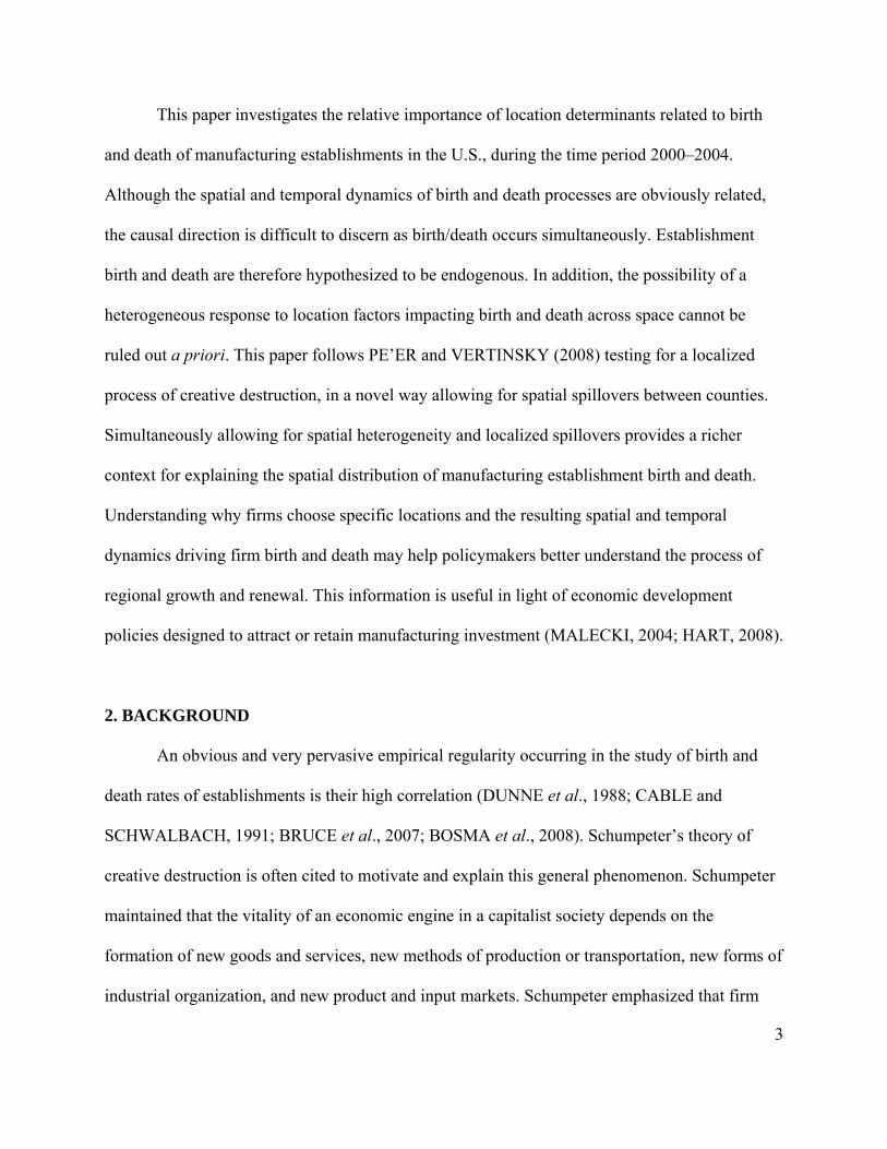
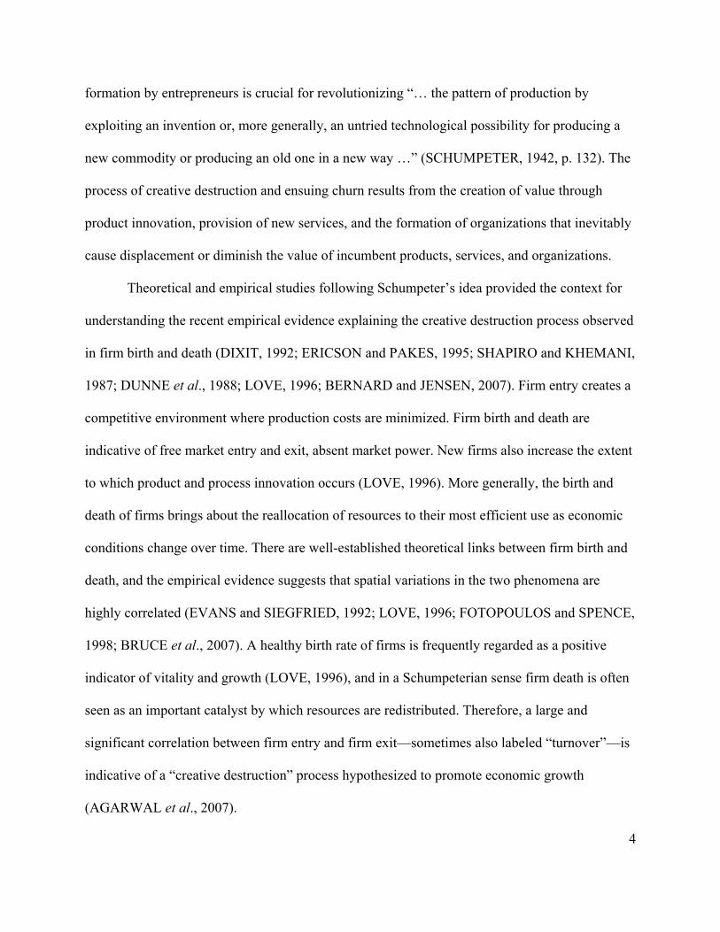
6.2 Metropolitan Spillovers Impacting Manufacturing Establishment Birth and Death Rates
Policymakers and regional economic development practitioners may be interested in
knowing how changes in metropolitan counties spillover to non-metropolitan counties. Spatial
process models are capable of analyzing such situations. Spatial cluster analysis was conducted
using Local Indicators of Spatial Association (LISA, Anselin, 1995) to determine if the pattern of
13 The data generating process of the SARAR model was used to sample with replacement from the residuals of the IV model in order to reconstruct the dependent variable and re-estimate the SARAR model 500 times. Results of the bootstrapping were stored in matrices in order to calculate average direct, indirect, and total effects over the iterations.
21
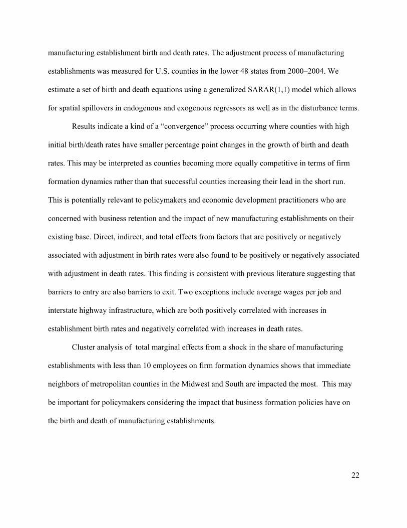
spillovers between interconnected metro and non-metro counties demonstrated a greater
likelihood of adjustment in firm dynamics relative to other counties.14 We select the share of
manufacturing establishments with less than 10 employees (EMP<10) to shock because it is a
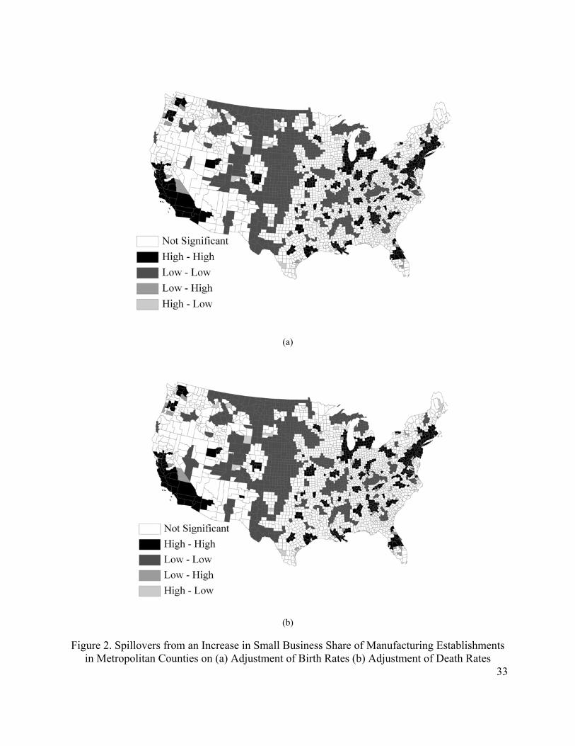
significant covariate in both the birth and death equations. Figure 2 shows how a 2% increase in
the total effects of EMP<10 in metro counties spills over into non-metro counties, impacting the
adjustment of (a) manufacturing establishment birth rates and (b) establishment death rates.
Given that the coefficient on EMP<10 is similar in magnitude and sign in the birth and death
equations, we expect to see a similar pattern in the spillovers from metro to non-metro counties.
Figure 2a and 2b both show that significant spillovers attenuate to the immediate neighbors of
metropolitan counties and quickly become insignificant thereafter. Non-metro counties in the
Midwest and the South appear to capture the most from increases in small manufacturing
establishment spillovers emanating from metropolitan counties as shown by the low-high LISA
category of the map. This result may be due to the predominance of the manufacturing sector in
those regions, but may be important for policymakers considering the impact that business
formation policies have on the birth and death of manufacturing establishments.
<< Insert Figure 2 >>
7. CONCLUSIONS
This paper contributes to the empirical literature examining manufacturing establishment
birth and death using a regional adjustment model and spatial econometrics. Localized creative
destruction was tested as a mechanism to explain the adjustment of the spatial distribution of
14 Lambert et al. (2006b) use a similar method for comparing food manufacturing clusters, but the clusters were based on location probabilities estimated by probit regression.
22
manufacturing establishment birth and death rates. The adjustment process of manufacturing
establishments was measured for U.S. counties in the lower 48 states from 2000–2004. We
estimate a set of birth and death equations using a generalized SARAR(1,1) model which allows
for spatial spillovers in endogenous and exogenous regressors as well as in the disturbance terms.
Results indicate a kind of a “convergence” process occurring where counties with high
initial birth/death rates have smaller percentage point changes in the growth of birth and death
rates. This may be interpreted as counties becoming more equally competitive in terms of firm
formation dynamics rather than that successful counties increasing their lead in the short run.
This is potentially relevant to policymakers and economic development practitioners who are
concerned with business retention and the impact of new manufacturing establishments on their
existing base. Direct, indirect, and total effects from factors that are positively or negatively
associated with adjustment in birth rates were also found to be positively or negatively associated
with adjustment in death rates. This finding is consistent with previous literature suggesting that
barriers to entry are also barriers to exit. Two exceptions include average wages per job and
interstate highway infrastructure, which are both positively correlated with increases in
establishment birth rates and negatively correlated with increases in death rates.
Cluster analysis of total marginal effects from a shock in the share of manufacturing
establishments with less than 10 employees on firm formation dynamics shows that immediate
neighbors of metropolitan counties in the Midwest and South are impacted the most. This may
be important for policymakers considering the impact that business formation policies have on
the birth and death of manufacturing establishments.
23
REFERENCES
ACS, Z.J. and ARMINGTON, C. (2004) Employment growth and entrepreneurial activity in
cities, Regional Studies 38, 911-927.
ACS, Z.J. and MUELLER, P. (2008) Employment effects of business dynamics: mice, gazelles,
and elephants, Small Business Economics 30, 85-100.
AGARWAL, R., AUDRETSCH, D. and SARKAR, M.B. (2007) The process of creative
destruction : knowledge spillovers, entrepreneurship, and economic growth, Strategic
Entrepreneurship Journal 1, 263-286.
ANSELIN, L. (1988) Spatial Econometrics: Methods and Models. London, Kluwer Academic
Publishers.
ANSELIN, L. (1995) Local indicators of spatial association - LISA, Geographical Analysis 27,
93-115.
ANSELIN, L. (2002) Under the hood: issues in the specification and interpretation of spatial
regression models, Agricultural Economics 17 (3), 247-267.
ANSELIN, L. and KELEJIAN, H.H. (1997) Testing for spatial error autocorrelation in the
presence of endogenous regressors, International Regional Science Review 20(1&2),
153-182.
ARMINGTON, C. and ACS, Z.J. (2002) The determinants of regional variation in new firm
formation, Regional Studies 36(1), 33-45.
ARRAIZ, I., DRUKKER, D.M., KELEJIAN, H.H., and PRUCHA, I.R. (2008) A spatial Cliff-
Ord type model with heteroskedastic innovations: small and large sample results,
CESIFO Working Paper no. 2485.

24
AUDRETSCH, D.B. (1990) Start-up size and establishment exit, Discussion Paper FS IV 90-8,
Wissenschaftszentrum Berlin.
AUDRETSCH, D.B. and FRITSCH, M. (1992) Market dynamics and regional development in
the Federal Republic of Germany, Discussion Paper FS IV 92-6,Wissenschaftszentrum
Berlin.
AUDRETSCH, D.B. and FRITSCH, M. (1994) On the measurement of entry rates, Empirica 21,
105-113.
AUDRETSCH, D.B. and FRITSCH, M. (1999) The industry component of regional new firm
formation processes, Review of Industrial Organization 15, 239-252.
AUSTIN, J.S. and ROSENBAUM, D.I. (1990) The determinants of entry and exit rates into
U.S. manufacturing industries, Review of Industrial Organization 5(2), 211-23.
BALDWIN, J.R. and GORECKI, P.K. (1991) Firm entry and exit in the Canadian
manufacturing sector, The Canadian Journal of Economics 24(2), 300-323.
BARTIK, T.J. (1989) Small business start–ups in the United States: estimates of the effects of
characteristics of states, Southern Economic Journal 55(4), 1004-1018.
BARTELSMAN, E., SCARPETTA, S. and SCHIVARDI, F. (2003) Comparative analysis of
firm demographics and survival: micro-level evidence for the OECD countries,
OCED Economics Department, WP No. 348.
BAUM, J.A.C. (1996) Organizational ecology, in: CLEGG, S., HARDY, C., NORD, W. (Eds)
Handbook of Organization Studies. Sage, London.
BERNARD, A.B. and JENSEN, J.B. (2007) Firm structure, multinationals, and manufacturing
plant deaths, The Review of Economics and Statistics 89(2), 193-204.

25
BLAIR, J.P., PREMUS, R. (1987) Major factors in industrial location: a review, Economic
Development Quarterly 1(1), 72–85.
BOARNET, M.G. (1994a) An empirical model of intermetropolitan population and
employment growth, Papers in Regional Science 73, 135-52.
BOARNET, M.G. (1994b) The Monocentric model and employment location, Journal of Urban
Economics 36, 79-97.
BOSMA, N., STAM, E. and SCHUTJENS, V. (2008) Creative destruction and regional
productivity growth: evidence from the Dutch manufacturing and services industries.
Papers in Evolutionary Economic Geography # 08.13, Utrecht University, Urban and
Regional Research Center.
BRUCE, D., DESKINS, J.A. HILL, B.C. and RORK, J.C. (2007) Small business and state
growth: an econometric investigation, Small Business Administration: Office of
Advocacy. Report No. 292.
CABLE, J. and SCHWALBACH, J. (1991) International comparisons of entry and exit, in:
GEROSKI, P. and SCHWALBACH, J. (Eds) Entry and Market Contestability: An
International Comparison. Blackwell, Oxford.
CARLINO, G.A. and MILLS, E.S. (1987) The determinants of county growth, Journal of
Regional Science 27, 39-54.
CARRUTHERS, J.I. and MULLIGAN, G.F. (2007) Land absorption in U.S. metropolitan
areas: estimates and projections from regional adjustment models, Geographical
Analysis 39, 78-104.
CARRUTHERS, J.I. and VIAS, A.C. (2005) Urban, suburban, and exurban sprawl in the
Rocky Mountain West, Journal of Regional Science 45, 21-48.
26
CLARK, D.E. and MURPHY, C.A. (1996) Countywide employment and population growth:
an analysis of the 1980s, Journal of Regional Science 36, 235-56.
COUGHLIN, C.C. and SEGEV, E. (2000) Location determinants of new foreign owned
manufacturing plants, Journal of Regional Science 40, 323-351.
COUGHLIN, C.C., TERZA, J.V. and ARROMDEE, V. (1991) State characteristics and the
location of foreign direct investment within the United States, The Review of
Economics and Statistics 73, 675-683.
CRONE, T.M. (1997) Where have all the factory jobs gone - and why?, Business Review,
Federal Reserve Bank of Philadelphia, May/June.
DE GRAAFF, T., FLORAX, R.J.G.M., NIJKAMP, P. and REGGIANI, A. (2001) A general
misspecification test for spatial regression models: dependence, heterogeneity, and
nonlinearity, Journal of Regional Science 41(2), 255-76.
DE GROOT, H.L.F., POOT, J. and SMIT, M.J. (2007) Agglomeration, innovation, and regional
development: theoretical perspectives and meta-analysis, Tinbergen Institute
Discussion Paper 079/3.
DIXIT, A. (1992) Investment and hysteresis, The Journal of Economic Perspectives 6(1), 107-
32.
DUNNE, T., ROBERTS, M.J. and SAMUELSON, L. (1988) Patterns of firm entry and exit in
U.S. manufacturing industries, RAND Journal of Economics 19(4), 495-515.
DURBIN, J. (1954) Errors in variables, Review of the International Statistical Institute. 22, 23-
32.
ERICSON, R. and PAKES, A. (1995) Markov-perfect industry dynamics: a framework for
empirical work, Review of Economic Studies 62, 53-82.
27
EVANS, L.B. and SIEGFRIED, J.J. (1992) Entry and exit in United States manufacturing
industries from 1977 to 1982, in AUDRETSCH, D.B. and SIEGFRIED, J.J. (Eds)
Empirical Studies in Industrial Organization: Essays in Honour of Leonard W. Weiss, pp.
253-73. Kluwer, Netherlands.
FIGUEIREDO, O., GUIMARÃES, P., and WOODWARD, D. (2002) Home–field advantage:
location decisions of Portuguese entrepreneurs, Journal of Urban Economics 52, 341–
61.
FLORAX, R.J.G.M., and FOLMER, H. (1992) Specification and estimation of spatial linear
regression models: monte carlo evaluation of pre-test estimators, Regional Science
and Urban Economics 22, 405-32.
FOTOPOULOS, G. and SPENCE, N. (1998) Entry and exit from manufacturing industries:
symmetry, turbulence and simultaneity – some empirical evidence from Greek
manufacturing industries, 1982 – 1988, Applied Economics 30, 245-62.
FRITSCH, M. (1997). New firms and regional employment change, Small Business Economics
9, 437-448.
GABE, T., and BELL , K.P. (2004) Tradeoffs between local taxes and government spending as
determinants of business location, Journal of Regional Science 44(1), 21–41.
GEROSKI, P.A. (1995) What do we know about entry?, International Journal of Industrial
Organization 13, 421-440.
GOETZ, S. (1997) State- and county-level determinants of food manufacturing establishment
growth: 1987-1993, American Journal of Agricultural Economics 79(3), 838-50.
GUIMARÃES, P., FIGUEIREDO, O., WOODWARD, D. (2004) Industrial location modeling:
extending the random utility framework, Journal of Regional Science 44(1), 1–20.
28
HALL, B.H. (1987) The relationship between firm size and firm growth in the US
manufacturing sector, Journal of Industrial Economics 35, 583-605.
HAMERMESH D. S. (1993) Labor Demand. New Jersey: Princeton University Press.
HART, D.M. (2008) The politics of ‘entrepreneurial’ economic development policy of states
in the U.S., Review of Policy Research 25(2), 149–68.
HAUSMAN, J.A. (1978) Specification tests in econometrics, Econometrica 46, 931-959.
HENDERSON, J.R. and MCNAMARA, K.T. (1997) Community attributes influencing local
food processing growth in the U.S.Corn Belt, Canadian Journal of Agricultural
Economics 45, 235-50.
HOOGSTRA, G.J., VAN DIJK and FLORAX, R.J.G.M. (2010) Determinants of variation in
population-employment interaction findings: a quasi-experimental meta-analysis.
Geographical Analysis. In press.
HOPENHAYM, H.A. (1992) Entry, exit, and firm dynamics in long run equilibrium,
Econometrica 60(5), 1127-1150.
JOHNSON, P. and PARKER, S. (1996) Spatial variations in the determinants and effects of
firm births and deaths, Regional Studies 30(7), 679-688.
JOVANOVIC, B. (1982) Selection and the evolution of industry, Econometrica 50, 649-70.
KANGASHARJU, A. and MOISIO, A. (1998) Births-deaths nexus of firms: estimating VAR
with panel data, Small Business Economics 11, 303-313.
KELEJIAN, H.H. and PRUCHA, I.R. (2007) Specification and estimation of spatial
autoregressive models with autoregressive and heteroskedastic disturbances, forthcoming
in Journal of Econometrics.
29
LAMBERT, D.M., GARRET, M.I., MCNAMARA, K.T. (2006a) An application of spatial
Poisson models to manufacturing investment location analysis, Journal of Agricultural
and Applied Economics 38(1), 105–121.
LAMBERT, D.M., GARRET, M.I., MCNAMARA, K.T. (2006b) Food industry investment
flows: implications for rural development, Review of Regional Studies 36(2), 140-162.
LAZEAR, EDWARD P. (2002) Entrepreneurship, National Bureau of Economic Research
Working Paper 9109, August.
LOVE, J.H. (1996) Entry and exit: a county-level analysis, Applied Economics 28, 441-451.
MALECKI, E.J. (2004) Jockeying for position: what it means and why it matters to regional
development policy when places compete, Regional Studies 38, 1101–20.
MCGRANAHAN, D.A. (2002) Local context and advanced technology use by small,
independent manufacturers in rural areas, American Journal of Agricultural Economics
84(5), 1237-1245.
OPPENSHAW S., TAYLOR P.J. (1981) The modifiable areal unit problem. In: WRIGLEY N.,
BENNETT R.J., (Eds) Quantitative Geography. London, United Kingdom: Routledge
and Kegan Paul.
PAKES, A. and ERICSON, R. (1998) Empirical iImplications of alternative models of firm
dynamics, Journal of Economic Theory 79, 1-45.
PE’ER, A. and VERTINKSY, I. (2008) Firm exits as a determinant of new entry: is there
evidence of local creative destruction?, Journal of Business Venturing 23, 280-306.
PHILIPS, B.D. and KIRKOFF, B.A. (1989) Formation, growth, and survival: small
firm dynamics in the U.S. economy, Small Business Economics 1, 65-74.

30
REYNOLDS, P.D., MILLER, B. and MAKI, W.R. (1995) Explaining regional variation in
business births and deaths: U.S. 1976-88, Small Business Economics 7, 389-407.
SCHUMPETER, J.A. (1942) Socialism and Democracy. New York: Harper.
SHAPIRO, D. and KHEMANI, R.S. (1987) The determinants of entry and exit reconsidered,
International Journal of Industrial Organization 5, 15-26.
STEINNES, D.N. and FISHER,W.D. (1974) An econometric model of interurban location,
Journal of Regional Science 14, 65-80.
STINCHCOMBE, A.L. (1965) Social structures and organizations. In: March, J.G. (Ed.)
Handbook of Organizations, Rand McNally, Chicago.
STOREY, D.J. and JONES, A.M. (1987) New firm formation – A labour market approach to
industrial entry, Scottish Journal of Political Economy 34, 37-51.
U.S. CENSUS BUREAU (2008) Metropolitan and micropolitan statistical areas, Available at:
http://www.census.gov/population/www/metroareas/metrodef.html.
U.S. CENSUS BUREAU, Company Statistics Division (2008) Statistics of U.S. businesses:
dynamic data. Available at: http://www.census.gov/csd/susb/susbdyn.htm. Accessed on
5/23/2008.
U.S. CENSUS BUREAU (1997) Census of Governments, Available at:
http://www.census.gov/govs/www/cog97.html. Accessed on 10/21/2008.
U.S. CENSUS BUREAU (2003) Metropolitan and Micropolitan Statistical Areas. Available at:
http://www.census.gov/population/www/metroareas/metrodef.html.
U.S. DEPARTMENT OF TRANSPORTATION (2000), Federal highway administration.
highway statistics 2000. Available at: http://www.fhwa.dot.gov/ohim/hs00/re.htm.
Accessed on 3/11/2008.
31
WHEAT, L. (1986) The determinants of 1963–77 regional manufacturing growth: why the South
and West grow, Journal of Regional Science 26(4), 635 – 660.
WILKERSON, C. (2001) Trends in rural manufacturing. The Main Street Economist, Center for
the Study of Rural America. Federal Reserve Bank of Kansas City.
WOJAN, T.R., MCGRANAHAN, D.A. (2007) Ambient returns: creative capital's contribution
to local manufacturing competitiveness, Agricultural and Resource Economics Review
36(1), 133-148.
WOODWARD, D.P. (1992) Location determinants of Japanese manufacturing start–ups in the
United States, Southern Economics Journal 58, 690 –708.
WU, D. (1973) Alternative tests of independence between stochastic regressors and
disturbances, Econometrica 41-4, 733-749.

All Counties Metropolitan Counties
Micropolitan Counties Non-core Counties
Figure 1. Frequency of Single-Unit Establishment Birth and Death Rates in U.S. Counties, in
2004
32
(a)
(b)
33
Figure 2. Spillovers from an Increase in Small Business Share of Manufacturing Establishments in Metropolitan Counties on (a) Adjustment of Birth Rates (b) Adjustment of Death Rates

Table 1. Model specification and hypotheses Hypothesis Restrictions Degrees of
Freedom Test Statistic
Creative destruction α1 = 0 δ1 = 0
1 1
Wald Wald
Local creative destruction γ1 = 0 τ1 = 0
1 1
Wald Wald
Local spatial spillovers γ1 = γ2 = γB = 0 τ1 = τ2 = τD = 0
19 19
Wald Wald
Slope homogeneity of metropolitan, micropolitan, and noncore counties
Birth: β – βr = 0 Death: β – βr = 0
74 74
Wald Wald
Spatial lag process ρ1 = 0 ρ2 = 0
1 1
Wald Wald
Spatial error process λ1 = 0 λ2 = 0
1 1
Wald Wald
Spatial lag and error processes ρ1 = λ1 = 0 ρ2 = λ2 = 0
2 2
Wald Wald
Error correlation between birth-death equations
Corr( ) = 0 DBii εε , [n ×(n-1)] / 2 LM
34

Table 2. Descriptive Statistics Birth and Death Rate Model Variables Label Average Stdev
Manuf. share of employment (%) EMP 15.19 10.35 Manuf. establishments with less than 10 emp.(%) EMP<10 52.11 19.99 Manuf. establishments with more than 100 emp. (%) EMP>100 11.05 9.93 Total establishment density (estab. per square mile) ESTAB 5.21 59.98 Creative class share of employment CCLASS 17.18 5.94 Median household income (1,000 $) MHHI 32.01 87.41 Population (1,000) POP 91.04 295.68 Average wage per job (1,000 $) WAGE 24.69 5.59 Unemployment Rate (%) UNEMP 4.32 1.64 Associate's Degree (% of population 25 years +) SKILL 5.70 1.99 Public road density ROAD 1.84 1.52 Interstate (miles) ISTATE 14.68 25.23 Available land (% farm area/total area) FARML 31.29 25.96 Highway per capita expenditures (100 $) HWY 1.77 2.50 Education spending per capita (1,000 $) EDUC 1.18 1.17 Metropolitan county METRO 0.34 0.48 Micropolitan county MICRO 0.22 0.41 Noncore county NONCORE 0.44 0.50 Single-unit birth rate in 2000 (%) BR00 6.44 8.75 Single-unit death rate in 2000 (%) DR00 6.68 7.66 Single-unit birth rate in 2004 (%) BR04 5.90 7.72 Single-unit death rate in 2004 (%) DR04 6.45 8.21 N = 3,078
35
36
Table 3. SARAR Estimation of Establishment Birth and Death Rate Adjustment Variable Birth Equation Death Equation S.E.Birth S.E.Death
Constant –0.181 1.396 1.778 2.017 DR04 0.071 — 0.171 — BR04 — 0.123 — 0.235 BR00 –0.988*** — 0.039 — DR00 — –0.955*** — 0.042 EMP<10 0.054*** 0.078*** 0.017 0.018 EMP>100 0.042 0.040 0.032 0.032 EMP 0.012 –0.038 0.027 0.028 ESTAB 0.003*** –0.0001 0.001 0.001 CCLASS 0.063 0.016 0.057 0.059 MHHI –0.010 –0.036 0.042 0.057 POP –0.001 –0.0001 0.003 0.004 UNEMP –0.263 0.251 0.182 0.255 SKILL 0.214 0.347* 0.169 0.192 FLOW 0.023 0.005 0.015 0.012 WAGE –0.105* 0.020 0.056 0.073 EDUC –0.035 0.264 0.176 0.167 HWY –0.035 –0.152 0.108 0.097 ROAD –0.110 0.035 0.101 0.200 ISTATE 0.009 –0.008 0.007 0.009 FARML –0.036** –0.006 0.016 0.020 METRO –0.523 –0.999** 0.473 0.480 MICRO –0.363 –0.713* 0.425 0.393 W × DR04 0.093 — 0.211 — W × BR04 — 0.265 — 0.247 W × BR00 0.511*** — 0.190 — W × DR00 — 0.713*** — 0.173 W × EMP<10 –0.039 –0.093*** 0.034 0.036 W × EMP>100 –0.004 –0.090* 0.051 0.048 W × EMP –0.007 0.045 0.032 0.033 W × ESTAB –0.001 –0.0001 0.002 0.002 W × CCLASS 0.062 –0.090 0.085 0.085 W × MHHI 0.046 0.012 0.053 0.067 W × POP –0.003 0.002 0.006 0.008 W × UNEMP 0.424 –0.334 0.281 0.308 W × SKILL –0.302 –0.337 0.205 0.209 W × FLOW –0.012 –0.012 0.017 0.016 W × WAGE –0.009 0.029 0.085 0.087 W × EDUC 0.136 –0.537 0.322 0.371 W × HWY 0.152 0.103 0.152 0.190 W × ROAD –0.060 0.107 0.173 0.259 W × ISTATE –0.010 0.014 0.011 0.015 W × FARML 0.034* 0.008 0.018 0.023 W × METRO 0.402 1.613** 0.854 0.807 W × MICRO –0.051 1.375* 0.765 0.747 ρ 0.496*** 0.779*** 0.193 0.156 λ –0.245* –0.602*** 0.139 0.123 Corr(y,ŷ) 0.549 0.394 First-Stage F 12.5*** 25.8*** Sargan Statistic 6.59 2.51
Notes: ***, **, * represent statistical significance at the 1, 5, and 10% level, respectively.

37
Table 4. Marginal Effects from SARAR Model Birth Equation Death Equation Variable Direct Indirect Total Effect Direct Indirect Total Effect
DR04 0.007 0.743 0.750 ─ ─ ─ BR04 ─ ─ ─ 0.109*** 1.012*** 1.121***
BR00 –1.276*** –6.039 –7.315* ─ ─ ─ DR00 ─ ─ ─ –1.328*** –3.699*** –5.027*** EMP<10 0.076*** 0.331 0.406* 0.113*** 0.286*** 0.399***
EMP>100 0.057*** 0.421 0.478* 0.057*** 0.353*** 0.410***
EMP 0.009** –0.209 –0.200 –0.050*** –0.138*** –0.188*** ESTAB 0.004*** 0.026 0.030* 0.0001 0.0001 0.0002 CCLASS 0.071*** 0.279 0.350 0.037*** 0.237*** 0.274***
MHHI –0.018*** 0.117 0.099 –0.075*** –0.221*** –0.296*** POP –0.001 0.023 0.022 0.0002 0.003 0.004 UNEMP –0.369*** –1.025 –1.394 0.411*** 1.023*** 1.434***
SKILL 0.324*** 1.367 1.691 0.552*** 1.392*** 1.944***
FLOW 0.030*** 0.224 0.254 0.013*** 0.034*** 0.047***
WAGE –0.126*** –0.454* –0.580** 0.033*** 0.077* 0.110**
EDUC –0.054*** 0.711 0.657 0.406*** 1.012*** 1.418***
HWY –0.073*** –0.904 –0.976* –0.259*** –0.666*** –0.925*** ROAD –0.153*** –0.759* –0.912 0.038*** 0.079 0.117 ISTATE 0.012*** 0.070 0.083** –0.011*** –0.070*** –0.080*** FARML –0.050*** –0.165 –0.215 –0.011*** –0.025*** –0.036*** METRO –0. 643*** 0.081 –0.562 –1.651*** –4.106*** –5.757*** MICRO –0.440*** –1.458 –1.898* –0.840*** –2.013*** –2.853*** Notes: ***, **, * represent statistical significance at the 1, 5, and 10% level, respectively. Standard errors are not reported to conserve space.