many-electron effects in the extended x-ray absorption fine structure
TRANSCRIPT

Many-Electron Effects in the Extended X-ray Absorption
Fine Structure
A thesis submitted for the degree of
Doctor of Philosophy
at the University of Leicester
by
Mervyn Roy
Department of Physics and Astronomy
University of Leicester
August 1999

Many-Electron Effects in the Extended X-ray Absorption
Fine Structure
by
Mervyn Roy
Abstract
Extended X-ray absorption fine structure (EXAFS) spectroscopy is an experimentaltechnique useful in the study of non-crystalline materials. EXAFS is analysed bycomparing experimental to theoretical spectra. Many-electron effects in EXAFSare important, however, EXAFS theory has been developed using a single electronformalism with many-body effects included via empirical factors. Multiple electronexcitations reduce the EXAFS amplitude and hence affect the determination ofcoordination numbers. At present, intrinsic amplitude reduction effects are modelledby a constant factor whilst extrinsic effects are modelled using an imaginary scatteringpotential or mean free path term.
This thesis is concerned with the many electron effects in EXAFS. Expressions aredeveloped with which the EXAFS amplitude may be studied independently in thepresence of a complex scattering potential. The Hedin-Lundqvist [9] potential, whichis most commonly used in EXAFS analysis, is found to overestimate the extrinsiclosses but fortuitously gives good agreement to the total losses to the EXAFS. It isconcluded that an intrinsic reduction factor should not be used when data fitting withthis potential. The Beni, Lee and Platzman [18] correlation potential is also investigatedand found to be unsuitable for EXAFS calculations.
The intrinsic amplitude reduction factor is calculated in the high energy limit forall elements and found to give good agreement with experiment. Calculations withboth tight binding and atomic initial state wavefunctions show that chemical effectsare unimportant when determining the intrinsic amplitude reduction factor.
Time-dependent perturbation theory and a model form for the core hole -photoelectron system are used to calculate the multiple electron excitations followinga photoabsorption. Screened and unscreened forms of the potential are investigated.The results agree well with experiment and may be used to approximate the amplitudelosses to the EXAFS without the need for ad hoc parameters or complex scatteringpotentials.

Contents
Acknowledgements vi
1 Introduction 1
1.1 The X-ray Absorption Coefficient . . . . . . . . . . . . . . . . . . 3
1.2 The EXAFS . . . . . . . . . . . . . . . . . . . . . . . . . . . . . . 6
1.3 Many-Body Effects . . . . . . . . . . . . . . . . . . . . . . . . . . 8
1.3.1 Inelastic Effects . . . . . . . . . . . . . . . . . . . . . . . . 10
1.4 Synopsis of the Thesis . . . . . . . . . . . . . . . . . . . . . . . . 13
2 The X-ray Absorption Fine Structure 17
2.1 Background . . . . . . . . . . . . . . . . . . . . . . . . . . . . . . 20
2.1.1 The Muffin Tin Potential . . . . . . . . . . . . . . . . . . . 20
2.1.2 The Green Function . . . . . . . . . . . . . . . . . . . . . 20
2.1.3 The Regular Solution . . . . . . . . . . . . . . . . . . . . . 21
2.1.4 The Irregular Solution . . . . . . . . . . . . . . . . . . . . 23
2.1.5 The Initial States . . . . . . . . . . . . . . . . . . . . . . . 24
2.2 The Isolated Atom . . . . . . . . . . . . . . . . . . . . . . . . . . 25
2.2.1 A Real Scattering Potential . . . . . . . . . . . . . . . . . 25
2.2.2 A Complex Scattering Potential . . . . . . . . . . . . . . . 28
2.3 The EXAFS . . . . . . . . . . . . . . . . . . . . . . . . . . . . . . 32
ii

Contents iii
2.3.1 A Real Scattering Potential . . . . . . . . . . . . . . . . . 32
2.3.2 A Complex Scattering Potential . . . . . . . . . . . . . . . 36
2.4 Conclusion . . . . . . . . . . . . . . . . . . . . . . . . . . . . . . . 38
3 The Self-Energy and the Dielectric Function 39
3.1 Many-Body Physics . . . . . . . . . . . . . . . . . . . . . . . . . . 39
3.2 Screening . . . . . . . . . . . . . . . . . . . . . . . . . . . . . . . 41
3.3 The Self-Energy . . . . . . . . . . . . . . . . . . . . . . . . . . . . 43
3.4 The Inverse Dielectric Function . . . . . . . . . . . . . . . . . . . 47
3.4.1 The Local Inverse Dielectric Function . . . . . . . . . . . . 49
3.4.2 Free Electron Gas Calculation of ǫ−1(q, ω) . . . . . . . . . 50
3.4.3 LDA of an Average Single Plasmon Pole ǫ−1(q, ω). . . . . . 53
3.4.4 Atomic Calculation of ǫ−1(q, ω) . . . . . . . . . . . . . . . 54
3.4.5 The X-ray Absorption Coefficient . . . . . . . . . . . . . . 57
3.5 Results . . . . . . . . . . . . . . . . . . . . . . . . . . . . . . . . . 58
3.5.1 The Small q Limit . . . . . . . . . . . . . . . . . . . . . . 59
3.5.2 q Dependence . . . . . . . . . . . . . . . . . . . . . . . . . 62
3.6 Conclusion . . . . . . . . . . . . . . . . . . . . . . . . . . . . . . . 65
4 An Investigation of the Hedin-Lundqvist Exchange and
Correlation Potential 67
4.1 Calculation of the Potential . . . . . . . . . . . . . . . . . . . . . 68
4.1.1 The Self-Energy . . . . . . . . . . . . . . . . . . . . . . . . 68
4.1.2 The Exchange and Correlation Potential within the LDA . 70
4.2 Results . . . . . . . . . . . . . . . . . . . . . . . . . . . . . . . . . 74
4.2.1 The HL Potential . . . . . . . . . . . . . . . . . . . . . . . 74
4.2.2 The Average Potential . . . . . . . . . . . . . . . . . . . . 77
4.2.3 The Isolated Atom . . . . . . . . . . . . . . . . . . . . . . 79

Contents iv
4.2.4 EXAFS Amplitudes . . . . . . . . . . . . . . . . . . . . . . 81
4.3 Conclusion . . . . . . . . . . . . . . . . . . . . . . . . . . . . . . . 89
5 An Investigation of the Beni, Lee and Platzman Polarisation
Potential 90
5.1 Calculation of the Polarisation Potential . . . . . . . . . . . . . . 93
5.2 The Average Self-Energy . . . . . . . . . . . . . . . . . . . . . . . 96
5.3 Results . . . . . . . . . . . . . . . . . . . . . . . . . . . . . . . . . 99
5.3.1 The Imaginary Part . . . . . . . . . . . . . . . . . . . . . . 99
5.3.2 The Real Part . . . . . . . . . . . . . . . . . . . . . . . . . 106
5.3.3 A Self-Consistent Calculation . . . . . . . . . . . . . . . . 109
5.4 Conclusion . . . . . . . . . . . . . . . . . . . . . . . . . . . . . . . 111
6 The Core hole - Photoelectron System in the Sudden
Approximation 114
6.1 The Amplitude Reduction Factor . . . . . . . . . . . . . . . . . . 116
6.2 The EXAFS Function . . . . . . . . . . . . . . . . . . . . . . . . 117
6.3 Results . . . . . . . . . . . . . . . . . . . . . . . . . . . . . . . . . 120
6.3.1 Free Atom Calculation of s2o . . . . . . . . . . . . . . . . . 120
6.3.2 Shake Probabilities . . . . . . . . . . . . . . . . . . . . . . 124
6.4 The Chemical Dependence of s2o . . . . . . . . . . . . . . . . . . . 126
6.4.1 Tight Binding Method . . . . . . . . . . . . . . . . . . . . 126
6.5 Conclusion . . . . . . . . . . . . . . . . . . . . . . . . . . . . . . . 133
7 A Time-Dependent Model of the Core hole - Photoelectron
System 134
7.1 Theory . . . . . . . . . . . . . . . . . . . . . . . . . . . . . . . . . 136
7.1.1 Shake-off Intensities and the Sudden Approximation . . . . 139

Contents v
7.1.2 A Screened Core Hole Potential . . . . . . . . . . . . . . . 144
7.1.3 The Two Electron Absorption Coefficient . . . . . . . . . . 149
7.2 Results . . . . . . . . . . . . . . . . . . . . . . . . . . . . . . . . . 152
7.2.1 Calculation of γ . . . . . . . . . . . . . . . . . . . . . . . . 153
7.2.2 Secondary Electron Shake-off Probabilities . . . . . . . . . 154
7.2.3 The Ejected Electron Spectrum . . . . . . . . . . . . . . . 164
7.2.4 The Two Electron Photoionisation Cross Section . . . . . 166
7.2.5 The Two Electron Absorption Coefficient . . . . . . . . . . 168
7.2.6 The Amplitude Reduction Factor . . . . . . . . . . . . . . 169
7.2.7 Connection with EXAFS Data Analysis . . . . . . . . . . . 173
7.3 Conclusion . . . . . . . . . . . . . . . . . . . . . . . . . . . . . . . 176
8 Summary and Conclusions 178
A The Real Part Of The Hedin-Lundqvist Potential 183
B Derivation of the Beni, Lee and Platzman Polarisation Potential
from the Atomic Scattering Factor 185
C Calculation of an using a Different q Dependent Plasmon
Frequency. 189
Acknowledgements
I would like to express my thanks to the members of the Theory group at
Leicester for making my time here so enjoyable. In particular to Prof. John
Beeby, Dr Peter Maksym, Dr Neil Bruce, Sean Pearson, Frank Hart and Gary
Mallon.
I would also like to thank my family for their support throughout my education,
and special thanks are due to my supervisor, Dr Steve Gurman, for the excellent
guidance throughout the course of this work.
vi

Chapter 1
Introduction
Over the past century, many methods have been developed to enable us to probe
the structure of condensed matter on a microscopic scale. One such method is X-
ray absorption spectroscopy. In this technique the X-ray absorption coefficient is
measured as a function of X-ray energy. Immediately above an X-ray absorption
edge and extending up to a few thousand volts beyond the edge, fine structure
is observed in the X-ray absorption coefficient. This extended X-ray absorption
fine structure, or EXAFS, can provide information on atomic arrangements, bond
lengths and coordination numbers in much the same way as techniques such as
X-ray diffraction, LEED and RHEED.
Although EXAFS was first observed in the early 1930’s by Kronig [1], it
was not until the seminal work of Sayers, Stern and Lytle in 1971 that the
fine structure was shown to contain useful structural information [2]. In the
intervening 50 years the phenomenon had largely been ignored due to two major
problems. First, because there was a distinct lack of agreement between theory
and experiment and second, because of the sheer difficulty involved in performing
EXAFS experiments. With the low intensity X-ray sources available at the time
EXAFS experiments could take days to complete. This, however, was to change
1

Chapter 1 2
with the advent of the synchrotron. These high flux, continuous energy X-ray
sources cut the time needed for the collection of an EXAFS data set to mere
minutes enabling EXAFS data to be taken quickly and plentifully.
In addition to the advances in experiment, the early 1970’s saw a corresponding
improvement in the theory. First, in 1974, Stern [3] produced a semi-
phenomenological expression for the EXAFS which adequately described the fine
structure and showed it could be used to obtain structural information. Then,
in 1975 Lee and Pendry [4] fully described the EXAFS in terms of spherical
electron waves. Since this time EXAFS has been used to investigate the structure
of numerous novel compounds, most notably in the fields of biochemistry and
catalysis.
EXAFS is caused by the backscattering from surrounding atoms of the
photoelectron emitted by an absorbing atom following the irradiation of a sample
by an X-ray beam. Measurement of this fine structure can provide information on
atomic species, arrangements, and bonding mechanisms. Although the amount of
information obtained from the absorption fine structure may be small compared
to, for example, a typical X-ray diffraction experiment, EXAFS does have
some advantages over such conventional methods. As atoms absorb X-rays at
characteristic energies, EXAFS can be used to probe selectively the structure
around a particular atomic site. Because of its chemical specificity, the EXAFS
technique is ideally suited to the study of materials where the atoms of interest
form only a small proportion of the sample. This is frequently the case in dilute
organic samples, the obvious example being the metalloproteins. EXAFS does
not depend on any long range order in the sample. It is a local effect, and as
such, can be extremely useful in the study of amorphous materials where other
structural techniques are not readily applicable.
The theory of EXAFS is based on the interaction between the X-ray photon and

Chapter 1 3
the electrons in the sample. Unfortunately, because of the strong electron-electron
interaction, this is necessarily a many-body theory and thus can become very
complicated. To date, it has been developed largely in a one electron formalism
with many-body effects described by semi-empirical modifying parameters and
effective scattering potentials. It is with the many-body effects that this thesis is
mainly concerned.
Throughout this thesis we use atomic units, h = m = e = 1, with energy
measured in Hartrees (≈ 27.21 eV) and r measured in Bohr radii (≈ 0.529
A). This is purely for convenience and to make the notation less complex. In
the presentation of the data, however, we have sometimes used other units, for
example electron volts, where we felt it would aid the readers understanding.
1.1 The X-ray Absorption Coefficient
The simplest EXAFS experiments are performed in transmission mode. A sample
is illuminated by a monochromated X-ray beam and the difference in intensity
between the incident and transmitted X-ray beam is measured as a function of
energy.
oI
x
Data Processor
I
Monochromator
X-ray Beam
Detector Detector
Sample
Figure 1.1: Schematic view of the experimental arrangement of a typical EXAFS experiment.
The linear X-ray absorption coefficient is defined in terms of the transmitted

Chapter 1 4
8500 9000 9500 10000
photon energy (eV)
−1
−0.5
0
0.5
1
µ(ω
) (a
rbit
rary
un
its)
Figure 1.2: The X-ray absorption coefficient for copper. The solid line gives the
experimentally measured X-ray absorption, the dotted line shows the smooth atomic absorption
factor, µo.
(I) and incident intensities (Io) by, µlin(ω) = log(Io/I)/x, for a homogeneous
sample of thickness, x. It is usually the atomic X-ray absorption coefficient that
is considered. This is related to µlin by, µ(ω) = Mµlin/(ρN). M is the atomic
weight of the element in question, ρ, the density, and N is Avagadro’s number.
The atomic X-ray absorption coefficient has units of area.
In figure 1.2 the X-ray absorption coefficient for a copper foil is plotted as a
function of photon energy. From the figure we can observe a number of general
trends. The X-ray absorption coefficient tends to fall with increasing photon
energy (generally as ∼ ω3) except for sharp increases, called absorption edges,
at energies that correspond to the deep core binding energies of the elements
that make up the sample. Past the edge, up to about a thousand eV above the
core binding energies we can see oscillations superimposed on the general smooth
decrease of the X-ray absorption coefficient. These oscillations are the EXAFS.

Chapter 1 5
They are present wherever the absorbing atom is surrounded by a number of
other atoms, for example in molecules or condensed matter.
The X-ray absorption coefficient is usually written as the sum of two
contributions, a part varying smoothly with energy corresponding physically to
the absorption coefficient of an isolated atom and an additional part containing
all of the fine structure,
µ(ω) = µo(ω) [1 + χ(ω)] , (1.1)
where µo is the X-ray absorption coefficient of an isolated atom and χ is the
EXAFS function which contains the information on the fine structure.
In the energy range probed by EXAFS experiments, typically 1-40 keV, the X-
ray attenuation processes are dominated by photoelectric absorption. A photon
of energy ω is absorbed by an atom giving up its energy to a single electron from
a deep core orbital. Away from the absorption edge the electron is excited into
a continuum state of energy, ωk = ω − |ωo| = 12k2 + Ef , where ωo is the binding
energy of the deep core orbital, k is the photoelectron wavenumber and Ef is
the thermodynamic Fermi energy of the material. Of course, multiple electron
excitations are also possible. These, so called, shake-up and shake-off processes
will be discussed further in section 1.3.1. For the moment, assuming only a single
electron is excited, we may write the X-ray absorption coefficient from Fermi’s
golden rule as,
µ(ω) ∼ |〈ψk(r)|ǫ · r|φo(r)〉|2ρ(ωk). (1.2)
ρ(ωk) is the density of final states. Typically this is approximated as the smoothly
varying free electron density of states. In equation (1.2) (ǫ ·r) describes the effect
of the electric field of the X-ray photon within the dipole approximation. In
the dipole approximation the X-ray wavelength is assumed to be small compared
to the radius of the initial state, φo, with which it interacts. This is a good

Chapter 1 6
approximation except for very large atomic numbers. As both the perturbation
and the initial state do not vary with energy the only source of the oscillations
observed in the absorption coefficient is the photoelectron final state ψk(r). Hence
the EXAFS is a final state effect.
Although, experimentally, we measure the X-ray absorption, the theory of the
EXAFS has almost nothing to do with the interaction of radiation and matter.
The coupling with the electromagnetic field generally only enters the theory via
the dipole interaction above. Instead, the physics most relevant to the EXAFS
is that of electron scattering. Conceptually the EXAFS problem is the same
as that encountered in LEED or RHEED, the scattering of some propagating
electron state by the atoms in the sample. The only difference between the
EXAFS and the other electron diffraction problems is that the source of the
EXAFS photoelectron lies within the atoms themselves.
1.2 The EXAFS
It has long been known that the physical origin of the EXAFS is due to a final state
interference effect. When an atom absorbs an X-ray photon a photoelectron and a
hole in a deep core state are produced. In the absence of neighbouring atoms the
wavefunction of the ejected photoelectron is a purely outgoing spherical wave.
In condensed matter however, the photoelectron may be backscattered by the
neighbouring atoms. It is the resulting interference between the original outgoing
wave and the backscattered wave that gives rise to the oscillatory structure
observed in the X-ray absorption coefficient.
Interpretation, but not detailed curve fitting, of EXAFS data may be based on
a standard equation first obtained by Stern [3]. This equation has since become
known as the plane wave approximation to the EXAFS and provides a robust

Chapter 1 7
j
Backscatteredphotoelectron
OutgoingR
photoelectron
Figure 1.3: Schematic of the
photoelectron wave producing the
EXAFS.
parameterisation of the more complex forms for the fine structure used for most
data analysis [4],
χ(k) =∑
j
s2oe−2rj/λ
Nj |fj(k, π)|kr2j
e−2k2σ2j sin(2krj + 2δl(k, r) + ψj). (1.3)
Equation (1.3) describes the extended X-ray absorption fine structure due to
scattering by shells of atoms. A typical shell consists of Nj neighbours located at
a distance Rj from the absorbing atom. fj(k, π) is the backscattering amplitude
from each of the Nj atoms of the jth type. The argument of the sine term
contains the effective change of phase of the photoelectron as it travels to the
scattering atom and back. The main contribution to the phase-shift is the 2krj
from the interatomic distance travelled, the 2δl is the phase-shift due to the
excited central atom potential, whilst ψj is the phase of the backscattering factor.
The EXAFS phase can be measured very accurately. It is the phase which controls
the determination of the interatomic distance, rj , and hence EXAFS is a good
method for evaluating this quantity, typically obtaining results to the ±0.02 A
level.
The amplitude of the EXAFS is, however, less well defined. It varies with
Nj , the number of near neighbour atoms, but also with static and thermal
disorder and because of many-electron processes. These effects are less well
understood and typically EXAFS amplitudes, and hence coordination numbers,

Chapter 1 8
can be determined no more accurately than by ±10%. In the plane wave
approximation the amplitude effects are described by a number of semi-empirical
parameters. The Debye-Waller factor, exp(−2k2σ2j ), allows for static and thermal
disorder effects, σ2j being the mean square variation in atomic distance. The
reduction factors, exp (−2rj/λ), and s2o(k) account for many body processes
which contribute to the X-ray absorption coefficient but not to the fine structure
leading to an apparent decrease in the EXAFS amplitudes. exp (−2rj/λ), and
s2o(k) model the losses in the EXAFS due to photoelectron mean free path effects
and many electron excitations at the absorbing atom respectively. These will be
discussed in more detail in the following section.
1.3 Many-Body Effects
Equation (1.3) and its more accurate analogous forms, used in actual data
analysis, suffer from the problem that they are derived within the single electron
approximation. In reality, however, the EXAFS problem is inherently a many-
body one. The system consists of many electrons all of which interact via the
coulomb potential. When an atom absorbs an X-ray photon a photoelectron
and a hole in a deep core state are produced. The core hole - photoelectron
system corresponds to a time-dependent change in potential which is, in general,
extremely complex. It will obviously affect the behaviour of the other electrons
in the atom, the so called passive electrons. However, the response of the
passive electrons to the core hole - photoelectron system will in turn affect the
original photoelectron via the strong electron-electron interaction, and so on.
Consequently the photoabsorption can cause transitions between any of the many-
electron states ignored in a purely single electron calculation. Many channels exist
for the excitation of the electrons which are absent from a one electron treatment.

Chapter 1 9
Unfortunately it is impossible to model this complicated process exactly and self-
consistently. Instead, many-electron effects are generally approximated using
additions to the effective single electron scattering potentials.
The many-body problem can be summarised by two effects. First, the coulomb
interactions between electrons alter the effective one electron potential seen by
the photoelectron. Second, the passive electrons in the atom may be excited
because of the change in potential caused by the creation of the core hole and
photoelectron.
In the ground state the photoelectron scattering potential may be modelled
using an effective exchange and correlation potential, the self-energy. This is
discussed in more detail in chapters 3,4, and 5. However, there is some confusion
as to how best to model the actual potential seen by the photoelectron as the
passive electrons respond self-consistently to its presence. Rehr et al [5] suggest
that there are two options for approximating this potential. It may be derived
from an atomic configuration with the passive electrons in their initial states or
from the partially or fully relaxed final state.
EXAFS calculations generally use the atomic final state to specify the potential.
In the high energy limit the unrelaxed Z approximation is generally considered
appropriate, in which the atomic configuration is taken to be that of the Z atom
without a contribution from the core orbital from which the photoelectron is
ionised. For lower energy photoelectrons the passive electrons have time to
respond (on a time scale of ∼ 1/ωo) to the presence of the core hole before
the photoelectron has completed its journey to the scattering atom and back.
In this case the photoelectron perceives the so called Z+1 fully relaxed atomic
configuration where the passive electron wavefunctions are taken from the neutral
Z+1 atom. Although physical arguments from the response times of the passives
exist for both cases neither is, in any sense, an exact approximation. They are

Chapter 1 10
simply used, because, from data analysis, they can be shown to work adequately
for the calculation of the EXAFS. Fortunately the two methods also give almost
equivalent phase-shifts [6].
The first of the choices for the passive electron configuration is based on the
atomic ground state. This is the choice made when calculating the self-energy
from the local density approximation and comes from perturbation theory in
which the excited states are expanded in terms of the ground state. As we deal
in the main with perturbation theory in this thesis this is the choice we make
for the electronic configurations when determining the atomic potential. When
considering the photoelectron this approximation is more accurate in the high
energy limit.
1.3.1 Inelastic Effects
Inelastic processes involve the interaction between the photoelectron and the
other electrons in the sample, both on the central atom and on the scattering
atoms. These processes are therefore completely neglected in the purely one
electron result for the X-ray absorption coefficient (eqn.(1.2)) and can only be
added to the EXAFS expression as ad hoc empirical factors designed to make the
theory and experiment agree.
The effect of inelastic processes is to diminish the EXAFS. Interference between
the outgoing and incoming photoelectron waves can only take place if both waves
are at the same energy. If the photoelectron has been inelastically scattered at
any time on its journey out to a scattering atom and back it will not contribute
to the EXAFS. Inelastic effects will, however, obviously contribute to the total
absorption coefficient. The X-ray absorption coefficient obtained via both single
and multiple electron calculations must remain approximately the same (see

Chapter 1 11
chapter 7) as both calculations satisfy the same sum rule [7]. This means that
the overall result for µ does not change when we take many-electron effects into
account. Thus, because the number of absorption events which contribute to the
EXAFS is diminished whilst the number of total absorption events remains the
same, the magnitude of the EXAFS function must be decreased (see eqn.(1.1)).
Inelastic effects are generally split into two types of process. Those in which
the photoelectron is inelastically scattered as it propagates between the central
and scattering atoms, known as extrinsic events, and those involving the creation
of the core hole, known as intrinsic events.
Extrinsic Process
The extrinsic effects are modelled in equation (1.3) by the mean free path term,
exp (−2Rj/λ). As the photoelectron propagates to and from the scattering atom
it may excite electron hole pairs or cause collective excitations, the plasmons.
These processes are the same as those observed when an external electron beam
propagates through a solid and have therefore been studied in LEED and RHEED
theory. The losses lead to a decay of the final state, electrons are effectively
removed from the elastically scattered beam giving rise to a diminution in the
EXAFS signal. This is phenomenologically modelled using the mean free path
term. The energy dependence of the extrinsic losses is, however, important and is
not included correctly in the simple, semi-empirical, mean free path expression.
Typically, in EXAFS calculations the mean free path length is approximated
by λ = k/VPI where VPI is a constant imaginary part to the potential of
approximately 4 eV. This is the canonical figure taken from LEED calculations
[8]. Using a constant imaginary part to the potential we obtain an unphysical
mean free path length of zero as the photoelectron energy becomes small. Instead
the extrinsic losses can be better modelled via the imaginary part of an energy-

Chapter 1 12
dependent scattering potential, the self-energy. Such a potential gives rise to
complex phase-shifts in equation (1.3) and therefore reduces the amplitudes
automatically without the need for the additional mean free path term. In
EXAFS calculations the self-energy is most commonly approximated using the
Hedin-Lundqvist potential [9]. This potential is obtained from uniform electron
gas relations and was first applied to EXAFS calculations by Lee and Beni [10]
using the local density approximation.
Intrinsic Losses
The intrinsic effects are those arising from the creation of the core hole. The
photoexcitation of a core electron results in a change of the atomic potential
experienced by the remaining passive electrons. This change in potential means
that the passives, too, may be excited, removing energy from the photoelectron. If
the passive electrons are excited into the continuum the process is known as shake-
off. In this case the possible range of secondary and hence final photoelectron
energies is continuous and any interference between the photoelectron waves will
tend to cancel. Events in which two or more electrons are excited into the
continuum will therefore not contribute to the EXAFS. This effect is modelled
using the amplitude reduction factor, s2o, in equation (1.3). s2o is the probability
that each of the passive electrons remains in its initial state and is generally taken
to be a constant, although this factor, too, is actually energy-dependent.
Events are also possible where passive electrons are shaken into bound excited
states. These shake-up processes produce photoelectrons of definite energy which
will cause oscillations in the X-ray absorption coefficient, although of a slightly
different frequency than the primary channel EXAFS (the EXAFS obtained when
no secondary electrons are excited). However, the shake-up probability is small
compared to that of shake-off events [11, 12] and is therefore usually ignored

Chapter 1 13
[13]. Generally the shake transitions involve the weakly bound initial states. The
energies of the shake-up transitions will therefore tend to be small and hence the
photoelectron energy will not differ from that of the elastically scattered primary
photoelectron by more than a few volts. Thus, experimentally one cannot resolve
the two contributions to the EXAFS and, in practice, the shake-up channels cause
no diminution to the primary channel EXAFS.
The core hole also has a finite lifetime. Eventually the passive electrons
will rearrange themselves so as to fill the deep core state from whence the
photoelectron came. This process, however, takes place on time scales greater
than that of the photoelectron transit time. It simply places an upper bound on
the EXAFS photoelectron lifetime as interference cannot occur if the outgoing and
in-going photoelectron waves experience different potentials. From X-ray emission
linewidths the core hole lifetime can be measured fairly accurately. Typically it
is found to be of the order of 10−15 seconds corresponding to an inverse energy
of approximately 10−4 of the edge energy. This finite lifetime effect can be added
to the EXAFS expression (eqn.(1.3)) by effectively reducing the mean free path
length. Such corrections are added automatically in data analysis programs such
as EXCURV98 [14] and therefore will not be considered in the rest of this thesis.
1.4 Synopsis of the Thesis
The uncertainties in existing EXAFS theory are almost all due to the neglect of
many-body effects. Historically, the approach to many-body effects in EXAFS has
been a strange one. The theory has been developed either via an entirely formal
approach (see for example, Bardyszewski and Hedin [15]) or through an ad-hoc
empirical approach using fitting parameters such as the ones described above.
Little work, however, has been performed in the area in between. Approximations

Chapter 1 14
to the self-energy, which describes extrinsic processes, have been calculated
which are applicable to EXAFS calculations. However, these approximations are
currently based on free electron gas models and the local density approximation
[10]. Their accuracy for EXAFS calculations has not been properly determined
and they could certainly be improved to achieve a more accurate determination
of the effective mean free path.
The formal, many-body approach of Bardyszewski and Hedin [15] may be exact
but, in such work, little attention is paid to the practicalities of computation and
data analysis. For a method to be of use to the EXAFS community it must
be applicable to all elements. It must also be fast enough to run so that data
analysis, where the EXAFS has to be calculated many times for many different
sets of parameters, may proceed in real time.
The approach of the experimentalists, on the other hand, has been to devise
approximations that work well enough and then to leave well alone. For example,
in LEED analysis the use of a constant imaginary part to the potential was long
considered to be completely adequate [8]. In RHEED calculations also, a very
simple form of damping is commonly used, typically with the imaginary part
of the potential described as a constant fraction of the real part [16]. Even in
EXAFS calculations a constant imaginary part of the potential (and hence a
mean free path proportional to k) and a constant s2o were considered to be good
enough for many years.
In this thesis we try to do better than the empirical expressions described above
whilst still retaining the ease of computation and the calculability for all elements
to make our methods of use. The goal, above all, is to try to reduce the number
of free fitting parameters in the EXAFS equations.
In chapter 2 we develop the theory behind the X-ray absorption coefficient and
the EXAFS. We also derive expressions with which we may examine the effect

Chapter 1 15
of an effective, complex scattering potential on the amplitude of the EXAFS
independently.
Chapter 3 is concerned with the many-body theory behind such a potential.
Many-body physics is heavily reliant on the inverse dielectric function. In this
chapter we calculate numerical results for this function using an atomic theory
and compare them to the approximate forms for the inverse dielectric function
used in most present calculations.
In chapter 4 we investigate one of the free electron gas models for the complex
self-energy that is commonly used in modern EXAFS data analysis. The EXAFS
amplitudes obtained using the Hedin Lundqvist potential [9, 10] are examined in
detail using the expressions derived in chapter 2.
Chapter 5 is concerned with a more complex approach to the calculation of
an energy-dependent scattering potential. We extend a method first proposed
by Beni, Lee and Platzman [18] to calculate the self-energy using an atomic
formalism. This formalism is intuitively more appealing than the local density
model examined in chapter 4. In this chapter we examine its suitability for
EXAFS calculations.
In chapter 6 we examine the intrinsic effects in more detail. In this chapter
we calculate the probability of secondary electron excitation following the
photoabsorption event. This is related to the amplitude reduction factor, s2o,
of equation (1.3) and is compared to experiment. The calculation is performed
under the sudden approximation [19] using Slaters rules [20] to model the effect
of the core hole. We also investigate the chemical dependence of the amplitude
reduction factor using tight binding wavefunctions.
In chapter 7 we model the core hole - photoelectron system in more detail using
time-dependent perturbation theory. This chapter is based on a method proposed
by Thomas [21] to describe the time dependence of the core hole - photoelectron

Chapter 1 16
potential in terms of a model function. We extend Thomas’ model to correctly
describe shake-off processes using the experimentally found high energy excitation
probabilities, then perform the calculation using a dynamically screened core hole
and no fitting parameters. The results of both calculations are compared to
experiment and their applicability to real EXAFS calculations discussed.
Finally, chapter 8 summarises and concludes the work of this thesis. We also
make some suggestions for further work.

Chapter 2
The X-ray Absorption Fine
Structure
In this chapter we develop the theory underlying the X-ray absorption fine
structure and the X-ray absorption coefficient. We also derive expressions
describing the effect of an imaginary part of the potential in terms of a
perturbation series. As discussed in Chapter 1, an imaginary potential may
be used to describe inelastic scattering events which reduce the strength of the
elastically scattered photoelectron beam and hence the EXAFS.
Since the proliferation of EXAFS experiments in the early 1970’s there have
been major improvements in the understanding and theoretical development of
the phenomena. In 1974 the first approximate short range form of the EXAFS was
developed by Stern [3]. In 1975 this was succeeded by an exact form of the theory
due to Lee and Pendry [4] who treated the electron scattering problem, at the
heart of EXAFS, using photoelectron wavefunctions. In the same year another
exact form of the theory was developed by Ashley and Doniach [22] using a Green
function formalism. The two theories are, however, equivalent. Both model the
outgoing photoelectron exactly using spherical waves and, in both theories, it is
17

Chapter 2 18
found that the inclusion of single scattering events is adequate in most cases.
Multiple scattering is only important at low energies close to the absorption edge
and for certain configurations of atoms, generally when one scattering atom is
directly shadowed by another. In the high energy limit the spherical waves used
by Lee and Pendry can be approximated by plane waves and we return to the
original theory of Stern. The drawback with the exact theory of Lee and Pendry
is that it is mathematically complex and time consuming.
In the early 1980’s Gurman et al [23, 24] discovered that the theory could be
greatly simplified by averaging over the angles of the inter-atomic vectors relative
to the direction of the photoelectron beam. This is, of course, exact for both
amorphous and polycrystalline samples. The so called fast curved wave theory
greatly reduced the computer time needed for EXAFS data analysis and is used
in the standard Daresbury data analysis program EXCURV98 [14].
All the theories mentioned are effectively single electron theories. Many-
body effects are introduced by the inclusion of an additional effective scattering
potential. In 1975 Lee and Beni [10] developed an effective, energy-dependent,
exchange and correlation potential which corrected for systematic errors of up to
±4% in the calculated inter-atomic distances. The errors were caused because
the full interaction potential falls with increasing electron energy whereas the
simple model potentials used before Lee and Beni did not exhibit this energy
dependence. The potential used by Lee and Beni is complex, with the imaginary
part designed to model the extrinsic inelastic electron-electron scattering. The
imaginary part of the potential reduces the amplitude of the EXAFS as discussed
in Chapter 1. However, there is some confusion as to exactly how much the
amplitude is reduced by the inclusion of the imaginary potential.
In this chapter we develop expressions for the absorption coefficient and
the plane wave approximation to the EXAFS (eqn.(1.3)) by considering the

Chapter 2 19
photoelectron flux. We are ultimately interested in the amplitudes of the EXAFS
produced by the imaginary part of the potential. We could, in principle, study the
amplitude by using a program such as EXCURV98 [14] to calculate and compare
the EXAFS in the presence and the absence of the complex potential. A complex
potential makes the phase-shifts in equation (1.3) complex leading to changes
in phase and magnitude of the calculated EXAFS signal. However, for ease
of computation and so that we may study the amplitude effects independently,
we choose to treat the effects of the imaginary part of the potential as a small
perturbation. We then obtain expressions for the EXAFS and the elastically
scattered flux in which the effect of the imaginary potential is simply given as a
multiplying factor on the amplitude. To our knowledge this is the first instance
where such expressions have been derived.
The chapter is split into three sections. In the first we outline some of the
background results underlying most of the theory in the rest of the thesis. We
give a brief description of the muffin tin potential and list the standard results for
the Hartree Green function and the scattering wavefunctions. We then outline
the calculation of the radial solutions to the Schrodinger equation and specify the
initial atomic states used.
In the second section we calculate the photoelectron flux and hence the X-ray
absorption coefficient following the irradiation of an isolated atom by a beam
of X-ray photons. The calculation is performed both in the presence and the
absence of an imaginary potential.
In the final section we extend the theory for the isolated atom to include
a number of scattering atoms. This then gives the EXAFS. We evaluate an
expression to first order in the imaginary part of the potential for the EXAFS
amplitudes.

Chapter 2 20
2.1 Background
2.1.1 The Muffin Tin Potential
All calculations are performed within the muffin tin approximation of Loucks [25].
In this approximation the actual potential inside a solid is taken to be spherically
symmetric inside spheres centred on each atomic site. In the central portion of the
spheres the muffin tin potential is assumed to be atomic in character. In the outer
regions, however, the atomic nature of the potentials is modified somewhat by the
overlap from neighbouring atoms. Outside the muffin tin spheres the potential is
made constant. We assume the atomic potentials to be of the Hartree form with
the exchange and correlation approximated by some one body potential, VXC(r).
Typically we take the exchange and correlation potential to be the Slater Xα free
electron exchange or the real part of the Hedin-Lundqvist potential. These forms
are discussed further in Chapters 3 and 4. Thus we have the potential seen by
an electron,
V (r) =−Zr
+ Vh(r) + VXC(r). (2.1)
The first term is due to the nucleus whilst Vh(r) is the electronic contribution
obtained from Poisson’s equation,
∇2Vh(r) = −8πn(r). (2.2)
where n(r) is the radially varying atomic charge density.
2.1.2 The Green Function
Within the muffin tin approximation of Loucks [25] we may use the following
standard results for the photoelectron Green functions in the continuum [26]. We
obtain different results for the Green function depending on whether r and r′ are

Chapter 2 21
inside or outside of the muffin tin spheres,
Go(r, r′, ω) = −ık
∑
lm
h(1)l (kr)eıδl
(
eıδlh(1)l (kr′) + e−ıδlh
(2)l (kr′)
)
Y ∗lm(r)Ylm(r
′)
r > r′ > rmt
= −ık∑
lm
h(1)l (kr)eıδlRl(kr
′)Y ∗lm(r)Ylm(r
′)
r > rmt > r′
= −ık∑
lm
Rl(kr′)1
2(Rl(kr)− ıXl(kr))Y
∗lm(r)Ylm(r
′)
rmt > r > r′. (2.3)
Rl(kr) and Xl(kr) are the regular and irregular scattering solutions to the
Schrodinger equation in the presence of the atomic potential whilst the free
space wavefunctions have been defined in terms of the spherical Hankel functions,
h(1)l (kr) and h
(2)l (kr). ω = 1
2k2 and we have taken the continuum scattering state
wavefunctions to be,
ψ(k, r) =∑
lm
2πıleiδl(
eiδlh(1)l (kr)− e−iδlh
(2)l (kr)
)
Ylm(r)Y∗lm(k)
r > rmt (2.4)
ψ(k, r) =∑
lm
2πıleiδlRl(kr)Ylm(r)Y∗lm(k) r < rmt. (2.5)
where δl are the partial wave phase-shifts.
2.1.3 The Regular Solution
The scattering final states, Rl(r), are calculated by numerically integrating out
the Schrodinger equation from r = 0 to the edge of the muffin tin radius. The
radial Schrodinger equation can be written as,{
d2
dr2+
2
r
d
dr− l(l + 1)
r2− 2(V −E)
}
ξl(r) = 0. (2.6)
The regular solutions to the Schrodinger equation, Rl(r) are the solutions to the
above equation which go as rl near to the origin.

Chapter 2 22
In the course of this thesis we will need to calculate the final states for angular
momenta of up to l = 20. At high values of the angular momentum quantum
number the centrifugal barrier term, l(l + 1)/r2, in equation (2.6) dominates and
pushes the final state away from the origin. Rl varies as rl near to r = 0, so,
near to the origin, Rl becomes very small. This leads to inaccuracies in the initial
conditions used to start the integration and hence numerical problems in the
calculated final states.
In order to make the numerical integration stable for large values of l we must
solve the Schrodinger equation for ψl(r) = r−(l−1)Rl(r) rather than for Rl(r)
directly,
d2ψldr2
+2l
r
dψldr
− 2(V −E)ψl = 0. (2.7)
Rewriting the standard Schrodinger equation for ψl(r) as two coupled first
order differential equations we have,
dψ(r)
dr= z(r)− 2l
rψ(r) (2.8)
and,
dz(r)
dr= 2(V (r)− E)ψ(r), (2.9)
Equations (2.8) and (2.9) are solved using a standard Runga Kutta routine [8].
Near to the origin we can expand ψl and V (r) as power series. This allows us to
set the initial conditions with which to start the integration,
ψ(r) = r
(
1− Z
l + 1r +
Z2 − (l + 1)(Vo + E)
(2l + 3)(l + 1)r2 + ...
)
z(r) = (2l + 1)− 2Zr +Z2 − (l + 1)(Vo + E)
(l + 1)r2, (2.10)
where, Z is the atomic number and close to the origin the atomic potential is
written as,
V (r) = −Zr− Vo + ... (2.11)
Chapter 2 23
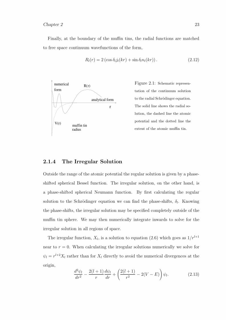
Finally, at the boundary of the muffin tins, the radial functions are matched
to free space continuum wavefunctions of the form,
Rl(r) = 2 (cos δljl(kr) + sin δlnl(kr)) . (2.12)
r)numerical
formR(
analytical form
V(r)muffin tinradius
r
Figure 2.1: Schematic represen-
tation of the continuum solution
to the radial Schrodinger equation.
The solid line shows the radial so-
lution, the dashed line the atomic
potential and the dotted line the
extent of the atomic muffin tin.
2.1.4 The Irregular Solution
Outside the range of the atomic potential the regular solution is given by a phase-
shifted spherical Bessel function. The irregular solution, on the other hand, is
a phase-shifted spherical Neumann function. By first calculating the regular
solution to the Schrodinger equation we can find the phase-shifts, δl. Knowing
the phase-shifts, the irregular solution may be specified completely outside of the
muffin tin sphere. We may then numerically integrate inwards to solve for the
irregular solution in all regions of space.
The irregular function, Xl, is a solution to equation (2.6) which goes as 1/rl+1
near to r = 0. When calculating the irregular solutions numerically we solve for
ψl = rl+2Xl rather than for Xl directly to avoid the numerical divergences at the
origin,
d2ψldr2
− 2(l + 1)
r
dψldr
+
(
2(l + 1)
r2− 2(V − E)
)
ψl. (2.13)

Chapter 2 24
Again, we separate this second order differential equation into a set of coupled
first order differential equations,
dψ(r)
dr= z(r) +
2(l + 1)
rψ(r) (2.14)
and,
dz(r)
dr= 2(V (r)− E)ψ(r). (2.15)
These equations may be solved numerically using, for example, the NAG routine
D02PCF.
2.1.5 The Initial States
We take the bound atomic states, φlo(r), from tabulations of Roothaan-Hartree-
Fock atomic functions by Clementi and Roetti [27] and by A D and R S McLean
[28].
The initial state binding energies, ωo, are taken from experimental tables where
available [29] or from the theoretical predictions of Clementi and Roetti otherwise.
As spin orbit coupling is not included in any other way apart from in the binding
energies we take each of the (2lo + 1) mo sub levels to be of identical form.
However, we do scale the contributions of each of the mo states according to the
ratio of the statistical weights of the sub levels. Thus, for example, the 2p3/2 is
taken to contribute twice the strength of the 2p1/2 initial state to the relevant
matrix elements.

Chapter 2 25
2.2 The Isolated Atom
2.2.1 A Real Scattering Potential
To evaluate the photoelectron flux we must first use standard perturbation theory
to calculate the photoelectron wave function. We begin by treating an isolated
atomic system in which an X-ray photon, of frequency ω, interacts with a single,
well defined, initial state. We may then write the perturbed wavefunction as,
ψ = φo(r) +Go(r, r′, ω − |ωo|)H ′(r′)φo(r
′). (2.16)
φo(r) is the electronic initial state of energy ωo and Go(r, r′, ω−|ωo|) is the Hartree
Green function for the system which is zero if ω < ωo. We have assumed that the
perturbation has been switched on adiabatically and is given, under the dipole
approximation, by,
H ′(r′) = Eor∑
p
Y1p(r)Y∗1p(ǫ), (2.17)
where Eo is the strength of the electromagnetic field of the X-ray beam and the
Ylm’s are spherical harmonics.
Using the explicit forms for the Green function (eqn.(2.3)) we can immediately
examine the form of the photoelectron wavefunction using equation (2.16). As
expected, the photoelectron wavefunction will have the form of a phase-shifted,
flux carrying, outgoing spherical wave, with an amplitude modified by the
perturbation matrix element, 〈Rl|H ′|φo〉. We are interested in the photoelectron
flux and hence the photoelectron wavefunctions far from the absorbing atom. This
simplifies matters because, at large r, we may ignore the first term in equation
(2.16) as the initial state, |φo(r)〉, will always be highly localised. Thus,
ψ =∫
Go(r, r′, ω − |ωo|)H ′(r′)φlo(r
′)Ylomo(r′)dr′,
= −∑
l,m,p
2πık
3Eoh
(1)l (kr)eıδlYlm(r)〈Y1p|Ylm|Ylomo
〉〈Rl|r|φlo〉 (2.18)

Chapter 2 26
Where k =√
2(ω − |ωo|) and we have written the initial state as the product of a
radial function, φlo(r′), and a spherical harmonic, Ylomo
(r). Using this result, the
photoelectron flux through a sphere of radius r centred on the absorbing atom
may be calculated from the standard expression
S =1
2ı
∫
(
ψ∗dψ
dr− ψ
dψ∗
dr
)
r2dr. (2.19)
Then, substituting for the wavefunction from equation (2.18) we find that,
S =k2E2
o
4ı
∑
l
h(2)l
dh(1)l
dr− h
(1)l
dh(2)l
dr
r2|〈Rl|r|φlo〉|2
×∑
m,p,q
16π2
9Y1p(ǫ)Y
∗1q(ǫ)
∫
YlmYlomoY1pdr
∫
YlmYlomoY1qdr. (2.20)
To obtain the contribution to the flux from a given initial state of angular
momentum lo we must sum over the degenerate mo sub levels of the initial state,
multiplying by 2 to account for spin degeneracy. By summing over mo it is also
possible to simplify the above equation using a result from Brink and Satchler [30].
The integrals over spherical harmonics may be written in terms of the Wigner-3j
coefficients,
∫
YlmYLpYlomodr=
(
(2l + 1)(2L+ 1)(2l + 1)
4π
) 1
2
l L lo
m p mo
l L lo
0 0 0
. (2.21)
In equation (2.20) we have two integrals over the spherical harmonics. Thus,
noting that the Wigner-3j coefficients may be cyclically permuted, we can apply
one of the orthogonality relations of Brink and Satchler [30],
∑
mom
l L lo
m p mo
l L′ lo
m q mo
=1
(2L+ 1)δLL′δpq. (2.22)
In equation (2.20) L = L′ = 1. Then, using the addition theorem [31] to write
∑1m=−1 Y1M(q)Y ∗
1M(q) = 3/(4π), we have that,
S =k2E2
o
8ı
∑
l
h(2)l
dh(1)l
dr− h
(1)l
dh(2)l
dr
r2|〈Rl|r|φlo〉|2
l 1 lo
0 0 0
2
. (2.23)

Chapter 2 27
The Wigner-3j coefficient in equation (2.23) is only non zero if l = lo ± 1. Also,
we may rewrite the Wronskian of the spherical Hankel functions using a relation
from Abramowitz and Stegun [32],
h(2)l
dh(1)l
dr− h
(1)l
dh(2)l
dr=
2ı
kr2. (2.24)
Then, equation (2.23) for the photoelectron flux becomes,
S =k
6(Eo)
2∑
l
A(l, lo)|〈Rl|r|φlo〉|2, (2.25)
where the angle factor A(l, lo) is defined as,
A(l, lo) = lo + 1 l = lo + 1
= lo l = lo − 1
= 0 l 6= lo ± 1. (2.26)
This result for the flux through a sphere centred on the absorbing atom is also
equal to the rate of photon absorption and as such may be easily related to
the total X-ray absorption coefficient, µo(ω). The X-ray absorption coefficient is
defined as the rate of absorption of photon energy divided by the rate of energy
transport in the X-ray beam, µ = 8πωS/cE2o . In deriving equation (2.25) we
have assumed a fully occupied no, lo orbital. To obtain the contribution from a
partially occupied initial state we must multiply by the number of electrons in
the state n(no,lo) divided by 2(2lo + 1). We must then sum over all the occupied
initial states to obtain the total contribution to the X-ray absorption coefficient,
µo(ω) =2πkω
3c
∑
no,lo
n(no,lo)
2lo + 1
∑
l
A(l, lo)|〈Rl|r|φlo〉|2. (2.27)
This simple formula gives the standard result for the X-ray absorption
coefficient of an isolated atom under the dipole approximation [33]. Energy
conservation is contained in the wavenumber of the final state, k =√
2(ω − |ωo|)
whilst the sum over initial states gives each absorption edge in turn as ω becomes
larger than |ωo|.

Chapter 2 28
2.2.2 A Complex Scattering Potential
1st Order Calculation
In the presence of an entirely real scattering potential equation (2.25) gives
the photoelectron flux through the elastic scattering channel. When inelastic
scattering events are introduced via an imaginary part to the exchange and
correlation potential, VXC(r), result (2.25) can be viewed as the total flux through
all open scattering channels. The magnitude of the photoelectron flux through
the elastic channel (the only photoelectrons which contribute to the EXAFS) may
then be examined by treating the imaginary part of the potential as a perturbation
on the Green function. The complex exchange and correlation potential is written
as the sum of its real and imaginary parts,
VXC(ω, r) = VR(ω, r)− ıVI(ω, r). (2.28)
In calculating the perturbed G we take the radial wavefunctions Rl(kr) to
be solutions of the Schrodinger equation in the presence of the real part of the
exchange and correlation potential so that in equation (2.1) we must replace
VXC by its real part, VR(ω, r). Then, writing the photoelectron Green function in
terms of a perturbation series to first order in the imaginary part of the potential,
VI , we have that,
G1(r, r′) = Go(r, r
′)− ıGo(r, r1)VI(r1)Go(r1, r′), (2.29)
where the ω labels have been suppressed and we have taken it as given that the
Green function and the exchange and correlation potential are evaluated at an
energy of ω − |ωo|. Substituting the perturbation expansion for Go(r, r′), into
equation (2.16) we may write the photoelectron wavefunction in the presence of
the complex potential at large r as,

Chapter 2 29
ψ ={∫
Go(r, r′)H ′(r′)φlo(r
′)Ylomo(r′)dr′
−ı∫
Go(r, r1)VI(r1)Go(r1, r′)H ′(r′)φlo(r
′)Ylomo(r′)dr1dr
′}
, (2.30)
where the Green function Go(r, r′) has r′ < rmt and r > rmt whilst Go(r1, r
′) has
both r1 and r′ inside the muffin tin. We assume that r1 > r′ as the initial state,
|φlo〉 will always be highly localised whilst the imaginary potential, VI is zero
toward the centre of the atom. This means that the double integral in equation
(2.30) will only be significant in the regions where r1 > r′. Also, within the muffin
tin approximation, VI is spherically symmetric so that the angular integrals over
the directions of r1 simply reduce to the orthogonality integrals for the spherical
harmonics.
Taking the appropriate relations between r, r′ and r1 we can write the
perturbed Green function (eqn.(2.29)) as,
G1(r, r′) = −ık
∑
l,m
eıδlh(1)l (kr)Y ∗
lm(r)Rl(kr′)Ylm(r
′)×{
1− 1
2〈Rl|VI |Rl − iXl〉
}
. (2.31)
The perturbed Green function has the same functional form as Go, it is merely
multiplied by a factor 1− 12〈Rl|VI |Rl− iXl〉. We can use result (2.31) to calculate
a perturbed wavefunction. This may then be substituted into equation (2.19) to
obtain a result for the photoelectron flux through the elastic scattering channel.
The integrals are the same as in the previous section, thus, again summing over
the degenerate mo sub levels of the initial state we find that, to first order in VI ,
the elastically scattered flux becomes,
S =kE2
o
6
∑
no,lo
n(no,lo)
2(2lo + 1)
∑
l
A(l, lo)|〈Rl|r|φlo〉|2(1− k〈Rl|VI |Rl〉). (2.32)
As expected the photoelectron flux through the elastic channel in the presence of
the complex potential is less than the total flux through all open channels given

Chapter 2 30
by equation (2.25). Also, the irregular solution to the Schrodinger equation does
not contribute to 1st order in VI . Equation (2.32) is easily related to the elastic
contribution to the X-ray absorption coefficient. From equation (2.32) the loss
of elastically scattered photoelectron flux as the photoelectron propagates out
through the central atom potential is obviously given by,
Al = 1− k〈Rl|VI |Rl〉, (2.33)
to first order in the imaginary part of the potential. The amplitude of each
contribution to the elastically scattered flux and hence the elastic contribution to
the X-ray absorption coefficient is obviously edge dependent. It also depends on
the angular momentum of the photoelectron final state, with the l = lo + 1 and
l = lo − 1 having different values. For K-edges of course we need only consider
the l = 1 final state.
2nd Order Calculation
We can also calculate the elastic photoelectron flux for an isolated atom to second
order in VI . To 2nd order the perturbed Green function is given by,
G2(r, r′) = Go(r, r
′) − ıGo(r, r1)VI(r1)Go(r1, r′)
+ Go(r, r1)VI(r1)Go(r1, r2)VI(r2)Go(r2, r′). (2.34)
To obtain the relevant photoelectron wavefunction far from the scattering atom
we need to set r > r′ > rmt. Also VI only exists inside the muffin tin, so r1 and r2
must be less than rmt. Finally the initial states will again be highly localised as
we are dealing with X-ray absorption by the deep core orbitals, for example the
1s orbital for K-edge absorption. Then, as VI is zero close to the nucleus we can
again take r1 > r′. Thus, the perturbed Green function will still have the same

Chapter 2 31
functional form as Go,
G2(r, r′) =−ık
∑
l,m
eıδlh(1)l (kr)Y ∗
lm(r)Rl(kr′)Ylm(r
′){
1− 1
2〈Rl|VI |Rl − iXl〉
+k2
4
(∫
Rl(r1)VI(r1)F (r1, r2)V (r2)[Rl(r2)− ıXl(r2)]r21r
22dr1dr2
)}
.
(2.35)
Where F (r1, r2) is simply the radial part of the unperturbed Green function and
has different forms depending on whether r1 or r2 is the larger. We can split the
double integral above into an integral over r2 between 0 and r1 and an integral
over r2 between r1 and rmt all within the integral over r1 between 0 and rmt.
Then F (r1, r2) can be written explicitly in each of the two integrals. Also we can
replace∫ r1o dr2 by
∫ rmt
o dr2−∫ rmt
r1dr2. Then, collecting together like terms we find
that the second order part of G2 is given by,
k2
4
{
|〈Rl|VI |Rl〉|2 +∫ rmt
o
∫ rmt
r1r21r
22(Rl(r1)VIXl(r1)Rl(r2)VIXl(r2)
−Rl(r1)VIRl(r1)Xl(r2)VIXl(r2))dr1dr2 − |〈Rl|VI |Xl〉|2 + Cı}
. (2.36)
The imaginary terms that are second order in VI , denoted by Cı in equation
(2.36), will not contribute to the flux to 1st or 2nd order. As G2 has the
same functional form as Go we may easily evaluate the elastically scattered
photoelectron flux to second order in VI . The flux is the same as in equation
(2.25), it is simply multiplied by an additional l dependent term,
Al = 1− k|〈Rl|VI |Rl〉|+3
4k2|〈Rl|VI |Rl〉|2 −
1
4k2|〈Rl|VI |Xl〉|2
−1
2k2∫ rmt
o
∫ rmt
rr2r′2
(
Rl(r)VIRl(r)Xl(r′)VIXl(r
′)
+Rl(r)VIXl(r)Rl(r′)VIXl(r
′))
drdr′. (2.37)
Again, for a K-edge, only l = 1 values are allowed and thus the amplitude is a
simple multiplicative factor.

Chapter 2 32
The equation above gives the amplitude of the elastically scattered flux to
second order in the imaginary part of the potential. We can see that this will
be little different from the 1st order calculation of the amplitude (eqn.(2.33)).
The integrals over RlVIXl will be small because, as we shall see in Chapter 4,
VI is approximately constant through most of the muffin tin sphere whilst Rl
and Xl are orthogonal. To a first approximation we can estimate the strength
of the double integral over Rl(r)VIRl(r)Xl(r′)VIXl(r
′) to be about the same as
the square of the radial matrix element, |〈Rl|VI |Rl〉|2. This is because Rl and Xl
have similar magnitudes in the region toward the edge of the muffin tin sphere
where VI exists. There will therefore be some cancellation between these terms
leaving the total result for the amplitude to be modified from the 1st order result
simply by a factor of ∼ 14k2|〈Rl|VI |Rl〉|2.
2.3 The EXAFS
2.3.1 A Real Scattering Potential
To obtain a result including the fine structure we must introduce scattering atoms
into the theory. For simplicity’s sake we consider a single shell of j scattering
atoms at a distance rj from the central atom. As each atom contributes linearly
to the EXAFS we may examine each scatterer individually then sum over all the
scattering atoms in the shell to obtain the total EXAFS.
The effect of each additional scattering potential is to perturb the central atom
Green function, Go. We model this perturbation to all orders in the scattering
potential by expanding Go to first order in the T-matrix of the scattering atom,
Gs(r, r′) = Go(r, r
′) +Go(r, r1)Tj(r1, r2)Go(r2, r′). (2.38)
To obtain the total scattering Green function from a shell of scattering atoms we

Chapter 2 33
simply sum the second term above over all the j atoms in the shell.
We will use Gs to again examine the photoelectron flux far from the central
atom, this time in the presence of the scattering atoms. Thus r > r1 and r′ < r2.
In the muffin tin approximation Tj(r1, r2) only exists inside the muffin tin of
the jth scattering atom. To evaluate the integrals involving the T-matrix it is
therefore advantageous to change variables to a coordinate system centred on
this atom. We choose r1 = rj + x and r2 = rj + y. We may then expand
the wavefunctions involved in the central atom Green function in terms of zero
potential wavefunctions centred on the scattering atom using a formula from
Pendry [8],
h1l (R + x)Ylm( ˆR + x) =∑
uv
Blmuvju(kx)Yuv(x),
h2l (R + x)Ylm( ˆR + x) =∑
uv
B(2)lmuvju(kx)Yuv(x). (2.39)
The jl(kr)’s are spherical Bessel functions and the expansion matrices, Blmuv, are
given by,
Blmuv =∑
st
4πıl−u−sh1s(kR)Y∗st(R)
∫
YlmYstY∗uvdr,
B(2)lmuv =
∑
st
4πıl−u−sh2s(kR)Y∗st(R)
∫
YlmYstY∗uvdr. (2.40)
Using these results the relevant Green functions may be written as,
Go(r, r1) = −ık∑
lm
eıδlh1l (kr)Ylm(r)Y∗lm( ˆrj + x)×
(
eıδlh1l (k(rj + x)) + e−ıδlh2l (k(rj + x)))
= −ık∑
lm
eıδlh1l (kr)Ylm(r)∑
uv
ju(kx)(
eıδlBlmuv + eıδlB(2)lmuv
)
Yuv(x),
(2.41)
and,
G(r2, r′) = −ık
∑
lm
eıδl∑
uv
Blmuvju(ky)Yuv(y)Rl(kr′)Y ∗
lm(r′). (2.42)

Chapter 2 34
If we now expand the T-matrix in an angular momentum sum,
T (r1, r2) =∑
lm
tlm(x, y)Ylm(x)Y∗lm(y), (2.43)
we can immediately perform the implied integrations over x and y in equation
(2.38) using results from standard electron scattering theory. The integrals over
x and y are simply the orthogonality relations for the spherical harmonics, and,
using results from Messiah [31] we can write the integral over the T-matrix as,
∫ rmt
ojl(kx)tlm(x, y)jl(ky)x
2y2dxdy =1
4ık
[
1− e2ıδl]
. (2.44)
Then,
GTG = −ık∑
lm
∑
LM
∑
uv
h1l (kr)eıδlRL(kr
′)Ylm(r)Y∗LM(r)
1
4
[
e2ıδu − 1]
×{
B(2)∗lmuvBLMuve
ı(δl+δL) +B∗lmuvBLMuve
ı(δl−δL)}
. (2.45)
Equation (2.45) may be used to develop the exact curved wave theory of EXAFS
first derived by Gurman et al [23, 24]. To simplify the algebra however, we shall
make the so called plane wave approximation. In this approximation we assume
that the atomic separation, rj , is large and replace the spherical Hankel functions
in equation (2.40) with their asymptotic forms. Then, using the standard relations
from Brink and Satchler [30] that,
Yaα(R)Ybβ(R) =∑
c
Ycγ(R)∫
YaαYbβY∗cγdr, (2.46)
and,
Ylm(−R) = (−1)lYlm(R), (2.47)
we can write the expansion coefficients in equation (2.40) as,
Blmuv = 4πıl−u−1 1
krjeıkrjYlm(−R)Yuv(−R)
B(2)lmuv = 4πıl−u+1 1
krje−ıkrjYlm(R)Yuv(R). (2.48)

Chapter 2 35
We can substitute these results into equation (2.45) for GTG. Then, summing
over all the j scattering atoms in the single shell considered and averaging over
the angular positions of this single shell of scattering atoms we find that the
perturbed Green function again has the same functional form as Go(r, r′),
G+GTG=−ik∑
l
h1l (kr)Rl(kr′)eıδlY ∗
lm(r)Ylm(r′)
1−∑
j
i(−1)l
2kr2je2ı(krj+δl)fj(k, π)
=∑
l
h1l (kr)Rl(kr′)eıδlY ∗
lm(r)Ylm(r′)(1− Zl), (2.49)
where Zl is obviously the second term in the curly brackets and we have introduced
a result for the backscattering factor,
fj(k, π) = −2π
ık
∑
uv
(1− e2ıδl)Yuv(R)Y∗uv(−R) = |fj(k, π)|eıψ. (2.50)
We have also ignored a contribution from the forward scattering factor, fj(k, 0),
which is second order in the EXAFS.
Using equation (2.49) for G+GTG we may evaluate the photoelectron
wavefunction and hence the photoelectron flux far from the central atom. To
first order in 1/(kr2j ) we find,
S =kE2
o
6
∑
l
A(l, lo)|〈Rl|r|φlo〉|2(1 + 2Re(Zl)). (2.51)
This expression for the photoelectron flux may again be converted into a result
for the X-ray absorption coefficient. Then, substituting for Zl and for the atomic
absorption coefficient from equation (2.27), we obtain the usual result for µ(ω),
µ(ω) = µo(ω)
1 +∑
j
(−1)l
kr2j|fj(k, π)| sin(2krj + 2δl + ψ)
. (2.52)
The EXAFS function, χ(k), is defined by µ = µo(1 + χ) from equation (1.1).
Thus, in the plane wave approximation, the EXAFS is simply given by the
second term in the curly brackets in equation (2.52), χ = 2Re(Zl). This result is
equivalent to equation (1.3).

Chapter 2 36
2.3.2 A Complex Scattering Potential
In principle we could obtain a result for the EXAFS in the presence of an
imaginary potential by perturbing the Green function and the T-matrix in the
same way as in section 2.2.2. This method however, quickly becomes very complex
and cumbersome. Instead we choose to examine the effect of the imaginary
potential on the phase-shifts.
We perturb the Green function Go(r, r′) using equation (2.29). The perturbed
Green function always has the same functional form as Go whether or not r and
r′ are inside or outside the muffin tin. Using the same arguments as in section
2.2.2 we can see that, for r and r′ outside the muffin tin the Green function
will simply be multiplied by a factor (1 − 12k〈Rl|VI |Rl〉) whilst with either r or
r′ or both inside the muffin tin the perturbed Green function can be written as
Go(1− 12k〈Rl|VI |Rl − ıXl〉). We shall see later that the ı〈Rl|VI |Xl〉 term may be
ignored. However, for the moment including this term, we may rewrite equation
(2.31) for the perturbed Green function as,
G1(r, r′) = −ık
∑
l,m
eıδ′
lh(1)l (kr)Y ∗
lm(r)Rl(kr′)Ylm(r
′), (2.53)
where we have subsumed the factor (1− k2〈Rl|VI |Rl − ıXl〉) into the phase-shifts
making δl complex. In equation (2.53) δ′l is the perturbed phase-shift. To first
order,
δ′l ≈ δl −1
2〈Rl|VI |Rl − ıXl〉. (2.54)
This is of course an approximate form for the perturbed phase-shifts, however,
using this form we can reproduce equation (2.33) for the loss of flux from an
isolated atom. We therefore believe that this approximation is a good one.
Using result (2.54) for the perturbed phase-shifts we may easily calculate
the EXAFS in the presence of the imaginary potential by following the same

Chapter 2 37
derivation as in the previous section. From equation (2.51) we can see the effect
on the EXAFS of perturbing the phase-shifts. We can also calculate the elastic
contribution to the absorption coefficient. Writing the perturbed backscattering
factor as f ′j(k, π) we have,
µel = µo(1− k〈Rl|VI |Rl〉)
1 + 2Re∑
j
i(−1)l
2kr2je2ı(krj+δ
′
l)f ′j(k, π)
. (2.55)
Then, because the total absorption must be the same regardless of whether or
not there is an imaginary part to the potential we may write the total X-ray
absorption coefficient as,
µtot = µ = µel(1− χ) + µinel, (2.56)
which gives the EXAFS as,
χ = (1− 2k〈Rl|VI |Rl〉)(−1)l
kr2jsin(2krj + 2δl + ψ)|f ′
j(π)|. (2.57)
The perturbed backscattering factor may be written as,
f ′j(k, π) =
ı
2k
∑
L
(−1)L(2L+ 1)(
1− (1− k〈RL|VI |RL〉)eı(δL−〈RL|VI |XL〉))
. (2.58)
The irregular solution to the Schrodinger equation only appears in the exponential
in the above equation. It merely alters the phase of the backscattering factor,
f ′j(k, π). However, compared to the phase-shifts, the radial matrix element
〈RL|VI |XL〉 is always small. In Chapter 4 we shall see that VI is approximately
constant over much of the region of the atom. Thus, because RL and XL are
orthogonal the matrix element 〈RL|VI |XL〉 must be small. In Chapter 4 we
compare 〈RL|VI |XL〉 to the phase-shifts δL and show that, in comparison to the
phase-shifts, the radial matrix element, 〈RL|VI |XL〉, may be ignored.
Thus, in the presence of an imaginary part to the potential the EXAFS
amplitude is given to first order in VI by,
Al = 1− 2k〈Rl|VI |Rl〉∣
∣
∣
∣
∣
f ′j(π)
fj(π)
∣
∣
∣
∣
∣
. (2.59)

Chapter 2 38
This expression may be used to calculate the amplitude of the EXAFS in the
presence of an imaginary potential designed to account for the inelastic electron-
electron scatterings. In Chapter 4 we use the above equation to examine the
magnitude of the EXAFS when the Hedin-Lundqvist [9] potential is used to model
the many-electron effects of exchange and correlation. Equation (2.59) may also
be obtained by perturbing the scattering wavefunctions (eqn.(2.5)) rather than
the photoelectron wavefunction [34].
2.4 Conclusion
In this Chapter we have developed expressions for the X-ray absorption coefficient
and the EXAFS by considering the photoelectron flux produced by irradiating
an atom with a beam of X-ray photons. We have examined the effect on the
amplitude of the EXAFS and the elastically scattered flux of introducing an
effective imaginary part of the potential to describe inelastic electron-electron
scatterings. The results derived here will be used in Chapters 4 and 5 to evaluate
the X-ray absorption coefficient and the losses to the elastic photoelectron flux
caused by various types of imaginary potential.

Chapter 3
The Self-Energy and the
Dielectric Function
In this chapter we investigate some of the theory underlying the approximation
of many-electron effects in EXAFS. We begin with a short review of some of
the approximations used in many-body physics. We then discuss the role of
screening and outline the derivation of the non-local self energy operator. We
also derive expressions for the Hartree inverse dielectric function, the quantity
which defines the screening. Numerical results for the local inverse dielectric
function are calculated for both a free electron gas and an atomic system. The
results of the atomic calculation are then equated to the single electron X-ray
absorption coefficient.
3.1 Many-Body Physics
Many-body interactions play an important role in electron-electron scattering
problems such as EXAFS. Historically a great deal of effort has been put into
39

Chapter 3 40
solving the Hamiltonian for a many-electron system,
H =∑
i
[
−1
2∇2(ri) + V (ri)
]
+1
2
∑
i 6=j
1
|ri − rj|. (3.1)
For a small number of electrons it is possible to obtain a very accurate
representation of the ground state wavefunction using the configuration
interaction method [36]. However, the computational effort scales exponentially
with the size of the system [37]. Also, for excited states the computational effort
becomes large even for small systems. Thus, using the CI method for EXAFS
calculations is impractical. Instead we must approximate the ground and excited
state wavefunctions in some other fashion.
Approximate theories are usually concerned with finding a good single particle
approximation for the coulomb term. The earliest of these theories is the Hartree
approximation in which the coulomb term is replaced by an average local coulomb
potential from all the electrons. The Hartree potential is known to give reasonable
results due to a cancellation between exchange and correlation but is not accurate
enough for many applications.
An extension of the Hartree approximation, which takes into account the
fermionic nature of the electrons, is the Hartree-Fock theory where, in addition to
the local coulomb potential, there is a non-local exchange potential which reflects
the Pauli exclusion principle. The Hartree-Fock approximation works quite well
for atoms and insulating solids but is poor in conducting solids due to the neglect
of electron correlations. In the Hartree-Fock approximation only electrons of
equivalent spins are forbidden from occupying the same state. In reality, however,
the coulomb interaction between electrons will keep even electrons of opposite
spins apart. The correlations keep electrons away from each other, creating a
screening hole around each electron which significantly reduces the interaction
with the other electrons. Thus, electron-electron correlations and screening are

Chapter 3 41
important factors in the many-body problem.
The Slater Xα potential [38] was perhaps the first to make an allowance for
these effects. In this theory the exchange is approximated by the free electron
exchange calculated with a radially varying atomic charge density. Correlation
effects are then included empirically by scaling the potential with the variable
parameter α. The Slater Xα potential is known to give good results for the
ground state but works less well for excited states.
A more accurate way of approximating the coulomb interaction term is through
a non-local energy-dependent potential, the electron self-energy. The self-energy
is a quantity which can be derived systematically from many-body perturbation
theory and which contains the effects of the exchange and correlations. The
different single particle theories amount to approximating the self energy in
different ways. In its local form, the self-energy simply becomes an effective
scattering potential which can be used in the single electron formalism of existing
EXAFS theory. The self energy is, in general complex, with the imaginary part
describing the inelastic scattering of electrons.
3.2 Screening
The concept of screening is an important one in many-body physics. In a many-
electron system a given electron will not, in general, respond directly to an applied
external field. Instead the density fluctuations induced by such a field cause an
additional potential which tends to screen out some of the effects of the total
field. It is to the total field, the sum of the external and induced potentials, that
the electrons respond. In classical physics the relationship between the total field
and a static external field may be expressed in terms of a dielectric constant,
Vtot =Vextǫ. (3.2)

Chapter 3 42
In many-body physics we generalise the idea of the dielectric constant and write
the relation between the total and applied fields in terms of an inverse dielectric
function, or response function,
Vtot(r1, ω) =∫
ǫ−1(r1, r2, ω)Vext(r2, ω)dr2, (3.3)
where, in general, the applied field may be energy-dependent and the response of
the system non-local.
The inverse dielectric function serves as a single unifying concept for many of
the properties of an interacting system of electrons. Not only does it give the
response of the system to an external field but it also contains information on
both the single particle and collective modes of the energy-dependent density-
fluctuation spectrum. The inverse dielectric function is also important when it
comes to calculating such quantities as the self-energy which are obtained by
summing over all the possible coulomb interactions. The screening reduces the
effect of the coulomb interaction at long range ensuring that the series of terms
involving the interaction converge more rapidly.
In this chapter we work under the random phase approximation, also known
as the linearised time-dependent Hartree approximation. This simply means
that we assume the electrons to respond to the total field, the sum of the
applied and induced potentials, as non interacting particles. Each electron feels a
certain coulomb potential from a given electron, this potential will be screened in
some fashion due to the fluctuations in electronic density caused by the original
potential, giving a new average field. We then assume each of the remaining
electrons to behave as non interacting particles responding to the new average
potential.

Chapter 3 43
3.3 The Self-Energy
To account for the interaction between a given electron and the rest of the
electrons in the system we must generalise the notion of a local potential
and introduce a non-local time, or energy, dependent potential. This non-
local potential, known as the self-energy, contains the exchange and correlation
effects. It is, in general, complex with the imaginary part describing the inelastic
scattering between single particle states.
The full Green function for an arbitrary many-electron system may be written
in terms of the non-local, energy-dependent potential, Σ(r1, r2, ω) [9],
(ω−H(r1)− V (r1))G(r1, r2, ω)−∫
Σ(r1, r3, ω)G(r3, r2, ω)dr3 = δ(r1, r2). (3.4)
Where, V (r) is the total average potential in the system. This is the sum
of the Hartree potential plus any external field. The Hartree and Hartree-
Fock approximations for G(r1, r2, ω) are obtained from the above equation by
specifying that Σ be energy independent. To obtain the Hartree approximation
in equation (3.4) we simply set Σ = 0. Similarly, the Hartree-Fock approximation
is obtained by making the choice Σ(r1, r2) =ı2πv(r1, r2)
∫
G(r1, r2, ω)eıδωdω.
The self-energy is generally evaluated iteratively from a set of well known
integral equations, the Hedin equations [39]. Σ(r1, r2, ω) can be written in terms
of a power series involving the unscreened coulomb interaction, v(r1, r2) or in a
more rapidly converging series in terms of the dynamically screened interaction,
Wo(r1, r2, ω) =∫
ǫ−1(r1, r2, ω)v(r3, r2)dr3. (3.5)
Wo is defined in terms of the inverse dielectric function and the unscreened
coulomb interaction, v(r1, r2) = |r1 − r2|−1. Mathematically, using the screened
interaction corresponds to summing a selective set of terms in the expansion of
Σ in the unscreened interaction to infinite order. Physically we are saying that

Chapter 3 44
each electron will not respond to any external potential but rather to the total
potential in the system, the sum of the external field and any induced potential
due to the response of the system.
A result for the self-energy in the lowest order of the screened interaction is
given by Inkson [40]. This is known as the GW approximation for the self-
energy and is the simplest working approximation beyond Hartree-Fock that takes
screening into account,
Σ(r1, r2, t1 − t2) = ıWo(r1, r2, t1 − t2)Go(r1, r2, t1 − t2). (3.6)
Where Go(r1, r2, t1 − t2) is the Hartree Green function, the solution to equation
(3.4) with the self-energy set to zero. To obtain relation (3.6) in a more convenient
form we must Fourier transform it into energy space. We use the following
definition for the Fourier transform,
f(r, t) =1
(2π)4
∫
dqdωeıq·reıωtf(q, ω). (3.7)
Thus,
Σ(r1, r2, ω) =∫
e−ıω(t1−t2)Σ(r1, r2, t1 − t2)d(t1 − t2)
=ı
2π
∫
Wo(r1, r2, ω′)Go(r1, r2, ω − ω′)dω′. (3.8)
From equation (3.5) we may write Wo in Fourier transform,
Wo(q1,q2, ω) = ǫ−1(q1,q2, ω)vq2, (3.9)
where vq = 4π|q|2 and we have used the general result that,
∫
eı(q1−q2)·rdr = (2π)3δ(q1 − q2). (3.10)
Then, substituting forWo(q1,q2, ω) into equation (3.8) for the self-energy we find
that,
Σ(r1, r2, ω) =ı
(2π)7
∫
ǫ−1(q1,q2, ω′)vq2
Go(r1, r2, ω − ω′)eıq1·r1eıq2·r2dq1dq2dω′.
(3.11)

Chapter 3 45
To proceed further, explicit forms for the Hartree Green function and the inverse
dielectric function must be used. The Green function is defined in terms of the
solutions to the single electron Schrodinger equation, φm,
Go(r1, r2, ω − ω′) =∑
m
φm(r1)φ∗m(r2)
ω − ω′ −Em + ıδ sign(Em), (3.12)
where sign(Em) = −1 if Em < 0 and the one electron states are occupied, whilst
sign(Em) = 1 if Em > 0 and the one electron states are unoccupied.
In deriving a result for the self-energy we must use the time ordered response
function [9]. This is slightly different to the causal dielectric function encountered
in perturbation theory in that the two poles in ǫ−1(q1,q2, ω) are in different half
planes. We discuss the inverse dielectric function in more detail in the following
section. For the moment we simply quote it as,
ǫ−1(q1,q2, ω) = δ(q1 − q2)
+vq1
∑
n
ρno(q1)ρ∗no(q2)
{
1
ω − ωno + ıδ− 1
ω + ωno − ıδ
}
.(3.13)
where ρno(q) is the matrix element of the density operator between the exact
ground state and a many-body excited state of the system and ωno is the difference
in energy between the system in the ground state and in the ′n′th excited state.
Using the definitions of Go(r1, r2, ω−ω′) and ǫ−1(q1,q2, ω) we can immediately
perform the ω′ integral in equation (3.11) using contours. Following Inkson [40]
we add a convergence factor of e−ıω′δ to the integral and close contours in the
lower half of the complex plane. We then obtain a contribution to the self energy
from the pole in the inverse dielectric function at ω′ = ωno− ıδ and from the pole
in the Green function at ω′ = ω − Em − ıδ. The pole in the Green function only
contributes if φm(r) is an occupied state with Em < 0. Then,
Σ(r1, r2, ω) =−1
(2π)6
∫
eıq1·r1eıq2·r2vq2
{
occ∑
m
φm(r1)φ∗m(r2)ǫ
−1(q1,q2, ω − Em)
+ vq1
∑
n
Go(r1, r2, ω − ωno)ρno(q1)ρ∗no(q2)
}
dq1dq2. (3.14)

Chapter 3 46
The terms obtained from the contribution of the two poles each have a different
physical meaning.
The pole in the Green function gives rise to the dynamically screened exchange
term. This reduces to the Hartree-Fock exchange if we take the screened
interaction to be simply the bare coulomb term, Wo(r1, r2) = v(r1, r2). The
screened exchange term is much better behaved than the normal Hartree-Fock
exchange which is known to give unphysical results for the density of states in
solids.
The pole in ǫ−1(q, ω) produces a term which can be associated with the
coulomb hole and which describes the electron-electron correlation. Classically
the coulomb hole has a simple physical interpretation. Electrons will correlate
their motion so as to screen out the electric field at large distances. In a
uniform electron gas each electron will be surrounded by a hole in the electronic
density which contains an equal and opposite charge. Thus at large distances the
coulombic effects of each electron with its surrounding hole are negligible.
r
n(r) Figure 3.1: Schematic represen-
tation of the coulomb-induced hole
in the electronic density (n(r)).
Reproduced from figure 1.3 of Ink-
son [40].
Equation (3.14) is a general result for the self-energy to the lowest order in
the dynamically screened interaction, Wo(r1, r2, ω). To make this result easily
applicable to EXAFS theory it is advantageous to write Σ in a local rather
than non-local form. We shall do this in the following two chapters in which
we investigate two different approximations for the exchange and correlation

Chapter 3 47
potential.
3.4 The Inverse Dielectric Function
The result for Σ(r1, r2, ω) obviously depends on the exact form chosen for the
screening. In this section we shall examine two forms in particular for the
inverse dielectric function. We derive expressions for the response function within
the Hartree approximation and calculate numerical results for the local inverse
dielectric function in an atomic system and for a uniform electron gas. The
calculation of the inverse dielectric function in a free electron gas is standard
and can be found in, for example, March and Jones [41], and Pines [42]. We
outline the standard derivation then apply the free electron gas relations within a
local density formalism to calculate the response function for systems of varying
charge density. This is the form of the inverse dielectric function used in the
Hedin-Lundqvist calculation of the self-energy in Chapter 4.
To our knowledge a calculation of ǫ−1(q, ω) using atomic wavefunctions has not
been performed, although an atomic dielectric function is used, at least implicitly,
in the work on complex potentials by Beni, Lee and Platzman [18].
Results for the dielectric function, especially those pertaining to a uniform
electron gas, are usually evaluated using perturbation theory (see for example,
Ziman [43], Pines [42], Nozieres [44]). This approach gives rise to the causal or
retarded response function. However, when evaluating the self-energy we must
use the time ordered inverse dielectric function [9]. Both response functions are
equal for positive energies but the time ordered function is an even function of
the energy whilst the retarded dielectric function has an even real part and an
odd imaginary part.
Hedin and Lundqvist [9] define the time ordered inverse dielectric function in

Chapter 3 48
terms of a response function, R(r1, r2, ω),
ǫ−1(r1, r2, ω) = δ(r1 − r2) +∫
dr3v(r1, r3)R(r3, r2, ω). (3.15)
The response function is given by,
R(r1, r2, ω) =∑
n
ρno(r1)ρ∗no(r2)
[
1
ω − ωno + ıδ− 1
ω + ωno − ıδ
]
, (3.16)
where,
ρno(r) = 〈ΦNo (ra..rN)|ρ(r)|ΨNn (ra...rN )〉. (3.17)
|ΦNo (ra..rN)〉 and |ΨNn (ra...rN)〉 are the exact N-body ground and excited states
for the system whilst ωno = ωn − ωo is the difference between the excited and
ground state energies. ρ(r) is the density operator. If we assume the electrons to
be point particles then the density operator may be simply written as,
ρ(r) =∑
i
δ(r− ri), (3.18)
or, in Fourier transform as,
ρ(q) =∑
i
e−ıq·ri, (3.19)
where the sum over i runs over all the electronic coordinates.
In section 3.3 we used a result for the inverse dielectric function in q and ω space.
Equation (3.13) is simply obtained by substituting for the response function into
equation (3.15) and Fourier transforming. Equation (3.13) is a general result for
the time ordered response function. In order to calculate it numerically we must
make some simplifying approximations. First, we assume the exact ground state
and excited state wavefunctions to be Hartree products of single electron orbitals,
|ΦNo 〉 =N∏
i=1
|φi(ri)〉
|ΨNn 〉 = |ψn(rj)〉
N∏
i 6=j|φi(rj)〉, (3.20)

Chapter 3 49
where the |φj(rj)〉’s are bound single electron orbitals and |ψn(rj)〉 is an excited
single electron state. In the Hartree approximation, the only many-body excited
states which can be reached are those with at most a single electron in an excited
state. Also, in the Hartree approximation, each electron is identifiable, thus,
choosing the electron to be excited to have a particular radial coordinate, rj, and
noting that the initial and final state wavefunctions are orthogonal we may write
the matrix element of the density operator as,
ρno(q) = 〈Φo(ra..rN)|∑
i
eıq·ri|Ψn(ra...rN)〉
= 〈φo(r)|ρq|ψn(r)〉, (3.21)
where ρq = exp(−ıq · r).
Thus, substituting this result into equation (3.13) for the inverse dielectric
function we find that the Hartree inverse dielectric function is given by,
ǫ−1(q1,q2, ω) = δ(q1 − q2) + vq1
∑
n
〈φo(r)|ρq1|ψn(r)〉〈ψn(r)|ρ∗q2
|φo(r))〉
×{
1
ω − ωno + ıδ− 1
ω + ωno − ıδ
}
. (3.22)
3.4.1 The Local Inverse Dielectric Function
Most calculations assume the inverse dielectric function to be local. This is
equivalent to simply ignoring the off diagonal elements in ǫ−1(q1,q2, ω). In a
uniform electron gas this approximation is, of course, exact, as the system is
translationally invariant.
Taking the diagonal elements of equation (3.22), the local inverse dielectric
function is found to be,
ǫ−1(q, ω) = 1+vq∑
n
|〈ψn(r)|ρ∗q|φo(r)〉|2{
1
ω − ωno + ıδ− 1
ω + ωno − ıδ
}
. (3.23)

Chapter 3 50
It is instructive to examine the real and imaginary parts of the above equation
separately. With the help of the formal identity,
limδ→0
1
x± ıδ= P
(
1
x
)
∓ ıπδ(x), (3.24)
we find that the real and the imaginary parts of the inverse dielectric function
are given by,
Re ǫ−1(q, ω) = 1 + vq∑
n
|〈ψn|ρ∗q|φo〉|2{
2ωnoω2 − ω2
no
}
, (3.25)
Im ǫ−1(q, ω) = −πvq∑
n
|〈ψn|ρ∗q|φo〉|2 {δ(ω − ωno)− δ(ω + ωno)} . (3.26)
The real part of ǫ−1(q, ω) describes polarisation processes in phase with the
external field whilst the imaginary part represents the out of phase part and
is related to the transfer of energy between parts of the system.
Equations (3.25) and (3.26) can be used to calculate the Hartree inverse
dielectric function in a number of different systems. We shall begin by outlining
the derivation in a free electron gas.
3.4.2 Free Electron Gas Calculation of ǫ−1(q, ω)
In the uniform electron gas the electronic wavefunctions are simply plane waves,
|φo(r)〉 = exp(ık · r),
|ψn(r)〉 = exp(ıκ · r). (3.27)
Substituting these states into the result for the local inverse dielectric function
we obtain the result that,
ǫ−1(qω) = 1 + vq∑
κ
∣
∣
∣
∣
∫
e−ıκ·r exp(ıq · r)eık·rdr∣
∣
∣
∣
2
×{
1
ω − ωκ + ωk + ıδ− 1
ω + ωκ − ωk − ıδ
}
. (3.28)

Chapter 3 51
The radial integral gives a delta function, δ(q + k − κ), which removes the sum
over final states, κ. Equation (3.28) is the contribution to the inverse dielectric
function from a single initial state only. The total inverse dielectric function is
obtained by summing over all the occupied plane wave initial states in the uniform
electron gas. We ensure that no unoccupied states are included by multiplying
the summation term by the Fermi occupation function, nk,
ǫ−1(qω) = 1 + vq∑
k
nk
{
1
ω + ωk − ωk+q + ıδ− 1
ω + ωk+q − ωk + ıδ
}
. (3.29)
To obtain the standard Lindhard form from equation (3.29) we must change
summation variables in the first term on the right hand side. We initially replace
k by k′ = k+q, then switching between k’ and -k’ in the infinite summation and
remembering that the occupation number and state energies must be independent
of the sign of the wave vector we can write,
ǫ−1(qω) = 1 + vq∑
k
nk+q − nk
ω + ωk+q − ωk + ıδ. (3.30)
This result is equivalent to the first order expansion of the Lindhard result for
ǫ(q, ω) [9]. In equation (3.30) ǫ−1(qω) is identically equal to one unless |k| > kf
and |k+ q| < kf or |k| < kf and |k+ q| < kf . Contributions to the summation
term only arise from excitations across the Fermi surface.
In equations (3.30) and (3.29) the sum of k may be replaced by an integral
dk/(2π)3. The integral in equation (3.29) is actually easiest to perform and may
be evaluated analytically to produce a result first obtained by Lindhard [45]. The
Lindhard form is, however, too complex to be of use in most practical situations
and is therefore usually approximated in some form or other.
One commonly used approximation is the single plasmon pole (SPP) form of
Hedin and Lundqvist [9],
ǫ−1(q, ω) = 1 +ω2p
2ωq
[
1
ω − ωq + ıδ− 1
ω + ωq − ıδ
]
. (3.31)

Chapter 3 52
In equation (3.31) ωp is the plasma frequency, given by ω2p = 4πn where the
electron density n = k3f/3π2 in a uniform electron gas. The plasma oscillation
frequency at a wave vector q is denoted by ωq. This can be obtained from the real
part of the Lindhard expression (eqn.(3.29)). In the high frequency limit we can
expand the real part of equation (3.29) to second order in (ωk+q −ωq)2/ω2. This
gives an expression which may be integrated and compared to the real part of the
SPP form for ǫ−1 to obtain an expression for ωq. Hedin and Lundqvist [9] use a
q dependent plasmon frequency with a slightly different numerical coefficient for
the q2 term than that obtained from the Lindhard formula,
ω2q = ω2
p +1
3q2kf
2 +1
4q4, (3.32)
At large q, ωq approaches the free particle limit of 12q2 whilst, in the small
wavelength limit, ωq reduces to ωp so that equation (3.31) reproduces the familiar
Drude relation for the optical dielectric function,
ǫ−1(0ω) = 1 +ω2p
ω2 − ω2p
. (3.33)
The imaginary part of the SPP inverse dielectric function for positive
frequencies is modelled using a single delta function. This gives a sharp
plasmon like absorption for all q but contains no contribution from particle-hole
excitations. The single plasmon pole form does, however, satisfy the same sum
rule [9] as the Lindhard inverse dielectric function. Thus, in the single plasmon
pole approximation we have assumed that all the weight in Im ǫ−1 resides in the
plasmon excitations. This is strictly true in the long wavelength limit. Also, in
the small q limit, the real part of the SPP response function and the full Lindhard
dielectric function are almost identical although at shorter wavelengths the two
forms begin to diverge.

Chapter 3 53
3.4.3 LDA of an Average Single Plasmon Pole ǫ−1(q, ω).
In the local density approximation (LDA) it is assumed that an atomic system
may be described solely in terms of its electronic density. Each volume element
of the atom is taken to respond to the total field as if it were part of an infinite
uniform electron gas of the same density. In this way we may apply homogeneous
electron gas relations locally simply by replacing the constant charge density, n,
with a radially varying function n(r). Thus, within the LDA, we can calculate
ǫ−1(q, ω) as a function of r for a particular atom, provided we know how the
charge density varies radially within that atom.
In the local density approximation both the plasma frequency, ωp, and ωq are
functions of r. We invoke the usual muffin tin approximation in which the charge
density is taken to be spherically symmetric. Thus, after spherically averaging
both the local plasma frequency and the charge density, we find we can write
the ωp in terms of the radial atomic wavefunctions, φi(r), ω2p(r) =
∑
i |φi(r)|2.
Using this result we can calculate an inverse SPP dielectric function which is
dependent on q, r and ω. Averaging this function over r will then produce an
LDA calculation of ǫ−1(q, ω) directly comparable to the atomic calculation and
to experiment.
For the imaginary part of ǫ−1(q, ω) we have,
Im ǫ−1(q, ω) =∫
drIm ǫ−1(q, ω, r)
=∫
4πr2drπω2
p(r)
2ωq(r)δ (ω − ωq(r)) , (3.34)
where we have substituted for Im ǫ−1(q, ω r) using the imaginary part of equation
(3.31) for positive frequencies and normalised to unit volume. Then, rewriting
the delta function using a standard result from Messiah [31],
δ (ω − ωq(r)) =
[
dωq(r)
dr
]−1
δ(r − rq), (3.35)

Chapter 3 54
it follows that,
Im ǫ−1(q, ω) = 2π2∫
r2ω2p(r)
ω
[
dωq(r)
dr
]−1
δ(r − rq)dr, (3.36)
where rq is the radius at which the q dependent plasma frequency is equal to the
frequency of the perturbation, ω. Equation (3.36) gives an expression describing
ǫ−1(q, ω) in a system of varying atomic density obtained obtained using the free
electron gas relations and the LDA. Using an atomic charge density to describe
ωp we can directly compare equation (3.36) to a more sophisticated atomic
calculation and to experiment.
3.4.4 Atomic Calculation of ǫ−1(q, ω)
The Imaginary Part
We wish to calculate the imaginary part of the inverse dielectric function for
an atomic system which we assume to be initially in the ground state. In this
case the energy difference between final and initial states, ωno, will always be
positive and hence the second of the delta functions in equation (3.26) will give
no contribution to Im ǫ−1(qω). It is also well known that continuum transitions
are much more likely than those into bound states [12], thus, in the sum over
excited states, |ψn〉, we concentrate only on propagating states in the continuum.
This enables us to replace the sum over final states by an integral over the free
electron density of states in the usual fashion. We may rewrite equation (3.26)
as,
Im ǫ−1(q, ω) = − πvq(2π)3
∫
dk|〈ψ(k, r)|ρ∗q|φo(r)〉|2δ(
ω − |ωo| −1
2k2)
. (3.37)
Equation (3.37) gives the contribution to the imaginary part of the dielectric
function from a single initial state. The total imaginary part of the dielectric

Chapter 3 55
function for a particular atomic system is therefore obtained by summing the
right hand side of equation (3.37) over all the occupied initial states.
As in the previous chapter, we write the continuum final states as a sum
of phase-shifted radial solutions to the Schrodinger equation multiplied by the
relevant spherical harmonics (eqn.(2.5)). This enables us to perform the angular
part of the k integral in equation (3.37) immediately,
Im ǫ−1(q, ω) =1
2
∑
i ,lf ,mf ,
∫
|〈RlfYlfmf(r)|ρ∗q|φi(r)〉|2
vqkδ(k′ − k)k′2dk′. (3.38)
In writing the above equation we have taken advantage of the orthogonality
relation of the spherical harmonics and have again used a standard result from
Messiah [31] to correctly evaluate the strength of the delta function,
δ(
ω − |ωo| −1
2k′2)
= −1
kδ(k′ − k), (3.39)
where, k =√
2(ω − |ωo|). Then
Im ǫ−1(q, ω) =1
2vqk
∑
i ,lf ,mf
|〈RlfYlfmf|ρ∗q|φi〉|2. (3.40)
To evaluate the matrix element in equation (3.40) we must now consider the
explicit forms of the initial state, |φi(r)〉, and the density operator, ρ∗q.
It is well known that a bound atomic orbital may be written as the product of
a radial wavefunction and a spherical harmonic. We can also expand the density
operator, ρ∗q, in terms of spherical harmonics using a standard result from Pendry
[8]. From equation (3.19) we have,
ρ∗q = exp(ıq · r) =∑
LM
4πıLjL(qr)YLM(q)Y ∗LM(r). (3.41)
In this formulation it is more natural to rewrite the sum over occupied atomic
orbitals as a sum over no, lo and mo quantum numbers. Then, multiplying by a

Chapter 3 56
factor of 2 to account for spin degeneracy, it follows that Im ǫ−1(qω) is given by,
Im ǫ−1(q, ω) =64π3k
q2∑
no
∑
lomo
∑
lfmf
∑
LM
∑
L′M ′
ı(L−L′)〈Rlf (r)|jL(qr)|φlo(r)〉 ×
〈φlo(r)|jL′(qr)|Rlf (r)〉〈Ylfmf|Y ∗LM |Ylomo
〉〈Ylomo|YL′M ′ |Ylfmf
〉 ×
YLM(q)Y ∗L′M ′(q). (3.42)
Again we can simplify the above equation by using a relation from Brink and
Satchler [30] to write the integrals over the spherical harmonics in terms of
Wigner-3j coefficients (eqn.(2.21)). Then noting that the Wigner-3j’s may be
cyclically permuted we can apply the orthogonality relation, equation (2.22).
Finally the addition theorem [31] may be used to rid equation (3.42) of the
YLM(q)′s. Then, as expected, we find the imaginary part of the dielectric function
to be independent of the direction of polarisation of the perturbation.
Im ǫ−1(q, ω) =4πk
q2∑
no
∑
lo,L,lf
|〈Rlf (r)|jL(qr)|φlo(r)〉|2 ×
(2lf + 1)(2L+ 1)(2lo + 1)
lf L lo
0 0 0
2
. (3.43)
This is the contribution to Im ǫ(q, ω) from a single atom consisting of fully
occupied states only. To calculate the actual atomic imaginary part of ǫ−1(q, ω) we
must multiply equation (3.43) by the number of electrons in each atomic orbital,
n(no,lo), divided by the number of electrons in a full atomic orbital, 2(2lo + 1).
Then,
Im ǫ−1(q, ω) =2πk
q2∑
no
∑
lo,L,lf
n(no,lo)
∣
∣
∣
∣
∫
r2Rlf (r)jL(qr)φlo(r)dr
∣
∣
∣
∣
2
×
(2lf + 1)(2L+ 1)
lf L lo
0 0 0
2
. (3.44)
As L increases the first maximum in the Bessel function in equation (3.44)
moves further out from the centre of the atom consequently reducing the

Chapter 3 57
magnitude of the radial matrix element at high angular momenta. The Wigner
3-j coefficients also tend to decrease as L increases [30]. Numerically we therefore
find that the L sum can be converged using a maximum angular momentum of
20 at the energies investigated. We set the condition of convergence to be that
the contribution from two subsequent angular momentum states be less than 1%
of the total contribution to Im ǫ−1(q, ω).
The real part
Once the imaginary part of ǫ−1(q ω) has been evaluated it is a simple matter to
calculate the real part using the Kramers-Kronig relation,
Re ǫ−1(q, ω) = 1 +1
π
∫ ∞
−ωo
dωkoIm ǫ−1i (q, ωko)
{
2ωkoω2 − ω2
ko
}
, (3.45)
where ωko =12k2 + |ωo|.
3.4.5 The X-ray Absorption Coefficient
Small q Limit Of ǫ−1(qω)
At low q the frequency and wavevector dependent dielectric function may be
related to the X-ray absorption coefficient, µo(ω). In the small q limit the density
operator may be expanded in a power series. Then, on use of the addition
theorem, ρ∗q becomes,
ρ∗q = exp(ıq · r) ≈ 1 + ıqr cosα = 1 + ıqrP1(cosα)
= 1 + ıqr4π
3
1∑
M=−1
Y1M(q)Y ∗1M(r). (3.46)
Substituting this expression into equation (3.40) for the imaginary part of
the dielectric function we can sum over all initial states to obtain the total
Im ǫ−1(q, ω). Then, remembering that the initial and final photoelectron states

Chapter 3 58
are orthogonal we find,
limq→0
Im ǫ−1(q, ω) =2
3πk
∑
no,lo,lf
n(nolo)|〈Rlf |r|φlo〉|2(2lf + 1)
lf 1 lo
0 0 0
2
. (3.47)
We have again used the orthogonality relations of the Wigner-3j coefficients and
the addition theorem for spherical harmonics. As in Chapter 2, the Wigner-3j
coefficient in equation (3.47) is only non zero if lf = lo±1. Thus, writing out the
3j coefficients explicitly we find that the imaginary part of the dielectric function
is given by,
Im ǫ−1(0, ω) =2
3πk
∑
no,lo
n(nolo)
2lo + 1
{
|〈Rlo+1|r|φlo〉|2(lo + 1) + |〈Rlo−1|r|φlo〉|2lo}
.
(3.48)
The q = 0 imaginary part of the dielectric function found within an atomic
calculation is related to µ(ω) by,
µo(ω) =ω
cIm ǫ−1(0ω), (3.49)
where c is the speed of light in vacuo. Thus substituting for Im ǫ−1(0ω) from
equation (3.48) we obtain a result for the absorption coefficient identical to
equation (2.27).
3.5 Results
We are now at a stage where the various forms for the inverse dielectric function
may be evaluated numerically. In this chapter we approximate the atomic
potential with the sum of the Hartree potential and the Slater Xα exchange.
In equation (2.1) we approximate VXC(r) with VXα(r) where [38],
VXα = −3
2α
(
3n(r)
π
)1
3
. (3.50)

Chapter 3 59
In the calculation of the dielectric function we deal with free atoms only. We do
this by extending the muffin tin radii to much larger values than those encountered
in the solid, typically around 25 atomic units. As we are treating free atoms
we can take the values of the variable parameter, α, in the free electron Slater
exchange potential from the tabulation of Schwarz [46].
3.5.1 The Small q Limit
The X-ray Absorption Coefficient
Using the various approximations discussed above we can calculate the X-ray
absorption coefficient in the atomic theory of equation (3.49), accurately and
efficiently over a wide range of energies and for all atoms in the periodic table. In
figures 3.2, and 3.3, we show a value for µ(ω) obtained from the inverse imaginary
part of the dielectric function plotted against energy. The absorption coefficient
does not show the complexity expected from a full band structure calculation
but compares well to the tabulated results of Veigele [47]. Veigele’s tabulations
consist of experimental data above X-ray energies of 1 keV and theoretical results
calculated using a computationally intensive Hartree-Fock theory below this
energy.
In figure 3.4 we compare results for the gold M edges which are known to show
an unusually slow onset. The calculation follows the shape of the experimentally
measured absorption coefficient [48] reasonably well but slightly overestimates
the speed of the cut in of the M-edge absorption. To compare with the M-edge
data from Owens et al directly we have normalised the calculated results to the
experimental results at 3 keV.

Chapter 3 60
0.1 1 10
photon energy (keV)
102
104
106
108
µ(ω
)
Figure 3.2: µ(ω) in Barns per atom plotted against energy in keV for silicon. The solid line
shows the result obtained from an atomic calculation, whilst the dotted line gives the result
calculated from the average LDA, SPP inverse dielectric function. The diamonds show Veigele’s
tabulated result [47].
Comparison With Free Electron Calculation
Figures 3.2 and 3.3 also show a result for µ(ω) calculated from the single plasmon
pole dielectric function within the local density approximation (eqn.(3.36)).
We can see that the average single plasmon pole dielectric function exhibits
the same overall energy dependence as the atomic calculation but, as we would
expect, lacks the sharp structure of the atomic calculations at the absorption
edges. This has a simple physical interpretation: In equation (3.36) there are
no contributions to the imaginary part of the response function at frequencies
corresponding to single particle excitation energies, instead each atom absorbs at
frequencies in a shell where ω is equal to the local q dependent plasma frequency.
We observe a sharp high energy cut off in the SPP dielectric function, beyond

Chapter 3 61
10−1
100
101
photon energy (keV)
102
104
106
108
µ(ω
)
Figure 3.3: µ(ω) in Barns per atom plotted against energy in keV for copper. The solid
line shows the result obtained from an atomic calculation, whilst the dotted line gives the
result calculated from the average LDA, SPP dielectric function. The diamonds show Veigele’s
tabulated result [47].
which the perturbing field cannot excite any response from the electron system.
The cut off frequency corresponds to the highest accessible local plasmon, ie. the
point of highest electron density of the atom in question.
For free atoms the single plasmon pole dielectric function does not exhibit a low
energy cut off for the simple reason that the charge density tends to fall smoothly
to zero by the edge of the extremely large muffin tins that are used. The atomic
calculation, on the other hand, does fall sharply to zero below a certain energy.
At frequencies lower than the binding energy of the most weakly bound state
there is not enough energy available to excite any electrons into the continuum,
and thus, within our approximations, we obtain no contribution to the dielectric

Chapter 3 62
2.1 2.2 2.3 2.4 2.5 2.6 2.7
photon energy (keV)
105
106
µ(ω
)
Figure 3.4: µ(ω) in Barns per atom plotted against energy in keV for the gold M-edges.
The dotted line is Veigele’s tabulated result, the diamonds with the dashed line show the
experimental data [48] whilst the solid line is the calculated result.
function.
Overall, the LDA single plasmon pole inverse dielectric function appears to
give a reasonable approximation to the q = 0 atomic inverse dielectric function,
except at high energies where the single plasmon pole result underestimates the
imaginary part of Im ǫ, and hence µ(ω).
3.5.2 q Dependence
In figure 3.5 Im ǫ−1(q, ω) is plotted against q at three separate energies: ω = 10
eV, ω = 100 eV and ω = 400 eV, for silicon. The solid curves show Im ǫ−1(q, ω)
calculated from the average LDA SPP ǫ−1. These exhibit a sharp cut off at a
q value where 13(qkf)
2 + 14q4 = ω. Beyond this q value, the charge density is
insufficiently large, anywhere in the atom, for a plasmon to be excited.

Chapter 3 63
0 2 4 6
q (atomic units)
0.001
0.01
0.1
1
10
Imε−
1(q
,ω)
Figure 3.5: Im ǫ−1(q, ω) against q at fixed energy for silicon. The solid lines are calculated
using the average LDA, SPP inverse dielectric function. The points are the results of the atomic
calculation. The solid line and the circles are calculated at ω = 10 eV, the dashed line and the
triangles at ω = 100 eV and the dotted line and the squares at ω = 400 eV.
The points in figure 3.5 show the equivalent results obtained from an atomic
calculation. These curves exhibit a peak in the same place as the free electron gas
results, at ω ∼ 12q2. As we increase ω the peak obviously moves out to a higher
q. As both the free electron gas calculation and the atomic calculation satisfy
the same sum rule the areas under the two sets of curves must be equivalent.
The presence of a peak in Im ǫ−1(q, ω) can be deduced if we consider the
contribution to the inverse dielectric function from each initial state separately.
In figure 3.6 we show the contribution to Im ǫ−1(q, ω) from the copper 4s and the
copper 3d initial states.
If we take the final states to be entirely free electron like and assume the initial
state to possess a spherical symmetry then, in equation (3.44) for the imaginary

Chapter 3 64
0 2 4 6
q (atomic units)
1e−05
0.001
0.1Im
ε−1(q
,ω)
0 2 4 6
q (atomic units)
0.001
0.01
0.1
1
Imε−
1(q
,ω)
Figure 3.6: The contribution to the imaginary part of an atomic inverse dielectric function
from a single initial state plotted as a function of q at fixed energy. The solid line is at ω = 20
eV, the dashed line at ω = 100 eV and the dotted line at ω = 400 eV. The curve on the left
shows the contribution from the copper 4s orbital, the curve on the right is the contribution
from the copper 3d orbital.
dielectric function, the relevant matrix element reduces to,
∫
r2φlo(r)jlf (kr)jlf (qr)dr. (3.51)
As the initial states will look something like the Slater form of rn exp(−αr)
[20], equation (3.51) will obviously have a sharp maximum at q = k where the
periods of the two spherical Bessel functions match. This effect can be seen in
the left hand curve of figure 3.6 where the contributions to Im ǫ−1(q, ω) from
an copper 4s state are plotted against q at various final state energies. We can
see that the maxima occur almost exactly at q =√2E, at q = 1.2, q = 2.7 and
q = 5.4 atomic units for E = 20 eV, E = 100 eV and E = 400 eV.
The high peak contribution to the total imaginary part of the dielectric function
is greater for the more weakly bound initial states. The muffin tin potential is
weaker at the outer regions of the muffin tin spheres and so it is in this area
where the final state becomes most free electron like and hence where there is
the greatest possibility of the final state and perturbation matching. However, it
is only the most weakly bound states that are significantly different from zero in

Chapter 3 65
these regions. The high q contribution from the more tightly bound states tends
to get killed in comparison.
In the right hand curve of figure 3.6 the contribution to Im ǫ−1(q, ω) from a
copper 3d initial state is plotted. The maxima in this function are much less sharp
than those seen previously and do not occur exactly at q = k. This is because of
the more complex angular dependence of the initial state. To get the same sort
of resonance effect we have to match a Bessel function of angular momentum L
with the final state of angular momentum lf = L± lo.
3.6 Conclusion
In this chapter we have derived expression for the non-local self energy, Σ(r1, r2, ω)
and for the Hartree inverse dielectric function. In its local form, Σ is equivalent
to an effective complex scattering potential, the imaginary part of which may
be used to describe losses to the EXAFS. We investigate Σ using two different
theories in later chapters.
The self-energy depends on the inverse dielectric function used. We have
calculated the local Hartree Im ǫ−1(q, ω) in an atomic system both directly and
via a uniform electron gas calculation using the local density approximation. We
have shown that the result of the atomic calculation may be equated to the X-
ray absorption coefficient in the limit as q tends to zero. This result will be used
in Chapter 7. The results obtained for the X-ray absorption coefficient agree
well with experiment and previous tabulated values [47]. The atomic dielectric
function is also used in the calculation of the Beni, Lee and Platzman polarisation
potential (Chapter 5), although in a non-local form.
The LDA, single plasmon pole Im ǫ−1(q, ω) is used in the Hedin-Lundqvist
calculation of the self-energy. We have shown that this form of the inverse

Chapter 3 66
dielectric function exhibits the same overall energy dependence as the atomic
form for Im ǫ−1(q, ω) but does not have the same sharp features at the single
particle excitation energies. The SPP dielectric function also underestimates the
screening at high ω and at high q because of the artificial cut off of Im ǫ−1 in this
theory, at the point where the charge density in the atom reaches a maximum.

Chapter 4
An Investigation of the
Hedin-Lundqvist Exchange and
Correlation Potential
In this chapter we investigate the Hedin-Lundqvist [9] (HL) form of the exchange
and correlation potential. This potential was first applied to EXAFS calculations
within the local density approximation by Lee and Beni [10] and is the potential
most commonly used today, for example in the Daresbury program EXCURV98
[14] and the equivalent American program, FEFF [49].
We begin by outlining the derivation of the HL potential from the general form
of the self-energy discussed in Chapter 3. We show the the Slater Xα potential
[38] and the Dirac-Hara exchange potential [50, 51] can be obtained as special
cases of the real part of the HL potential. The imaginary part of the HL potential
is also calculated.
The main part of the chapter is concerned with the losses to the EXAFS
produced by the HL potential. This potential was designed to model only the
extrinsic losses to the photoelectron beam, making no provision for the intrinsic
67

Chapter 4 68
losses. When data fitting using this potential one should therefore need to use a
value of s2o of about 0.7, equivalent to the values used in the original method of
EXAFS analysis (eqn.(1.3)). This is found not to be the case [34]. In this chapter
we calculate the losses generated by the HL potential using the theory discussed
in Chapter 2 and compare them to the historically used EXAFS loss factors: the
amplitude reduction factor, s2o, and a mean free path term, exp(−2rjVPI/k) (see
Chapter 1).
4.1 Calculation of the Potential
4.1.1 The Self-Energy
We start from the random phase approximation for the electron self-energy
defined in the previous chapter. Hedin and Lundqvist [9] derive an expression
for the self-energy in a uniform electron gas of density n. Lee and Beni [10] then
generalise this result to systems of varying charge density, such as atoms and
molecules, using the local density approximation (LDA).
It is easiest to apply the uniform electron gas relations to equation (3.11). In
the uniform electron gas the electronic wavefunctions are plane waves and all the
properties of the system must be translationally invariant. In equation (3.11) the
self-energy and Go are therefore functions of r1 − r2 only. Then, taking the local
form of the inverse dielectric function and Fourier transforming we have that,
Σ(k, w) =ı
(2π)4
∫
vqǫ−1(q, ω′)Go(k− q, ω − ω′)dω′dq. (4.1)
Where Go(k, ω) is the Hartree Green function in Fourier transform,
Go(k, ω) = (ω − Ek + ıδ sign(Ek − Ef))−1, (4.2)
and Ef is the Fermi energy.

Chapter 4 69
As in Chapter 3, we can perform the integral above using contours. Closing
contours in the lower half plane we obtain a contribution from the pole in Go
from occupied states only and a contribution from a pole in the inverse dielectric
function. To obtain the Hedin-Lundqvist result for the self-energy we must use
the single plasmon pole form for the inverse dielectric function (eqn.(3.31)). Then,
Σ(k, ω) =−1
(2π)3
∫
dq
{
nk−qvqǫ−1(q, ω − Ek−q)−
vqω2p
2ωqGo(k− q, ω − ωq)
}
,
(4.3)
Where nk−q is the occupancy of the state with wavevector k − q. If we ignore
the screening, ie. take ǫ−1(q, ω) = 1 in equation (4.1), we remove the 2nd term
from the equation above and Σ reduces to the Hartree Fock exchange potential
in the uniform electron gas,
ΣHF (k) =∫
nk−qvqdq
= −kfπ
[
1 +k2f − k2
2kkflog
∣
∣
∣
∣
∣
kf + k
kf − k
∣
∣
∣
∣
∣
]
, (4.4)
When applied under the local density approximation, in which the Fermi
wavevector becomes position dependent, equation (4.4) gives the Dirac-Hara
[50, 51] approximation to the exchange potential. This is another potential which
is commonly used in EXAFS calculations. The Dirac-Hara self-energy is known to
give good photoelectron phase-shifts [52, 53] but, as it is an entirely real potential,
it obviously does not account for inelastic scattering events in the same way as
the HL potential. The Dirac-Hara potential is also closely related to the Slater
Xα exchange (eqn.(3.50)). Taking k = kf in the above equation we obtain the
Kohn-Sham approximation to the Xα exchange which is equivalent to setting
α = 23in equation (3.50). We can also obtain an average free electron exchange
potential by summing equation (4.4) over all occupied states and then dividing

Chapter 4 70
by the total number of electrons,
VXα(k) =2
(2π)3n
∫
nkΣHF (k)dk
= −3
2
(
kfπ
)
= −3
2
(
3n
π
)
1
3
. (4.5)
The integral has been performed with the help of the computational mathematics
software, Maple. n is the number of electrons per unit volume and we have
assumed the system to be non-magnetic and have therefore treated opposite spins
equivalently. Equation (4.5) is simply the Xα exchange with a value of α = 1.
In this chapter we are mostly concerned with the inelastic scatterings of the
photoelectron. These are described by the imaginary part of equation (4.3),
ImΣ(k, ω) =ω2p
(4π)2
∫ vqωq
[nk−qδ(Ek−q − ω − ωq)
−(1− nk−q)δ(Ek−q − ω + ωq)] dq. (4.6)
Within the single plasmon pole approximation we can see that we obtain
contributions to the imaginary part of the electron self-energy from two types
of process. The 2nd term in equation (4.6) describes the absorption of electrons
of frequency ω from the system. Electrons with initial energy ω drop into an
empty state of wavevector k−q resulting in the emission of a plasmon of energy
ωq. The first term in equation (4.6) adds electrons of frequency ω into the system.
Electrons initially in a state of energy Ek−q absorb a plasmon and are excited
into the electronic state of frequency ω.
4.1.2 The Exchange and Correlation Potential within the
LDA
The relation for the electron self-energy given above applies within an electron
gas of uniform density. We may, however, modify this result so that it applies to

Chapter 4 71
real, inhomogeneous, materials by using the local density approximation. In this
approximation the assumed constant density is replaced by a spatially varying
function. As the electronic density, and hence the total potential, vary with r
the kinetic energy at the Fermi level, 12k2f , must also vary radially so that the
thermodynamic Fermi energy, Ef remains constant. Then,
1
2k2f(r) = Vo(r) + Ef + Σ, (4.7)
where Vo(r) is the electronic potential and Σ is the electron self-energy. In order
to avoid self consistency problems we follow Lee and Beni [10] and assume that the
self-energy is small compared to Vo(r) so that we may neglect Σ in the equation
above. The energy of the incident electron, ω, will also vary locally. If we take
the electron to have an energy Ei far from the scattering potential then,
ω =1
2k2(r) = Ei − Ef +
1
2k2f(r)
= Ei + Vo(r). (4.8)
As both k and ω vary with position in the local density approximation we may
write the electron self-energy as a function of r, and Ei, the energy of the electron
far from the scattering potential,
Σ(k, w) → Σ(
k(r),1
2k2(r)
)
→ V (r, Ei). (4.9)
In this case the self-energy reduces to a one body, r-dependent potential, the
exchange and correlation potential.
By substituting ω − Ek−q as ω′ = kqx − 12q2 where x is the angle between
wavevectors q and k we may write the real part of the self-energy from equation
(4.3) as,
VR(r, Ei) = −1
π
∫
{
nk−q
[
1 +ω2p
2ωq
(
1
ω′ − ωq− 1
ω′ + ωq
)]
− ω2p
2ωq
1
ω′ − ωq
}
dqdx. (4.10)

Chapter 4 72
The Fermi occupation factor, nk−q limits the dx integral from x1 to 1 where,
x1 = 1 q < qmin
=1
kq(Ei +
1
2q2 −Ef ) qmin < q < qmax
= 1 q > qmax, (4.11)
where qmin = k−kf and qmax = k+kf and x1 is always greater than −1 provided
that Ei > Ef . Where x1 = 1 we obtain a zero contribution from the x integral.
This effectively limits the range of the q integral from qmin to qmax.
The x integral above may be performed analytically for all values of q. We
can evaluate the q integral analytically in the large q limit if we replace ωq by
its asymptotic value of ωq = 12q2. We therefore choose to split the q integral
into two regions. Below qc we perform the q integral numerically whilst above qc
we approximate ωq and work analytically. We then obtain the real part of the
exchange and correlation potential as,
VR(r, Ei) = − 1
2π
{
2I1 + ω2p
[
I2 + I3 +∫ qc
o
dq
2kqωqlog
∣
∣
∣
∣
∣
(12q2 + ωq + kq)2 + δ2
(12q2 − ωq − kq)2 + δ2
∣
∣
∣
∣
∣
+∫ qc
o
dq
2kqωqlog
∣
∣
∣
∣
∣
(12q2 − ωq + kqx1)
2 + δ2
(12q2 + ωq + kqx1)2 + δ2
∣
∣
∣
∣
∣
]}
. (4.12)
Where δ is an infinitesimal used to avoid numerical divergences in the integrands.
We choose the cut-off wavevector qc to be a multiple of the plasma frequency, ωp.
A value of√100ωp appears to give satisfactory results. The results for I1, I2 and
I3 are somewhat complex. They are listed in appendix A.
As r → 0 the electronic potential, Vo(r) becomes very large thus, from equations
(4.7) and (4.8) we can see that, k(r) must be very large and approximately
equal in magnitude to kf(r). Then, ignoring all the terms proportional to 1/k(r)
in equation (4.12) we find that the HL result for the exchange and correlation
potential looks very similar to the Slater exchange (Xα) potential close in towards

Chapter 4 73
the atomic nucleus,
VR(r, Ei) = −kf (r)π
. (4.13)
Equation (4.13) is obviously just the Kohn-Sham approximation to the Xα
exchange.
We evaluate the imaginary part of the self-energy in a similar fashion starting
from equation (4.6). The Fermi occupation function, nk−q, limits the x integral
from x1 to 1 whilst the factor (1− nk−q) limits the integral from −1 to x1, then,
VI(r, Ei) =ω2p
2k
∫ dq
qωq
{
∫ 1
x1δ
(
x−12q2 − ωqkq
)
dx−∫ x1
−1δ
(
x−12q2 + ωqkq
)
dx
}
.
(4.14)
For photoelectrons with energy Ei greater than the thermodynamic Fermi energy,
Ef only the second term contributes and hence,
VI(r, Ei) = −ω2p
2k
∫ qmax
o
dq
qωq
∫ x1
−1δ
(
x−12q2 + ωqkq
)
dx. (4.15)
The imaginary part of the exchange and correlation potential is only non zero
for electrons with energies greater than that needed to excite a local plasmon,
Ei −Ef > ωq. Below this energy the incident electrons are not energetic enough
to excite a plasmon and so, in the single plasmon pole approximation, inelastic
scattering events are impossible.
Using equations (4.12) and (4.15) we can calculate the real and imaginary parts
of the exchange and correlation potential as a function of r. In the next section
of this chapter we compare the real parts of the HL potential to the Dirac-Hara
potential (equation (4.4)) and the free electron Slater exchange (equation (3.50)).
We also investigate the magnitude of the inelastic scattering events modelled by
the imaginary part of the self-energy. We use VI(r, Ei) to calculate the losses
to the EXAFS signal accounted for in this formalism and compare these to
experimental data.

Chapter 4 74
4.2 Results
In this chapter we wish to investigate the HL potential for materials in the solid
state. We therefore take the muffin tin radii to be appropriately small. By
doing this we may compare directly with most EXAFS measurements and with
previous work. Also the HL potential should be more accurate for systems of
high electronic density.
4.2.1 The HL Potential
In the figure below we plot the real and imaginary parts of the HL potential
against r for Bromine at various photoelectron energies. These curves can be
compared to the original results produced by Lee and Beni [10].
0.001 0.01 0.1 1 10
r (atomic units)
−1.4
−0.9
−0.4
rVR(r
) (H
artr
ees)
0 1 2 3 4
r (atomic units)
−0.5
−0.4
−0.3
−0.2
−0.1
0
rVI(
r) (
Har
tree
s)
Figure 4.1: The real and imaginary parts of the HL potential plotted against r for Bromine
at various energies. The left hand curve shows rVR(r) at k = 8 a.u. (dot-dash curve), at k = 4
a.u. (dotted curve) and at k = 0.5 a.u. (solid line). The Slater Xα exchange with α = 0.8 is
shown for comparison (dashed curve). The right hand graph shows rVI (r) at k = 7 a.u. (solid
line), k = 5 a.u. (short dashed line) and k = 3 a.u. (long dashed line).
The real part of the exchange and correlation potential decreases with
increasing energy. This is reasonable. A fast moving photoelectron will have
much less chance of interacting with the bound electrons than a low energy

Chapter 4 75
photoelectron. At low energies and at small r the real part of the HL potential
looks like the Slater Xα exchange as expected. The real and imaginary parts to
the potential are discontinuous at the edges of the muffin tin spheres where we
have truncated the atomic density.
The imaginary part of the HL potential is zero at small r. In this region of
high electronic density the incident photoelectron is insufficiently energetic to
excite a plasmon. As soon as the density falls sufficiently for plasmons to be
excited VI cuts in almost immediately to its maximum value. At larger incident
photoelectron energies VI obviously cuts in at lower radii, however, for large Ei
the imaginary part of the potential is generally smaller in the outer regions of the
atomic muffin tins.
0 1 2
r (atomic units)
−0.65
−0.45
−0.25
−0.05
VI(
r) (
har
tree
s)
Figure 4.2: The imaginary part of the HL potential in Hartrees, at k = 8 atomic units.
Calculated for silicon (solid line), copper (dotted line) and silver (dashed line).
Figure 4.2 shows the imaginary part of the HL potential calculated for three
elements: silicon, copper and silver. The imaginary part of the HL potential

Chapter 4 76
looks very similar for these very different elements. The electron mean free paths
for these elements will therefore also be very similar as has long been assumed
experimentally. The radius at which the HL potential cuts in moves slightly
outward as we go up in atomic number. This is because the electron density
is larger close to the nucleus for elements with higher atomic numbers. The
corresponding plasmon excitation frequency is therefore higher and so we have to
move further out from the centre of the atom before it becomes possible to excite
a plasmon with a photoelectron of given energy.
In figure 4.3 we compare the Slater Xα exchange to the real part of the
HL potential and the energy-dependent Hara exchange potential calculated for
copper. The curve on the left gives the comparison at a photoelectron wavevector
of k = 0.5 atomic units whilst the graph on the right is at k = 8 a.u.
0.001 0.01 0.1 1 10
r (atomic units)
−1.4
−0.9
−0.4
rVR(r
) (H
artr
ees)
0.001 0.01 0.1 1 10
r (atomic units)
−1.4
−0.9
−0.4
rVR(r
) (H
artr
ees)
Figure 4.3: Comparison between the Dirac-Hara potential (solid line), the HL potential (short
dashed line) and the Slater exchange with α = 0.8 (long dashed line) at k = 0.5 atomic units
(left hand graph) and k = 8 atomic units (right hand graph). Calculated for copper.
At low photoelectron energies all three potentials look reasonably similar. As
we move to higher energies the Dirac-Hara and HL potentials decrease reflecting
the fact that high energy electrons will ”see” less of the atomic potential. The

Chapter 4 77
Slater Xα potential is on the other hand, energy independent. The Dirac-Hara
potential falls off faster than real part of the HL potential with energy. In the
outer regions of the atom, where the electron density is lower and the screening
less important, the Dirac-Hara potential appears too small. We know that the
HL potential gives good results for the EXAFS, it is the potential used in both
the Daresbury EXAFS code [14] and its American equivalent [49]. However, the
Dirac-Hara potential also gives good phase-shifts for EXAFS purposes [52]. In
fact Chou et al [53] state that the Dirac-Hara is better than the corresponding
real part to the HL potential. EXAFS calculations mostly deal with high
photoelectron energies. At these energies the scattering from the atomic core
dominates and the details of the atomic potential in the low electron density
regions at the edges of the muffin tins becomes less important.
4.2.2 The Average Potential
We can calculate the average imaginary part of the HL potential simply from,
VAV G(k) =3
r3mt
∫ rmt
oVI(r, k)r
2dr. (4.16)
In figure 4.4 we plot the average imaginary part of the potential against k for
copper. The imaginary part of the potential has an average value of approximately
4.6 eV over most of the range of energy appropriate to EXAFS data analysis. This
is close to the canonical value of 4 eV generally used to account for the extrinsic
losses in LEED calculations for example [8]. The average imaginary part of the
HL potential is also very similar for all atoms. This is a consequence of describing
the atoms as shells of varying electron density.
Figure 4.4 also shows that the average potential falls off with increasing photon
energy above the edge. This can also be deduced from equation (4.15). We only

Chapter 4 78
0 2 4 6 8
k (atomic units)
−0.2
−0.15
−0.1
−0.05
0
VA
VG(k
) (h
artr
ees)
Figure 4.4: The average imaginary part of the HL potential plotted as a function of k for
copper.
obtain a contribution from the delta function if,
∣
∣
∣
∣
∣
12q2 + ωqkq
∣
∣
∣
∣
∣
< 1. (4.17)
Taking the limit of high photoelectron energy so that k becomes very large and
12k2 >> ωp we find that we will always obtain a contribution from the delta
function provided that q < k and q > ωp/k. Then, at high k,
VI =ω2p
2
∫ k
ωp
k
dq
kqωq
=ωpk
[
1
2log
(
kqcωp
)
+ωp3q2c
]
, (4.18)
where, to a first approximation, we have approximated ωq with its low q limit
below qc and with its high q limit of 12q2 above qc. We can see that equation
(4.18) for VI will obviously go to zero as k becomes very large. VI only models
the extrinsic photoelectron scatterings and therefore this is correct.

Chapter 4 79
4.2.3 The Isolated Atom
In Chapter 2 we calculated expressions which described the flux loss from the
elastic photoelectron beam as the photoelectron propagated through a single
muffin tin. In figure 4.5 we compare the results obtained to first and second
order (eqn.(2.33) and eqn.(2.37)). In this figure, and the rest of the chapter we
treat events following a K-edge photoionisation. In this way we need only consider
the lf = 1 final state.
0 2 4 6 8
k (atomic units)
0.6
0.8
1
flu
x l
oss
Figure 4.5: The loss of flux from the elastic photoelectron beam from an isolated atom
calculated for copper. The solid line shows the result of the 1st order expression (eqn.(2.33)),
the dashed line shows the result of the second order expression (eqn.(2.37)).
The second order calculation can be used to give an estimate of the errors
involved in the first order expression for the EXAFS amplitude which we shall
examine in the next section. Over most of the energy range plotted in figure
4.5 the results of the two calculations differ by approximately 2%. To a first
approximation we can ignore inelastic events at the scattering atom and write the

Chapter 4 80
EXAFS amplitude to first order as being proportional to 1 − 2k〈R|VI |R〉. This
would give results from the EXAFS amplitudes differing by about 5% between
the first and second order calculations. This error is much smaller than the error
associated with the amplitude fitting parameters used in EXAFS data analysis.
We must also bear in mind that including higher order terms in the second order
calculation would bring the curve down toward the first order result because of
the opposing signs of the most important terms in each additional order.
0 2 4 6 8
k (atomic units)
−0.01
0
0.01
0.02
<R
l|VI|X
l>/δ
l
Figure 4.6: The matrix element 〈Rl|VI |Xl〉 divided by the phase-shift δl at l = 0 (solid line),
l = 1 (dashed line) and l = 2 (dotted line).
In Chapter 2 we stated that the radial matrix element 〈Rl|VI |Xl〉 in equation
(2.58) was small in comparison to the phase-shifts, δl. In figure 4.6 we plot
〈Rl|VI |Xl〉/δl against energy from k = 0 to 9 atomic units. We can see that for
most of the energy range investigated 〈Rl|VI |Xl〉 is much less than 1% of the
phase-shifts. The neglect of this term in the calculation of the EXAFS amplitude
(eqn.(2.59)) is therefore valid.

Chapter 4 81
4.2.4 EXAFS Amplitudes
In figure 4.7 we plot the calculated EXAFS amplitude for copper (solid line)
alongside the contribution to the EXAFS losses from inelastic processes at the
central atom (dashed line) and from the inelastic processes at the scattering atom
(dotted line).
0 2 4 6 8
k (atomic units)
0
0.2
0.4
0.6
0.8
1
Am
pli
tud
e
Figure 4.7: Calculated EXAFS amplitude for copper. The solid line shows the total result.
The dashed line gives the contribution from the central atom muffin tin whilst the dotted
line gives the contribution from the scattering atom. The diamonds are calculated using the
Daresbury program EXCURV98.
To obtain the set of data denoted by diamonds in figure 4.7 we have examined
the amplitudes of the EXAFS signals calculated using the HL and Xα potentials
respectively. EXCURV98 was used to calculate an EXAFS spectra for copper foil
using the HL potential. We refined the fit using the first shell only so that we
could easily obtain the relevant path lengths for the electron mean free path losses.
The refined fit gave a nearest neighbour distance of r1 = 2.541 ± 0.006 A a 1st

Chapter 4 82
shell coordination number of n1 = 11.3±1.5, a Fermi energy of Ef = −13.2±0.8
eV and a Debye-Waller factor of a1 = 0.016±0.002. These parameters were then
used as input to recalculate the spectra using the real Xα potential. The spectra
calculated using the Xα exchange is much larger than the best fit HL spectra as
it includes none of the losses to the photoelectron beam from inelastic scattering.
The ratio of the peak heights can be used as an approximation to the losses
given by the imaginary part of the HL potential. This data is shown by the
diamonds in figure 4.7. The results from the 1st order calculation and the
diamonds differ by an average of ∼ 8% over the whole energy range. This gives
another measure of the uncertainty in the 1st order calculation. It is smaller than
the comparable uncertainty in the EXAFS fitting parameters.
In figures 4.8, 4.9, and 4.10 we plot the EXAFS amplitude as a function of
photoelectron wavevector in atomic units.
0 2 4 6 8
k (atomic units)
0
0.5
1
Am
pli
tud
e
Figure 4.8: Calculated and best fit EXAFS reduction factors plotted against photoelectron
wavevector for silicon. The black line gives the calculated result, the solid band shows the
extent of the error in the best fit EXAFS amplitude.

Chapter 4 83
The EXAFS amplitude is calculated using equation (2.59) for three elements:
silicon, copper and silver. This is then compared to known values of the empirical
parameters, s2o(k) and e−2rj/λ(k), fitted using the real X-alpha potential for the
three elements with the data analysis program EXCURV98. The best fit values
of s2o and an effective, constant, imaginary potential, VPI , were found to be [54]
s2o = 0.72 ± 0.1 for silicon, s2o = 0.70 ± 0.1 for copper, and s2o = 0.67 ± 0.15 for
silver. The VPI values used were: −4.0 ± 0.2 eV for silicon, −4.0 ± 0.2 eV for
copper and −6.3± 0.2 eV for silver where the quoted uncertainties are 2σ errors.
The amplitude mean free path term is calculated from the constant imaginary
potential, VPI , using the standard relation λ(k) = k/VPI . In the figures the solid
band shows the product of the fitted vales of s2o and e−2rj/λ(k) within the limit of
experimental error whilst the black line gives the calculated EXAFS amplitude
(eqn.(2.59)). Below a k of about 2 atomic units the historically used EXAFS
reduction parameters exhibit unphysical behaviour. Using a constant imaginary
part to the potential we obtain a zero mean free path at low k and hence an
EXAFS amplitude of zero. This is obviously incorrect as, below, the minimum
electron excitation energy in the system there cannot be any inelastic scatterings
and hence the EXAFS amplitudes should be one.
At low X-ray energies above the edge the calculated amplitude is unity. This
is correct. At low energies the photoelectron is insufficiently energetic to excite a
plasmon anywhere in the atomic muffin tin. The energy at which the amplitude
begins to deviate from unity corresponds to the plasmon frequency in the region of
low electronic density toward the edge of the muffin tin. In an atomic calculation
this cut-in energy would be that of the most weakly bound atomic orbital. The
rapid cut-in of the amplitude reduction is a feature of the HL potential. This
occurs because the majority of the imaginary part of the HL potential comes
from the region of almost constant electronic density toward the edge of the

Chapter 4 84
0 2 4 6 8
k (atomic units)
0
0.2
0.4
0.6
0.8
1
Am
pli
tud
e
Figure 4.9: Calculated and best fit EXAFS reduction factors plotted against photoelectron
wavevector for copper. The black line gives the calculated result, the solid band shows the
extent of the error in the best fit EXAFS amplitude.
muffin tin spheres.
At high k the HL potential overestimates the EXAFS amplitudes. The HL
potential models the extrinsic loss effects and so, like the mean free path term
it will disappear at high energies. From Figures 4.8, 4.9 and 4.10 it is clear that
the calculated amplitudes are still increasing at k = 8 a.u. The HL potential
itself varies as 1/k at large k, and, as the radial wavefunctions, Rl(kr), are also
proportional to 1/k at high energies, the EXAFS amplitudes given by the HL
potential will obviously tend to unity. However, using the sudden approximation
we can show that the intrinsic loss parameter, and hence the total amplitude
reduction, should tend to a constant value of about 0.7 at high photoelectron
energies (see Chapter 6). This is because the HL potential does not include a
contribution from the core hole.
The losses obtained from the HL potential agree reasonably well with the total

Chapter 4 85
0 2 4 6 8
k (atomic units)
0
0.2
0.4
0.6
0.8
1
Am
pli
tud
e
Figure 4.10: Calculated and best fit EXAFS reduction factors plotted against photoelectron
wavevector for silver. The black line gives the calculated result, the solid band shows the extent
of the error in the best fit EXAFS amplitude.
reduction given by the semi-empirical reduction parameters. The HL potential
must therefore overestimate the losses produced by the mean free path effects
alone. Over the range of a typical EXAFS spectrum, 2 to 7 atomic units,
the calculated reduction parameters lie within the error range of the best fit
experimental data. The correlation between the calculations and the fitted
empirical parameters can be measured in this region using the R-factor,
R =
∑ |Aexpt − Atheory|∑ |Aexpt|
× 100%. (4.19)
We find R = 4.9% for silicon, R = 6.5% for copper, and R = 10.4% for silver.
These uncertainties are much lower than those observed in the best fit parameters
for the various elements: 15.5% for silicon, 16.1% for copper and 24.4% for silver,
which suggests that the reduction given by the HL potential is equivalent to that
produced by the semi-empirical reduction parameters.

Chapter 4 86
15 25 35 45 55 65
Atomic number
0.5
1
1.5
s o2
Figure 4.11: The amplitude reduction factor obtained by fitting EXAFS spectra using the HL
potential with the Daresbury program EXCURV98. Plotted as a function of atomic number.
EXCURV98 was also used to fit values for the adjustable parameter, s2o,
using the HL potential. We found values of s2o(k) = 0.92 ± 0.10 for silicon,
s2o(k) = 1.05 ± 0.05 for copper and s2o(k) = 1.02 ± 0.05 for silver. These values
are all consistent with unity which suggests that additional amplitude fitting
parameters should not be used when data fitting using the HL potential. It
would appear that the HL potential gives extremely good results for EXAFS
calculations, albeit accidentally.
Fitting the amplitude reduction parameter for a number of elements we obtain
the points shown in figure 4.11. These points exhibit some scatter but are
generally much larger than the values of s2o which we would expect to obtain
using the Xα potential and a mean free path term. We therefore conclude that
the HL potential significantly overestimates the extrinsic losses to the EXAFS
amplitude. Empirically, the HL potential includes some of the contribution from

Chapter 4 87
the intrinsic loss events.
To summarise, the HL potential was designed to model the extrinsic loss
effects. However, using equation (2.59) or the Daresbury program EXCURV98 we
find that the imaginary part of the HL potential significantly overestimates the
losses produced by the extrinsic effects alone. Instead it seems to, qualitatively,
reproduce the total losses to the EXAFS amplitude even though the average
imaginary part is consistent with the constant potential of −4 eV obtained from
LEED experiments. The reason for this is the shape of the imaginary part of
the HL potential. The average value would correctly account for the extrinsic
losses, however, the HL potential emphasises the middle and outer regions of the
muffin tin as opposed to the region near to the nucleus where r2Rl(r) is small
anyway and therefore overestimates the losses. This can be immediately seen
from a calculation of the energy-dependent mean free path obtained from the HL
potential.
In figure 4.12 we plot the mean free paths for aluminium obtained from three
different calculations and compare to data reproduced from Penn [55]. In an
isolated atom the loss of photoelectron flux is related to the mean free path by
exp(−rmt/λ(k)) where λ is the relevant mean free path for flux. Equating this
expression to equation (2.33) for the flux loss caused by the imaginary part of
the HL potential we can immediately obtain an expression for the mean free path
given by the HL potential,
λHL(k) =−rmt
log(1 + k〈Rl|VI |Rl〉). (4.20)
In terms of a constant imaginary potential the flux mean free path can be written
λ(k) = k2VPI
.
In figure 4.12 we can see that the HL potential gives a mean free path that
is much shorter than that found experimentally. The average part of the HL

Chapter 4 88
0 2 4 6 8 10
k (atomic units)
0
10
20
30
40
λ(k
) (a
tom
ic u
nit
s)
Figure 4.12: The energy-dependent mean free path in atomic units plotted against k in
atomic units for aluminium. The solid line is that obtained from the imaginary part of the HL
potential. The dashed line is calculated from the average imaginary part of the HL potential,
the dotted line is that given by a constant imaginary potential of −4 eV and the diamonds are
data reproduced from Penn [55].
potential, however, reproduces the experimental results to much better accuracy
and gives magnitudes for the mean free path comparable to those obtained from
a constant imaginary potential of -4 eV. The mean free path for both the HL
potential and the average HL potential goes to infinity below the minimum
plasmon excitation energy where no inelastic scattering events are possible.
To emphasise this result, the radially dependent HL potential is incorrect. It
predicts values for the mean free path which are much too small. The average
HL potential, on the other hand, gives values which agree tolerably well with
experiment. It is the constant density, r independent, imaginary part of the HL
potential (equivalent to the average HL potential) that, for example, Rehr et al
[5] have claimed to give good agreement with the experimentally found mean free

Chapter 4 89
paths.
4.3 Conclusion
In this chapter we have outlined the derivation of the Hedin-Lundqvist exchange
and correlation potential commonly used for EXAFS calculations. The real and
imaginary parts of the potential have been calculated within the local density
approximation for a number of different elements. The losses to the EXAFS
given by the imaginary part of the potential were then examined using the method
described in Chapter 2.
We find that the HL potential overestimates the losses to the EXAFS due to the
finite photoelectron mean free path alone. However, it happens to give excellent
agreement with the total experimental losses in the energy range of most EXAFS
data analysis.
Empirically the HL potential seems to account for all of the losses to the
EXAFS amplitudes. It should therefore not be necessary to use the amplitude
fitting parameters s2o and VPI when data fitting using this potential. However
the HL potential is ’merely a phenomenological model that happens to work
for the EXAFS’ [26], by no means does it rigorously describe all the processes
contributing to the inelastic scattering of the photoelectron. Effectively the HL
potential underestimates the mean free path of the photoelectron leading to some
ad hoc inclusion of the intrinsic effects. It is therefore possible that some further
fitting of the amplitude using the variable parameters will be necessary when
using the HL potential for EXAFS calculations.
Chapter 5
An Investigation of the Beni, Lee
and Platzman Polarisation
Potential
In the previous chapter we have shown that the HL potential, whilst giving
reasonable agreement with EXAFS experiment, significantly overestimates the
extrinsic photoelectron losses that it was designed to model. This may be
because the HL potential does not include single electron excitations except by
an appropriate weighting of the plasmons. The excitations of core levels and
relatively localised states, such as the noble metal d-bands, will, however, exhibit
atom-like behaviour. Thus modelling these excitations as plasmons will not, in
general, be appropriate.
In 1976 Beni, Lee and Platzman (BLP) [18] derived a complex energy-
dependent potential (the polarisation potential) which explicitly includes the one
electron excitations although it neglects the plasmon excitations. This potential
was used to calculate the scattering from the copper d-band and appeared to give
reasonable results. In this chapter we investigate the BLP form of the polarisation
90

Chapter 5 91
potential without the simplifying approximations used by Beni, Lee and Platzman
in an attempt to see if it will correct for the failings with the Hedin-Lundqvist
form and if it may be considered as a viable alternative thereof.
BLP [18] derive their form for the polarisation potential by examining the
atomic scattering factor, f(η). In the first Born approximation the atomic
scattering factor is simply the Fourier transform of an effective scattering
potential. However, f(η) summed to all orders of scattering may also be evaluated
in terms of the exact many-body wavefunctions of the system and the coulomb
interaction potential. BLP obtain their form for the polarisation potential by
equating the two results for f(η). This method is explained in more detail
in appendix B, however, in this chapter we show that the BLP form for the
potential may also be derived using the GW formalism discussed in Chapter 3. By
developing the polarisation potential via this method we can see why the potential
describes correlation effects but does not include the electronic exchange, as stated
by Lee and Beni [10].
We must start from the general form for the non-local self-energy derived in
Chapter 3 (eqn.(3.14)). First we Fourier transform this result into energy and
momentum space,
Σ(ki,kf , ω) =∫
e−ıki·r1e−ıkf ·r2Σ(r1, r2, ω)dr1dr2. (5.1)
As we are again interested only in elastic scattering we chose the initial and final
state photoelectron wavevectors to be ki and kf with |kf|=|ki| and kf−ki = η. To
obtain the BLP potential we must evaluate the density operator matrix elements
ρno(q) within the Hartree approximation using bound atomic orbitals as the initial
states, and continuum wavefunctions, ψn(r), for the final states as in Chapter 3.
Finally, we need to approximate G(r1, r2, ω − ωno) as Go(km, ω − ωno), the free
electron Greens function. ie. the photoelectron states in the Greens function

Chapter 5 92
must be assumed to be plane waves. This immediately removes the dynamically
screened exchange term from the result for the self-energy. As we are dealing with
an atomic system (the Cu 3d orbital) there are no occupied plane wave states and
thus the sum over occupied states in equation (3.14) will not contribute to the
final result. We are therefore left with a complex scattering potential containing
only the contribution from the coulomb hole. This describes the electron-electron
correlation. Thus, from equation (3.14), we have,
Σ(ki,kf , ω) = − 1
(2π)9
∫
dr1dr2dq1dq2dkmeı(q1−ki+km)·r1eı(q2−ki+km)·r2
× vq1vq2
∑
n
ρno(q1)ρ∗no(q2)
ω − 12k2m − ωno + ıδ
, (5.2)
where ωno = ωn−ωo and we have removed the sum over initial states because we
are only dealing with a single copper 3d orbital. Ideally we should sum over the
initial states of all the electrons available to scatter the incoming photoelectron.
Beni, Lee and Platzman, however, only calculate the contribution to f2 from the
3d orbital in copper arguing that the scattering from this weakly bound state will
dominate over that from the more deeply bound core orbitals.
The r1 and r2 integrals in equation (5.2) simply give 2π3δ(km − ki − q) and
2π3δ(q2 − η + q) respectively. To obtain the standard form for the polarisation
potential we have written q = −q1. Then, assuming the initial photoelectron
energy, far from the atom, to be ω = 12k2i we find that,
Σ(η,1
2k2i ) = −4
π
∫
dq∑
n
〈φo |eıq·r |ψn〉〈ψn |eı(η−q)·r |φo〉q2 | q− η | 2(q2 + 2qkix+ 2ωno − ıδ)
. (5.3)
We have written x = cos θ, where θ is the angle between the wavevectors ki
and q. As f(η) = 12πΣ(η, 1
2k2i ) equation (5.3) gives an identical result to that
produced by BLP. Equation (5.3) is therefore simply the Fourier transform of an
effective complex scattering potential. This potential may be added to the Hartree
potential to give a one-body approximation to the full interaction potential.

Chapter 5 93
Intuitively we would expect the polarisation potential to be more physically
accurate than the equivalent HL form for the potential. The BLP form explicitly
includes one electron excitations from bound states into the continuum because
of its inclusion of the atomic single electron form of the inverse dielectric function
(eqn.(3.22)). The BLP potential also includes inelastic effects because, whenever
an inelastic scattering channel opens up at ω− 12k2m−ωno, the energy denominator
in equation (5.2) goes to zero and we obtain an imaginary contribution to the
scattering factor.
5.1 Calculation of the Polarisation Potential
We can now use equation (5.3) to evaluate an r dependent polarisation potential
without the simplifying approximations used by Beni, Lee and Platzman.
In their original paper, BLP calculate the second Born approximation to
the scattering factor, and hence the polarisation potential, using a spherically
symmetric initial state for the copper 3d electrons and orthogonalised plane
waves for the continuum final state wavefunctions. For the sake of computational
efficiency they also split the range of the q integral, replacing the integrand in
equation (5.3) with approximate forms valid in the limits of q ≪ η and q ≫ η.
We calculate Σ(η, 12k2i ) using full Clementi wavefunctions for the initial 3d state
and exact numerical results for the final state wavefunctions. We are also able
to perform the integrals in equation (5.3) without approximating the integrand.
However, because we wish to calculate the polarisation potential for copper metal,
we encounter a problem in that the copper 3d orbital extends beyond the edge of
the atomic muffin tin sphere. We deal with this problem in a fashion suggested by
Pendry [8]. We assume that the influence of the neighbouring atoms is to push
the overlapping wavefunction back inside its own muffin tin sphere. Although

Chapter 5 94
a particular muffin tin may lose charge because its own functions overlap the
muffin tin boundary it will also gain charge from the overlap of wavefunctions from
neighbouring atoms. This is taken into account by truncating the 3d wavefunction
at the muffin tin boundary and increasing its amplitude within to give the correct
number of electrons in the level.
Equation (5.3) can be immediately Fourier transformed into r space. We change
variable from η to k = q − η, then, rewriting the sum over final states as an
integral over the free electron density of states, we find that,
Σ(r,1
2k2i ) = −4
π
∑
mo
∫
dqdkdkneı(k−q)·r 〈φo |eıq·r |ψn〉〈ψn |eı(η−q)·r |φo〉
q2k2(q2 + 2qkix+ 2ωno − ıδ), (5.4)
where kn is the wavevector of the excited state ψn and we have summed over
the contribution from each of the degenerate mo initial states. The continuum
wavefunctions are defined as in equation (2.5) so that the angular parts of the
kn integral may be easily performed. Then, expanding the exponentials in the
matrix elements in an angular momentum sum (eqn.(3.41)), and replacing the r
dependent initial states with φlo(r)Ylomo(r), we may write,
Σ(r,1
2k2i ) = − 4
π3
∑
lfmf ,mo
∑
L,M
L′,M′
∫
dqdkk2ndkneı(k−q)·rYLM(q)YL′M ′(k)
q2k2(q2 + 2qkix+ 2ωno − ıδ)〈Rlf |jL(qr′) |φlo〉
× 〈φlo |jL′(kr′′) |Rlf 〉∫
dr′YlmYLMYlomo
∫
dr′′YlomoYL′M ′Ylm. (5.5)
The angular integrals are identical to those encountered in Chapters 2 and 3.
They may be expressed in terms of the Wigner-3j coefficients [30]. Within the
muffin tin approximation we are also only interested in spherically symmetric
potentials, thus, expanding the remaining exponentials and averaging Σ(r, 12k2i )
over the directions of r, we have,
Σ(r,1
2k2i ) = − 2
π3
∑
l,lo,L
Al,lo,L
∫
k2ndkndqdkdx
q2 + 2qkix+ 2ωno − ıδjL(qr)jL(kr)
× 〈Rlf |jL(qr′) |φlo〉〈φlo |jL(kr′′) |Rlf 〉, (5.6)

Chapter 5 95
where ωn = 12k2n and,
Alf ,lo,L = (2lf + 1)(2lo + 1)(2L+ 1)
lf lo L
0 0 0
2
. (5.7)
The dx integral in equation (5.6) may be written as,
∫ 1
−1
dx
q2 + 2ωno + 2qkix− ıδ= log
∣
∣
∣
∣
∣
q2 + 2ωno + 2qkiq2 + 2ωno − 2qki
∣
∣
∣
∣
∣
+ ıπ∫ 1
−1dxδ(q2 + 2ωno + 2qkix). (5.8)
The dk integral in equation (5.6) may also be performed analytically. We
can use the relation, jl(kr) =(
π2kr
) 1
2 JL+ 1
2
(kr) to express the integral over the
spherical Bessel functions in terms of the hypergeometric function, 2F1 [56],
∫ ∞
0jL(kr)jL(kr
′)dk =π
2(rr′)1
2
∫
1
kJL+ 1
2
(kr)JL+ 1
2
(kr′)dk
=π
2(rr′)1
2
(rr′)L+1
2
2(r + r′)2L+1(L+ 12)2F1
{
L+1
2, (L+ 1); 2L+ 2;
4rr′
(r + r′)2
}
. (5.9)
This expression may be simplified using a standard result for 2F1 taken from
’Formulas and Theorems for the Special Functions of Mathematical Physics’ [57],
2F1(a, a+1
2; 2a+ 1; z2) = 22a[1 + (1− z2)
1
2 ]−2a. (5.10)
We obtain different results for the integral over the spherical Bessel functions
depending on whether r or r′ is the larger.
∫ ∞
ojL(kr)jL(kr
′)dk =π
4(
L+ 12
)fL(r, r′), (5.11)
where,
fL(r, r′) =
(
r′
r
)L1
rr ≥ r′
=(
r
r′
)L 1
r′r′ ≥ r. (5.12)

Chapter 5 96
We can now substitute relations (5.8) and (5.11) into equation (5.6) to obtain the
final results for the real and imaginary parts of the BLP polarisation potential.
Multiplying by a factor of two to account for spin degeneracy in our (presumed
full) copper d-band we have,
VR(r,1
2k2i ) = − 2
π3
∑
lf ,lo,L
Alf ,lo,L
L+ 12
∫ ∞
0dq∫ ∞
0dknk
2n log
∣
∣
∣
∣
∣
q2 + k2n + 2 |ωo | +2qkiq2 + 2k2n + 2 |ωo | −2qk i
∣
∣
∣
∣
∣
× jL(qr)〈Rlf |fL(r, r′) |φlo〉〈φlo |jL(qr′′) |Rlf 〉 (5.13)
and,
VI(r,1
2k2i ) = − 1
2π
∑
lf ,L
Alf ,L,lo(
L+ 12
)
∫ qmax
qmin
dq∫ xmax
−1dxknjL(qr)〈Rlf |fL(r, r′) |φlo〉
× 〈φlo |jL(qr′′) |Rlf 〉δ(
kn − (−2 |ωo | −q2 − 2qkix)1
2
)
, (5.14)
where,
qmin = ki − (k2i − 2 |ωo |)1
2
qmax = ki + (k2i − 2 |ωo |)1
2
xmax = − q
2k i− |ωo |
qki. (5.15)
We have written the real part of Σ(r, 12k2i ) as VR and the imaginary part as VI .
These results can be made more general by summing over all of the no and lo
initial states and multiplying by the fractional occupancy of each state.
5.2 The Average Self-Energy
Beni, Lee and Platzman calculate a quantity they define as the imaginary part
of the electron self-energy from the 2nd Born correction to the atomic scattering
factor,
ImΣ = 2πNIImf2(0), (5.16)

Chapter 5 97
where NI is the ion density. This result is, in fact, just the self-energy at
η = 0 averaged over the volume of the solid. This is equal to the average value
of the imaginary part of the r-dependent polarisation potential and is closely
related to the imaginary part of the local inverse dielectric function (eqn.(3.23)).
Substituting for η = 0 into equation (5.3) we have,
Σ(0,1
2k2i ) = −4
π
∫
dq∑
n
| 〈ψn |eıq·r |φlo〉 |2q4(q2 + 2qkix+ 2ωno − ıδ)
. (5.17)
Thus,
ImΣ(0,1
2k2i ) = −
∫
dq4
q4∑
n
| 〈ψn |eıq·r |φlo〉 |2 δ(2ωno + q2 + 2qkix), (5.18)
where the delta function is given by,
δ(2ωno + q2 + 2qkix) = − 1
2knδ(kn − (−2 |ωo |−q2 − 2qkix)
1
2 ). (5.19)
Equation (2.5) may again be used to substitute for the continuum wavefunctions.
Then, rewriting the sum over excited states as an integral over the density of
states and summing over the degenerate mo levels of the initial 3d state we can
easily perform the angular integrals in the same manner as in the previous section.
We find that,
ImΣ(0,1
2k2i ) =
∑
L,l
∫ qmax
qmin
dq∫ xmax
−1dx
k
q2| 〈Rlf (kr) |jL(qr) |φlo(r)〉 |2 Alo,l,L,
(5.20)
where k = (−2 |ωi|−q2−2qkix)1
2 and the limits of the integrals are given by results
(5.15). Comparing this result to equation (3.44) we can see that the average value
of the polarisation potential may may expressed simply in terms of the imaginary
part of the dielectric function,
ImΣ(0,1
2k2i ) = −1
π
∫ qmax
qmin
∫ xmax
−1Im ǫ−1
3d (q,−1
2q2 − qkix)dxdq. (5.21)
The limits of the integrations are such that −12q2 − qkix > 0. In order that
we may compare our results directly with BLP we have taken Im ǫ−13d (q, ω) to

Chapter 5 98
be the contribution to the imaginary part of the dielectric function from the 3d
orbitals only. As we have already evaluated Im ǫ−1(q, ω) for a number of cases we
may easily calculate ImΣ(0, 12k2i ) as a function of the momentum of the incident
photoelectron. This is plotted in figure 5.1.
0
-0.04
-0.08
-0.12
-0.16
-0.2
1 2 3 4 5 6 7 8
ImΣ
k (atomic units)
Figure 5.1: The average imaginary part of the polarisation potential in Hartrees as a function
of incident photoelectron wavevector, where ω = 1
2k2i .
The average value of the imaginary part of the polarisation potential varies
slowly with energy over the range of incident photoelectron momenta appropriate
to the EXAFS. The average imaginary potential is zero for photoelectrons
of energy less than the binding energy of the copper 3d state, as, in this
approximation, no secondary electron excitations are possible below this energy.
ImΣ(0, 12k2i ) peaks at a value of approximately 3.8 eV. This is comparable in
size to the results obtained by BLP and agrees reasonably well with the −4 eV
magnitude for the constant imaginary part of the potential assumed in most
LEED calculations.
Chapter 5 99
5.3 Results
We can now calculate numerical results for the real and imaginary parts of the
polarisation potential using equations (5.13) and (5.14). The details of the
calculation are much the same as in Chapter 3. The copper 3d orbitals are
again approximated by the Roothaan-Hartree-Fock states tabulated by Clementi
and Roetti [27] and the regular solutions to the Schrodinger equation, Rlf (kr),
are calculated using the Runga-Kutta routine described in Chapter 2. The
calculations are performed within the muffin tin approximation of Loucks where
we have assumed the spherical potential to be the sum of the Hartree potential and
the Slater exchange. As we are treating copper metal rather than copper atoms
we cannot use the values of the free electron exchange parameter, α, tabulated
by Schwarz [46]. Instead we set α by examining full band structure calculations.
This procedure is detailed later.
5.3.1 The Imaginary Part
We begin by calculating the imaginary part of the BLP polarisation potential.
The integrals are performed using a simple trapezium rule routine on a linear
grid where the point density may be increased until the integrals have converged.
The sum over plane wave angular momenta is converged as in the calculation
of ǫ−1(q, ω). This introduces an error of ∼ ±1.0% into the final results for the
polarisation potential.
We find that our results for the imaginary part of the polarisation potential
depend critically on the details of the muffin tin potential and the magnitude of
the Fermi energy. The calculation of VI(r,12k2i ) is much more sensitive to the final
state phase-shifts, and hence the d-band occupancy, than was the calculation of
ǫ−1(q, ω). The muffin tin potential can be altered by varying the parameter α in

Chapter 5 100
the Slater exchange potential (eqn.(3.50)).
0 0.5 1 1.5 2
r (atomic units)
−10
−8
−6
−4
−2
0
VI(
r,ω
)
Figure 5.2: The imaginary part of the polarisation potential in Hartrees as a function of r
plotted at ki = 2 atomic units for a range of values of the Slater exchange parameter, α = 0
(solid curve), α = 0.25 (circles), α = 0.5 (dot-dash line), α = 0.75 (diamonds) and α = 1.0
(dashed line).
In figure 5.2 we plot VI against r for a range of values of α at ki = 2 atomic
units with a Fermi energy of zero. The potential varies over approximately a full
order of magnitude, which is clearly unacceptable. To calculate VI accurately
we should first find the real part of the polarisation potential using some self
consistent calculation then use VR to calculate the phase-shifts needed to evaluate
the imaginary part of the potential. This is, however, a time consuming and
computationally intensive procedure. We therefore attempt to approximate the
effects of exchange and correlation using the Slater exchange potential with
definite, fixed, values of α and Ef . We set the Slater exchange parameter and the
Fermi energy by using the Friedel sum rule to calculate the d-band occupancy

Chapter 5 101
in terms of the final state phase-shifts. We first fix α so that the centre of the
d-band is at an energy which agrees with band structure calculations, then set
Ef to obtain the correct occupancy.
Friedel Sum Rule
To make use of the Friedel sum rule we consider the atom interacting with the
X-ray photon to be an impurity added to the free electron continuum. The charge
on this impurity must be normalised by extra electrons within a finite distance in
such a way that the chemical Fermi energy remains unchanged at large distances
from the impurity. This leads to an additional density of states in the region of
the central atom [41],
∆N(E) =2
π
∑
l
(2l + 1)dδldE
. (5.22)
The number of electrons in a certain l state is then obtained by integrating
equation (5.22) and adding the number already present in the free electron density
of states,
N(E) =2
π
∑
l
(2l + 1)δl +2√2
3π2V E
3
2 , (5.23)
where V is the atomic volume. For the copper 3d band the impurity states
dominate over the continuum states but the presence of the continuum states
is much more important in jellium-like metals such as Aluminium. We can use
equation (5.23) to calculate the d-band occupancy from the final state phase-
shifts by setting l = 2. For copper, where the impurity states dominate the free
electron states, we will obtain a full d-band at energies where δ2 ∼ π.
In the left hand graph of figure 5.3 we plot δ2(E) against energy for α = 1.0, 0.75
and 0.5. We obtain an atomic-like d-band with α = 1.0. This has zero width
and is completely bound. α = 0.75 gives a d-band of narrow but finite width
(∼ 0.1 Hartrees). To fill the d-band given by this value of the Slater exchange

Chapter 5 102
0 0.5 1
E (Hartrees)
0
1
2
3
δ2(E
)
0.15 0.2 0.25 0.3 0.35 0.4
E (Hartrees)
0
1
2
3
δ2(E
)
Figure 5.3: copper d phase-shifts as a function of energy. In the graph on the left the dotted
line is calculated with the Slater exchange parameter, α = 0.25, the dot-dash line with α = 0.5,
the solid line with α = 0.75 and the dashed line with α = 1.0. The graph on the right shows
the d phase-shifts on an expanded scale calculated with α = 0.79 (solid line), α = 0.80 (dotted
line) α = 0.78 (dashed line).
parameter we would need to set Ef above 0.4 Hartrees as it is not until this value
that δ2 reaches its maximum value. With values of α < 0.5 we obtain extremely
broad d-bands. From figure 5.3 we can immediately see why the magnitude of the
imaginary part of the potential varies with α as it does. By setting α = 0.5, for
example, we allow the possibility of resonant transitions into unoccupied d-states
in the continuum. As there is consequently a high probability of the bound
electrons being excited by the photoelectron there must be a correspondingly
large imaginary part to the scattering potential.
The right hand plot of figure 5.3 shows the l = 2 phase-shifts against energy
on an expanded scale. Full band structure calculations reproduced by Harrison
[58] show the centre of the copper d-band to be at 0.252 Hartrees. By examining
the phase-shifts we can clearly see that we need to set α ∼ 0.79 to obtain this.
The d-band in copper is occupied up to the Fermi energy, Ef . For copper metal

Chapter 5 103
0
2
4
6
8
10
12
14
0 0.1 0.2 0.3 0.4 0.5 0.6
n(E
)
E (Hartrees)
Figure 5.4: Occupancy of the
copper d-band plotted against
energy with α = 0.79. The
horizontal solid line marks n(E) =
9.5 whilst the vertical solid line is
at E = 0.268 Hartrees.
the electron configuration will not be exactly as it would in a free atom (3d104s1)
but will probably have a character more like 3d9.54s1.5. We must therefore set
the Fermi energy so that filling the d-band up to Ef results in an occupancy of
∼ 9.5 electrons. In figure 5.4 we plot the number of electrons calculated from
equation (5.23) against the energy. A Fermi energy of Ef = 0.268 Hartrees
(7.3 eV) must be used to obtain the correct occupancy. Schwarz [46] records a
value of α = 0.706 for a free atom of copper. Using this value of α we would
need to set Ef to an unfeasibly high level in order to obtain the correct d-band
occupancy. Figure 5.4 also shows why the calculation is so sensitive to the value
chosen for the Fermi energy. Varying Ef by a few eV’s results in large changes to
the d-band occupancy. This in turn greatly effects the probability of exciting a
secondary electron, especially for low energy photoelectrons, where the majority
of the energetically possible excitations would be into the low lying d states if
these were unoccupied.
Numerical Results
Using the fixed values of α and Ef we can now calculate the imaginary part of
the polarisation potential for the copper d-band. In figure 5.5 we plot VI(r,12k2i )
against r for a range of incident photoelectron energies. We obtain magnitudes

Chapter 5 104
for the imaginary part of the potential which are very similar to BLP’s. However,
the energy dependence is not the same and the variation with r is slightly different
in that the BLP polarisation potential falls off faster in the outer regions of the
muffin tin spheres. These slight differences are not surprising. Both the energy
dependence and r dependence of the potential vary significantly with both α and
Ef . Also we would expect the different final states used by BLP to affect the
shape of the potential.
0 0.5 1 1.5 2
r (atomic units)
−3
−2
−1
0
VI(
r,ω
)
Figure 5.5: The imaginary part of the polarisation potential in Hartrees plotted against r at
ki = 2 (solid line), ki = 4 (dashed line) and ki = 6 atomic units (dotted line).
As we increase the energy of the incident photoelectron the imaginary part
of the potential decreases. This is as we would expect. An extremely energetic
photoelectron incident on a scattering atom will not significantly interact with the
electrons in that atom. There is therefore little probability of secondary electron
excitation and correspondingly only a small imaginary part to the polarisation
potential for high energy photoelectrons.
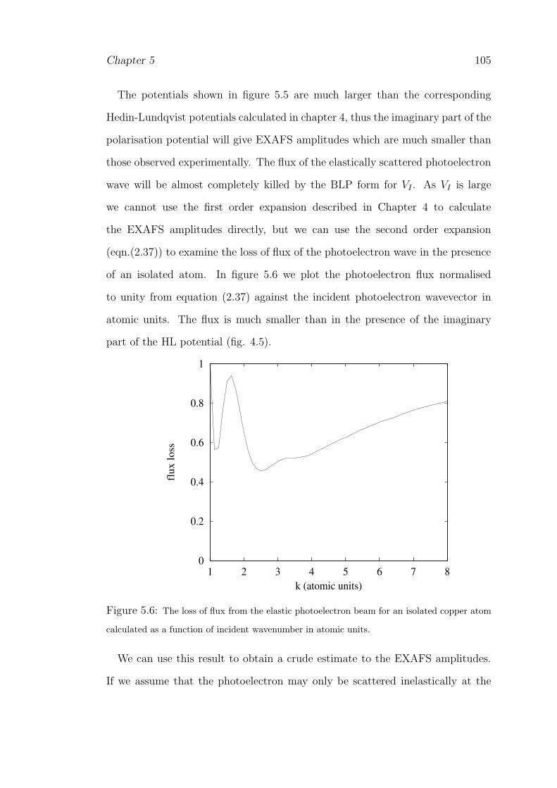
Chapter 5 105
The potentials shown in figure 5.5 are much larger than the corresponding
Hedin-Lundqvist potentials calculated in chapter 4, thus the imaginary part of the
polarisation potential will give EXAFS amplitudes which are much smaller than
those observed experimentally. The flux of the elastically scattered photoelectron
wave will be almost completely killed by the BLP form for VI . As VI is large
we cannot use the first order expansion described in Chapter 4 to calculate
the EXAFS amplitudes directly, but we can use the second order expansion
(eqn.(2.37)) to examine the loss of flux of the photoelectron wave in the presence
of an isolated atom. In figure 5.6 we plot the photoelectron flux normalised
to unity from equation (2.37) against the incident photoelectron wavevector in
atomic units. The flux is much smaller than in the presence of the imaginary
part of the HL potential (fig. 4.5).
0
0.2
0.4
0.6
0.8
1
1 2 3 4 5 6 7 8
flux l
oss
k (atomic units)
Figure 5.6: The loss of flux from the elastic photoelectron beam for an isolated copper atom
calculated as a function of incident wavenumber in atomic units.
We can use this result to obtain a crude estimate to the EXAFS amplitudes.
If we assume that the photoelectron may only be scattered inelastically at the

Chapter 5 106
central atom then the EXAFS amplitude is given by 1− 2× (1− flux loss). This
simple approximation underestimates the losses given by VI but still gives EXAFS
amplitudes much smaller then those observed experimentally. The Beni, Lee and
Platzman polarisation potential therefore greatly overestimates the strength of
the imaginary part of the potential.
Setting α and Ef from physical considerations obviously does not lead to
physically acceptable results for the imaginary part of the polarisation potential.
However the form of the calculation is such that we may fix the Fermi energy
and the Slater exchange parameter to obtain VI ’s of approximately the correct
magnitude, but only if we know what that magnitude should be before hand.
This is obviously not an acceptable situation. To improve the calculation of VI
we would therefore have to use some self-consistent procedure for which the real
part of the polarisation potential would first have to be calculated.
5.3.2 The Real Part
We can evaluate the real part of the polarisation potential using equation (5.13).
This calculation is slightly more complex than the corresponding computation of
the imaginary part of the potential. We have to be careful when performing the
kn integral because of the logarithmic divergence in the integrand, also, we cannot
integrate with respect to q or kn over the full range of the integration, but must
truncate the integral at some point. As the integrand falls off uniformly as both
kn and q become much larger than ki the integral may be safely truncated once
a point has been reached where the magnitude of the integrand is so small that
it no longer contributes to equation (5.13). Empirically we find that this point
is reached once kn and q are greater than about 5ki. The logarithmic divergence
in the integrand is also easily dealt with. We use the NAG routine D01ALF to

Chapter 5 107
perform the kn integral in the region of the singularity.
0 0.5 1 1.5 2
r (atomic units)
−15
−10
−5
0
VR(r
,ω)
Figure 5.7: The real part of the polarisation potential in Hartrees as a function of r plotted at
ki = 2 atomic units for a range of values of the Slater exchange parameter, α = 0 (solid curve),
α = 0.25 (circles), α = 0.5 (dot-dash line), α = 0.75 (diamonds) and α = 1.0 (dashed line).
In figure 5.7 we plot the calculated real part of the polarisation potential against
r for a range of values of α at an incident photoelectron wavevector of 2 atomic
units. Again, the calculated potential varies significantly with the Slater exchange
parameter and hence with the details of the band structure.
As in the calculation of VI we set α andEf to give the correct d-band occupancy.
This will give us the best obtainable real part to the polarisation potential without
the use of a self consistent calculation.
Figure 5.8 shows VR(r,12k2i ) at ki = 2, 4 and 6 atomic units. We find that the
magnitudes of the real part of the potential are similar to those calculated by
Beni, Lee and Platzman. In the left hand graph of figure 5.9 we compare the
real part of the HL potential with the sum of the Slater exchange potential and

Chapter 5 108
0 0.5 1 1.5 2
r (atomic units)
−3.5
−2.5
−1.5
−0.5
VR(r
,ω)
Figure 5.8: The real part of the polarisation potential in Hartrees as a function of r plotted
at ki = 2 atomic units (solid curve), ki = 4 (dashed curve) and ki = 6 atomic units (dotted
curve), calculated with α = 0.79.
the polarisation potential at ki = 2 and 6 atomic units. We have assumed that
the best approximation to the real part of the exchange and correlation potential
within the BLP formalism, is given by VXC(r,12k2i ) = VXα(r) + VR(r,
12k2i ). The
Hedin-Lundqvist and BLP forms for VXC exhibit similar energy and r dependence.
The BLP potential is, however, much stronger, especially close into the nucleus.
In figure 5.9 we show the phase-shifts calculated using a muffin tin potential of
VH(r) + Vxc(r,12k2i ) (where VH is the Hartree potential). These exhibit similar
behaviour to those calculated using VH(r) + VXα(r) because, as we can see from
figure 5.8 the energy-dependent polarisation potential is merely a small correction
to the Slater exchange.

Chapter 5 109
0 0.5 1 1.5 2
r (atomic units)
−3
−2.5
−2
−1.5
−1
−0.5
0rV
R(r
,ω)
0
0.5
1
1.5
2
2.5
3
3.5
0.1 0.15 0.2 0.25 0.3 0.35 0.4 0.45 0.5
δ 2
(E)
E (Hartrees)
Figure 5.9: The graph on the left shows a comparison between the real part of the HL
potential (lines) and the sum of the Slater exchange potential and the real part of the BLP
polarisation (lines with circles) potential. rV (r) in atomic units is plotted against r in atomic
units at ki = 2 (solid line and solid line with circles) and ki = 6 (dotted line and dotted line
with circles). The graph on the right shows the l = 2 phase-shift calculated as a function of
photoelectron energy using a muffin tin potential of VXC = VXα(r) + VR(r,1
2k2i ) (solid line)
and VXC = VXα (dashed line).
5.3.3 A Self-Consistent Calculation
In theory it should now be possible to calculate the real part of the polarisation
potential self-consistently. We can add the calculated VR’s to the sum of the
Hartree and Slater exchange potentials to create a new muffin tin potential. This
is then used to calculate a new set of phase-shifts which in turn can be used to
evaluate a new set of polarisation potentials. The procedure is then continued
until the calculated potential has converged. This calculation, however, becomes
progressively more difficult for each iteration. To calculate the polarisation
potential at ki = 2 atomic units after one iteration we must first calculate the
zeroth order BLP potential up to a photoelectron energy of ki = 10 atomic units.
To calculate the same potential after two iterations we would need to calculate the

Chapter 5 110
zeroth order VR(r,12k2i ) up to ki = 50 atomic units (an energy of ∼ 1400 eV) and
the 1st order potential up to ki = 10 etc. At such high energies the calculation
of the numerical final states becomes problematical. The calculations are also
too time consuming to be of practical use in EXAFS data analysis problems as
the calculation of the real part of the polarisation potential at a single initial
photoelectron energy takes about two and a half minutes. However, as VR(r,12k2i )
is small compared to VH + VXα we shall attempt to use the zeroth order results
for VR to calculate new results for the imaginary part of the potential.
0 0.5 1 1.5 2
r (atomic units)
−1
−0.8
−0.6
−0.4
−0.2
0
VI(
r,ω
)
Figure 5.10: First order calculation of the imaginary part of the polarisation potential in
Hartrees plotted as a function of r at ki = 2 (solid line), ki = 4 (dashed line) and ki = 6 (dotted
line) atomic units.
To obtain the correct band structure using a muffin tin potential of VH(r) +
VXα(r) + VR(r,12k2i ) we must set α = 0.79 and Ef = 0.272 Hartrees (7.4 eV).
Figure 5.10 shows VI(r,12k2i ) at ki = 2, 4 and 6 atomic units. The magnitudes
of VI are smaller than were found previously but are still much larger than the

Chapter 5 111
0
0.2
0.4
0.6
0.8
1
0 1 2 3 4 5 6 7 8
flux l
oss
k (atomic units)
Figure 5.11: The magnitude of the photoelectron flux as the photoelectron propagates through
an isolated muffin tin as a function of incident wavevector in atomic units. The flux is calculated
from the imaginary part of the polarisation potential using the 2nd order result (eqn. (2.37)).
corresponding values of the Hedin-Lundqvist potential. In figure 5.11 we plot
the flux of a photoelectron wave scattered by an isolated muffin tin potential
against the incident photoelectron energy. The flux is again smaller than we
would expect physically and would lead to EXAFS amplitudes much smaller
than those observed experimentally. It is possible that higher iterations of the
self-consistent calculation of the BLP potential would lead to better results for
VI , however, because of the limitations of the computer program we were not able
to test this.
5.4 Conclusion
In this chapter we have investigated the BLP form of the polarisation potential.
By developing the potential via the GW approximation we were able to show

Chapter 5 112
that the potential does not account for exchange effects but merely approximates
the electron-electron correlation. Intuitively we would expect the potential to
describe the inelastic scattering of localised states like the copper d bands more
accurately than the Hedin-Lundqvist potential because it explicitly includes one
electron excitations. However, this was not found to be the case.
In calculating the complex, energy-dependent potential we were able to
avoid many of the simplifying approximations originally used by Beni, Lee
and Platzman. We discovered that the results for the imaginary part of the
potential are extremely dependent on the values used for the Slater exchange
parameter, α, and the Fermi energy. This is because the possibility of secondary
electron excitations is greatly affected by the number of d-band states in the
continuum. We found that setting α and Ef to give the best approximation to
the band structure did not lead to physically acceptable results for VI(r,12k2i ).
The BLP form for the polarisation potential greatly overestimates the strength
of the inelastic scattering and hence significantly underestimates the EXAFS
amplitudes.
The real part of the polarisation potential was also calculated. VR(r,12k2i ) was
discovered to be small in comparison to the Slater exchange potential and gave
only a small correction to the phase-shifts. A fully self-consistent calculation of
the real part of the BLP potential was found to be computationally infeasible
but the zeroth order VR’s were used to recalculate the results for VI . The first
order imaginary potentials were found to be physically more acceptable than the
previous results but still lead to EXAFS amplitudes much smaller than observed
experimentally.
In conclusion we find that the BLP form for the polarisation potential is
completely unsuitable for EXAFS calculations. It is possible to fix the variable
parameters, α and Ef to give an imaginary part to the potential of the required

Chapter 5 113
magnitude but only by using a prior knowledge of that magnitude. Setting α
and Ef using physical constraints does not lead to acceptable values of VI and,
whilst a self-consistent calculation of VI would appear to lead to better results it
is far too time consuming to be of any practical use in EXAFS calculations. The
BLP potential therefore does not give a good description of the extrinsic inelastic
scattering of the EXAFS photoelectron.

Chapter 6
The Core hole - Photoelectron
System in the Sudden
Approximation
In this chapter we calculate the amplitude reduction factor of equation
(1.3), and hence the probability of secondary electron excitation, following a
photoabsorption event. We examine the limit of high photoelectron energy, the
so called sudden limit [19], where the time-dependent, core hole - photoelectron
system is greatly simplified. In this limit the photoelectron leaves the atom
instantaneously and the passive electrons in the atom (those not interacting
with the X-ray photon) experience a sudden change in potential corresponding
to the appearance of the core hole. This change in potential may be modelled
very simply using Slater’s rules [20]. In this fashion it is a simple matter to
evaluate the secondary excitation probabilities, and hence s2o, for all edges of all
elements. The values of the amplitude reduction factor obtained are compared to
experiment. We also calculate the probability of exciting any secondary electron
into a bound or continuum state following the photoabsorption. The continuum
114

Chapter 6 115
excitation probabilities will be needed in the following chapter. The calculation
of the amplitude reduction factor is repeated using tight binding, rather than
atomic, initial states. In this way we can determine the chemical dependence of
the amplitude reduction factor, s2o.
The probability of secondary electron excitation has been studied extensively
within the sudden approximation. However, not to our knowledge, for all
elements from an EXAFS perspective. Shake-off intensities have been calculated
in the sudden limit by, for example, Aberg [59], Carlson [11, 60] and Dyall [61]
using wavefunctions varying in complexity from single electron states to multi-
configuration Hartree Fock states. Carlson [11] examines the shake probabilities
for 15 elements across the periodic table following Beta decay in which the
nuclear charge is suddenly increased by one. This has been suggested as an
approximation for the core hole created during EXAFS, however it is a crude
one. Electrons in the same shell or in orbitals inside the photoelectron initial state
will obviously see much less of an effect from the photoionisation than electrons
in more weakly bound shells. Using Slaters recipe we can model the effect of
the core hole following a photoionisation from any edge more accurately than
with the Beta decay Z+1 approximation. In the sudden approximation the shake
probabilities are given by the monopole matrix elements between the passive
electron eigenstates in the presence and the absence of the core hole. Most of the
computational effort in the studies mentioned goes into solving for the perturbed
passive electron eigenstates (the initial states are well tabulated). By applying
Slater’s rules to model the effect of the core hole, however, the calculation of the
relaxed atomic orbitals becomes trivial.

Chapter 6 116
6.1 The Amplitude Reduction Factor
Standard, one electron, EXAFS theory (see for example equation (1.3)) includes
an amplitude reduction factor, s2o(ω), that allows for processes that contribute
to the X-ray absorption coefficient, µ(ω), but not to the EXAFS. The need for
this factor is ascribed to the possibility of multiple electron excitations at the
absorbing atom. s2o(ω) is almost always treated as a free parameter to be fixed by
reference to a standard sample [62], and is an important factor in the experimental
determination of coordination numbers. In this process it is implicitly assumed
that its value is independent of the chemical environment of the absorbing atom.
To calculate s2o theoretically we need to move beyond a strictly one electron theory
and consider the behaviour, not only of the photoelectron, but also of the other,
passive, electrons in the absorbing atom.
When an atom absorbs an X-ray photon, a photoelectron and a hole in a deep
core state are produced. The core hole - photoelectron system corresponds to a
time-dependent change in potential which is, in general, extremely complex. To
simplify matters we invoke the sudden approximation in which the photoelectron
leaves the atom immediately and the passive electrons relax instantaneously.
Within this approximation the passive electrons experience an abrupt change
in Hamiltonian, thus there is a possibility that they too may be excited into the
continuum giving rise to a multiple electron excitation.
As in section 1.3.1 we argue that multiple electron excitations, whilst obviously
contributing to the X-ray absorption coefficient, do not in general contribute
to the EXAFS. When two, or more, electrons are excited into the continuum
the possible range of energies of each is continuous, subject only to the overall
energy conservation. Photoelectrons with a host of different energies and hence
wavevectors are produced and any interference effects tend to cancel out. Thus,

Chapter 6 117
the only case which contributes to the EXAFS is the one in which none of
the passive electrons are excited. As the multiple electron excitation events
contribute to the total absorption coefficient, but not to the fine structure then,
from equation (1.1), the net result is a diminution in the EXAFS amplitude.
Transitions into unoccupied bound states, so called shake up events are also
possible. As we discussed in section 1.3.1 these processes will contribute to the
EXAFS but, as we shall see later in this chapter (sec. 6.3.2) are much less
probable than the transitions into the continuum and are therefore neglected.
6.2 The EXAFS Function
The EXAFS spectrum is defined in equation (1.1) in terms of the X-ray absorption
coefficient, µ(ω), by subtracting a smoothly varying background from the total
absorption and dividing by the average absorption at each energy. Conventionally
EXAFS is treated using a strictly one electron formalism. As in chapter 1 we can
use Fermi’s golden rule to examine the contributions to the absorption coefficient
for any given absorption edge,
µse(ω) ∼∑
k
|(1 + Zl)〈ψk|ǫ · r|φo〉|2δ(ω − |ωo| − ωk), (6.1)
where the function Zl accounts for the backscattering from nearest neighbours
and contains the fine structure. This is defined in equation (2.49). Zl takes on
a different value for each of the two angular momentum final states which may
contribute to the matrix element above. The possible final states, ψk(r), are
degenerate with energy ωk = ω − |ωo|, φo(r) is the initial one-electron eigenstate
of the photoelectron at energy ωo and (ǫ · r) is the dipole operator. The smooth
background to which the EXAFS is normalised corresponds physically to the
absorption due to an isolated atom. This exhibits no fine structure and therefore

Chapter 6 118
can be written as in equation (6.1) but without the fine structure term, Zl. Then,
using the result that 〈ψk|ǫ · r|φo〉 is real, we can see from equation (1.1) that the
EXAFS function in a single electron theory is given by χse = 2Re(Zl), to first
order in Zl.
To calculate the amplitude reduction factor we must include many-body
processes. If we define the exact N electron initial and final state wavefunctions
as ΦNo and ΨNn , we can write the many-body absorption coefficient as,
µ(ω) ∼∑
n
|〈ΦNo |∑
j
ǫ · rj |ΨNn 〉|2δ(ω − |Eo| − En), (6.2)
where the dipole operator includes all electrons, the sum is over all possible final
states and Eo and En refer to the many-electron system energies. We now assume
that the wavefunction may be factored into a Hartree product of single electron
wavefunctions, an approximation that is more accurate at high photoelectron
energies where the exchange between the photoelectron and the other electrons
may be neglected. Using the Hartree form, we can immediately separate out the
contribution of any given edge. If we also invoke the sudden approximation the
initial and final states will become N electron eigenfunctions of different atomic
potentials. Then, considering, for example, the K-edge we write,
µmb(ω) =∑
n
|〈ψn|ǫ · r|φc〉|2|〈ΦN−1o |Ψ′N−1
n 〉|2δ(ω − |Eo| −En), (6.3)
where a dash denotes that the eigenfunction is of the perturbed atomic potential,
the states ΦN−1o and Ψ
′N−1n are products of the N-1 passive electron wavefunctions,
φc is the 1s orbital and ψn describes the excited photoelectron.
As we only obtain contributions to the fine structure when none of the passive
electrons are excited, the total absorption can be considered to be made up of two
parts, a part which contributes to the fine structure, where only the photoelectron
is excited, and a second part where one or more of the passive electrons are excited

Chapter 6 119
in addition to the photoelectron. The second part does not add to the EXAFS.
The only final state which contributes to the fine structure is therefore,
Ψ′N−1n = Φ
′N−1o =
N−1∏
i
φ′i(ri), (6.4)
where Φ′N−1o is the equivalent initial state under the perturbed atomic potential,
φi(r)′ are perturbed single electron eigenfunctions and the product is over all
N − 1 passive electrons. We can separate this term out from the sum over final
states in equation (6.3) to give,
µmb(ω) =∑
k
|(1 + Z)〈ψk|ǫ · r|φc〉|2|〈ΦN−1o |Φ′N−1
o 〉|2δ(ω − |ωc| − ωk)
+∑
n
|〈ψn|ǫ · r|φo〉|2|〈ΦN−1o |Ψ′N−1
n 〉|2δ(ω − |Eo| − En)
= 2Re(Z)µo(ω)|〈ΦN−1o |Φ′N−1
o 〉|2
+∑
n
|〈ψn|ǫ · r|φo〉|2|〈ΦN−1o |Ψ′N−1
n 〉|2δ(ω − |Eo| − En), (6.5)
where, for the K-edge, we only obtain a contribution from one of the l dependent
Z terms. The 1st term on the left hand side of equation (6.5) is the only one
that contains any oscillatory structure, this is the contribution to the many-body
absorption coefficient from excitations involving only one electron. The 2nd term
in the equation above is related to the X-ray absorption coefficient,
∑
n
|ψn|ǫ·rφc〉|2|〈ΦN−1o |Ψ′N−1
n 〉|2δ(ω−|Eo|−En) =∑
n
|〈ΦN−1o |Ψ′N−1
n 〉|2µ(ω−∆En),
(6.6)
where ∆En is the difference in energy between the initial and final N-1 electron
states. For the sudden approximation to be valid ω must be large. Also, the
majority of the contribution to the matrix element, 〈ΦN−1o |Ψ′N−1
n 〉, comes from
low energy secondary electron final states. Experimentally this can be seen from
primary photoelectron energy spectra where most of the photoelectrons leave the
atom with an energy not far removed from ωk = ω− |ωc| (see, for example figure

Chapter 6 120
7.10). We therefore take ω >> ∆En so that µ(ω − (∆E)n) ≈ µ(ω). Then, in
equation (6.6) we may use the completeness relation,∑
n |〈ΦN−1o |Ψ′N−1
n 〉|2 = 1, so
that equation (6.5) becomes,
µmb(ω) = 2Re(Z)|〈ΦN−1o |Φ′N−1
o 〉|2µo(ω) + µo(ω). (6.7)
We have found that the contribution of the fine structure to the many-body
absorption coefficient is less than that in the one electron theory. Thus, because
of the normalisation to the average absorption at each energy, the many-body
EXAFS function will be reduced.
Following the usual definition of the normalised EXAFS function we find,
χmb = |〈ΦN−1o |Φ′N−1
o 〉|2 2Re(Zl),
= s2oχse, (6.8)
where,
s2o = |〈ΦN−1o |Φ′N−1
o 〉|2 =N−1∏
i
|〈φi(r)|φi(r)′〉|2. (6.9)
In this theory the amplitude reduction factor, s2o, is simply the product of the
square of the overlap integrals between equivalent one electron functions before
and after the perturbation in the atomic potential. This is the probability that
none of the passive electrons are excited. Result (6.9) was first stated by Rehr et
al [63].
6.3 Results
6.3.1 Free Atom Calculation of s2o
Within the sudden approximation equation (6.9) is a general form for the
amplitude reduction factor. In this section we shall, however, specialise, and

Chapter 6 121
calculate s2o for free atoms. If we choose the single electron functions, φi(r), to be
Slater orbitals [20] we find that the calculation of s2o as a function of Z becomes
trivial. The ith orbital of an electron in an element of particular atomic number
Z is considered by Slater [20] to be of the form,
Xi(r) = Airni−1e−αirYlm(r), (6.10)
where ni, l, and m are the principal, angular, and magnetic quantum numbers
respectively, Ylm(r) is a spherical harmonic and Ai is the normalisation constant.
The effective nuclear charge is given by αi = ZA−σini
, where σi is a screening
constant to be determined using Slater’s rules [20] and ZA is the atomic number.
We orthogonalise the Slater functions using the Gram-Schmidt process, so that,
φi(r) =ni∑
u=1
cuXu(r). (6.11)
The cj coefficients are determined via a recurrence relation that ensures that each
higher atomic orbital is correctly orthogonalised to the one directly below it.
Using the orthogonalised Slater orbitals the radial integral in equation (6.9) is
easily performed. For these monopole transitions the angular integrals are simply
the orthogonality relations for the spherical harmonics and the radial integrals
may be performed analytically to give,
s2o =∏
i
[
ni∑
u=1
ni∑
v=1
cuc′v〈Xu|X ′
v〉]2mi
=∏
i
ni∑
u=1
ni∑
v=1
cuc′v
(2αj)u+ 1
2 (2α′v)v+ 1
2
(αu + α′v)u+v+1
2mi
, (6.12)
where mi is the number of electrons in the i orbital and i now runs over different
orbitals rather than electrons. α′i is the effective nuclear charge of the state φ′
i
following the photoionisation. Slater’s rules describe how the effective nuclear
charge is perturbed by the appearance of the core hole, giving different values for
the change in screening constant depending on whether the photoelectron initial

Chapter 6 122
state is inside or outside the φi orbital. Using Slater’s recipe to generate values
of the initial state and final state effective nuclear charge we may use equation
(6.12) to calculate the amplitude reduction factor for all ZA.
We obtain reasonable agreement with experiment for low atomic number but
find increasing discrepancies at higher ZA. From figure 6.1 it is clear that
the calculated values of s2o are unsatisfactory for elements with unfilled d or
f shells. We can, however, greatly improve the accuracy of this simple form
for the wavefunctions, and hence the results, by using numerical values for αi
derived by fitting the Slater form to full SCF Roothaan-Hartree-Fock calculations.
Clementi et al [27] have tabulated values of the effective nuclear charge from Z=2
to 54. Following Clementi we denote wavefunctions of the Slater form with the
tabulated, numerical, values of αi as single Zeta functions. For atomic numbers
greater than ZA = 54 we have generated our own single Zeta functions by fitting
orbitals of the Slater form to the tabulated initial states of McLean et al [28] using
the NAG routine E04BBF. The numerical values of αi are an improvement over
those given by Slater’s rules. We have, in effect, refined the calculation of the
screening coefficient of the initial state, σi. We must, however, still use Slater’s
rules to model the effect of the core hole on the numerical values of the initial
state effective nuclear charge. We also orthogonalise the single Zeta functions
using the Gram-Schmidt process.
Using orthogonalised single Zeta functions as the appropriate single electron
functions, we find that the calculated values of s2o agree well with the fitted
values for the amplitude reduction factor found using the data analysis program
EXCURV98 [14] with the Xα potential option (figure 6.1). The best fit points
have been collated from data taken by Gurman et al [54] and Van Dorssen et al
[64].
The calculated amplitude reduction factor has a characteristic dependence on

Chapter 6 123
atomic number and lies between 0.65 and 0.80 for all edges of use in EXAFS.
The values are largely independent of the edge, especially for large Z, as is found
experimentally.
We can use the R-factor defined in equation (4.19) to provide some measure
of the correlation between the calculations and the experimental results. We
obtain an R factor of 7.8% between the best fit values and the K-edge amplitude
reduction factor calculated using orthogonalised single Zeta wavefunctions. This
is less than the errors in the fitted values.
0 20 40 60 80
Atomic Number
0.3
0.5
0.7
0.9
Am
pli
tud
e R
edu
ctio
n F
acto
r
Figure 6.1: The amplitude reduction factor as a function of atomic number. The solid line
and dashed line give the magnitudes for the K and L edges respectively, calculated using the
single Zeta functions whilst the dotted line records the K-edge values for s2o calculated using
Slater orbitals. The points with error bars are values found from experimental data.

Chapter 6 124
6.3.2 Shake Probabilities
We can use the method described above to examine the individual excitation
probabilities for each orbital. The probability that each electron stays in the
same state after the perturbation to the potential is given by the overlap integral
[〈φi|φ′i〉]2, thus the total shake probability per orbital is,
Psuso = 1− [〈φi(r)|φi(r)′〉]2mi . (6.13)
From figure 6.2 we can see that the greatest excitation probabilities and hence the
largest contributions to the amplitude reduction come from the outermost atomic
orbitals. As we expect it is the weakly bound electrons that are most likely to
be excited by the perturbation in the potential caused by the photoionisation.
Ignoring the small probability of shake-up into a bound excited state the results in
figure 6.2 may be taken as the high energy limit for the probability of secondary
electron excitation into the continuum. These probabilities per atomic orbital
and for each edge of all elements will be used in the following chapter.
We can also obtain an estimate of the magnitude of the bound to bound
transitions using the sudden approximation. The probability of a secondary
electron transition from an initial state, φi, into a bound excited state, φnf, under
the sudden approximation is proportional to the square of the matrix element,
〈φi|φ′nf〉. Using Slater’s rules and equation (6.11) we may generate orthogonalised
bound excited states in the presence of the core hole from the single Zeta basis
functions. These will be of the form of equation (6.10) with an effective nuclear
charge of 1/nf , where nf is the final state principal quantum number. In figure
6.3 we plot the probability of a transition into a bound occupied state following
a K-edge photoexcitation in Copper as a function of nf . The diamonds show
the probability of an excitation from the 4s orbital into a higher unoccupied
s-state whilst the circles show the probability of exciting a 3d electron into a

Chapter 6 125
0 20 40 60 80
Atomic Number, Z
0
0.1
0.2
Sh
ake
Pro
bab
ilit
y p
er O
rbit
al
Figure 6.2: Total excitation probability per orbital. Wide spaced dashed lines denote s-
orbitals, n=2 to 6 from left to right. Dotted lines are the p-orbitals with n=2 to 6 from left to
right. The total excitation probability of the d-orbitals are given by the solid lines (n=3 to 5
from left to right) and the 4f excitation probabilities are recorded by the dot-dashed line.
higher unoccupied d-state. The probabilities are per electron. The Shake-up
probabilities are greater for the more weakly bound states, they also fall off with
increasing final state quantum number. The calculated shake-up probabilities
are, as we have assumed, negligible compared to the shake-off probabilities. For
a Copper 4s electron, for example, we find the total probability of a transition
into a bound state to be 0.03% compared to the probability of a transition into
the continuum of 8.69%.

Chapter 6 126
4 5 6 7 8
nf
10−10
10−8
10−6
10−4
10−2
Sh
ake−
Up
Pro
bab
ilit
y
Figure 6.3: Shake up probability per electron as a function of final state principal quantum
number following a K-edge photoabsorption in copper. The diamonds give the transition
probabilities for an electron initially in the 4s state, the circles, for an electron initially in
the 3d state.
6.4 The Chemical Dependence of s2o
6.4.1 Tight Binding Method
In the analysis of EXAFS data it is usually assumed that the amplitude reduction
is independent of the chemical environment of the absorbing atom. To investigate
the accuracy of this assumption we calculate s2o for the solid state using the tight
binding approximation. We take the initial state, single electron, wavefunctions
to be a Bloch sum of atomic orbitals,
|ϕik(r)〉 = Ai∑
R
eık·R|φi(r−R)〉, (6.14)
where the sum over R runs over all lattice sites, and φi(r) are orthogonalised
atomic orbitals constructed from basis functions of the form of equation (6.11).

Chapter 6 127
The normalisation constant, Ai, is given by the expression
1
|Ai|2= N
(
1 +∑
R
eık·R〈φi(r)|φi(r−R)〉)
, (6.15)
in which N is the number of atoms in the sample and comes from summing the
terms over N identical lattice sites. We have assumed that the overlaps between
atomic orbitals fall off rapidly with distance. The overlaps will be negligible
except when R′ = R or when R′ refers to one of the nearest neighbours of the
atom at R. The summation above is therefore restricted to nearest neighbours
only.
After a photoionisation event one of the atoms in the lattice will contain a core
hole. We assume this absorbing atom to be at the origin, then the perturbed
wavefunction becomes,
|ϕ′ik(r)〉 = A′
i
(
∑
R
eık·R|φi(r−R)〉+ |φ′i(r)〉 − |φi(r)〉
)
. (6.16)
This wavefunction no longer satisfies the Bloch condition because the presence of
the core hole on one of the atoms has made the crystal aperiodic. In the equation
above A′i is given by,
1
|A′i|2
= N(
1 + s∗ni +1
N
(
s∗ni′ + s′ni − sni − s∗ni
)
)
, (6.17)
where, sni =∑
R eık·R〈φi(r)|φi(r − R)〉, s′ni =
∑
R eık·R〈φ′
i(r)|φi(r − R)〉, and
s′i = 〈φi(r)|φ′i(r)〉. The difference between Ai and A′
i is of order 1/N as we would
expect. We have one core hole amongst N atoms. Again we have restricted the
sums over lattice sites to nearest neighbours only.
To calculate s2o under the sudden approximation we need to find the overlap
|〈ϕik|ϕ′ik〉|2 for each allowed initial state. Then,
s2o =∏
k,i
|〈ϕik(r)|ϕ′ik(r)〉|2
= N2∏
k,i
|Ai|2|A′i|2∣
∣
∣
∣
1 + sni +1
N(s∗ni
′ − s∗ni + s′i − 1)
∣
∣
∣
∣
2
. (6.18)

Chapter 6 128
The single electron wavefunctions, φi(r−R), are constructed from sets of Slater
orbitals therefore the overlaps between them must be real. We also note that
the sum over nearest neighbours includes both positive and negative nearest
neighbour vectors and hence terms like sni will also be real. We now assume
that we may neglect terms of the order of N−2. Then, substituting for |Ai|2 and
|A′2i | we find,
ln s2o =∑
k,i
ln
(
1 +2(s′i − 1)
N(1 + sni)
)
≈∑
k,i
2(s′i − 1)
N(1 + sni), (6.19)
where we have factorised out (1 + sn)−1 from |A′
i|2 and expanded the remaining
factor to 1st order in 1/N . We have also taken the 1/N term to be small in order
to approximate the logarithm to first order.
The sum over k above may be converted into an integral over occupied states
within the Brillouin zone. The integral over the full zone must give 2N electrons
[65], thus we have,
ln s2o =∑
i
4(s′i − 1)
u(2π)3
∫
dk1
(1 + sni), (6.20)
where we have multiplied by 2 to account for spin degeneracy and changed
variable from k to k/a where a is the length of the unit cell in real space. u
is the number of atoms in the real space unit cell.
We can examine the behaviour of equation (6.20) in the free atom limit, where
the overlaps between nearest neighbours go to zero. In this case we simply have
an integral over the occupied states which returns a factor proportional to the
number of electrons in the band, mi =2
(2π)3u
∫
dk. In a free atom, this is just
the number of electrons in the initial state, φi. Then, making the approximation
that s′i − 1 is small we can see that
s2o = exp (∑
i
2mi ln s′i) =
∏
i
|〈φi(r)|φi(r)′〉|2mi . (6.21)

Chapter 6 129
Thus, in the free atom limit we obtain exactly the same result for the amplitude
reduction as in the previous calculation (eqn.(6.9)). Using this result we may
rewrite the full tight binding form for s2o in terms of the free atom values and
a correction factor. Writing the contribution from each initial state to the free
atom amplitude reduction factor as s2fi and the overlap integrals between nearest
neighbour atoms as pR = 〈φ(r)|φ(r+R)〉, we find,
ln s2o =∑
i
ln s2fi + 4(s′i − 1)
(
1
(2π)3u
∫ dk
1 +∑
R pR cos(k ·R/a) −1
2mi
)
.(6.22)
Or, for a single initial state, s2o = exp [4(s′−1)(C− 12mi)]s
2f where C is the integral
on the right hand side of the equation above.
Equation (6.22) gives a value for s2o calculated for the solid state using tight
binding wavefunctions in terms of the free atom amplitude reduction factor
modified by a correction factor. In order to estimate the magnitude of this
correction factor we must evaluate the integral over the occupied states within
the Brillouin zone. We can calculate this integral numerically for various types
of real space lattice using the trapezium rule to perform the integration to an
accuracy of within 1%.
The integral over the Brillouin zone is most easily performed in Cartesian
coordinates. For body centred cubic, face centred cubic and simple cubic real
space lattices the nearest neighbours are distributed symmetrically in the x,y,
and z directions. The sum over nearest neighbours of cos(k · R) is an even
function in x,y and z thus, when performing the integrals numerically, we need
only consider an eighth of the Brillouin zone. In the tight binding scheme the
E(k) dispersion relation depends only on∑
R cos(k ·R) [66], therefore, this too is
an even function in x,y, and z. The integrals are over occupied (kx, ky, kz) states,
those for which E(k) is less than the Fermi energy.
To obtain general results for the correction factor exp [4(s′ − 1)(C − 12mi)] we

Chapter 6 130
must examine the magnitude of the overlaps between nearest neighbour atomic
orbitals, pR. The nearest neighbour tight binding scheme used is only valid if
pR is less than the reciprocal of the number of nearest neighbours. Thus, for
each type of real space lattice we may set pR to just under the reciprocal of the
number of nearest neighbours in order to study the case most different from the
free atom situation. Thus, for the SC cubic lattice we set pR = 0.15. pR = 0.11
for a BCC lattice and we take pR = 0.07 for an FCC where there are 12 nearest
neighbours.
In figure 6.4 we plot the results of the various integrals in equation (6.22). Each
integral is over the occupied states within the first Brillouin zone for the particular
type of real space lattice shown. The solid line shows the integral, C, integrated
over the region where E(k) < Energy. The energy has been scaled so that it
goes from 0 to 1 between the edges of the band (see figure 6.6). Unsurprisingly
C is zero where the band is empty and reaches its maximum for a full band.
The dashed line shows 12mi =
1(2π)3u
∫
dk, again integrated up to E(k) = Energy.
Finally, the long dashed line with circles records dmi
dE, this is the tight binding
density of states.
Figure 6.4 shows results for C where the nearest neighbour overlaps take their
maximum allowed values. We can use these results to obtain an estimate for the
value of the correction factor, exp [4(s′ − 1)(C − 12mi)], that differs most from
one. We must first, however, specify a value for the overlap integral between
perturbed wavefunctions on the absorbing atom site, s’. The values of s’ are
generally around 0.93 for the most weakly bound states of most elements. The
minimum value of s′, which will give the maximum correction factor to the free
atom amplitude reduction factor, is s′ = 0.821 for the Sodium 3S initial state.
Taking this value for s′ we can evaluate the maximum correction factor for each
type of real space lattice. This is plotted in figure 6.5.

Chapter 6 131
0 0.2 0.4 0.6 0.8 1
Energy
0
0.5
1
1.5
0 0.2 0.4 0.6 0.8 1
Energy
0
0.5
1
1.5
2
0 0.2 0.4 0.6 0.8 1
Energy
0
0.5
1
1.5
Figure 6.4: The dashed line with circles
is the density of states in arbitrary units.
The dotted line shows 1
2mi and the solid
line the integral, C. The functions are
plotted for, anticlockwise from the top
right, FCC, SC and BCC lattices.
The correction factor is greater than one where the band is less than half full
and less than one where more than a single electron occupies the band. This
is reasonable. Figure 6.6 shows a schematic diagram of how a single atomic
energy level broadens to form an energy band as the atoms comprising the solid
move closer together. In a band which is less than half full the electrons in the
band will be more tightly bound than the electrons in the corresponding atomic
state. The electrons will therefore be harder to excite and the tight binding
amplitude reduction factor will be closer to one than that in a free atom. Thus,
the correction factor must be greater than one. For a full band however, some
electrons are in much more weakly bound states than in the free atom. These
electrons are consequently much easier to excite, leading to lower values of s2o in
the solid and hence a tight binding correction factor of less than one.
In figure 6.5 the tight binding correction to s2o is at most ∼ 10%. In reality

Chapter 6 132
0 0.2 0.4 0.6 0.8 1
Energy
0.9
0.95
1
1.05
1.1
corr
ecti
on
fac
tor
Figure 6.5: The tight binding correction factor to the free atom amplitude reduction factor.
The solid line shows the result for an SC lattice, the dashed line for an FCC lattice and the
dotted line for a BCC lattice.
we would expect the correction to be smaller than this as the perturbed overlap
integral, s′ is generally larger than 0.821. However, even using the minimum
value for s′ we obtain minimal differences between the tight binding amplitude
reduction factor and the free atom s2o. The differences of at most 10% between the
two calculations are of the order of the errors encountered in s2o when performing
data analysis and may therefore be neglected.
There is effectively no change to the amplitude reduction factor between
elements in their atomic states and in condensed matter. In writing the
appropriate single electron functions as a Bloch sum we have not assumed that
the orbitals on adjacent lattice sites are of the same atom type. Thus the theory
deals equally well with compounds in addition to elements. We therefore conclude
that the amplitude reduction factor is independent of chemical environment as is
generally assumed and depends only on the properties of the atom absorbing the

Chapter 6 133
maxk
Ener
gy
k=0
reciprocal atom spacing0 1/a
1
0
Figure 6.6: Schematic of the
broadening of the atomic energy
levels to form energy bands as the
atoms move closer together in a
solid. The dotted line shows the
free atom energy state.
X-ray photon.
6.5 Conclusion
In this chapter we have used the sudden approximation to perform a model
calculation of the amplitude reduction factor for all edges of all elements. We
take the electronic initial states to be of the Slater [20] form with numerical
coefficients for the effective nuclear charges as tabulated by Clementi et al [27].
Then, using Slater’s rules to model the effect of the core hole we obtain results
which agree extremely well with experiment. Using tight binding wavefunctions
to describe the electronic initial states we have also demonstrated that, in the
high energy limit, s2o is effectively independent of the chemical environment of
the absorbing atom.
In section 6.3.2 we have also produced results for the high energy limit of the
shake probabilities for any electron in any atom. We find that the probability of
transitions into unoccupied bound states are small, verifying the conclusions of,
for example, Hayes and Boyce [13] who state that such transitions may generally
be neglected. The values for the calculated shake-off probabilities will be needed
in the following chapter.

Chapter 7
A Time-Dependent Model of the
Core hole - Photoelectron System
In this chapter we investigate and extend a model proposed by Thomas [21] to
explain the energy dependence of shake-up and shake-off processes following core
photoionisation.
We treat an event in which a photon is absorbed by an atom producing a
photoelectron and a core hole. The core hole - photoelectron system is described
using a spatially and temporally varying model potential. This potential is then
used to calculate the probability of secondary electron excitation using standard
time-dependent perturbation theory; the perturbation being the core hole -
photoelectron system. The model proposed is used to calculate the secondary
electron shake-off intensity, the ejected electron energy spectrum and the two
electron X-ray absorption coefficient. The probability of secondary electron
shake-off is, of course, closely related to the amplitude reduction factor used
in EXAFS data analysis.
The problem of multiple photoionisation has been extensively studied in the
literature. Shake-off intensities have been calculated in the sudden limit by
134

Chapter 7 135
a number of authors (see chapter 6). Zhang et al [67] and Schaphorst et
al [68] examine the two electron X-ray absorption coefficients in Xenon and
Krypton respectively. These authors use the sudden approximation and single
configuration Hartree Fock wavefunctions. Single configuration wavefunctions
cannot, however, adequately describe the effects of electron-electron correlation
which are known to be important in multiple electron excitations [69, 21].
More complex calculations which include the effects of the electronic correlation
and describe the energy dependence of the shake-off intensities have also
been performed. Chang and Poe [70] and Carter and Kelly [71] use many-
body perturbation theory (MBPT) to calculate the double electron excitation
probabilities with multi-configuration initial and final states. These studies
appear to give good agreement with experiment but suffer from a number of
disadvantages from the point of view of EXAFS data analysis: The calculations
are complex and computationally intensive, the important excited final states
have to be put in by hand, and the method is limited to summations over final
states so that the continuum must be approximated by a number of discrete
excited states. Ideally, for EXAFS purposes, we would like a theory which
combines the simplicity of the single electron approach with the description of
the energy dependence and the electron-electron correlation given by MBPT.
The outlines of such a theory are given by Thomas [21] who treats the coulombic
interaction between the photoelectron and the passive electrons explicitly using
time-dependent perturbation theory. Along with other workers [72, 73, 74, 75],
Thomas approximates the core hole - photoelectron system with a simple model
potential.
Thomas [21] uses a time-dependent model potential to describe the transition
from the adiabatic to the sudden regime in the shake-up spectra of one of the
satellites of N2 adsorbed on Nickel. Thomas’ model reproduced the energy

Chapter 7 136
variation of the shake-up probability measured by Stohr, Jaeger and Rehr [76] but
could not give the shake-up intensity. This had to be included as an adjustable
parameter taken from experiment. Thomas also claimed good agreement with
neon shake-off data produced by Carlson and Krause [60]. However, this analysis
of the shake-off data is incorrect. Thomas only considers transitions into one
particular excited state, at 47.3eV above the neon 2p edge, whereas, for shake-
off, the possibility of secondary electron transitions into any of the energetically
available continuum states must be taken into account.
In this chapter we first extend Thomas’ model to correctly describe shake-off
processes and connect it to the results for secondary electron excitation given by
the sudden approximation (calculated in chapter 6). In the second part of the
chapter we produce a more complex form of the model potential. We introduce
some of the exchange and correlation effects included in the MBPT calculations by
screening the core hole - photoelectron potential with a model dielectric function.
With the screened potential we obtain reasonable results for both the magnitudes
and energy variation of the shake-up intensity. We compare our calculated results
with a number of experimental studies.
7.1 Theory
In this model we assume that an atom absorbs a photon of frequency ω. The
photon excites an electron from a given initial state, φi, into a continuum state of
energy ω − |ωi|. Following the photoionisation, the resulting photoelectron and
core hole system acts as a perturbation on the other, passive, electrons in the
absorbing atom. We approximate this time-dependent perturbation with a model
potential and use first order time-dependent perturbation theory to calculate the
probability of exciting each of the secondary electrons.

Chapter 7 137
We start from a standard result of time-dependent perturbation theory [19].
The perturbed electronic wavefunctions may be expanded as,
Ψ(r, t) =∑
n
an(t)ψn exp(
−ı∫ t
oEn(t
′)dt′)
, (7.1)
where the expansion coefficients, an(t), are written in terms of the time differential
of the perturbing potential,
dandt
=1
ωno
⟨
ψn
∣
∣
∣
∣
∣
dV (r, t)
dt
∣
∣
∣
∣
∣
φo
⟩
exp(
ı∫ t
oωno(t
′)dt′)
. (7.2)
V (r, t) is the potential seen by the passive electrons due to the creation of the
photoelectron and the core hole, and ωno = ωn− ωo is the difference between the
excited and initial state energies of the passive electron in question. ψn(r) are
the excited states of the system and we have taken the system to be initially in
the state φo(r) before the creation of the photoelectron.
Following Thomas, we assume that the energies of the excited states do not
vary with time. Then, as we are interested in the expansion coefficients of the
excited states a long time after the application of the perturbation, we find,
an(∞) =1
ωno
⟨
ψn
∣
∣
∣
∣
∣
∫ ∞
o
dV
dtexp(ıωnot)dt
∣
∣
∣
∣
∣
φo
⟩
. (7.3)
The probability of exciting the passive electron initially in state, φo, into a
particular excited state, ψn, is simply the modulus squared of the expansion
coefficient,
Po→n =1
ω2no
∣
∣
∣
∣
∣
⟨
ψn
∣
∣
∣
∣
∣
∫ ∞
o
dV
dtexp(ıωnot)dt
∣
∣
∣
∣
∣
φo
⟩∣
∣
∣
∣
∣
2
. (7.4)
Thomas [21] completely separates the spatially and temporally varying parts
of the potential. In general, both the shape and the magnitude of the core
hole - photoelectron potential will vary with time, however, the approximations
proposed by Thomas greatly simplify the analysis and lead to reasonable

Chapter 7 138
agreement with experiment. We choose our potential to have the form,
V (r, t) = V (r)f(t)
= V (r){
1− exp(−tto
)}
t > 0, (7.5)
where to is some measure of the time taken by the photoelectron to leave the
atom. This potential has the correct limits at small and large times. At the
moment the X-ray photon is absorbed, when the core hole and the photoelectron
exist in the same place, the model potential is zero. At large times when the
photoelectron has departed from the atom the potential looks like that produced
by the core hole alone, V (r). At intermediate times the potential varies smoothly
between the two limits.
Thomas assumed the potential varied as an error function in time so that
the time differential was Gaussian. We however, use another form of the time
dependence proposed by Gadzuk and Sunjic [72]. This is simply for mathematical
convenience. The only strictures placed on the time-dependent part of the
potential are that it starts at zero, goes to unity at large times, and varies
significantly over the time to. Both the Thomas and the Gadzuk and Sunjic
forms for f(t) satisfy these constraints.
Thomas defines to as,
to =Rc
√
2Ep, (7.6)
where Ep is the energy of the primary photoelectron and Rc is defined as a
distance comparable to atomic dimensions. In this theory the photoelectron is
created before the secondary electrons. The relevant perturbation is therefore
the original photoelectron produced by the absorption of the X-ray photon, thus
Ep = ω−|ωi|. The velocity of the photoelectron has been assumed to be constant
throughout the atom. Thomas varies Rc between 1.5 A and 3.0 A when modelling
the Nitrogen shake-up data and sets Rc equal to the mean radius of the neon 2p

Chapter 7 139
shell when examining the neon shake-off data. We take Rc to be the mean radius
of each atomic orbital, arguing that the majority of the interaction between the
passive electron and the photoelectron will take place within this radius. We set
Rc from the binding energy of each atomic orbital using the relation for hydrogenic
wavefunctions,
Rc =no√2Eo
, (7.7)
where Eo is the binding energy and no the principal quantum number of the
passive electron initial state in question.
7.1.1 Shake-off Intensities and the Sudden Approximation
We now use equation (7.5) for the perturbing potential to obtain an expression
for the energy dependence of the shake-off probabilities. Substituting for V (r, t)
into equation (7.4) gives the relevant excitation probability as,
Po→n =|〈ψn|V (r)|φo〉|2
ω2no
∣
∣
∣
∣
1
to
∫ ∞
oexp
{(
ıωno −1
to
)
t}
dt
∣
∣
∣
∣
2
=|〈ψn|V |φo〉|2
ω2no
(
1 + ω2not
2o
)−1. (7.8)
This is the probability of exciting a particular passive electron into a particular
excited state of energy ωn, and is equivalent to the result used by Thomas to
describe the neon data of Carlson with a fixed transition energy of ωno = 47.3
eV. However, in reality, the secondary electrons may be excited into a number of
different states. Thus, to obtain the total probability of exciting a given passive
electron, we must sum over all the energetically available excited states,
Po =∑
n
|〈ψn|V |φo〉|2ω2no
(
1 + ω2not
2o
)−1. (7.9)
We are simply interested in the secondary electron shake-off. We therefore ignore
the possibility of bound to bound transitions in equation (7.9) (the shake-up) and

Chapter 7 140
concentrate on transitions into propagating states in the continuum. This allows
us to rewrite the sum over excited states as an integral over the free electron
density of states,
Po =1
(2π)3
∫ kmax
o
|〈ψk|V |φo〉|2ω2ko
(
1 + ω2kot
2o
)−1dk. (7.10)
From energy conservation we find that, kmax = (2.0(Ep−|ωo|))1
2 , where Ep is the
energy of the primary photoelectron. The continuum wavefunctions are as usual
given by equation (2.5) whilst the initial states are taken to be products of radial
functions φlo(r) and spherical harmonics Ylo,mo(r).
Taking these forms for the wavefunctions, the angular part of the k integral
may be easily done. Also, because V (r) is assumed to be spherically symmetric,
only transitions between initial and final states of the same angular momenta
are allowed. These monopole transitions are the same as those encountered in
chapter 6. In the sudden approximation the transition probabilities were found
to depend on the matrix element between the initial and the perturbed final
states (eqn.(6.13)). In this calculation the shake-off probabilities depend on the
matrix element between initial and unperturbed continuum states modulated by
the perturbing potential, V (r).
From equation (7.10) the probability of exciting a secondary electron from a
given initial state is,
Po =1
2π
∫ kmax
o
k2|〈Rlo(k, r)|V (r)|φlo(r)〉|2ω2ko(1 + ω2
kot2o)
dk, (7.11)
where 〈Rlo |V |φlo〉 now represents∫
r2RloV φlodr.
In principle this result can be used to calculate numerical values for the shake-
off probability. However the exact form for the hole potential is unknown. We
therefore follow the procedure of Thomas and rewrite equation (7.11) as the
product of some energy-dependent function normalised to the probability of
Chapter 7 141
exciting a secondary electron in the sudden limit. This probability may then
be treated as an adjustable parameter to be taken from experiment or from other
theoretical calculations.
To connect equation (7.11) to the sudden approximation results we must take
the limit as the photoelectron energy goes to infinity. If the primary photoelectron
is extremely energetic the time taken for it to leave the absorbing atom, to, will
tend to zero whilst kmax will go to infinity. In this case we ignore the factor ω2kot
2o
in the denominator of the above equation. Strictly speaking this is not a valid
approximation over the whole of the region of the integration because, whilst to
tends to zero, ωko can go to infinity. However, in the regions where k is large the
matrix element in equation (7.11) will be insignificant due to the rapid oscillations
of the continuum final state. The majority of the contribution to the secondary
electron shake-off comes from low energy transitions thus, in the limit of high
photoelectron energy, we find,
P∞o =
1
2π
∫ ∞
o
k2|〈Rlo|V |φlo〉|2ω2ko
dk. (7.12)
To evaluate the integral above we assume a power law dependence for the matrix
element |〈R|V |φlo〉|2. We know that the X-ray absorption coefficient falls off as
some power of the photoelectron energy above the edge [62] and will show later
that the matrix element above does also. We take the energy dependence of the
matrix element to be,
|〈Rlo(k)|V |φlo〉|2 ≈ |〈Rlo(ke)|V |φlo〉|2(
ωko|ωo|
)−γ, (7.13)
where γ is some arbitrary constant, and |〈Rlo(ke)|V |φlo〉|2 is evaluated at the X-
ray absorption edge. Using this approximate form for the radial matrix element
we may evaluate the high energy limit for the probability of secondary excitation

Chapter 7 142
using a standard integral from Gradsteyn and Ryzhik [56],
P∞o =
1
2π
(
2
|ωo|
) 1
2
Γ(
32
)
Γ(
γ + 12
)
Γ(γ + 2)
|〈Rlo(ke)|V |φlo〉|2, (7.14)
where Γ(x) is the Gamma function. With the correct form of V (r) this expression
should give identical results to equation (6.13) for the sudden limit of the shake-off
probability.
It is now possible to substitute for P∞o into the general result for the shake-
off probability as a function of photoelectron energy (equation (7.11)). Then,
to obtain the total probability of exciting any of the electrons in the atom, we
must sum over all the no, lo occupied initial states multiplying by the number of
electrons, n(no,lo), remaining in each state after the photoionisation,
P (ω) =∑
no,lo
n(no,lo)P∞o
√2|ωo|γ+
1
2Γ(γ + 2)
Γ(
γ + 12
)√π
∫ kmax
o
k2dk
ω(2+γ)ko (1 + ω2
kot2o). (7.15)
This expression gives the correct form for the energy dependence of the secondary
electron shake-off within this model. The magnitudes of the state dependent
excitation probabilities, P∞o , can be taken from experiment or from theories such
as that described in chapter 6. equation (7.15) then contains a single variable
parameter, the energy dependence of the radial matrix element, γ.
In order to calculate the shake-off probabilities correctly using equation (7.15)
we must know from which initial state the photoelectron originates. This is
not a problem for the calculation of the EXAFS amplitude reduction factor,
s2o(ω) = 1−P (ω), because, in an EXAFS experiment, the photoelectron is always
excited from a well defined initial state. However, when comparing with shake-
off experiments where, typically, the number of exited electrons are counted and
which are generally performed at lower energies than EXAFS experiments, we
must consider the possibility of exciting an electron from any of the occupied
core states, φi. A photon incident on an atom may excite an electron in any

Chapter 7 143
of the occupied core states provided that ω > |ωi|. Thus, to compare directly
with experiment, we must weight the probability of exciting a secondary electron,
given that the photoelectron comes from a state φi, with the probability that an
electron in state φi does indeed absorb a particular photon. For example, if we
hit a neon atom with a low energy photon of say, 100 eV we may excite a 2s
electron which could then excite a 2p or a 2s electron. Alternatively the photon
may be absorbed by a 2p electron which could then excite any of the 2s electrons
or the 5 remaining 2p electrons. Both processes contribute to the total shake-off
intensity. We must therefore include both possibilities in our calculation.
The total two electron transition probability can then be written in terms of
the photon energy, ω, as,
PT (ω) =∑
i
µio(ω)
µo(ω)
∑
no,lo
ni(no,lo)P∞oi
√2|ωo|γ+
1
2Γ(γ + 2)
Γ(
γ + 12
)√π
∫ kmax
o
k2dk
ω(2+γ)ko (1 + ω2
kot2oi).
(7.16)
Where ni(no,lo) is now the number of electrons in the no, lo initial state given
that an electron has been removed from the state φi, and the relevant primary
photoelectron energy is Ep = ω − |ωi|. µo(ω) is the single electron absorption
coefficient and µio(ω) is the contribution to the total absorption from all the
electrons in the initial state φi. µo is simply the one electron absorption coefficient
already calculated in chapter 3, because, in this model, the photoelectron is
created before the excitation of the passive electrons. At photoelectron energies
a long way above a particular absorption edge, where only that edge contributes
significantly to the X-ray absorption coefficient, equation (7.16) reduces to
equation (7.15) for the shake-off probability.

Chapter 7 144
7.1.2 A Screened Core Hole Potential
The theory described in the previous section allows us to calculate the energy
dependence of the secondary electron shake-off but cannot be used to find the
magnitude of the shake-off intensity. In this section we describe an explicit
form for V (r), the core hole potential, with which we calculate the radial matrix
element and hence the shake-off intensities directly.
Using a simple 1rpotential for the core hole gives values for the probabilities
which are much too large. The 1rperturbation is too strong: the majority of
passive electrons will not see a bare core hole because of the screening effects of
the other passive electrons. This screening will, in general, be energy dependent.
We can model the screening using the single plasmon pole dielectric function of
Hedin and Lundqvist [9]. This energy-dependent dielectric function reduces the
magnitude of the hole potential seen by the passive electrons. It will also introduce
some many-body effects into our single electron theory. The correlation between
electrons is known to be important especially at low primary photoelectron
energies [21]. However, because of the complexity of calculations using multi-
configuration wavefunctions it would be impractical, from the EXAFS point of
view, to treat the electronic correlation rigorously. We can, however, include some
of the effects of exchange and correlation by the use of the dielectric function.
To screen the time-dependent potential we must first write it in Fourier
transform. With an unscreened core hole we have, from equation (7.5), that,
V (r, t) =1
r
(
1− e(−t/to))
Θ(t), (7.17)
where Θ(t) is the Heaviside step function which ensures that the perturbation is
switched on at t = 0 when the photoelectron is created. The equation above may

Chapter 7 145
be Fourier transformed into q and ω space,
V (q, ω) =4π
ıq2
(
1
ω− 1
ω − ıt−1o
)
. (7.18)
The screened time-dependent perturbation is then given by,
V (r, t) =1
(2π)4
∫
dqdωeıq·reıωtV (q, ω)ǫ−1(q, ω), (7.19)
where ǫ−1(q, ω) is the causal single plasmon pole dielectric function. This is
slightly different to the time ordered dielectric function defined earlier in that the
causal ǫ−1(q, ω) has both poles in the upper half plane [43]. This is the correct
form of dielectric function to use in this case because, if ǫ−1(q, ω) had poles in
either half plane, we would necessarily obtain a contribution to the screened
perturbed potential before t = 0, ie. before the perturbation had been switched
on. Thus, in the SPP approximation,
ǫ−1(q, ω) = 1 +ω2p
2(ω − ıη)
(
1
ω − ωq − ıη+
1
ω + ωq − ıη
)
, (7.20)
where ωp is the appropriate plasma frequency and ωq the q dependent plasmon
excitation energy. Substituting result (7.19) into equation (7.2) for the expansion
coefficients of the perturbed wavefunction gives,
dandt
=eıωnot
(2π)4ωno
⟨
ψn
∣
∣
∣
∣
∫
ıωeı(ω+ıη′)tV (q, ω)ǫ−1(q, ω)dqdω
∣
∣
∣
∣
φo
⟩
. (7.21)
We have added a convergence factor exp(−η′t) to the integral, where η′ is an
infinitesimal. This corresponds physically to the finite core hole lifetime.
The above equation may now be integrated with respect to time from t = 0 to
infinity to give an expression for the expansion coefficients a long time after the
onset of the perturbation,
an(∞) =1
ωno(2π)4
⟨
ψn
∣
∣
∣
∣
∣
∫
dqeıq·r∫
dωω
ωno + ω + ıη′V (q, ω)ǫ−1(q, ω)
∣
∣
∣
∣
∣
φo
⟩
.
(7.22)

Chapter 7 146
The ω integral above may be performed using contour integration by closing
contours in the lower half plane. All the poles in V (q, ω) and ǫ−1(q, ω) must lie
in the upper half plane so that V (r, t) is zero for t < 0. We therefore simply pick
up a contribution from the pole at ω = −ωno − ıη′ to obtain,
an =ı
(2π3)
⟨
ψn
∣
∣
∣
∣
∫
dqeıq·rV (q,−ωno)ǫ−1(q,−ωno)∣
∣
∣
∣
φlo
⟩
. (7.23)
Hedin and Lundqvist define the q-dependent plasmon excitation frequency as in
equation (3.32). We, however, use a slightly simpler form for ωq so that we may
evaluate the q-integrals analytically. We choose,
ω2q = ω2
p +1
4q4. (7.24)
This plasmon excitation frequency exhibits the correct high and low q limits and
should therefore give a good approximation to the true excitation frequencies. As
we are dealing with atoms and not a free electron gas we again make use of the
local density approximation (see chapter 3) to write the plasma frequency ωp in
terms of the radially varying atomic charge density.
Then, using this approximate form for ωq and taking the infinitesimals in
ǫ−1(q, ω) to zero we can integrate equation (7.23) directly using a result from
Gradsteyn and Ryzhik [56],
an =2ıt−1
o
πωno(ωno + ıt−1o )
⟨
ψn
∣
∣
∣
∣
∣
∫ sin(qr)
qr
[
1 +4ω2
p(r)
4(ω2no − ω2
p(r))− q4
]
dq
∣
∣
∣
∣
∣
φo
⟩
=ıt−1o
ωno(ωno + ıt−1o )
⟨
ψn
∣
∣
∣
∣
∣
ω2no − ω2
p(r)f(r, ωno)
r(ω2no − ω2
p(r))
∣
∣
∣
∣
∣
φo
⟩
, (7.25)
where,
f(r, ωno) =1
2e−br +
1
2cos(br) ωno > ωp(r)
= e−br/√2 cos(
br√2) ωno < ωp(r), (7.26)
and,
b4 = |ω2no − ω2
p|. (7.27)

Chapter 7 147
There are weak divergences in the r-integrand for both ωno > ωp and ωno < ωp of
the form |ω2no − ω2
p(r)|1
4 .
As in the previous section we concentrate on the secondary electron shake-off
and ignore the possibility of bound to bound transitions. We can then calculate
the probability of exciting any of the secondary electrons into any continuum
state following the absorption of a photon in the same way as before. We find,
PT (ω) =1
2π
∑
i
µio(ω)
µo(ω)
∑
no,lo
n(no,lo)
∫ kmax
o
k2t−2o
ω2ko(ω
2ko + t−2
o )×
∣
∣
∣
∣
∣
⟨
Rlo(k, r)
∣
∣
∣
∣
∣
ω2ko − ω2
p(r)f(r, k)
r(ω2ko − ω2
p(r))
∣
∣
∣
∣
∣
φlo
⟩∣
∣
∣
∣
∣
2
dk, (7.28)
where the bra and ket now indicate∫
r2dr and φlo(r) is merely the radial part of
the initial state. As in the previous section, where the initial photoelectron state
is known, for example in EXAFS experiments, the∑
iµioµo
term in the equation
above may be removed.
The double electron photoionisation cross-section, σ2+(ω), can be calculated
within this model simply by multiplying equation (7.28) by the single electron
absorption coefficient.
σ+2(ω) =1
2π
∑
i
µio(ω)∑
no,lo
n(no,lo)
∫ kmax
o
k2t−2o
ω2ko(ω
2ko + t−2
o )×
∣
∣
∣
∣
∣
⟨
Rlo(k, r)
∣
∣
∣
∣
∣
ω2ko − ω2
p(r)f(r, k)
r(ω2ko − ω2
p(r))
∣
∣
∣
∣
∣
φlo
⟩∣
∣
∣
∣
∣
2
dk. (7.29)
Equation (7.28) can be used to calculate numerical results for both the energy
dependence and the magnitude of the secondary electron shake-off. However,
we must take care when calculating the r-integral because of the divergence at
r = ro, the radius at which the radially varying plasma frequency is equal to the
transition energy, ωko. This integral is not calculable using any of the standard
NAG routines for poorly behaved integrands. We can, however, evaluate the
integral in the region of the divergence using a Romberg integration routine.

Chapter 7 148
Romberg integration is commonly used to solve problems involving improper
integrals like the one above. In Romberg integration, the results from k successive
evaluations of the extended trapezoid rule are used to remove all the terms in
the error series up to 0(N2k). Basically, we calculate the integral for various
numerical values of the step size h, then extrapolate to the continuum limit of
h = 0. The Romberg integration routine is taken from Numerical Recipes in
Fortran [77]. To use it, we must know the function to be integrated in analytical
form rather than simply on a fixed numerical grid. The results for the final states
and the radially varying plasma frequency, ωp(r), are purely numerical, but this
is not a problem in this situation. Both ωp(r) and Rl(kr) vary slowly on the
Herman-Skillman radial grids used. We therefore simply linearly interpolate the
final state wavefunction and the plasma frequency in the region of the singularity
in order to obtain the r-integrand as an analytical function.
The Romberg integration routine is used to calculate the integral only in the
region of the singularity. To perform the whole integral we split the region into
four. From r = 0 to ro − δ, from r = ro − δ to ro, from ro to ro + δ and finally
from ro+δ to r = rmt, where δ is a small amount and rmt is the muffin tin radius.
The integrals over the two regions at the centre and the edge of the muffin tin
are performed using the trapezium rule whilst the integrals over the two regions
near to the divergence are calculated using the Romberg method. We use a mid
point integration routine in these regions so that the r-integrand never has to be
calculated at the divergence. The accuracy of the Romberg integration routine
is controlled by a tolerance parameter. This is set so that a fractional accuracy
of 10−4 is reached on the extrapolated final result.
In addition to the shake-off transition probability, Equation (7.28) can be used
to calculate the ejected electron energy spectrum following the absorption of a
photon. The k-integrand above simply gives the number of secondary electrons

Chapter 7 149
excited into continuum states within the small k range k → k + dk normalised
to one. Experimentally we measure the number of secondary electrons within a
small energy range. We have,
n(k)dk =1
2π
∑
i,no,lo
µio(ω)n(no,lo)k2t−2o
µo(ω)ω2ko(ω
2ko + t−2
o )
∣
∣
∣
∣
∣
⟨
Rlo(k, r)
∣
∣
∣
∣
∣
ω2ko − ω2
p(r)f(r, k)
r(ω2ko − ω2
p(r))
∣
∣
∣
∣
∣
φlo
⟩∣
∣
∣
∣
∣
2
,
(7.30)
then,
n(E) =n(k)dk
dE
=∑
i,no,lo
µio(ω)n(no,lo)
√2Et−2
o
2πµo(ω)ω2ko(ω
2ko + t−2
o )
∣
∣
∣
∣
∣
⟨
Rlo(k, r)
∣
∣
∣
∣
∣
ω2ko − ω2
p(r)f(r, k)
r(ω2ko − ω2
p(r))
∣
∣
∣
∣
∣
φlo
⟩∣
∣
∣
∣
∣
2
,
(7.31)
where E = 12k2 and 0 < E < ω − |ωi|. Equation (7.31) gives the contribution to
the electron spectrum from the excited secondary electrons. We will also obtain
a contribution to the ejected electron spectrum from the elastic photoelectrons
at E = ω− |ωi| and from those photoelectrons which have excited secondaries at
E = ω − |ωi| − ωno.
7.1.3 The Two Electron Absorption Coefficient
In this model it has been assumed that an X-ray photon has been absorbed and
a photoelectron created before the excitation of any of the secondary electrons.
Thus, strictly speaking, the single and double electron absorption coefficients are
identical within this theory. We can, however, slightly extend the model to give
a rough approximation to the actual many electron absorption coefficient. We
know that, in reality, the primary and secondary photoelectrons are produced at
the same time. The energy of the secondaries will then affect that of the primary
electron.

Chapter 7 150
In chapter 6 (eqn.(6.5)) we saw that the single electron contribution to
the many-body absorption coefficient was simply s2oµo(ω). The single electron
contribution to the total absorption is therefore less in a many-electron theory
than in a purely one electron calculation. The difference between µo and s2oµo
is, however, largely made up by the contribution to the absorption from multiple
electron excitations.
The total absorption integrated over all energies must be the same regardless
of whether many-electron effects are included or not because both single and
many-electron calculations must satisfy the same sum rule [7],
c
2π2Zω
∫
µ(ω)dω = 1. (7.32)
Also, in chapter 6 we showed that, at high energies, the single and many-electron
calculations give identical results for µ(ω). Thus, the many-electron effects cannot
alter the absorption coefficient much from µo at any energy.
The theory discussed in this chapter gives a single electron contribution to the
many-electron absorption coefficient which is not less than µo(ω) because of the
incorrect normalisation of the many-body final state. We correct for this in a
somewhat ad hoc manner by writing the one electron contribution to the total,
many-body, absorption coefficient as,
µ1(ω) = (1−∑
n
|an(∞)|2)µo(ω), (7.33)
where µo(ω) is the X-ray absorption coefficient given by a purely one electron
theory and an(∞) is given by equation (7.25). When two electrons are excited
the primary photoelectron must have its energy lowered from ω − |ωi| because
of the energy carried away by the secondary. We allow for this by writing the
contribution of two electron processes to the many electron absorption coefficient
as,
µ2(ω) =∑
n
|an|2µo(ω − ωno). (7.34)

Chapter 7 151
The total two electron absorption coefficient is then,
µ(ω) = µo(ω) +∑
n
|an|2(µo(ω − ωno)− µo(ω)). (7.35)
Above the threshold where two electron excitations become possible, this
calculation gives an absorption coefficient that is always larger than µo(ω). This
is because µo(ω) always falls with increasing photon energy, at least for hard
edges, so that µo(ω − ωno) > µo(ω). This result will violate the sum rule on
the absorption coefficient, presumably because we have neglected the relaxation
energies and edge shifts in this simple analysis. In a true many-electron theory
we would expect the electronic potential to be deepened due to the screening of
the passive electrons. This would move the absorption edge to slightly higher
energies and hence the absorption coefficient would have to be slightly greater
than the one electron result in order to satisfy the sum rule.
We can rewrite equation (7.34) in a form amenable for computation if we again
ignore the bound to bound transitions and only consider two electron transitions
where both electrons are excited into the continuum,
µ(ω) = µo(ω) +1
2π
∫ kmax
o
∑
i,no,lo
µio(ω − ωko)n(no,lo)k
2t−2o
ω2ko(ω
2ko + t−2
o )∣
∣
∣
∣
∣
⟨
Rlo
∣
∣
∣
∣
∣
ω2ko − ω2
p(r)f(r, k)
r(ω2ko − ω2
p(r))
∣
∣
∣
∣
∣
φlo
⟩∣
∣
∣
∣
∣
2
dk. (7.36)
We expect this result to look very similar to the absorption coefficient calculated
in a one electron calculation. Experimentally we know that sharp steps in µ(ω) are
never observed at energies corresponding to the onset of two electron transitions.
The consensus view is rather that the two electron transitions switch in slowly
and almost indetectably [78].

Chapter 7 152
7.2 Results
We can now proceed to compute numerical results for the two electron transition
probabilities, the ejected electron spectra and the two electron absorption
coefficient using equations (7.16), (7.28), (7.31) and (7.36).
The details of the calculation are much the same as in previous chapters. The
initial states, φlo(r), are taken to be the atomic orbitals tabulated by Clementi
and Roetti [27] whilst the excited final states Rl(kr) are the regular solutions to
the Schrodinger equation described in chapter 2. The single electron absorption
coefficient is calculated as detailed in chapter 3.
As in chapter 3, we treat free atoms by extending the atomic muffin tins to
about 25 atomic units. This avoids any problems which may be caused by the
truncation of the atomic orbitals at the edge of the muffin tin sphere. The atomic
potential is again assumed to be the sum of the Hartree potential and the Xα
potential, where the values of the variable parameter, α, have been taken from
the tabulation of Schwarz [46]. When dealing with the noble gas elements, neon,
and argon, we set the Fermi energy to 0.1 eV. Technically this should be zero.
We use a small but finite Ef to avoid numerical problems with the calculation
of very low energy photoelectron wavefunctions. When treating metals and semi
conductors we set Ef = 5 eV. The threshold energies for two electron excitation
are taken from experiment. The threshold is not at ω = |ωi| + |ωo| because of
relaxation effects following the creation of the photoelectron. The k integration in
equation (7.28) is performed using a trapezium rule routine on a linear grid. The
number of points in the grid are then increased until the result for the integration
has converged. We find that 200 points are sufficient to converge the integral in
all the situations investigated.

Chapter 7 153
7.2.1 Calculation of γ
In deriving equation (7.16) for the shake-off probabilities we assumed the true
radial matrix element to vary as some power of the primary photoelectron energy
energy above the edge. We used the variable parameter γ to describe this energy
dependence. The constant, γ, can be set by examining the energy variation of
the radial matrix element with an unscreened core hole potential, V (r) = 1r.
The matrix element with the unscreened core hole gives values for the excitation
probabilities which are much larger than those observed experimentally but has
an energy dependence similar to that of the true matrix element. In the left hand
graph of figure 7.1 we plot log |〈Rlo |1r |φlo〉|2 against log(
Ep+Eo
Eo
)
for the two most
weakly bound initial states of two different elements, copper and neon. It is the
most weakly bound states that provide the majority of the contribution to the
secondary excitation probability.
-15
-10
-5
0
5
10
0 0.5 1 1.5 2 2.5 3 3.5 4 4.5 5
2lo
g |⟨R
|V| φ
⟩|
log (E p+E
o) - log (E
o)
0
0.05
0.1
0.15
0.2
0.25
0.3
0 100 200 300 400 500 600 700 800
Pro
bab
ilit
y
E p (eV)
Figure 7.1: The left hand graph shows log |〈Rlo |V |φlo〉|2, plotted against log(
Ep+Eo
Eo
)
for
various initial states: neon 2s (solid line), Ne 2p (dashed line), Cu 3d (short dashed line), and
Cu 4s (dotted line). The right hand curve shows the probability of secondary electron excitation
following a K-edge photoionisation in copper plotted as a function of the photon energy above
the K-edge in electron volts. The three curves show results obtained with values of, γ = 3.4
(solid curve), γ = 2.0 (long dashed curve), and γ = 5.0 (short dashed curve).

Chapter 7 154
log |〈Rlo |V |φlo〉|2 varies approximately linearly with log(
Ep+Eo
Eo
)
over most of
the energy range. The gradient varies between γ = 2.7 (neon 2s), and γ = 4.3
(neon 2p), over all the initial states examined. We approximate γ as the average
of the gradients plotted in the left hand graph of figure 7.1, γ = 3.4. In the right
hand plot of this figure it can be seen that the probability of secondary excitation
is not very sensitive to changes in γ. Varying the energy dependence parameter
from γ = 2 to γ = 5 results in changes in the excitation probability of less than
5%.
7.2.2 Secondary Electron Shake-off Probabilities
Neon
In figure 7.2 we compare the secondary electron excitation probabilities for
neon, measured by Carlson and Krause (CK) [60] with calculated results from
Thomas [21] and results found using a model energy dependence and the sudden
approximation (equation (7.16)). The shake-off probabilities are plotted against
the photon energy.
CK measure the shake-off probabilities by examining the relative populations
of the various types of neon ions produced after irradiating neutral neon gas with
X-rays above the K-edge absorption energy. CK argue that 99% of the neon atoms
in which a K-shell photoabsorption takes place will undergo an Auger transition
(the KLL Auger). This will promote an additional electron into the continuum,
transforming the singly ionised neon into Ne+2. If a further passive electron is
excited via a shake-off transition then Ne+3 will be created. CK therefore take
the probability of single electron shake-off to be the number of Ne+3 ions divided
by the total number of neon ions detected.
To obtain the plots in figure 7.2 we have estimated the threshold energy for

Chapter 7 155
0
0.05
0.1
0.15
0.2
900 1000 1100 1200 1300 1400 1500 1600 1700
pro
bab
ilit
y
photon energy (eV)
Figure 7.2: The probability of secondary electron excitation as a function of photon energy
following the creation of a photoelectron from a 1s state in neon. The points with error bars
are data from Carlson and Krause [60], the solid line shows the calculated result from equation
(7.16) normalised to the experimental data in the high energy limit. The dashed line is the
calculated result with the high energy probabilities found using the sudden approximation,
whilst the dotted line gives Thomas’ result, equivalent to equation (7.8).
two electron transitions as 911.5 eV from the data (25.5 eV above the k-edge).
The solid and dashed curves have been calculated with equation (7.16) with the
values of P∞o taken from chapter 6 (eqn.(6.13)). The solid curve has then been
normalised to the high energy limit of the measured results of CK (15.8%) so
that it may be compared directly to the result of Thomas (the dotted curve).
The calculated result (eqn.(7.16)) shows reasonable agreement with experiment
although it cuts in slightly too quickly at low energies. Thomas’ result, which
does not include the possibility of transitions into all of the energetically available
excited states, fits well at low energies but generally rises too slowly. It has
not reached its sudden limit even by 800 eV above the edge. The calculated

Chapter 7 156
and measured shake-off probabilities, however, reach their full magnitude within
approximately 50 eV of the two electron excitation threshold. The magnitudes
found using the sudden approximation are slightly too large. We find a high
energy limit of 17.8% as compared to 15.8% from experiment.
0
0.05
0.1
0.15
0.2
0.25
0 100 200 300 400 500 600 700
pro
bab
ilit
y
photon energy (eV)
Figure 7.3: The probability of secondary electron excitation as a function of photon energy
following the creation of a photoelectron from an L shell in neon. The points are experimental
data: diamonds from Bartlett et al [79], crosses from Samson et al [80], open squares with error
bars from Holland et al [81], crosses with error bars from Wight and Van der Viel [82] and
triangles with error bars from Carlson [69]. The solid line shows the calculated result from
equation (7.16) with the magnitude given by the sudden approximation.
In figure 7.3 we again plot the secondary electron excitation probabilities for
neon, this time following the creation of a 2s or 2p hole, ie. for low energy photons.
The calculated result gives the energy dependence of the shake-off probabilities
reasonably well although, again, it cuts in a little too quickly at low energies. The
high energy limit given by the sudden approximation (13.2%) agrees extremely
well with the 13% measured by Bartlett et al [79]. The threshold energy for two

Chapter 7 157
electron transitions is given as 62.5 eV by Bartlett et al.
There is some disagreement between the experimentally measured data sets.
The results produced by Bartlett et al [79] are, however, the most recent
and therefore, presumably, the most accurate. Bartlett et al claim that the
measurements of Holland et al [81] may underestimate the two electron transition
probability due to a stray light problem.
Stray light is a commonly recorded problem in measurements of this type. The
X-rays are never perfectly monochromated and thus there exists the possibility
that photons of energy lower than that expected may reach the sample. These
X-rays may excite a single electron but are insufficiently energetic to promote
two electrons into the continuum. The numbers of singly ionised gas atoms
are therefore increased in proportion to the number of doubly ionised gas
atoms leading to an apparent decrease in the measured two electron excitation
probability.
Wight et al [82] measure the 2 electron excitation probability after bombarding
the neon atoms with high energy photoelectrons. Bartlett et al suggest that
these measurements may overestimate the shake-off probability due to additional
ionisation channels being opened by momentum transfer from the incident
electron beam to the target atoms.
Normal Auger transitions cannot take place during 2s, 2p photoionisation in
neon because there is insufficient energy available (see figure 7.4). However,
Becker et al [83] show that so-called participator Auger events are possible in
which Auger transitions take place after the secondary electron shake-off. These
transitions transform Ne+2 ions into Ne+3 reducing the measured two electron
excitation probabilities by ∼ 3% in the high energy limit. We ignore this small
effect. Compared to the uncertainties in the rest of the data it is negligible.
Figure 7.5 shows the shake-off probability for neon following an L-edge

Chapter 7 158
emission 3s
2s
1s1s
2s
3s
b)a)
Auger decayIonisation
2s normal
Auger decay +excitation
participator2s ionisation
no Auger
Figure 7.4: Reproduced from Becker et al [83]. Schematic level and transition diagram of
neon 2s photoionisation (a) without and (b) with accompanying excitation and subsequent
recombination processes.
photoionisation calculated using the dynamically screened core hole (eqn.(7.28)).
We obtain surprisingly good results from this screened single electron theory. The
magnitudes are very close to those found experimentally over the whole of the
energy range investigated. Also the energy dependence of the calculated result is
a fair approximation to that measured experimentally. The calculated result for
the neon L edge matches the data well at low energies and appears to exhibit the
correct energy dependence up to a photon energy of ∼ 300 eV. The theoretical
result has not, however, reached its sudden limit even by 700 eV above threshold
but gives shake-off probabilities which are still rising with energy. We believe
this is due to a fault in our model dielectric function. With the simplified single
plasmon pole, LDA, dielectric function (eqn.(7.20)) we may be under-screening
the core hole at high primary photoelectron energies. A more accurate form of
the dielectric function might therefore account for this incorrect behaviour as the
calculated result is strongly dependent on the form of the screening used.

Chapter 7 159
0
0.05
0.1
0.15
0.2
0.25
0 100 200 300 400 500 600 700
pro
bab
ilit
y
photon energy (eV)
Figure 7.5: The probability of secondary electron excitation as a function of photon energy
following the creation of a photoelectron from an L shell in neon. The solid line shows the
result calculated using a screened hole potential (eqn.(7.28)). The points are experimental
data: diamonds from Bartlett et al [79], crosses from Samson et al [80], open squares with error
bars from Holland et al [81], crosses with error bars from Wight and Van der Viel [82] and
triangles with error bars from Carlson [69].
In figure 7.6 we show the calculated result using a slightly different form of
the screening (see appendix A). The solid curve is evaluated using a q dependent
plasmon frequency of ωq = ωp+12q2. This is a worse approximation to the actual
Hedin-Lundqvist definition of the SPP plasmon excitation frequency than that
used in equation (7.24). We can see that the results calculated using the q2
form of the dielectric function are, indeed, much worse that those found using
the q4 form. The q2 form significantly over-screens the core hole at all primary
photoelectron energies. As the calculation varies significantly with the form of
the screening chosen we would expect a more accurate dielectric function, for
example the true single plasmon pole result from Hedin and Lundqvist or an

Chapter 7 160
0
0.02
0.04
0.06
0.08
0.1
0.12
0.14
0.16
0.18
0 100 200 300 400 500 600 700
pro
bab
ilit
y
photon energy (eV)
Figure 7.6: The probability of secondary electron excitation as a function of photon energy
following the creation of a photoelectron from an L shell in neon. The points are experimental
data: diamonds from Bartlett et al [79]. The three lines are calculated using two different
forms of screened core hole potential. The solid line with a q dependent plasmon frequency of
ωq = ωp +1
2q2 and the dashed and dotted lines with ω2
q = ω2p +
1
4q4. In the calculation of the
dotted line we have assumed the atomic potential to be the Hartree potential alone.
atomic dielectric function such as that given in chapter 3 to produce better results
for the calculated shake-off probabilities.
In figure 7.6 we also show a result in which the final states of equation (7.28)
were calculated in the presence of the Hartree potential. ie with a Slater exchange
parameter of α = 0. The results found using α = 0 and α = 0.73 (from Schwarz’s
table [46]) are very similar. The calculation is not particularly sensitive to small
changes in the atomic potential, and we are therefore justified in using the Xα
potential to model the electronic exchange.
Figure 7.7 shows the shake-off probability for neon following a K-edge
photoabsorption. Again, the result calculated using a screened core hole potential

Chapter 7 161
0
0.05
0.1
0.15
0.2
800 900 1000 1100 1200 1300 1400 1500 1600 1700
pro
bab
ilit
y
photon energy (eV)
Figure 7.7: The probability of secondary electron excitation as a function of photon energy
following the creation of a photoelectron from the K shell in neon. The points are experimental
data measured by Carlson and Krause [60]. The solid line shows the result calculated using a
screened core hole potential (eqn.(7.28)). The dotted line shows the result calculated using a
model energy dependence and the sudden approximation (eqn.(7.16)).
matches experiment reasonably well, the main failing being in the energy
dependence at high photon energy, where the calculated probabilities are still
rising. We also show the sudden approximation result in figure 7.7 for comparison.
This has a better energy dependence but gives magnitudes no better than the
screened core hole result. Effectively this plot shows the energy dependence of the
EXAFS amplitude reduction factor, s2o(ω), which is just the probability that none
of the passive electrons are excited into the continuum (see sec.(7.2.6)). For neon,
at least, both theories give the shake-off probabilities, and hence s2o, to within the
±10− 15% needed for EXAFS purposes. For the neon L edges the experimental
probabilities are not quite 1 − s2o(ω) because the primary photoelectron initial
state is unknown. This has been discussed in section 7.1.1.

Chapter 7 162
Argon
The two methods of calculating the shake-off described in this chapter have
one major advantage. They may be used to calculate the secondary electron
excitation probabilities for any absorption edge of any element very easily. In the
next two figures we compare the calculated results for argon with experimental
data taken from various sources.
Figure 7.8 shows the shake-off probabilities against photon energy following a
K-edge photoionisation. The experimental results (points with error bars) have
been measured by Armen et al [84]. These authors measured the Auger satellites
in order to determine the M-shell secondary electron excitation. Up to 250 eV
above threshold only M-shell secondary excitation is energetically possible. The
result calculated using the screened core hole is a reasonable approximation to
the measured data although the energy dependence is not as good as for neon. At
high photon energy the calculated result is, again, still rising. Also, at low photon
energies the calculated result cuts in too slowly. The sudden approximation
result (the dotted line) shows excellent agreement with both the experimental
magnitudes and energy dependence. We find a high energy limit of 25.0% from
the sudden approximation compared to about 24% from the data. Again, this
result is effectively the EXAFS amplitude reduction factor. We obtain excellent
agreement for s2o(ω) for argon using result (7.15) whilst the screened core hole
method gives a result which appears adequate for EXAFS purposes.
The shake-off probabilities following M-edge photoionisation are plotted in
figure 7.9. The screened core hole results cut in too slowly but agree fairly
well with the experimental data between a photon energy of about 50 to 200
volts. The sudden approximation results mimic the energy dependence of the
data better but give magnitudes that are too small at high energies. The sudden

Chapter 7 163
0.05
0.1
0.15
0.2
0.25
0.3
0.35
3220 3240 3260 3280 3300 3320 3340 3360 3380 3400
pro
bab
ilit
y
photon energy (eV)
Figure 7.8: The probability of secondary electron excitation as a function of photon energy
for the argon K-edge. The points are experimental data from Armen et al [84]. The solid line
shows the result calculated using a screened core hole potential (eqn.(7.28)) whilst the dashed
line shows the result calculated from equation (7.16). Threshold is measured at 43.4 eV.
approximation gives a high energy limit of 13.8% whereas the data tends to a
limit of approximately 18%.
We cannot directly compare our results to the experimental points above
the L-edge photoionisation threshold (∼ 250 eV). At each absorption edge the
calculated two electron excitation probabilities exhibit a sharp fall almost to
zero. At the edge µo(ω) increases sharply whilst the two electron excitation
probabilities, following a photoabsorption at the new edge, switch in more slowly.
This effect is not seen in the data, because, above the L-absorption edge, LMM
Auger transitions become possible. These transitions cause a sharp rise in the
number of Ar+2 ions detected which gives an apparent increase in the shake-off
probability calculated from the ratio of the number of 2+ ions to the total number
of ions detected. The apparent rise in the shake-off intensity can just be seen in
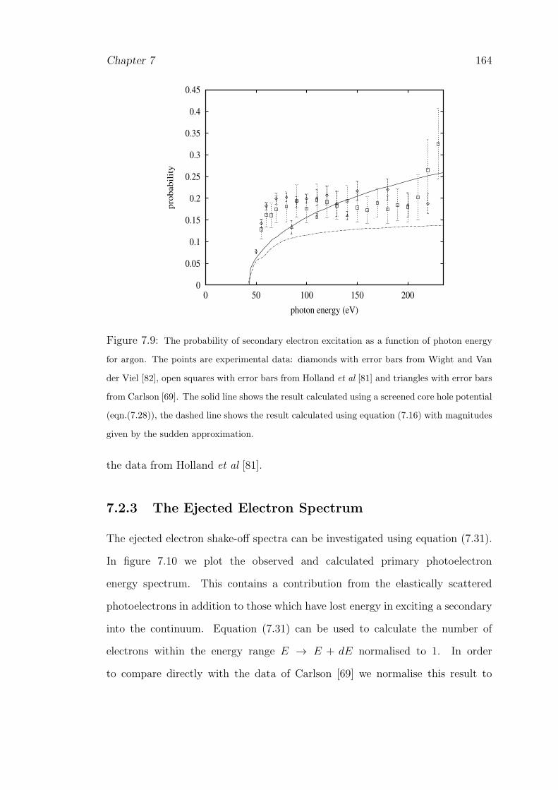
Chapter 7 164
0
0.05
0.1
0.15
0.2
0.25
0.3
0.35
0.4
0.45
0 50 100 150 200
pro
bab
ilit
y
photon energy (eV)
Figure 7.9: The probability of secondary electron excitation as a function of photon energy
for argon. The points are experimental data: diamonds with error bars from Wight and Van
der Viel [82], open squares with error bars from Holland et al [81] and triangles with error bars
from Carlson [69]. The solid line shows the result calculated using a screened core hole potential
(eqn.(7.28)), the dashed line shows the result calculated using equation (7.16) with magnitudes
given by the sudden approximation.
the data from Holland et al [81].
7.2.3 The Ejected Electron Spectrum
The ejected electron shake-off spectra can be investigated using equation (7.31).
In figure 7.10 we plot the observed and calculated primary photoelectron
energy spectrum. This contains a contribution from the elastically scattered
photoelectrons in addition to those which have lost energy in exciting a secondary
into the continuum. Equation (7.31) can be used to calculate the number of
electrons within the energy range E → E + dE normalised to 1. In order
to compare directly with the data of Carlson [69] we normalise this result to

Chapter 7 165
Carlson’s at the second peak in the shake-off spectrum due to 2p,2s shake off. We
also use an energy scale of ’Channels’, where 1 Channel = 2.05 eV and a channel
of zero corresponds to an electron energy of 100 eV, as in Carlson’s paper. To
obtain the relative sizes of the peaks for the elastically scattered photoelectrons
we have examined the ratio of the 2p and 2s contributions to the absorption
coefficient. We find µ2po /µ
2so = 1.89, this is the ratio between the number of 2p
and the number of 2s photoelectrons created. From Carlson’s data we can see
that experimentally we obtain approximately twice as many 2p photoelectrons as
2s photoelectrons. In plotting our data we have normalised the 2p peak to that
of Carlson and broadened the energy distributions using a Gaussian of half width
2.05 eV centred on the 2p and 2s binding energies.
0 10 20 30 40 50 60 70 80 90
CHANNEL
101
102
103
104
INT
EN
SIT
Y (
arb
itra
ry u
nit
s)
Figure 7.10: The primary photoelectron energy spectrum. The graph on the left is calculated
using the screened core hole potential as described in the text. The graph on the right is
reproduced from Carlson [69].
The inelastic part of the calculated secondary electron spectrum does not show
the same features as that measured experimentally. The calculated shake-off

Chapter 7 166
peaks are too broad and we do not obtain the correct ratio between 2p,2p shake-
off and 2s, 2p shake-off. From the previous section, however, we know that the
total number of electrons (the area under the curve) is about right. We also
obtain a reasonable agreement in the fall off in the number of primary electrons
with energy. The intensity falls from ∼ 100 at the 2s, 2p peak to approximately
15 at 5 channels, compared to Carlson’s measured value of about 20 at 5 channels.
We believe the discrepancies between the calculated and measured results are
due to inaccuracies in the calculated low energy, final state phase-shifts. Unlike
the previous calculation, the calculation of the secondary electron spectrum is
sensitive to changes in the details of the atomic potential. We should therefore
use some form of energy-dependent atomic potential rather than the simple Xα
Slater exchange.
7.2.4 The Two Electron Photoionisation Cross Section
The method described in this chapter may also be used to calculate the double
electron photoionisation cross section, σ+2(ω) (eqn.(7.29)). In figure 7.11 σ+2(ω)
calculated for neon is compared to the MBPT calculations of Carter and Kelly
[71] and Chang and Poe [70].
The single electron theory, using a screened core hole potential gives results
comparable to those produced using complex, many-body, multi-configuration
wavefunctions. We would claim that our method is much easier to implement
and, as it can produce a set of probabilities for the full range of energies for
a given element in under 30 seconds, is probably much quicker to use than any
comparable many-body calculation. Carter and Kelly [71] use their MBPT theory
method to give good agreement with the argon data and less good agreement with
the neon shake-off data. Their calculated results fit the experimental neon cross

Chapter 7 167
60 160 260
photon energy (eV)
0
10
20
30
σ2
+(c
m2)
Figure 7.11: The two electron excitation cross section for neon. The solid line gives the
calculated result from equation (7.29). The long dashed line is that produced by Chang and
Poe [70], whereas the short dashed line and the dotted line are calculated by Carter and Kelly
[71]. The short dashed line is calculated using the V N−1 potential and the dotted line using
the V N−2 potential. The results by Carter and Kelly [71] and Chang and Poe [70] have been
reproduced from figure 7 of reference [71].
sections well at high energies but not between ω = 60 eV to ω = 135 eV. They
claim that this is a fault of the potential used. The V N−2 potential, calculated
with 2 electrons missing from the atom, overestimates σ2+(ω), whereas the V N−1
potential (with one electron missing from the atom) underestimates the cross
sections at low energies. Carter and Kelly claim that the physical situation lies
somewhere between the two cases and could be obtained by including more terms
in the perturbation series. By screening our core hole potential we obtain results
for the cross section which bisect the two curves of Carter and Kelly at low
energies. We already know from figure 7.5 that we obtain reasonable agreement
with experiment at low energies. At high energies, however, the cross section

Chapter 7 168
calculated using equation (7.29) is larger than those produced by Carter and
Kelly or by Chang and Poe. This is probably because we underestimate the
screening of the core hole at high photoelectron energies. This overestimates the
two electron cross section and therefore gives larger than expected results for the
shake-off probabilities at high photon energies.
7.2.5 The Two Electron Absorption Coefficient
In section 7.1.3 we discussed an approximate method for determining the
two electron absorption coefficient. Strictly speaking, in the time-dependent
perturbation theory discussed, the single and double electron absorption
coefficients are identical. However, in section 7.1.3 we used an ad-hoc argument
in order to obtain an idea of the shape of the two electron X-ray absorption
coefficient.
19000
20000
21000
22000
23000
0 100 200 300 400 500 600
µ(ω
)
photon energy above the k edge (eV)0 100 200 300 400 500 600
photon energy above the K−edge (eV)
0
0.2
0.4
0.6
0.8
1
∆µ
/µκ (
%)
Figure 7.12: The two electron absorption coefficient for Bromine. The graph on the left
shows a comparison between the X-ray absorption coefficient calculated using a purely one
electron calculation (the dotted line) and µ(ω) calculated using equation (7.36) (the solid line).
The graph on the right shows the difference between the two curves normalised to the K-edge
absorption as a percentage.
On the left of figure 7.12 we show the X-ray absorption coefficient for Bromine

Chapter 7 169
as a function of photon energy. The single and double electron absorption
coefficients have very similar magnitudes. This must be the case because, first,
both calculations satisfy the sum rule, and second, single electron calculations
of µ(ω) such as those produced by Veigele [47] give reasonable agreement with
experiment. From detailed experimental studies of multiple electron excitations
by, for example Deutsch and Hart [78], Kodre et al [85] and Filipponi [86] we
know that the features produced on the absorption edge due to multiple electron
excitations are small, of the order of 1%. Although the total contribution to µ(ω)
from two electron events is approximately 20−30% the two electron excitations do
not produce sharp jumps in the absorption coefficient of this magnitude because
of the slow cut in of the multiple electron transition probabilities with energy.
Experimentally the two electron shake-off events can be seen as bumps on the
absorption coefficient [86]. We do not see these features on the calculated two
electron absorption coefficient because, in this model, the energy dependence is
too slow. From the curve to the right of figure 7.12 we can see, however, that we
do obtain multiple electron features of about the right order of magnitude. In
calculating ∆µ/µk in figure 7.12 we have assumed the one electron calculation to
be equivalent to the smooth atomic background. The difference between the one
and two electron calculations (∆µ) therefore shows up the multi-electron features.
7.2.6 The Amplitude Reduction Factor
The probability of secondary electron shake-off is very closely related to the
amplitude reduction factor used in EXAFS. This factor is used in the purely
one electron EXAFS calculation to account for many-electron excitations at the
absorbing atom. We argued previously that only those photoelectrons which did
not excite passive electrons into the continuum would contribute to the EXAFS

Chapter 7 170
signal, thus the amplitude reduction factor is simply the probability that none of
the secondary electrons are excited into the continuum,
s2o(ω) = 1− P (ω), (7.37)
where P (ω) may be taken from equation (7.15) or from equation (7.28) with the
relevant modifications as discussed in the text.
The theory used in this chapter describes both the photoelectron and the core
hole, it includes both the intrinsic and extrinsic EXAFS loss processes at the
central atom. At high energies, of course, the extrinsic losses tend to zero and
equations (7.15) and (7.28) reduce to the sudden limit for the shake-off probability
discussed in chapter 6. Because equation (7.37) for the amplitude reduction factor
includes all the EXAFS losses at the central atom we cannot use it directly in
equation (1.3) for the EXAFS. We must first modify the mean free path term in
equation (1.3) so that it describes the extrinsic losses only at the scattering atom.
For the mean free path term we therefore have, exp ( − 2(rj − ro)/λ), where rj
is the distance to the scattering atom and ro subtracts off the contribution from
the central atom.
In section 7.2.2 we obtained results, effectively for s2o(ω), that agreed well with
experimental data for neon and argon following K-edge photoabsorption. In figure
7.13 we compare values of s2o(ω) calculated using the two methods in this chapter
with data produced by Stern et al [87] for Bromine. The magnitudes of the data
and the two calculated sets of results agree well at high photon energies although
the result calculated using the screened core hole is still falling at 700 eV above
the edge. Both the calculated curves cut in far quicker than the experimentally
measured set of points. The measured amplitude reduction does not deviate from
unity until approximately 100 eV above the edge, this is therefore the primary
photoelectron energy at at which the first secondary electrons are excited into

Chapter 7 171
the continuum. We find this result surprising. The most weakly bound state in
Bromine has a binding energy of only ∼ 5 eV [29] which suggests that we should
see secondary electrons excited into the continuum at a photon energy of at most
10 eV above the K-edge. Data from Kodre et al [85] supports this view. Kodre
et al find the onset of the 3d shake-off in Bromine to be 90 eV above the K-edge.
The 4s and 4p shake-off must appear at much lower energies than this.
0.7
0.75
0.8
0.85
0.9
0.95
1
1.05
0 100 200 300 400 500 600 700
Am
pli
tud
e R
ed
ucti
on
photon energy above the K edge (eV)
Figure 7.13: The amplitude reduction factor (1 − P (ω)) as a function of the photon energy
above the K-edge for Bromine. The solid line shows the result calculated using the sudden
approximation with a model energy dependence (eqn.(7.16)) whilst the dashed line shows s2o(ω)
calculated using the screened hole potential (eqn.(7.28)). The diamonds with error bars are
experimental data measured by Stern et al [87].
In figure 7.14 we have plotted the amplitude reduction factor against photon
energy above the K-edge for copper, silicon and silver. The points give the results
calculated using a model energy dependence and the sudden approximation whilst
the lines are values of s2o(ω) calculated using the screened core hole. From chapter
6 we know that the sudden approximation gives reasonable high energy limits for

Chapter 7 172
Figure 7.14: The amplitude reduction factor (1 − P (ω)) as a function of the photon energy
above the K-edge. The solid line shows the result calculated using a screened core hole potential
(eqn.(7.28)) for copper, the dashed line for silicon and the dotted line for silver. The points are
results found using the sudden approximation and a model energy dependence: diamonds for
copper, crosses for silicon and squares for silver.
the amplitude reduction. The energy dependence also fits in with the commonly
held view that s2o(ω) reaches its full magnitude within at most a couple of hundred
volts of the edge. The results using the screened core hole for copper and silicon
are also surprisingly good. The energy dependence seems reasonable and the
magnitudes are within 15% of those given by the sudden approximation at 800
eV above the edge. The screened core hole result for silver is not so good. The
amplitude reduction varies much more slowly with energy than we would expect
and looks to be tending toward a high energy limit of less than 0.6, compared to
the sudden approximation result of 0.8. We believe that the poor results for Silver
may be due to the large number of weakly bound electrons in the 4d orbitals.
The calculation for silver is more sensitive to changes in the low energy final

Chapter 7 173
state phase-shifts. It may be that, in this case, the Slater Xα potential is an
inadequate representation of the true electronic exchange.
7.2.7 Connection with EXAFS Data Analysis
In this chapter we have described a method by which an energy-dependent
amplitude reduction factor may be quickly calculated for all edges of all elements.
This factor can then be used, along with the appropriate mean free path term, in a
single electron theory using real atomic scattering potentials to calculate EXAFS
of the correct magnitude. Of course, the losses to the photoelectron wave could
be evaluated using a complex scattering potential and, from chapter 4, we know
that the Hedin-Lundqvist (HL) potential gives a good, if somewhat fortuitous,
agreement with experiment. However data analysis programs using complex
scattering potentials are complex to write and maintain, especially when multiple
scattering must be taken into account. Programs using only real potentials are
extremely simple in comparison. The Dirac-Hara exchange potential gives better
phase-shifts for EXAFS purposes than the real part of the HL potential [53].
Using this real scattering potential and an energy-dependent loss factor such as
that described in this chapter we would expect to obtain good EXAFS spectra
without the complications of the complex phase-shift approach.
In figure 7.15 we compare calculated EXAFS spectra for copper metal. As
described in chapter 4, section 4.2.4, we used the Daresbury program EXCURV98
[14] to calculate an EXAFS spectrum for Cu foil with both the HL (solid line)
and the Xα potentials using only the first shell of scattering atoms. The spectra
calculated using the Xα exchange is slightly out of phase with the best fit HL
spectra, it is also much larger as it includes none of the losses to the photoelectron
beam from inelastic scattering.

Chapter 7 174
-0.3
-0.25
-0.2
-0.15
-0.1
-0.05
0
0.05
0.1
0.15
0.2
0 1 2 3 4 5 6 7 8
EX
AF
S
k (atomic units)
-0.3
-0.25
-0.2
-0.15
-0.1
-0.05
0
0.05
0.1
0.15
0.2
0 1 2 3 4 5 6 7 8
EX
AF
S
k (atomic units)
Figure 7.15: Unweighted EXAFS spectra for copper foil. The solid curve gives the result
calculated with the Daresbury program EXCURV98 using the Hedin-Lundqvist exchange
potential. The two sets of points are the spectra obtained using the real Xα potential in
EXCURV98 multiplied by the two types of loss factors investigated in this chapter. The curve
on the left is with a loss factor calculated using a model energy dependence and normalised
to the sudden approximation whilst the graph on the right is with a result calculated using a
screened core hole.
To obtain the curves denoted by diamonds in figure 7.15 we multiply the Xα
EXAFS spectra with the energy-dependent loss factors calculated in this chapter
and by a mean free path term, exp (−2(rj−ro)VPI/k), where rj = 2.541 A is the
nearest neighbour distance, ro = 1.27 A is the central atom muffin tin radius and
VPI = 4 eV. The curve on the left shows the spectra obtained with a loss factor
given by equation (7.16) normalised to a sudden limit of 0.67. The curve on the
right shows the spectra calculated using the screened core hole loss factor. Both
loss factors seem to give a reasonable description of the losses, both significantly
improve the fit from that obtained with the Xα potential alone and both factors
are considerably better than the constant s2o and VPI loss factors used historically.
Because the spectra are slightly out of phase it is not particularly instructive to
give an R-factor value for the comparison of the various theories. However, both
the model energy dependence curves give an R-factor of around 42%. This is
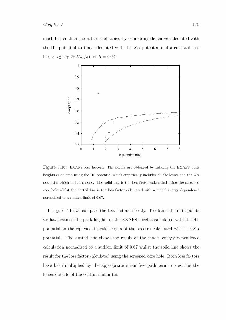
Chapter 7 175
much better than the R-factor obtained by comparing the curve calculated with
the HL potential to that calculated with the Xα potential and a constant loss
factor, s2o exp(2rjVPI/k), of R = 64%.
0.3
0.4
0.5
0.6
0.7
0.8
0.9
1
0 1 2 3 4 5 6 7 8
Am
pli
tud
e
k (atomic units)
Figure 7.16: EXAFS loss factors. The points are obtained by ratioing the EXAFS peak
heights calculated using the HL potential which empirically includes all the losses and the Xα
potential which includes none. The solid line is the loss factor calculated using the screened
core hole whilst the dotted line is the loss factor calculated with a model energy dependence
normalised to a sudden limit of 0.67.
In figure 7.16 we compare the loss factors directly. To obtain the data points
we have ratioed the peak heights of the EXAFS spectra calculated with the HL
potential to the equivalent peak heights of the spectra calculated with the Xα
potential. The dotted line shows the result of the model energy dependence
calculation normalised to a sudden limit of 0.67 whilst the solid line shows the
result for the loss factor calculated using the screened core hole. Both loss factors
have been multiplied by the appropriate mean free path term to describe the
losses outside of the central muffin tin.

Chapter 7 176
Within the range of an EXAFS spectra the model energy dependence
calculation gives excellent agreement with the losses obtained using the HL
potential, with much less computational effort. The screened core hole also gives
reasonable results although the energy dependence is not quite correct. The
energy dependence of both the loss factors is unphysical at small k because of the
constant value for VPI used in the mean free path term. This completely kills the
EXAFS at very small k. To model the mean free path term more accurately we
need an energy-dependent VPI , the simplest form being one which simply cuts
off at the binding energy of the most weakly bound state. Below this energy, no
inelastic scattering is possible and thus we obtain no losses to the EXAFS.
7.3 Conclusion
In this chapter we have used time-dependent perturbation theory and a model
core hole - photoelectron potential, V (r), to obtain results for the secondary
electron shake-off probabilities as a function of photon energy above the X-ray
absorption edge.
Initially we follow the procedure of Thomas [21]. We model the energy
dependence of the radial matrix element involving V (r) and set its magnitude
using the high energy limit for the shake-off probabilities which may be calculated
using the sudden approximation (see chapter 6) or taken from experiment. We
extend Thomas’ model to correctly obtain the probabilities for secondary electron
shake-off rather than shake-up by including the possibility of transitions into all
energetically available continuum states. This method gives results for the shake-
off probabilities which compare very well with experimental data for neon and
argon. This method can also be used to generate an energy-dependent loss factor
applicable to EXAFS calculations which use a real scattering potential. The

Chapter 7 177
results obtained using the Xα potential and the energy-dependent loss factor
agree extremely well with those obtained using the complex HL potential which
is known to give good agreement to experiment.
In a further extension to Thomas’ theory we model V(r) explicitly. We choose a
form for the potential which starts at zero at small times and tends to a screened 1r
potential once the primary photoelectron has departed from the atom. We found
that the results obtained were fairly dependent on the form of screening used.
However, an SPP dielectric function used within the local density approximation
gave results which agree reasonably well with experiment. The energy dependence
of the shake-off probabilities is, however, not quite correct. The dielectric function
used appears to underestimate the screening at high photoelectron energies,
although the magnitudes obtained are generally within the experimental error
over the region of energy of interest in EXAFS. This method gives double
electron absorption cross sections which are as good as those produced using the
configuration interaction method. However, the secondary electron excitation
spectra produced using the screened core hole are, at best, acceptable, the energy
dependence of the spectra being incorrect. This method does, however, show
promise, and it may be that calculations with a better form for the dielectric
function or more accurate final state wavefunctions would greatly improve the
results. Again, using this method to generate an energy dependent loss factor for
EXAFS calculations would appear to give results as good as those obtained with
HL potential.
In summary we have investigated two methods which give reasonable results
for the energy dependence and magnitude of the secondary electron shake-off
probabilities. Both methods can be used to generate energy-dependent loss
factors which may be used in real potential EXAFS scattering codes to give
good agreement with the experimental EXAFS.

Chapter 8
Summary and Conclusions
In this thesis we have investigated some of the many-electron effects which
affect the X-ray absorption fine structure or EXAFS. EXAFS is an important
experimental technique of particular use for the study of the structure of non-
crystalline materials. Data analysis of the EXAFS is generally performed by
comparing the experimental spectra to spectra calculated theoretically using
plausible model structures. To date the theory has been developed using a
wholly single electron formalism with the many-body effects, which are not well
understood, typically lumped into various empirical parameters and scattering
potentials. These many-electron effects are, however, important. In particular
they have a large effect on the EXAFS amplitude which greatly affects the
experimental determination of coordination numbers. Typically, the EXAFS
technique cannot determine coordination numbers to an accuracy of better than
±10%.
In this thesis we investigate some of the approximations used to describe many-
electron effects in EXAFS data analysis programs. The Daresbury program
EXCURV98 [14] uses a complex exchange and correlation potential to model the
many-electron effects. The imaginary part of this potential models the extrinsic
178

Chapter 8 179
inelastic losses to the EXAFS. It therefore reduces the EXAFS amplitude. In
chapter 2 we develop approximations which allow us to calculate the amplitude of
the EXAFS in the presence of a complex scattering potential without calculating
the EXAFS itself. This allows us to study the effect of the imaginary potential
on the theoretical amplitudes without having to consider the other changes to
the EXAFS spectra caused by the complex potential.
The exchange and correlation potential most commonly used today is the
Hedin-Lundqvist [9] potential which is derived from the GW formalism using
uniform electron gas relations and the local density approximation. This potential
lumps all of the inelastic scatterings into collective excitations, the plasmons,
without explicitly mentioning the single electron transitions. The HL potential
neglects single electron excitations because it is calculated using an approximate
form of the inverse dielectric function, the single plasmon pole form [9]. In
chapter 3 we examine the SPP dielectric function and compare it to a full atomic
calculation of ǫ−1(q, ω). To our knowledge this is the first such calculation of
an atomic ǫ−1. The two forms show similar overall energy and q dependence.
The SPP dielectric function, however, does not exhibit the sharp structure of the
atomic calculation at the X-ray absorption edges because of its neglect of the
single electron excitations.
In chapter 4 we use the SPP dielectric function to calculate the HL potential.
The effects of the imaginary part of this potential on the EXAFS amplitudes
are then examined using the formulae derived in chapter 2. We find that the
HL potential significantly overestimates the extrinsic EXAFS losses. It gives
values for the mean free path which are much shorter than those observed
experimentally. Instead the amplitudes given by the HL potential agree well
with the total (extrinsic plus intrinsic) losses to the EXAFS. Additional amplitude
fitting parameters should therefore not be used when data fitting with the HL

Chapter 8 180
potential. This is an important result. Previously it had been assumed that the
HL potential gave a good approximation to the extrinsic losses, thus, values of the
amplitude reduction factor of 0.6 to 0.8 were considered reasonable when data
analysing using this potential. Using such low values, however, would lead to
erroneous results for the Debye-Waller factor and for the coordination numbers.
This has now mostly been acknowledged amongst the UK EXAFS community,
the default value of the constant amplitude fitting parameter, AFAC (s2o), in
EXCURV has been changed from 0.8 in the 1992 release to 1.0 in the current
version.
In chapter 5 we develop the work of Beni, Lee and Platzman [18] who
produced a complex scattering potential which explicitly includes single electron
excitations. BLP derive their potential from a consideration of the atomic
scattering factor. In chapter 5 we show that this potential may also be obtained
from the GW approximation by making the relevant approximations. We derive
a method by which we may solve for the BLP potential without using the many
approximations applied by BLP. However, we find that the imaginary part of the
potential is much larger than the imaginary part of the HL potential and therefore
vastly overestimates the inelastic scatterings. We find that the magnitude of
the potential is critically dependent on the phase-shifts and hence the potential
itself. A proper calculation of the BLP potential would require a self-consistent
procedure taking many iterations. However, such a procedure is not practical for
EXAFS data analysis purposes where computer time must be kept to a minimum.
We therefore conclude that this potential is unsuitable for EXAFS purposes.
In chapter 6 we change tack somewhat and examine the intrinsic losses to
the EXAFS. In this chapter we discuss the problem in terms of the sudden
approximation which is valid in the limit of high photoelectron energy. By
describing the appearance of the core hole using Slater’s rules [20] we may easily

Chapter 8 181
calculate the effects on the EXAFS amplitudes in this limit for all edges of
all elements, the first time that this has been done. We find that, using this
simple model with numerical values for the effective nuclear charge tabulated
by Clementi et al [27], we obtain surprisingly good agreement with experiment.
The method can also be used to calculate the probability of excitation into the
continuum and the probability of transitions into excited bound states which
we find to be small. In this chapter we also calculate the amplitude reduction
factor using tight binding initial state wavefunctions. In the worst possible case
this calculation gives results which differ at most by ±10% from the free atom
calculation of s2o. We therefore conclude that the amplitude reduction factor is
independent of the chemical environment of the absorbing atom.
Chapter 7 is concerned with a time-dependent model of the core hole -
photoelectron system. We take a simple model form for the time dependence
of the potential of the core hole and photoelectron and use it to calculate results
for the secondary electron shake-off probabilities. The time-dependent form of
the potential comes from Thomas [21] who calculated the neon shake-off spectra
by normalising his results to the experimental high energy limit. Thomas’ theory
is, however, incorrect. We correct the theory of Thomas and calculate shake-off
spectra for neon, and argon K and L edges either by normalising to experiment
or to the calculated results of chapter 6. The calculations are compared to
experiment and are found to agree well. We also describe a more complex model of
the core hole - photoelectron system in which we explicitly include the screening
of the core hole by using the SPP dielectric function. This calculation gives
less good results than the simpler model used but is at least as good as the
many-body perturbation theory models which have been used previously [70, 71].
The results obtained for the shake-off spectra can be used to calculate the total
(intrinsic+extrinsic) losses to the EXAFS. The total EXAFS losses appear to

Chapter 8 182
agree well with experiment thus, this method could be used with an entirely real
scattering potential in an EXAFS data analysis program. Chou et al [53] state
that the Dirac-Hara potential (a real scattering potential) gives better final state
phase-shifts than the HL potential. Also, data analysis programs with complex
potentials are difficult to produce, especially where multiple scattering must be
taken into account. Using the methods described in this chapter it would be
relatively simple to produce an EXAFS data analysis program using the Dirac-
Hara potential but which also adequately describes the inelastic losses. In such
a program the energy dependent loss factors calculated in this Chapter could be
input for each element in parameterised form. In most data analysis programs
the intrinsic losses are approximated by a constant or are included in an ad hoc
manner by the use of the HL potential. The method described in chapter 7,
however, does not suffer from this drawback, and would also be of use to groups
who do not readily have access to such codes as EXCURV98.
A possible future work stemming from this thesis would, of course, be to
produce such a multiple scattering EXAFS program using the methods described
above. This program could then be tested fully against the presently available
codes. Also, other interesting results have been produced in this thesis. Namely,
whilst being good enough at present, the approximations made to describe many-
body effects in EXAFS are not accurate. Restrictions, largely due to the lack of
available computing power mean that we cannot do much better than the HL or
other similar potentials. However, improvements could be made to the results
reported in this thesis by using fully self-consistent calculations and including
higher order terms in the perturbation theories. A further study along these lines
might produce results of interest for their own sake.

Appendix A
The Real Part Of The
Hedin-Lundqvist Potential
In Chapter 4, equation (4.12), the real part of the Hedin-Lundqvist potential was
defined in terms of 3 coefficients. I1, I2 and I3 are the results of the angular
integrals in equation (4.10). These are listed below.
I1 =Ef −Ei
klog
∣
∣
∣
∣
∣
k + kfk − kf
∣
∣
∣
∣
∣
+ kf (A.1)
I2 =1
kq2clog
∣
∣
∣
∣
1− qck
∣
∣
∣
∣
− 1
k3log
∣
∣
∣
∣
∣
1 +k
qc
∣
∣
∣
∣
∣
+1
k2qc(A.2)
I3 =1
k2
{
1
qmin− 1
qc− 1
qmax
}
+1
kq2maxlog
∣
∣
∣
∣
1− qmaxk
∣
∣
∣
∣
+1
kq2clog
∣
∣
∣
∣
1− qck
∣
∣
∣
∣
+1
k3log
∣
∣
∣
∣
∣
qc(qmin − k)qmaxqmin(qc − k)(qmax − k)
∣
∣
∣
∣
∣
− 1
kq2minlog
∣
∣
∣
∣
∣
(k − qmin)(q2min − 2Ef + 2Ei)
k(q2min + 2Ef − 2Ei
∣
∣
∣
∣
∣
+1
2Ef − 2Eilog
∣
∣
∣
∣
∣
q4min(q2max − 2Ef + 2Ei)(q
2max + 2Ef − 2Ei)
q4max(q2min − 2Ef + 2Ei)(q
2min + 2Ef − 2Ei)
∣
∣
∣
∣
∣
− 1
kq2maxlog
∣
∣
∣
∣
∣
q2max − 2Ef + 2Eiq2max + 2Ef − 2Ei
∣
∣
∣
∣
∣
qc < qmin
=1
k2qmax− 1
k3log
∣
∣
∣
∣
∣
1 +1
qmax
∣
∣
∣
∣
∣
+1
kq2clog
∣
∣
∣
∣
∣
q2c − 2Ef + 2Eiq2c + 2Ef − 2Ei
∣
∣
∣
∣
∣
183

Appendix A 184
+1
2Ef − 2Ei
{
log
∣
∣
∣
∣
∣
q2max − 2Ef − 2Eiq2min − 2Ef − 2Ei
∣
∣
∣
∣
∣
+ log
∣
∣
∣
∣
∣
q2max + 2Ef − 2Eiq2c + 2Ef − 2Ei
∣
∣
∣
∣
∣
}
+2
Ef −Eilog
∣
∣
∣
∣
∣
qcqmax
∣
∣
∣
∣
∣
qmin < qc < qmax
=1
kq2clog
∣
∣
∣
∣
1− qck− 1
k3
∣
∣
∣
∣
log
∣
∣
∣
∣
∣
1− k
qc
∣
∣
∣
∣
∣
− 1
k2qcqc > qmax (A.3)

Appendix B
Derivation of the Beni, Lee and
Platzman Polarisation Potential
from the Atomic Scattering
Factor
In Chapter 5 we briefly discussed how Beni, Lee and Platzman (BLP) obtained
their form for the complex correlation potential. In this appendix we outline the
method in more detail.
BLP [18] define their form for the potential as the Fourier transform of the
atomic scattering factor, f(η). The scattering factor, summed to all orders of
scattering, may be written in terms of the exact many body wavefunctions of the
system and the interaction potential seen by the photoelectron,
f = − 1
2π〈ΨI |Vint |ΨF 〉, (B.1)
where ΨI is a many body state with the photoelectron far from the atom and the
atomic electrons unperturbed, and ΨF is the many body final state describing the
185

Appendix B 186
atomic electrons and the scattered photoelectron far from the atom. As we are
interested only in the elastic scattering, ΨF must have all of the bound electrons
in their initial atomic states.
Vint, the potential seen by the photoelectron, is given by,
Vint = −Zr+∑
i
1
|r− ri |, (B.2)
where Z is the atomic number and the summation is over all electronic
coordinates.
Equation (B.1) may also be expressed in the first Born approximation in terms
of an effective scattering potential,
f(η) = − 1
2π〈ϕki
|Veff |ϕkf〉. (B.3)
Equation (B.3) describes the scattering by an atom of some incident electron
from wavevector ki to kf where the momentum transfer, kf − ki, is given by η
and ϕkiand ϕkf
are plane waves.
To obtain the BLP result we must neglect the exchange between electrons in
equation (B.1) so that ΨI and ΨF become Hartree products of the photoelectron
and bound state wavefunctions. We take the photoelectron initial state to be
a plane wave and obtain the many electron final state using a Green function
expansion.
ΨF = ΨK +GVintΨK . (B.4)
ΨK is the product of all the bound atomic states and a plane wave final state of
wavevector, kf , and the Greens function is defined as,
G =∑
N
ΨNΨ∗N
E − EN ± ıδ, (B.5)
where ΨN are the Hartree wavefunctions for all of the excited states available to
the system. Within the Hartree approximation only those states with at most

Appendix B 187
a single excited electron are obtainable. EN is the energy of the many electron
state, ΨN , and E = EI +12k2i is the sum of the initial photoelectron energy and
the energies of all the bound state electrons in the system.
Substituting for ΨF into equation (B.1) we have that,
f(η) = − 1
2π
{
〈ΨI |Vint |ΨK〉+∑
N
〈ΨI |Vint |ΨN〉〈ΨN |Vint |ΨK〉E − EN ± ıδ
}
= f1 + f2. (B.6)
As ΨI is simply a product of bound atomic orbitals, φo(ri), and a free electron
wave, we can see that the first term in equation (B.6) is simply the Fourier
transform of the Hartree potential,
f1(η) = − 1
2π
∫
e−ıη·r(
−Zr+∑
i
∫
φ∗o(ri)φo(ri)
|r− ri |dri
)
dr. (B.7)
The second term in equation (B.6) must therefore be the Fourier transform of
the correction to the Hartree potential. This correction term is the polarisation
potential.
In evaluating f2 we write the excited, intermediate, state wavefunction as,
ΨN = eı(ki+q)·r∏
j 6=iφj(rj)ψn(ri). (B.8)
Within the Hartree approximation, we may choose a particular electron to be
excited from a bound atomic orbital, φo(ri), into an excited continuum state,
ψn(ri). The photoelectron is excited into the intermediate state, exp(ı(ki+q) ·r),
thus the energy of the many electron wavefunction, ΨN , is given by,
EN = EI − ωo + ωn +1
2|ki + q |2, (B.9)
where ωo and ωn are the energies of the single electron bound and excited states.
The integrals over the photoelectron radial coordinate are simply Fourier
transforms of the 1/r potentials. These may be easily evaluated. Then, to obtain

Appendix B 188
the BLP result for the scattering factor we must finally integrate over all the
possible intermediate photoelectron states available for each of the ψn(r) excited
atomic states.
f2(η) = − 1
(2π)3∑
n
∫
dq8π〈φo |eıq·r |ψn〉〈ψn |eı(η−q)·r |φo〉q2 |η − q |2 (E − EN + ıδ)
=1
2π2
∑
n
∫
dq〈φo |eıq·r |ψn〉〈ψn |eı(η−q)·r |φo〉
q2 |η − q |2 (q2 + 2q · ki + 2(ωn − ωo)− ıδ),(B.10)
where we have taken the +ıδ term in the denominator of the Green function as
the excited states ψn(r) must be unoccupied.
Equation (B.10) is identical to the result for the second Born approximation
to the atomic scattering factor given by BLP. f2 is just the Fourier transform of
an effective scattering potential which may be added to the Hartree potential to
give an approximation to the electron-electron correlation.

Appendix C
Calculation of an using a
Different q Dependent Plasmon
Frequency.
In chapter 7 we calculated the probability, P (ω), of exciting two electrons into
the continuum following the absorption of an X-ray photon. The results obtained
were strongly dependent on the form of the screening used. In Chapter 7 we
calculated P(ω) using a single plasmon pole dielectric function (eqn.(7.20)) with
a simplified q dependent plasmon frequency of, ω2q = ω2
p(r) +14q4. We can also
calculate the relevant excitation probabilities using a less accurate form of the q
dependent excitation frequency,
ωq = ωp(r) +1
2q2. (C.1)
This form of the plasmon frequency has identical large and small q limits to the
q4 plasmon frequency defined above.
The probability of secondary electron excitation is defined in terms of the
189

Appendix C 190
expansion coefficients of the perturbed system wavefunctions. We have,
an =ı
(2π3)
⟨
ψn
∣
∣
∣
∣
∫
dqeıq·rV (q,−ωno)ǫ−1(q,−ωno)∣
∣
∣
∣
φlo
⟩
(C.2)
Using equation (C.1) for the q dependent plasmon frequency we can, once again,
evaluate the q integral in equation (C.2) directly with the help of Gradsteyn and
Ryzhik [56]. We find,
an =ıt−1o
ωno(ωno + ıt−1o )
⟨
ψn
∣
∣
∣
∣
∣
1
r+
ω2p
rωno
[
1
a2(1− cos(ar)) +
1
b2
(
1− e−br)
]
∣
∣
∣
∣
∣
φo
⟩
ωno > ωp(r)
=ıt−1o
ωno(ωno + ıt−1o )
⟨
ψn
∣
∣
∣
∣
∣
1
r+
ω2p
rωno
[
1
a2
(
1− e−ar)
+1
b2
(
1− e−br)
]
∣
∣
∣
∣
∣
φo
⟩
ωno < ωp(r) (C.3)
where,
a2 = 2|ωno − ωp| and,
b2 = 2(ωno + ωp). (C.4)
The r integrand contains a divergence at ωno = ωp(r). This may be dealt using a
Romberg integration routine in the same way as the r integral in Chapter 7.

Bibliography
[1] R de L. Kronig, Z. Phys. 70 (1931) 317-323.
[2] D E Sayers, E A Stern and F W Lytle, Phys. Rev. Lett. 27 (1971) 1204-1207.
[3] E A Stern, Phys. Rev. B 10 (1974), 3027-3037.
[4] P A Lee and J B Pendry, Phys. Rev. B 11 (1975) 2785-2811.
[5] J J Rehr, R C Albers, submitted to, Reviews of Modern Physics.
[6] S J Gurman and R F Pettifer, Philos. Mag. B 40 (1979) 345-349.
[7] H A Bethe, R Jackiw, ’Intermediate Quantum Mechanics’, (The
Benjamin/Cummings Publishing Company (1986)).
[8] J B Pendry, ’Low Energy Electron Diffraction’, (Academic Press, London
(1974)).
[9] L Hedin and S Lundqvist, Solid State Physics, 23 (1969) 2-181.
[10] P A Lee and G Beni, Phys. Rev. B 15 (1976) 2862-2883.
[11] T A Carlson, C W Nestor, T C Tucker and F B Malik Phys. Rev. 169 (1968)
27-36.
[12] S S Hasnain (ed) ’Synchrotron Radiation and Biophysics’ (Ellis Horwood,
Chichester (1990)).
191

References 192
[13] T M Hayes and J B Boyce, Solid State Physics, 37 (1982) 173-351.
[14] N Binsted, EXCURV98: CCLRC Daresbury Laboratory computer program
(1998).
[15] W Bardyszewski and L Hedin, Physica Scripta 32 (1985) 439-450.
[16] J F Hart, Ph.D. Thesis, Leicester University (1997).
[17] M Roy, Ph.D. Thesis, Leicester University (1999).
[18] G Beni, P A Lee, and P M Platzman, Phys. Rev. B, 13 (1976) 5170-5178.
[19] L J Schiff, ’Quantum Mechanics’ 3rd edn. (McGraw-Hill, London (1968)).
[20] J C Slater, Phys. Rev 36 (1930) 57-64.
[21] T D Thomas, Phys. Rev. Letters, 52 (1984) 417-420.
[22] C A Ashley and S Doniach, Phys. Rev. B 11 (1975) 1279-1288.
[23] S J Gurman, N Binsted, and I Ross, J. Phys. C 17 (1984) 143-151.
[24] S J Gurman, N Binsted and I Ross, J. Phys. C 19 (1986) 1845-1861.
[25] T L Loucks, ’Augmented Plane Wave Method’, (W.A Benjamin inc., New
York (1967)).
[26] T A Tyson, Ph.D. Thesis, Stanford University (1991).
[27] E Clementi and C Roetti, Atomic Data and Nuclear Data Tables 14 (1974)
177-478.
[28] A D McLean and R S McLean, Atomic Data and Nuclear Data Tables 26
(1981) 197-381.

References 193
[29] ’Handbook of Chemistry and Physics’, (The Chemical Rubber Company,
Cleveland (1970)).
[30] D M Brink and G R Satchler, ’Angular Momentum’, (Clarendon Press :
Oxford (1968)).
[31] A Messiah, ’Quantum Mechanics’, vol. 1, (North Holland Publishing
Company, Amsterdam (1961)).
[32] M Abramowitz and I A Stegun, ’Handbook of Mathematical Functions’,
(Dover Publications, inc., New York (1965)).
[33] S J Gurman, J. Phys. C:Solid State Phys., 16 (1983), 2987-3000.
[34] M Roy and S J Gurman, J. Synchrotron Rad. 6 (1999) 228-230.
[35] M Roy and S J Gurman, J. Phys. IV France Colloque C2 151-152
[36] A Szabo and N S Ostlund, ’Modern Quantum Chemistry: Introduction To
Advanced Electronic Structure Theory’, (MacMillan Publishing Co., inc.
New York (1982)).
[37] F Aryasetiawan and O Gunnarson, Rep. Prog. Phys 61 (1998) 237-312.
[38] J C Slater and K H Johnson, Phys. Rev. B 5 (1972) 844-853.
[39] L Hedin, Phys. Rev. A 139 (1965) 796-823.
[40] J C Inkson, ’Many-Body Theory Of Solids. An Introduction’ , (Plenum Press.
New York and London. (1984)).
[41] W Jones and N H March, ’Theoretical Solid State Physics’ , Volume 1,
(Dover Publications, Inc. New York (1973)).

References 194
[42] D Pines, ’Elementary Excitations in Solids’, (W A Benjamin, inc. New York
(1964)).
[43] J M Ziman, ’Elements of Advanced Quantum Theory’, (Cambridge
University Press (1969)).
[44] P Nozieres, ’Theory of Interacting Fermi Systems’, (W A Benjamin, inc.
New York (1964)).
[45] J Lindhard kgl. Danske Videnskab, Selskab. Mat-fys, medd., 28 (1954) 8.
[46] K Schwarz, Phys. Rev. B 5 (1972) 2466-2468.
[47] W M J Veigele, Atomic Data Tables 5 (1973) 51-111.
[48] A Owens, S C Bayliss, P J Durham, S J Gurman, and G W Fraser,
Astrophysical Journal 468 (1996) 451-454.
[49] J Mustre de Leon, J J Rehr, S I Zabinsky and R C Albers, Phys. Rev. B 44
(1991) 4146-4156.
[50] P A M Dirac, Proc. Cambridge Philos. Soc. 26 (1930) 376-385.
[51] S Hara, J. Phys. Soc. Japan 26 (1967) 376.
[52] M S Woolfson, S J Gurman and B W Holland, Surface Science 117 (1982)
450-458.
[53] S H Chou, J J Rehr, E A Stern and E R Davidson, Phys. Rev. B 35 (1987)
2604-2614.
[54] S J Gurman, private communication.
[55] D R Penn, Phys. Rev. B 35 (1987) 482-486.

References 195
[56] I S Gradsteyn and I M Ryzhik, ’Tables of Integrals, Series and Products’,
(Academic Press, New York and London (1965)).
[57] W Magnus F Oberhettinger and R P Soni, ’Formulas and Theorems for
the Special Functions of Mathematical Physics’, (Springer-Verlag Berlin,
Heidelberg, New York (1966)).
[58] W A Harrison, ’Solid State Theory’, (Tata McGraw-Hill Publishing
Company (1970)).
[59] T Aberg, Phys. Rev. 156 (1967) 35-41.
[60] T A Carlson and M O Krause, Phys. Rev. 149 (1965) A1057-A1064.
[61] K G Dyall, J. Phys. B 16 (1983) 3137-3147.
[62] B K Teo ’EXAFS: Basic Principles and Data Analysis’, (Springer-Verlag
Berlin Heidelberg New York Tokyo (1986)).
[63] J J Rehr, E A Stern, R L Martin, E A Davidson, Phys. Rev. B 17 (1978)
560-565.
[64] G van Dorssen, private communication.
[65] J S Blakemore, ’Solid State Physics’, (Cambridge University Press (1985)).
[66] N W Ashcroft and N D Mermin, ’Solid State Physics’, (Saunders College
(1966)).
[67] K Zhang, E A Stern, J J Rehr and F Ellis, Phys. Rev. B 44 (1991) 2030-2039.
[68] S J Schaphorst, A F Kodre, J R Rusheinski, B Crasemann, T Aberg, J
T Tulkki, M H Chen, Y Azuma, and G S Brown, Phys. Rev A 47 (1993)
1953-1966.

References 196
[69] T A Carlson, Phys. Rev. 156 (1967) 142-149.
[70] T N Chang and R T Poe, Phys. Rev. A 12 (1975) 1432-1439.
[71] S L Carter and H P Kelly, Phys. Rev. A 16 (1977) 1525-1534.
[72] J W Gadzuk and M Sunjic, Phys. Rev. B 12 (1972) 524-530.
[73] E Vatai, Phys. Rev. A 38 (1988) 3777-3780.
[74] C Noguera and D Spanjaard, J. Phys. F 11 (1981) 1133-1149.
[75] D Lu and J J Rehr, Phys. Rev. B 37 (1988) 6126-6133.
[76] J Stohr, R Jaeger, and J J Rehr, Phys. Rev. Letters 51 (1983) 821-824.
[77] W H Press, B P Flannery, S A Teukolsky and W T Vetterling, ’Numerical
Recipes, The Art of Scientific Computing’, (Cambridge University Press
(1989)).
[78] M Deutsch and M Hart, Phys. Rev. Letts. 57 (1986) 1566-1569.
[79] R J Bartlett, P J Walsh, Z X He, Y Chung, E M Lee and J A R Samson,
Phys. Rev. A 46 (1992) 5574-5579.
[80] J A R Samson, R J Bartlett, and Z X He, Phys. Rev. A 46 (1992) 7277-7280.
[81] D M P Holland, K Codling, J B West and G V Marr, J. Phys. B 12 (1979)
2465-2484.
[82] G R Wight and M J Van der Viel, J. Phys. B 9 (1976) 1319-1327.
[83] U Becker, R Wehlitz, O Hemmers, B Langer and A Menzel, Phys. Rev.
Letters 63 (1989) 1054-1057.

References 197
[84] G B Armen, T Aberg, Kh R Karim, J C Levin, B Crasemann, G S Brown,
M H Chen and G E Ice, Phys. Rev. Letters 54 (1985) 182-185.
[85] A Kodre, J P Gomilsek, I Arcon, and R Preseren, J. Synchrotron Rad. 6
(1999) 306-307.
[86] A Filipponi, Physica B 208 & 209, (1995) 29-32.
[87] E A Stern, S M Heald and B Bunker, Phys. Rev. Letts. 42 (1979) 1372-1375.
[88] B H Bransden and C J Joachain, ’Physics of Atoms and Molecules’, Longman
Scientific and Technical, (1983), 494