map-based surface and subsurface flow simulation models: an
TRANSCRIPT

CRWR Online Report 96-5
Map-based surface and subsurface flow simulation models:An object-oriented and GIS approach
by
Zichuan YE, B.S., M.S., MPA., M.S.
David R. Maidment, PhD.
And
Daene C. McKinney, PhD.
August 1996
CENTER FOR RESEARCH IN WATER RESOURCES
Bureau of Engineering Research • The University of Texas at AustinJ.J. Pickle Research Campus • Austin, TX 78712-4497
This document is available online via World Wide Web athttp://www.ce.utexas.edu/centers/crwr/reports/online.html

Acknowledgments
I wish to thank Dr. David R. Maidment and Dr. Daene C. McKinney of the
Environmental and Water Resources Engineering group of the Department of
Civil Engineering, and Dr. David J. Eaton of the LBJ School of Public Affairs for
their efforts in allocating funds to financially support me through the graduate
school in the University of Texas at Austin. I would like to thank Dr. Maidment
and Dr. McKinney for supervising and guiding me through this dissertation
research. I would like, also to thank Dr. McKinney, Dr. Maidment, Dr. Edward
R. Holley, Dr. Howard M. Liljestrand, and Dr. Eaton for spending time to serve in
my dissertation committee and Dr. Holley, Dr. McKinney, Dr. Robert Herman,
and Dr. Eaton for administering my qualifying exam in 1993. Finally, I would
like to express my gratitude to my classmates and friends: Seann Reed, Francisco
Olivera, Pawel Mizgalewicz, David Watkins, Phil DeBlanc, Minder Lin, Cai
Ximin, Jessie Li, Ferdinand Hellweger, Jennifer Benaman, and Bill Saunders for
their numerous help and encouragement during my dissertation research.
Zichuan Ye
October, 1996

iii
ABSTRACT
MAP-BASED SURFACE AND SUBSURFACE
FLOW SIMULATION MODELS:
AN OBJECT-ORIENTED AND GIS APPROACH
Zichuan Ye, Ph.D.
The University of Texas at Austin, 1996
Supervisors: Daene C. McKinney, David R. Maidment
A hydrology simulation model is composed of three elements, which are
(1) equations that govern the hydrologic processes, (2) maps that define the study
area and (3) database tables that numerically describe the study area and model
parameters. When a model is constructed with its three elements separated, its
portability and user-friendliness are usually limited because any modification of
one component will not be reflected in the others. The purpose of this research is
to develop a map-based flow simulation model with all three model-components
integrated. The model is constructed under a geographic information system
(GIS) and based on the concepts of object-oriented programming. As its name
suggests, a map-based model is map-centric and it allows all the regular model
procedures such as construction, simulations, modifications, and result-processing
to be activated directly from the model maps. Based on this ‘map-centric’ and
object-oriented concept, a map-based surface/subsurface water flow simulation
model is developed and successfully applied to simulate surface and subsurface
flow on the Niger River Basin in West Africa. In the process of constructing this
map-based model, techniques are also developed to address and solve some GIS

iv
related problems such as treatment of spatially-referenced time-series data,
feature-oriented map operations, dynamic segmentation of an arc, and integration
of flows along a line.

v
Table of Contents
TABLE OF CONTENTS.............................................................................................. v
LIST OF FIGURES.................................................................................................... ix
LIST OF TABLES ....................................................................................................xii
CHAPTER ONE. INTRODUCTION ............................................................................ 1
CHAPTER TWO. SIMULATING SURFACE AND SUBSURFACE WATER FLOWS ....... 8
2.1. Concept of Object-Oriented Programming.................................................. 8
2.2. Conceptual Design of an Integrated Hydrologic Model............................. 12
2.3. Relationships between Maps, Databases and Programs ............................ 15
2.4. Governing Equations for Surface and Subsurface Water Flows................ 17
2.4.1. Equations Related to the Surface Water Flow Simulation .................. 17
2.4.1.1. The Soil -Water Balance Model.................................................... 19
2.4.1.2. Converting Time-Series between Different Spatial Features........ 23
2.4.1.3. Convolution Procedure Used To Compute Local Runoff ............. 25
2.4.1.4. Flow Routing on a River Section .................................................. 29
2.4.2. Equations Used for Groundwater Flow Simulation............................. 33
2.5. Chapter Summary....................................................................................... 40
CHAPTER THREE. A MAP-BASED SURFACE WATER FLOW SIMULATION
MODEL ............................................................................................................... 42
3.1. Introduction................................................................................................ 42
3.2. Model Construction Procedure .................................................................. 44
3.2.1. Preparing Maps for a Map-Based Simulation Model .......................... 45
3.2.2. Basic Assumptions for a Map-Based Simulation Model..................... 46
3.2.3. Construction of Basic Maps................................................................. 48
3.3. Database Design for Spatially-Referenced Time-Series Data ................... 57

vi
3.3.1. Two Types of Spatially-Referenced Data............................................ 58
3.3.2. Data Structure for Data of One-to-One Type ...................................... 58
3.3.3. Data Structure for Data of the One-to-Many Type.............................. 59
3.3.4. Connections between Databases and the GIS FTABs......................... 62
3.4. Construction of the Surface Flow Simulation Program............................. 63
3.4.1. Simulating Water Movement between River Sections........................ 64
3.4.2. Simulating Water Movement within a River Section.......................... 74
3.4.3. Simulating Water Movement within a Subwatershed ......................... 80
3.5. Other Simulation Model Objects ............................................................... 83
3.5.1. The Dam Objects ................................................................................. 83
3.5.2. The Flow-Check Point Objects............................................................ 88
3.5.3. The Flow-Diversion Point Objects ...................................................... 89
3.6. Utility Programs and Post-Processors........................................................ 89
3.6.1. Construction of a Sub-Model .............................................................. 90
3.6.2. Optimization Algorithms..................................................................... 91
3.6.2.1. The Interactive Optimization Algorithm....................................... 92
3.6.2.2. Optimization Module Based on a Direction Set Method .............. 99
3.6.3. Simulation Model Calibration ........................................................... 102
3.6.4. Flow Interpolation Module................................................................ 110
3.6.5. Plotting a Longitudinal Flow Profile ................................................. 112
3.6.6. Plotting Time-Series Data at a Selected Location ............................. 114
3.7. Chapter Summary..................................................................................... 116
CHAPTER FOUR. A MAP-BASED GROUNDWATER SIMULATION MODEL ........ 120
4.1. Introduction.............................................................................................. 120
4.2. The Construction of Model Base Maps ................................................... 121
4.3. The Simulation Model Formulation......................................................... 124

vii
4.3.1. The Construction of the Line-Loop ................................................... 126
4.3.2. The Construction of the Polygon-Loop ............................................. 129
4.3.3. Treatment of Time-Series Data Sets.................................................. 130
4.4. Treatment of Modeling Conditions.......................................................... 131
4.4.1. Treatment of Boundary and Initial Conditions.................................. 131
4.4.2. Treatment of Internal Boundary Conditions...................................... 132
4.5. The Map-Based Post-Processors and Utilities ......................................... 134
4.5.1. Plotting the Water Levels and Flow Distributions ............................ 134
4.5.2. Plotting Time Series Data at a Specified Location............................ 134
4.5.3. Modification of Model Conditions .................................................... 136
4.6. Model Verification................................................................................... 137
4.7. Chapter Summary..................................................................................... 142
CHAPTER FIVE. INTEGRATING SURFACE AND SUBSURFACE FLOW SIMULATION
MODELS ........................................................................................................... 144
5.1. Introduction.............................................................................................. 144
5.2. Construction of Surface and Subsurface Simulation Objects .................. 145
5.3. Connections between Surface and Groundwater Models ........................ 150
5.4. Simulating Through the Space and Time................................................. 152
5.5. Integration of Surface & Subsurface Water Flow Simulation Models .... 154
5.6. An Application Example of the Integrated Model................................... 156
5.7. Model Integration - Confined vs. Phreatic Aquifers................................ 163
5.8. Chapter Summary..................................................................................... 164
CHAPTER SIX. SUMMARY AND CONCLUSIONS.................................................. 167
APPENDIX I. THE MAP-BASED SURFACE WATER AND SUBSURFACE WATER
FLOW SIMULATION MODELS .......................................................................... 172
APPENDIX II. THE SPATIALLY REFERENCED TIME-SERIES DATA TABLES .... 204

viii
BIBLIOGRAPHY ................................................................................................... 205
VITA

ix
List of Figures
Figure 2.1. State and behavior defined on an object ............................................ 14
Figure 2.2. Guadalupe River Basin in Central Texas - an example of river line
and watershed polygon objects .......................................................... 15
Figure 2.3. Presentation of objects in a program, database and map ................... 16
Figure 2.4. Data flow path in the map-based surface flow simulation model...... 18
Figure 2.5. Converting data sets between different spatial features..................... 25
Figure 2.6. Converting SurpF(t) to PFlow(t)........................................................ 29
Figure 2.7. Flow routing on a river section .......................................................... 32
Figure 2.8. Water flow in a phreatic aquifer ........................................................ 36
Figure 2.9. The conceptual design of a map-based groundwater model.............. 40
Figure 3.1. Solving the problem of one-line-to-many-polygons.......................... 44
Figure 3.2. Components of the map-based model SFlowSim.............................. 46
Figure 3.3. Program flow chart for Pre-processor Sfsortr.pre.............................. 53
Figure 3.4. Merging multiple river segments into one river section .................... 54
Figure 3.5. Rearranging river sections.................................................................. 56
Figure 3.6. Database structure for the one-to-one data type................................. 59
Figure 3.7. The database files for the one-to-many data type............................... 61
Figure 3.8. The database structure for one-to-many data type............................. 61
Figure 3.9. Feature attribute tables in ARC/INFO ............................................... 63
Figure 3.10. Connection between maps and the spatially-referenced time-series
data..................................................................................................... 63
Figure 3.11. River basin flow routing system ...................................................... 66
Figure 3.12a. The main loop of algorithm simulating water movement within and
between subwatersheds...................................................................... 71

x
Figure 3.12b. Subloops of the algorithm simulating water-movement within and
between subwatersheds...................................................................... 72
Figure 3.13. The Guadalupe River Basin............................................................. 74
Figure 3.14. Program travel path given by the stack-based algorithm................. 74
Figure 3.15. Program flow chart of river section flow routing module................ 75
Figure 3.16. Problem solution space X1~X2......................................................... 95
Figure 3.17. The area above the Koulikoro flow-gauging stations ...................... 96
Figure 3.18. Model calibration (SMD and RMSE vs. simulation runs)............... 98
Figure 3.19. Using bisection method to find root and minimum points of a
function ............................................................................................ 102
Figure 3.20. The locations of flow-gauging stations in the Niger River Basin.. 104
Figure 3.21. Using bisection method to fit two simulation model parameters
(LossC and Velocity) ....................................................................... 106
Figure 3.22a. Observed vs. simulated flow time-series at the Koulikoro flow-
gauging station (flow rate on base 10 logarithm scale) ................... 108
Figure 3.22b. Observed vs. simulated flow time-series at the Koulikoro flow-
gauging station................................................................................. 108
Figure 3.23. Observed vs. simulated mean-monthly flow at the Koulikoro flow-
gauging station................................................................................. 109
Figure 3.24. Interpolating river flow rate at a given point.................................. 112
Figure 3.25. Plotting flow distributions with the map-based surface water flow
simulation model ............................................................................. 115
Figure 4.1. The conceptual design of a map-based groundwater model............. 122
Figure 4.2. Program flow chart of the groundwater simulation model .............. 125
Figure 4.3. Three loops in the groundwater simulation algorithm..................... 126
Figure 4.4. The arc and polygon coverages used by the simulation model........ 127

xi
Figure 4.5. The water level and flow distribution plot....................................... 135
Figure 4.6. A cross-section of the example problem.......................................... 138
Figure 4.7. The phreatic surface, theoretical vs. simulated, of the dual-river
problem ............................................................................................ 141
Figure 4.8. The water levels vs. time.................................................................. 141
Figure 4.9. The net in-flow through the boundaries of a cell............................. 142
Figure 5.1. Connections between surface and subsurface objects...................... 151
Figure 5.2. The spatial and time domains of a simulation model ...................... 154
Figure 5.3. Simulating procedure of an integrated model.................................. 156
Figure 5.4. The study area of the map-based and Modflow Iullemeden
groundwater models......................................................................... 159
Figure 5.5. The polygons of the map-based groundwater simulation model ..... 160
Figure 5.6. The spring flow time-series at GC116 produced by the Map based
model ............................................................................................... 162
Figure 5.7. The monthly-average spring flows at GC116 produced by the map
based model and at cell (48,13) by the Modflow model.................. 163

xii
List of Tables
Table 3.1. The Attributes of a Subwatershed Polygon Object ............................. 50
Table 3.2. The Attributes of a River Line Object................................................. 51
Table 3.3a. The Attributes of a Dam/Reservoir Object........................................ 84
Table 3.3b. The Fields of a Dam-Routing Time-Series Table ............................. 84
Table 3.4. Attributes of a Flow-Check Point Object............................................ 89
Table 3.5. Simulation Model Parameters To Be Calibrated............................... 103
Table 3.6. Optimization of River Flow Velocity and Loss Coefficient ............. 107
Table 3.7. Calibration Parameter Values for the Sub-Models............................ 109
Table 4.1. The Attributes of a Polygon Cell Object........................................... 123
Table 4.2. The Attributes of a Boundary Line Object........................................ 124
Table 4.3. Tables for Spatially-Referenced Time-Series Data Sets ................... 130
Table 4.4. The Water Levels in the Aquifer (Simulated vs. Theoretical) .......... 140
Table 5.1. The Attributes of a Subwatershed/Cell Polygon Object.................... 148
Table 5.2. The Attributes of a River Line Object............................................... 149
Table 5.3. The Attributes of a Cell Boundary Line Object ................................ 150
Table 5.4. The Monthly-Average Spring Flows at GC116 Produced by the Map
Based Model and at Cell (48,13) by the Modflow Model .................. 161

1
Chapter One. Introduction
A hydrologic simulation model is, in general, composed of three basic
elements, which are (1) equations that govern the hydrologic processes, (2) maps
that define the study area and (3) database tables that numerically describe the
study area and model parameters. When a model is constructed using a
procedural programming language, such as FORTRAN, these three elements are
usually processed separately and then assembled at runtime to form a model.
Because of this separation, the modification on a model map will not
automatically update its related databases and programs. Therefore, each time the
model study area is changed or additional data are obtained, the procedure and
efforts of the data collection and preparation used to construct the original model
are repeated to construct a new model. The situation can be improved if all three
elements of a simulation model can be integrated and if standard map bases can be
built for extensive regions.
On the other hand, when looking back into the history of the numerical
modeling in the area of water resources, it can be seen that the general trend of the
modeling approach is moving from the periods of (1) ‘function-centric’ where
numerical models were self-contained and supported by their own data sets,
through (2) ‘data-centric’, where models were supported by some general
database management systems, and towards (3) ‘map-centric’ where models
would be supported by or written in GIS.
The purpose of this research is to develop a map-based flow simulation
model with all of its three components integrated. In doing so, this research
attempts to move towards the goal of constructing a ‘map-centric’ modeling
approach. The map-based model is based on the concepts of object-oriented
programming (OOP) and is built using a geographic information system (GIS).

2
The maps and databases are integrated using GIS data management tools while
the data sets and programs are integrated by applying the concepts of OOP. To
demonstrate how these three elements are integrated and how an integrated model
can be applied to simulate hydrologic/hydraulic processes, two map-based flow
simulation models, one for surface flow and one for groundwater flow are
constructed using ArcView GIS as the host environment. These two models are
then connected through data tables to simulate the interactions between surface
and subsurface water flows. ArcView is selected as the host environment for the
models because it provides both spatial database management and object-oriented
programming capabilities. The remainder of this section is used to provide a brief
review on the history of GIS applications in hydrologic modeling and a discussion
of the GIS-related problems to be solved in this research.
A geographic information system (GIS) is designed to visualize, store and
analyze the information about the locations, topology, and attributes of spatial
features. In most GIS programs, data are stored and managed in a relational
database embedded in the system. A GIS program can perform regular database
management tasks in addition to its spatial analysis capabilities. For this reason,
GIS can be considered as a relational database management system with a map
interface for data presentation. In GIS, locational data and their map
representations are dynamically linked so that any changes made in the databases
are reflected immediately on its map presentation. The linkage between the map
and databases makes GIS an ideal and strong tool for spatial data visualization
and analysis.
On the other hand, hydrologic or hydraulic models are designed to
simulate the processes of surface or subsurface water flow. Because the flow
processes are spatially distributed, a great amount of spatially related physical
data needs to be prepared and analyzed in order to construct a simulation model.

3
As model data processing is a tedious procedure, it is desirable to use GIS to
accelerate the data preparation process. For this reason, ever since the beginning
of GIS development about 16 years ago, many attempts have been made to
introduce GIS into the hydrologic and hydraulic modeling process. As a result of
these efforts, ARC/INFO has been linked to some hydrologic/hydraulic models
such as the Hydrologic Engineering Center’s HEC1 (Warwick, 1994) and HEC2
(Djokic, 1994) models, to river basin models (Grayman, 1991), to groundwater
models such as MODFLOW (Watkins, 1996, McKinney, 1996), and other
subsurface flow and transport models (Leipnik, 1993). More examples of this
type of GIS applications can found in various publications (Kuo, 1993), but
generally, this type of model-coupling has not been easy to accomplish, even
though the model-coupling can be done.
Although it is generally agreed that when used properly, GIS makes a
good pre-processor and post-processor for hydrologic/hydraulic simulation
models, there are still problems to be solved and techniques to be improved in
order to have a better integration of GIS with the hydrologic and hydraulic
modeling. Listed below are the areas that will be discussed in this dissertation.
• Developing a Simulation Model with Its Three Elements Integrated
Although using GIS as a hydrologic/hydraulic model’s pre-processor and
post-processor has the benefits of reducing the amount of data preparation work,
enhancing spatial data display and revealing some hidden spatial relations, the
effort and cost of developing a GIS interface can also be significant and
sometimes, outweigh the benefits of using it (DeVantier, 1993). One of the
reasons for this high development cost is that both GIS databases and simulation
models are usually self-contained and have different data structures. As a result

4
of this difference, a great number of programs and procedures need to be
constructed simply for data conversion purposes.
This problem can be mitigated if a simulation model is constructed with
all three of its elements integrated, because in such a model, the programs and
maps would share the same databases and the problems of data inconsistency
would be eliminated.
High set-up and operating cost can also be improved if a GIS interface
developed for one model can be shared by other models. This study also attempts
to develop a GIS-based system that provides a digital description of the
environment to which models can be attached (Maidment, 1993). This system is
used for the following three purposes: (1) as a spatial data storage and
management system, (2) as a driver to feed different models with different types
of data, and (3) to run these models. This type of system enables the data sharing
so that a database developed for one model can be used for another. For example,
data sets constructed for a rainfall-runoff model can be shared by a groundwater
simulation model, a data set prepared for a for long term soil-water balance
computations can be used for short term storm-flood simulation model, and so on.
• Constructing a Groundwater Simulation Model under GIS
Because most groundwater simulation models are self-contained and
require a specific input data format, it is not easy to integrate an external
groundwater model with a GIS. However, because GIS has the ability to manage
and display spatially-referenced data, it is desirable to use GIS to support
groundwater simulation models. To achieve this goal, a map-based groundwater
model is constructed within the GIS environment using the concepts of spatial
database management and OOP. The user interface and data processing capability
5
of this map-based model are enhanced by the spatial data display and analysis
capabilities of the GIS.
• Connecting the Spatially-Referenced Time-Series Data with GIS
Because most hydrologic processes are time dependent, spatially-
referenced time-series data are frequently encountered in simulating hydrologic
events. Therefore, it is important to have an efficient data structure and data
management system to handle spatially-referenced time-series data. Data
structures designed during this research can be either embedded in or connected
to a GIS map to manage the spatially-referenced time-series data efficiently and
effectively.
• Enhancing the Ability of GIS to Perform Feature-Oriented Map
Operations
Another focus of this research is the feature-oriented map operations.
Feature-oriented operations refer to the spatial operations applied to a given map
feature that may also involve the features of other maps (coverages). A collection
of programs were designed that allow feature-oriented map operations to be
performed on multiple GIS maps. A feature can be a line in an arc coverage, a
point in a point coverage, or a polygon in a polygon coverage.
In GIS, spatial objects are grouped according to their feature types into
thematic layers. Objects grouped into the same layer form an individual entity
called a coverage. As a result of this grouping, inter-layer object operations
cannot be performed efficiently in GIS. However, in order to design a hydrologic
model within GIS or to make GIS work efficiently with an external hydrologic

6
model, one has to be able to select objects of one layer based on the attributes of
the objects in other layers. Methods are designed in this study to allow more
efficient feature-oriented map operations for this purpose.
In the following chapters, the problems listed above are addressed and
studied. The major goal of this study is to construct map-based simulation models
(with all three of their components integrated) using the concepts of object-
oriented programming, relational database management, and GIS.
Chapter Two (1) provides a brief review of the development of object-
oriented programming, (2) introduces the concept of a map-based simulation
model and the theories from which this concept originates, (3) reviews the
governing equations of some hydrologic/hydraulic processes related to the model
construction, and (4) describes the relationships between the programs, map-
features and databases.
In Chapter Three, the concepts discussed in Chapter Two are used to
develop a map-based surface water flow simulation model. In the process of
model construction, problems relating to the treatment of spatially-referenced
time-series data, feature-oriented map operation, and dynamic segmentation are
analyzed and solved. Other commonly encountered problems such as model
calibration, model post-processing, and model modification are also addressed in
Chapter Three.
In Chapter Four, the concept of map-based modeling is used to develop a
map-based groundwater simulation model. To design such a model, the concepts
of object-oriented programming and relational databases are applied so that the
model procedures are consistent with the structure of spatial databases and model
maps. The map-based model simulates the groundwater flow by alternately
applying the continuity equation to the polygon features and momentum equation
(Darcy’s Law) to the boundary lines of the polygon features.

7
In Chapter Five, the map-based surface and subsurface flow simulation
models are merged to simulate the interaction of surface and subsurface water
flows. Notable issues be discussed regarding the integration of these two models
are (1) the construction of modeling objects for surface and subsurface flows, (2)
the treatment of deep and shallow aquifers, (3) the methods used for data
exchange, and (4) modeling procedures over time and spatial domains.
In Chapter Six, the summary and conclusions of this research are
provided, in which the technique developed and knowledge acquired from this
research are described and evaluated together with some comments regarding
possible future research in the area.

8
Chapter Two. Simulating Surface and Subsurface Water Flows
2.1. CONCEPT OF OBJECT-ORIENTED PROGRAMMING
As this study relies heavily on the concept of object-oriented
programming, this section briefly reviews the history of object-oriented
programming and the definition of object-oriented programming terms that will
be used. After this review, the concepts of object-oriented programming will be
compared with those of procedural programming languages to identify their
differences.
The definitions of the terms given in this section come from the book
Object-Oriented Programming (Gunther, 1994), with some modifications based
on other references in the field.
Object-oriented programming (OOP) originated with the programming
language Simula (Dahl 1966). This language was designed as a tool for
simulating physical processes, such as water flow on a river system, that take
place in the real world. The notion of objects was probably first introduced in
Simula in the 1960s, but it was not formally defined until the early 1980s when
the language Smalltalk was developed at the Xerox Research Center in Palo Alto
(Goldberg, 1983).
One of reasons why OOP is growing rapidly is that it is simple in concept
and resembles physical reality. The principal strength of the object-oriented
programming language lies in its ability to handle complexity in a transparent and
close-to-nature manner (Razavi, 1995). The major concepts of OOP are object,
class, and inheritance. By definition, objects with the same attributes (states) and
behavior are grouped into a single class. Subclasses can be generated from an

9
existing class and these subclasses inherit all the states and behaviors of their
parent class. It is the concept of inheritance that gives OOP the ability to handle
complex problems and the ability to combine the efforts of multiple programmers
and researchers (Wegner 1990). For example, a class created by programmer A
can be taken and used by programmer B to generate a new subclass by adding
new attributes and methods (element functions) to it. Because the new subclass
automatically inherits all the attributes of its super-class created by A,
programmer B does not need to know how these attributes are constructed but
may concentrate on the construction of the new attributes and methods. This
concept of class-inheritance is also a plus for program debugging because if
anything ever goes wrong with the new subclass, programmer B needs only to
concentrate on the new attributes and methods he or she added to the new subclass
(assuming its super-class is properly designed and A is a good programmer). The
research efforts of programmers A and programmer B can easily be used by
programmer C to construct his subclasses, which will inherit all the attributes and
methods developed by programmers B and A. In this way, the research efforts
and results of different programmers and researchers can be accumulated to form
a complex system. To better understand OOP, some common terms are described
below:
Objects: Objects are structures with state and behavior. Objects can cooperate to
perform complex tasks and can communicate with each other by means
of messages. Objects also have precise interfaces specifying which
messages they accept. The closest counterpart of an object in procedural
programming is a record or a structure in C or FORTRAN.
Class: Classes describe the properties of objects. Classes in OOP can be viewed
as (1) a means of identifying objects with the same properties, which can
be used to distinguish objects with different structure and behavior; (2) a

10
structuring mechanism, similar to a procedure, which improves the
readability and maintainability of programs, and (3) a means of creating
new members (objects) of the class. The relationship between objects
and their classes is many-to-one. Each object belongs to exactly one
class while one class can have many objects. For example, a
subwatershed can be a polygon object and the collection of all
subwatersheds in a river basin form a subwatershed polygon class.
Inheritance: Inheritance refers to the propagation of properties from super classes
to subclasses. This property allows OOP to derive new classes from the
existing classes. This concept does not exist in procedural programming
languages.
Types: Type is a property of variables and expressions, .e.g., integer type, real
type, character type, etc. There is no difference between types in
procedural and OOP language.
Object References: Object references can be viewed as pointers to objects. They
are variables pointing to the memory area where an object is stored.
Therefore, they are very similar to a pointer used in a procedural
programming language.
Variable: Variables contain object references. A variable can be viewed like a
pointer in programming language C. Variables within classes are class
variables and variables within objects are instance variables. A class
variable is similar to a global variable in a procedural programming
language, while an instance variable is similar to the field variable or
record component, e.g. type auto in C.
Messages: Messages are the way objects communicate with one another. The
invocation of message is called a message send while the object that is to
11
process the request is called the receiver of the message. Messages are
similar to procedural calls in a procedural programming language.
Methods: Methods are the algorithms attached to each object to perform the
requests sent by other objects via messages. Methods correspond to
procedural declarations in procedural programming languages.
Subclass and Superclass: If class B is derived from class A, then class B is
subclass of A, while A is the superclass of B. An object from a subclass
inherits all the attributes and behavior from its superclass. For example,
two classes: feature attribute table class (FTAB) and value attribute table
class (VTAB) exist in the ArcView. A FTAB table is a database table
connected to a GIS map and a VTAB table is just a regular database table
without direct map connection. Feature attribute table (FTAB) is a
subclass of value attribute table (VTAB). Therefore, an FTAB table
inherits all the attributes (field types) from VTAB class. What makes
FTAB a new class is that an FTAB table has a new SHAPE field, which
does not exist in its superclass VTAB.
Dynamic Binding (Late Binding): Dynamic binding is the mechanism that
enables an object to decide what action to take and how to act at run time.
In contrast to dynamic binding is static binding or early binding, in which
all the actions of an object are decided at the time when the program is
constructed. For example, a function can be defined as Z=x*y to
compute the multiplication of two variables x and y. Dynamic binding
make it possible that the type of return value Z depends on the types of x
and y. That is, when x and y are of integer type, the return value is also
of integer type and when x and y are of float type, the return value is also
of float type.
12
Before ending this section, two additional OOP facts that are important to
this study should be pointed out: (1) the logical parallel between classical
procedural programming and OOP and (2) the mutual independence of behavior
and state of an object.
The differences between procedural programming and OOP lie mainly in
how the programs are organized, the modules are called, and the variables are
stored and retrieved. As to procedure itself and program construction, the logic
applied to classical procedural programming is very similar that used in OOP.
Therefore, the programming logic used in procedural programming can be easily
applied to OOP.
Although in an object-oriented programming language, state, behavior,
and interface are used jointly to define an object, they can each be defined
independently from one another. This fact can be used to support the design of a
generic GIS database management system. In the context of hydrologic analysis,
the state of an object can be described by the attributes of a stream section or a
river basin while the behavior can be viewed as the hydrologic processes
occurring on a river section or a river basin. Since state and behavior are
independent, they can be treated separately with state variables being stored and
managed in a GIS database and behaviors being described by various models.
2.2. CONCEPTUAL DESIGN OF AN INTEGRATED HYDROLOGIC MODEL
This section describe how the concepts of object-oriented programming
will be used to design a map-based surface flow simulation model.
The classes of polygon and line objects are of essential importance to this
study because river basins can be represented by polygon objects and rivers can be

13
represented as line objects. The equation, object=state+behavior will be used to
define these two classes of objects.
• River Basin and Polygon Classes
For a given object in the polygon object class, its state can be described by
area, perimeter, shape, etc. Its behaviors are drawing-itself, coloring-itself,
getting-dimension, returning-center etc. Getting-dimension, returning-center, and
drawing-itself are the names of element functions (methods) of the objects that
perform the tasks of getting the dimension sizes, returning the center point of the
polygon object, and drawing and coloring the object. Element functions are the
functions that are defined by a class to be associated with an object of the class.
River basin polygons can be viewed as a subclass derived from the
polygon object class. Therefore, for a given river basin object, its state can be
described by the properties it inherits from the polygon object class plus its own
unique state properties, such as soil type, rainfall depth, slope, streams it contains,
adjacent basins, hydraulic conductivities Kx and Ky, etc. For the same reason, the
behavior of a river basin object can also be described by the behavior properties
that it inherits from polygon object classes plus the behaviors of all kinds of
hydrologic and hydraulic processes, which can be described by different
hydrologic and hydraulic models.
• River Section and Line Classes
For a given object in the line object class, its state can be described by its
length, To-Node (Tnode), From-Node (Fnode), Left-Polygon (Lpoly), Right-
Polygon (Rpoly), shape, etc. In an ARC/INFO arc coverage, Fnode and Tnode
are used to denote starting point and ending point IDs while Lpoly and Rpoly are

14
used to denote the IDs of polygons to the left and to the right of a line. An
object’s behaviors may be drawing itself, coloring itself, getting-dimension,
returning-center, getting-end-point, getting-start-point, etc. Again, getting-
dimension, returning-center, etc., are the names of the element functions of an
object that perform the tasks of getting the dimension sizes, returning the center
point of the line, drawing and coloring the line object.
A river object belongs to the line object class. Therefore, for a given river
object, its state can be described jointly by the properties that it inherits from the
line object class plus the behaviors of all kinds of hydrologic or hydraulic
processes which are described by different hydrologic and hydraulic models.
Figures 2.1 and 2.2 show the examples of classes and objects. Figure 2.2 shows
the map of the Guadalupe River Basin created by applying a watershed
delineation procedure (Maidment, 1994) to a 3 arc-second digital elevation model
(DEM) of the area.

15
Class of river basin polygon object
State:AreaPerimeterCenterXCenterYSoilTypePrecipitationetc.,Behavior:PFlow(t) = f(area, precipitation, soil-type, etc.)
PFlow(t) is a time-series associated with a subwatershed polygon representing the local runoff contribution to the river network.
Class of river line object
State:LengthWidthLpolyRpolyTnodeFnodeSlopeSoilTypeetc.,Behaviors:TFlow(t)=PFlow(t)+FFlow(t) -DFlow(t) ... etc.FFlow(t) & TFlow(t) represent the flow time-series defined on the from-node and to-node of a river section.
Figure 2.1. State and behavior defined on an object
21
39
18
35
25
27
33 28
40
Delineated from 3’’ DEM (cell-size=92.7x92.7 m) with threshold=100000 cells.
Total Drainage Area=23170 km2
Figure 2.2. Guadalupe River Basin in Central Texas - an example of river lineand watershed polygon objects

16
2.3. RELATIONSHIPS BETWEEN MAPS, DATABASES AND PROGRAMS
In order to construct a map-based simulation model, it is important to
understand the relations between the maps, relational databases and programs.
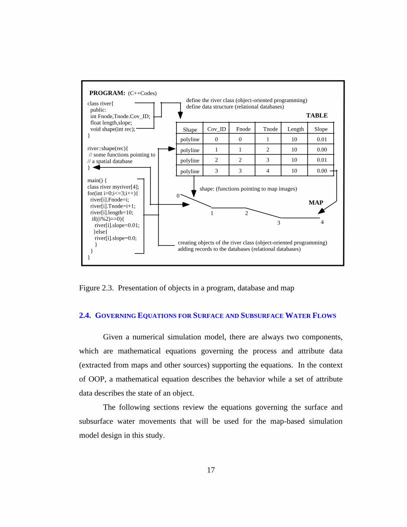
Figure 2.3 shows how an object is defined and referenced in an object-oriented
programming language, in a relational database, and on a map. C++ is used here
to illustrate how an object is defined in an object-oriented programming language.
As stated above, an object is defined by the equation: object = state +
behavior. The behavior of an object is governed by some equations. Equations
are usually translated into element functions. In the same way, states of an object
are defined as variables of a class. The program section in Figure 2.3 illustrates
how a class is defined and objects generated in C++. In this example program,
objects are created in two steps. First, a class is defined and functions declared,
and then the instances (objects) of the class are generated. These two steps are
analogous to the actions of creating a database structure (template) and adding
records to the database. When a GIS map is constructed, a relational database is
also created to store the spatially-referenced data sets. Such databases appear as
feature attribute tables (FTAB) in the ArcView program. In the database of a
GIS map, one field is used to hold the pointers to the geographical features on the
map. In a class, states (variables) and behaviors (element functions) can be
defined as either private or public. A private variable/function is accessible only
by other elements of the same object while a public variable/functions can be
called by other objects. The distinction of private and public types of functions
and variables provides a mechanism for programs to control the messages
(requests) exchanged between objects.
17
class river{ public: int Fnode,Tnode.Cov_ID; float length,slope; void shape(int rec);}
river::shape(rec){ // some functions pointing to// a spatial database}
main() {class river myriver[4];for(int i=0;i<=3;i++){ river[i].Fnode=i; river[i].Tnode=i+1; river[i].length=10; if((i%2)==0){ river[i].slope=0.01; }else{ river[i].slope=0.0; } }}
Shape Fnode
0
1
2
3
Tnode
1
2
3
4
Length
10
10
10
10
Slope
0.01
0.00
0.01
0.00
define the river class (object-oriented programming)define data structure (relational databases)
creating objects of the river class (object-oriented programming)adding records to the databases (relational databases)
polyline
polyline
polyline
polyline
0
1 2
3 4
shape: (functions pointing to map images)
PROGRAM:
MAP
TABLE
(C++Codes)
Cov_ID
0
1
2
3
Figure 2.3. Presentation of objects in a program, database and map
2.4. GOVERNING EQUATIONS FOR SURFACE AND SUBSURFACE WATER FLOWS
Given a numerical simulation model, there are always two components,
which are mathematical equations governing the process and attribute data
(extracted from maps and other sources) supporting the equations. In the context
of OOP, a mathematical equation describes the behavior while a set of attribute
data describes the state of an object.
The following sections review the equations governing the surface and
subsurface water movements that will be used for the map-based simulation
model design in this study.

18
2.4.1. Equations Related to the Surface Water Flow Simulation
Two types of models are considered for surface water flow simulation:
one for stream flow and one for overland flow. Figure 2.4 shows the data flow
path on the map-based surface water flow simulation model.
As it can be seen from Figure 2.4, six procedures are used to process and
convert the rainfall data sets and produce flow time-series the river section nodes.
Rainfall time-seriesdefined on rain-gagestations (point-cov.)
Interpolation procedure
Rainfall time-series definedon soil-water balance modelcomputation units
Soil-water balance model
Water surplus definedon soil-water balancemodel’s computaion units
Conversion procedure
Water surplus defined onsubwatershed polygonsused for flow simulation
Convolution procedure
Local runoff contributiontime series defined onsubwatershed polygons
River routing procedures
River flow time seriesdefined on river nodes
Postprocessing procedures
1
2
3
4
5
6
Figure 2.4. Data flow path in the map-based surface water flow simulation model
The input data for this map-based surface water flow simulation model are
a set of rainfall time-series defined on the rain-gauge stations on the study area.

19
These rainfall time-series are interpolated to each of the computation units of a
soil-water balance model (procedure 1). The interpolated rainfall time-series are
used by the soil-water balance model (procedure 2) to produce soil-water surplus
time-series defined on the computational units of the soil-water balance model. If
subwatershed polygons are used as the computational units of the soil-water
balance model, the water-surplus time-series can be used directly by a convolution
procedure (procedure 4) to produce the local runoff contributions. Otherwise, a
conversion procedure (procedure 3) has to be applied to convert the water-surplus
from a set of time-series defined on the soil-water balance units to another set of
time-series defined on the subwatershed polygons before the convolution
procedure can be applied. The convolution procedure produces a flow time-series
representing the runoff contribution of each subwatershed. The river routing
procedures (procedure 5) together with the river network analysis procedure (to be
discussed in Chapter Three) are then applied to generate flow time-series defined
at the starting and ending points of each river line section in the river network.
In the following sections, the equations governing the soil-water balance
computation, water surplus to runoff conversion, river flow routing, and the
methods for converting time-series data between different spatial features are
discussed.
2.4.1.1. The Soil -Water Balance Model
A soil-water balance model estimates the soil-water surplus given a
precipitation time-series, soil-water holding capacity information, and potential
evaporation information. The surplus is defined as water which does not
evaporate or remain in soil storage and is available to generate surface and
subsurface runoff. Surplus can be estimated using a simple bucket model

20
(Thornthwaite, 1948, Willmott et al., 1985, Mintz and Serafini, 1993). In the
simple bucket model, the basic equations for calculating surplus are:
w(t)
t
w(t -1)
t+ P(t) E(t)
∆ ∆= −
(2.1a)
S(t)(w(t) w )
t; w(t) = w if w(t) > w
S(t) = 0; w(t) = w(t) if w(t) w
** *
*
=−
≤∆ (2.1b)
where,
S(t) = surplus [LT-1],
P(t) = precipitation [LT-1],
E(t) = evaporation [LT-1],
w(t) = soil moisture storage of the computation unit at time step t [L],
w* = soil-water holding capacity [L],
∆t = computation time step [T].
• Constructing a Precipitation Surface From Rainfall Data
The precipitation data are usually available in the form of time-series data
associated with the locations of rain-gauge stations. These rainfall time-series
need to be spatially interpolated to the cells on which equation 2.1 will be applied.
There are many algorithms available to perform spatial interpolation, such as the
methods of triangulated irregular network (TIN), Kriging, Thiessen polygons,
two-dimensional spline, and inverse-distance weighting. Procedures for applying
these interpolation methods can be found in numerous publications, e.g. the series

21
of ARC/INFO User’s Guide, (ESRI, 1992). When the method of TIN is used for
the interpolation, a TIN is first constructed from the point coverage of rain-gauge
stations. The ARC/INFO function TINLATTICE can then be used to interpolate
the rainfall values to the centers of soil-water balance computation units.
• Computing the Evaporation
Three types of equations are available for potential evaporation
estimations (Applied Hydrology, pp82-86) and they are listed below.
(1) Energy method:
Er =Rn
lv ⋅ ρw(2.2a)
where,
Er = the estimated evaporation rate[LT-1],
Rn = net radiation flux {200 W/M2}={200 J/SM2},
lv = latent heat of water vaporization{2441 KJ/Kg},
ρw = water density{997 Kg/M3}.
The numbers listed in {} are used to provide a sense of the parameter's normal
value range.
(2) Aerodynamic method:
Ea = B(eas − e) (2.2b)
where,

22
Ea = the estimated evaporation rate[mm],
eas = vapor pressure at water surface {3167 Pa at 25oC},
e = vapor pressure of the air,
B =0.622k2ρau2
pρw[2ln(z2 / zo )]
k = Von Karman’s constant, k = 0.4,
ρa = air density, { ρa kg m= 119 3. / at 25oC},
p = ambient air pressure, {p = 101.3 kPa at25oC},
u2 = air velocity at elevation Z2,
Z0 = reference height of boundary.
(3) Combined aerodynamic and energy method:
E =∆
∆ + γEr +
γ∆ + γ
Ea (2.3)
where,
∆ =des
dT=
4098es
(237.3 + T)2 = vapor pressure gradient with temperature,
γ = psychometric constant.
In this research, the energy method (Equation 2.2a) is used to estimate the
potential evaporation in the simple bucket model.
• Setting the Model’s Initial Conditions
As can be seen from Equation 2.1, computation of soil-moisture surplus is
an iterative procedure, and the initial soil moisture storage w(t=0) is needed

23
before the computation can start. Since the initial soil moisture storage is
typically unknown, the following water balancing procedure is applied to force
the net change in soil moisture from the beginning to the end of a specified
balancing period to zero, i.e., w(0) − w(n +1) < ξ , where n is the number of time
steps of the computation period, and ξ is a user specified tolerance (ξ = 0.1 mm
is used in the research). Starting with the initial soil moisture being set to the
water-holding capacity, budget calculations are made to until t=n+1. w(0) is then
set to w(n+1) to start another budget calculation circle until the condition
w(0) − w(n +1) < ξ is satisfied.
2.4.1.2. Converting Time-Series between Different Spatial Features
The soil-water balance model produces a time-series of water surplus
defined on the model’s computation units. Because the units used for the soil-
water balance usually are not the subwatershed polygons used for surface water
flow simulation, the time-series of water surplus values needs to be converted so
that the values are defined on the subwatersheds. This section describes the
procedure for the conversion of a data set defined on one type of spatial features
to those defined on another set of spatial features.
To illustrate the procedure, assume P is a set of data defined on In-
Coverage and is to be converted so that it is defined on Out-Coverage. The first
step of the data converting procedure is to use the INTERSECT function provided
by the ARC/INFO to establish the spatial relationships between In-Coverage and
Out-Coverage. The INTERSECT operation produces a new Intersect-Coverage.
As shown in Figure 2.5, nine components of P on the In-Coverage will become
four components defined on Out-Coverage after the conversion. Assume the area
on each feature on the In-Coverage to be A1, A2, ..A9, and the areas of map units

24
on the Intersect-Coverage to be Iij, with i representing the In-Coverage ID and j
representing the Out-Coverage ID. Let OP and IP represent the components of P
defined on the Out-Coverage and defined on the In-Coverage, respectively. The
equations used for OP1 can then be written as:
OP1 =IP1 ⋅ I11 + IP2 ⋅ I21 + IP4 ⋅ I41 + IP5 ⋅ I51
I11 + I21 + I 41 + I51
(2.4a)
if P is an intensive property, and
OP1
= IP1
⋅I11A
1+ IP
2⋅
I21A2
+ IP4
⋅I42A
4+ IP
5
I51A
5(2.4b)
if P is an extensive property.

25
1 2 3
4 5 6
7 8 9
In-Coverage
P={IP1,IP2,IP3,IP4,IP5,IP6,IP7,IP8,IP9}
1 2
3 4
Out-Coverage
P={OP1,OP2,OP3,OP4}
I11 I21
I41 I51
Intersect-Coverage
If P is an intensive property, then:
If P is an extensive property, then:
OP1 = IP1 ⋅I11A1
+ IP2⋅I21A2
+ IP4 ⋅I42A4
+ IP5
I51A5
OP1 =IP1 ⋅I11 + IP2 ⋅I21 + IP4 ⋅I41 + IP5 ⋅I51
I11 + I21 + I41 + I51
Figure 2.5. Converting data sets between different spatial features
In general, the conversion equations can be written as:
OPj = IPii
∑ ⋅ Iij (2.5a)
if P is an intensive property, and
OPj = IPii
∑ ⋅Iij
Ai
(2.5b)

26
if P is an extensive property, where,
OPj = property P defined on unit j at the Out-Coverage,
IPi = property P defined on unit i at the In-Coverage,
Iij = the area of unit i on the In-Coverage that intersects with unit j on the
Out-Coverage,
Ai = the area of unit i on the In-Coverage. To convert time-series data,
equation 2.5 needs to be applied to the data at each time step.
2.4.1.3. Convolution Procedure Used To Compute Local Runoff
The time-series representing the local runoff of a subwatershed to the river
network (PFlow(t)) can be calculated from the time-series of water-surplus
(SurpF(t)) defined on the subwatershed. In the following text, when referring to a
time-series in general, for example, PFLOW, the notation PFlow(t) will be used
and when referring the same time-series related to a specific spatial feature, the
notation PFlowit will be used; a subscript (i) indicates the spatial feature index
and a superscript (t) indicates the time index. Because the water surplus can reach
a river section through either overland flow or through subsurface flow, the
portion of surplus flow that reaches a river section through overland flow will be
referred to as SFlow(t) and the portion that goes into the subsurface before it
reaches the river section will be termed as OFlow(t) (Figure 2.6). Based on this
assumption, we have:
PFlow(t) = SFlow(t) + OFlow(t) (2.6)
The overland flow portion (SFlow(t)) can be computed from SurpF(t)
using equation (Olivera and Maidment, 1996):

27
SFlowit = SurpFi
t −k
k= 0
min( t, N)
∑ (1 −α i) ⋅Uik (2.7)
where,
SFlowit = local surface water flow contribution (m3/s), of subwatershed i at
time step t,
SurpFit −k = soil moisture surplus (m3/s) of subwatershed i at time step t-k,
Uik = k-th component of the response function of PFlowi
t on SurpFit ,
αi = the fraction of surplus that goes to subsurface, (0 ≤ αi ≤ 1),
N = total number of components in the response function Uik . The
response function of PFlowit on SurpFi
t used in this study is given below:
U
k DikviTi
( ) k= , , ....Nik
(kviTi
)
DikviTi
= −−1
2
1 2 31 2
4π
exp (2.8)
where,
k =1,2,3...N, the index of components in the response function,
Di = dispersion coefficient for subwatershed i, Dispersion coefficient is
used to measure the degree of the spreading of overland water flow
over time.
Vi = average overland flow velocity for subwatershed i (m/s),
Ti = average overland flow time for subwatershed i (s).

28
Figure 2.6 is constructed to illustrate how the parameters of Equation 2.8
can be estimated. In Figure 2.6, subwatershed i is composed of a number of cells
(elements) and for a given element e, its flow length le can be calculated using the
GRID module in ARC/INFO. The flow time of water from element e to the outlet
of the subwatershed can be estimated by dividing the flow length le by the average
flow velocity ve, which could estimated from the topology and land cover
information of the subwatershed. The average overland flow time for
subwatershed Pi is then computed using:
Ti = te ⋅Ae
Aie =1
Ne
∑ (2.9)
where, Ae and Ai are the areas of element e and subwatershed i,
respectively.
When all the elements forming the subwatershed have the same size,
which is the case when the GRID module is used, Equation 2.9 becomes:
Ti =1
Ne
tee=1
Ne
∑ (2.9a)
where, Ne = the number of elements in the subwatershed.
Using the Zonalstats function provided by the GRID module in
ARC/INFO, the average overland flow length li and standard deviation σ i of the
flow length for subwatershed Pi can also be calculated. With these two
parameters, the dispersion coefficient for the subwatershed Pi can be computed
using:

29
Di =σ i
2
2(li2 )
(2.10)
where,
σ i = the standard deviation of the flow length for subwatershed Pi,
li = the average overland flow length for subwatershed Pi.
The subsurface water flow component of PFlow(t) is considered to be
going through an imaginary under-ground-reservoir whose flow can be simulated
using a linear-reservoir-model (Equations 2.11 and 2.12):
OFlowit = Si
t −1 / Ki (t = 1,2,3,....) (2.11)
Sit = Si
t −1 + (SurpFit ⋅ αi −OFlowi
t ) ⋅ ∆t (2.12)
where,
OFlowit = PFlow’s subsurface component at time step t, on polygon i
[L 3T-1],
Sit = storage of the underground reservoir at time step t, on polygon i [L3],
Ki = the linear reservoir constant [T].
After the components simulating surface and subsurface water flows are
computed, the local flow contribution of subwatershed i at time step t is computed
using Equation 2.6.

30
Subwatershed Pi
le, ve, te=le/ve
Element e
SurpF(t)
OFlow(t)
SFlow(t) PFlow(t)
SurpF(t) to PFlow(t) conversion
Subsurface reservoir
Figure 2.6. Converting SurpF(t) to PFlow(t)
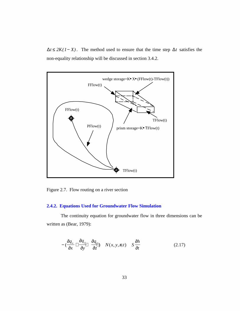
2.4.1.4. Flow Routing on a River Section
The flow in a river section shown in Figure 2.7 can be simulated using the
Muskingum or Muskingum-Cunge method (McCarthy, 1938, Cunge,1969, Chow
et al., 1987). The Muskingum method is based on the principle of continuity and
a relationship between discharge and the temporary storage of excess volumes of
water in a river section during the simulation period. The principle can be
expressed as:
dS
dtI t Q t= −( ) ( ) (2.13)
where,
S = the volume of water in storage in a river section,

31
I(t) = water inflow time-series (hydrograph) of the river section [L3T-1],
Q(t) = water outflow time-series of the river section [L3T-1].
In deriving the flow routing formula for the Muskingum method, it is
assumed that the storage volume in a river section (Figure 2.7) is composed of
two portions: a wedge storage and a prism storage. It is further assumed that the
cross-sectional area of the water flow is directly proportional to discharge into the
section, the volume of prism storage is K•TFlow(t) and the volume of wedge
storage is K•X•(FFlow(t)-TFlow(t)), where K is a proportionality coefficient and
X is a weighting factor showing the relative importance of FFlow(t) and TFlow(t).
With these assumptions, the total storage of the section can be written as:
S t K TFlow t K X FFlow t TFlow t( ) ( ) ( ( ) ( ))= ⋅ + ⋅ ⋅ − (2.14)
The formula of Muskingum routing method is derived by expressing the
storage change of the section between time step t and t-1 in terms of FFlow(t) and
TFlow(t) using Equation 2.14. Muskingum-Cunge method is derived based on
the Muskingum method taking into consideration the lateral flow (PFlow(t)).
Detailed descriptions of Muskingum-Cunge flow routing method can be found in
Applied Hydrology (Chow et al., 1987), Hydrology for Engineers (Linsley et al,
1982), and Handbook of Hydrology (Maidment, 1993).
The Muskingum-Cunge flow routing method is described by the following
equation:
TFlow t C FFlow t C FFlow t
C TFlow t C
( ) ( ) ( )
( )
= ⋅ + ⋅ −+ ⋅ − +
1 2
3 4
1
1 (2.15)

32
where,
TFlow(t) = flow time-series at the To-Node of a river line,
FFlow(t) = flow time-series at the From-Node of a river line,
C1, C2, C3, C4 = coefficients related to river and flow characteristics.
These coefficients are computed using equations given below:
C1 =∆t − 2KX
2K(1 − X) + ∆t(2.16a)
C2 =∆t + 2KX
2K(1− X ) + ∆t(2.16b)
C3 =2K(1 − X) − ∆t
2K(1 − X) + ∆t(2.16c)
C4 =PFlowi
t − DFlowit − Lossi
t
2K(1 − X) + ∆t(2.16d)
Kx
c=
∆, K is a storage constant [T], (2.16e)
X =1
2−
Avg(TFlow, FFlow)
2c B Se∆X (2.16f)
X = a weighting factor showing the relative importance that FFlow and
TFlow have on the river section’s storage,
∆x = the length of the river section, [L]
c = kinematic wave velocity [LT-1],
B = cross-sectional top width associated with average of TFlow and
FFlow,
Se = the energy slope, and∆X = length of a river section.
To ensure the stability of the flow routing, C3 needs to be non-negative.
From equation 2.16c, it can be seen that in order for C3 ≥ 0 , we need to have:
33
∆t ≤ 2K(1− X) . The method used to ensure that the time step ∆t satisfies the
non-equality relationship will be discussed in section 3.4.2.
FFlow(t)
TFlow(t)
PFlow(t)
TFlow(t)
FFlow(t)
wedge storage=K•X•(FFlow(t)-TFlow(t))
prism storage=K•ΤFlow(t)
Figure 2.7. Flow routing on a river section
2.4.2. Equations Used for Groundwater Flow Simulation
The continuity equation for groundwater flow in three dimensions can be
written as (Bear, 1979):
− + + + =( ) ( , , , )∂∂
∂∂
∂∂
∂∂
q
x
q
y
q
zN x y z t S
h
tx y z (2.17)

34
where,
h = piezometric head of the aquifer [L],
N(x,y,z,t) = a point source (or point sink when N is negative) [T-1], at
point (x,y,z),
S = ρg(α + β )= specific storage [L-1],
α =−1
1 ndndp
= the matrix compressibility [M-1LT2],
βρ
ρ= 1 ddp
= the water compressibility [M-1LT2],
n = the porosity of the aquifer,
qx , qy, qz = the components of the specific discharge vector r q [LT-1] in x,
y, z directions. r q can be computed using Darcy’s law:
r q = −K grad h = −K∇h (2.18)
where,
K = the hydraulic conductivity of the aquifer [LT-1],
∇ = (
∂∂x
r i +
∂∂y
r j +
∂∂z
r k ) is gradient operator.
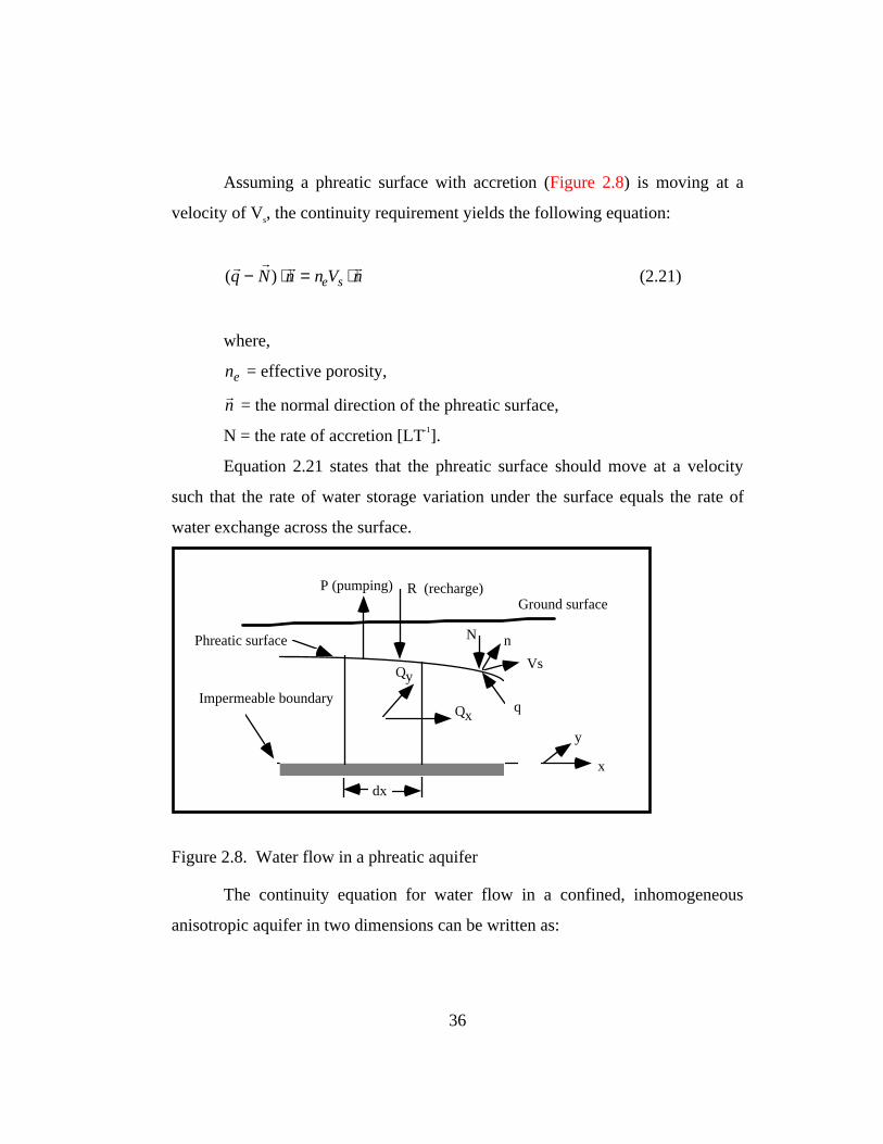
The continuity equation for groundwater flow in a phreatic aquifer in two
dimensions (Figure 2.8) can be written as:
− + + − =( )∂∂
∂∂
∂∂
Q
x
Q
yR P S
h
tx y
(2.19a)
or
∂∂
∂∂
∂∂
∂∂
∂∂x
K hh
x yK h
h
yR P S
h
tx y( ) ( )+ + − = (2.19b)

35
where,
Kx and Ky are the hydraulic conductivity in x and y directions,
Qx = −Kxh∂h
∂x = the discharge per unit width of the aquifer in x direction
[L2T-1],
Qy = −Kyh∂h
∂y = the discharge per unit width of the aquifer in x direction
[L2T-1],
R = R(x,y,t) = recharge to the aquifer [LT-1],
P = P(x,y,t) = pumpage from the aquifer [LT-1]
S = specific storage.
Equations 2.19a and 2.19b can be derived by integrating Equation 2.17
over the Z dimension while taking into consideration (1) the Dupuit horizontal
flow assumption, (2) Leibnitz rule and (3) the boundary condition at the phreatic
surface. Detailed derivation procedure can be found in the book Hydraulics of
Groundwater (Bear, 1979). A brief description of Leibnitz rule and the boundary
condition at the phreatic surface is given here.
For an aquifer of thickness B = Z2(x, y, t) − Z1(x, y,t) and given a scalar
h(x,y,z,t)defined on the aquifer, according to Leibnitz rule, we have:
∂∂t
hdz =∂∂t
(Bh ) =∂h
∂tdz + h Z2
∂Z2
∂tZ1
Z2
∫Z1(x,y,t)
Z 2(x ,y,t )
∫ − h Z1
∂Z1
∂t(2.20)
where, hB
hdzZ
Z
= ∫1
1
2
.
36
Assuming a phreatic surface with accretion (Figure 2.8) is moving at a
velocity of Vs, the continuity requirement yields the following equation:
(r q −
r N ) ⋅
r n = neVs ⋅
r n (2.21)
where,
ne = effective porosity,
r n = the normal direction of the phreatic surface,
N = the rate of accretion [LT-1].
Equation 2.21 states that the phreatic surface should move at a velocity
such that the rate of water storage variation under the surface equals the rate of
water exchange across the surface.
Phreatic surface
R (recharge)
dx
Qx
Qy
Impermeable boundary
P (pumping)
x
y
Ground surface
n
Vs
q
N
Figure 2.8. Water flow in a phreatic aquifer
The continuity equation for water flow in a confined, inhomogeneous
anisotropic aquifer in two dimensions can be written as:

37
∂∂
∂∂
∂∂
∂∂
∂∂x
Th
x yT
h
yR P S
h
tx y S( ) ( )+ + − = (2.22)
where,
h = h(x,y,t) = piezometric head of the aquifer at point x,y [L],
Tx = Tx (x,y) = aquifer transimisivity in x direction [L2T-1],
Ty = Ty (x,y) = aquifer transimisivity in y direction [L2T-1],
SS = aquifer storativity. If the aquifer is inhomogeneous and isotropic, we
have Tx = Ty = T(x,y). If the aquifer is homogeneous and isotropic, we have Tx =
Ty = T.
Equation 2.22 can also be derived by integrating equation 2.17 over the
aquifer thickness while taking into consideration of Leibnitz rule and aquifer’s top
and bottom boundary conditions.
To solve Equation 2.19 (or Equation 2.22) numerically, the first step is to
discretize the region of interest, i.e. to replace the continuous region for which a
solution is desired by an array of points. These points are usually the center
points of grid cells or corner points of a grid. Then either a finite element or a
finite difference method is applied to these points to convert the differential
equation into a set of linear equations. This set of linear equations are then solved
by some appropriate solver. Detailed discussions on the subject of solving the
equations using finite element and finite difference methods can be found in the
textbooks by Becker et al. (1981), Remson et al. (1971), Desai (1979), Wang and
Anderson (1982), Huyakorn and Pinder (1983), and numerous articles, e.g.,
Pinder and Gray (1977).
Because solving the groundwater flow equation in form of the equation
2.19 or 2.22 is complicated and computational intensive, models based on this

38
type of equations such as Modflow (McDonald and Harbaugh, 1988) and
GWSim4 (TDWR, 1974) are usually self-contained. Therefore, it is difficult to
fully integrate this type of groundwater model with a geographic information
system (GIS).
To avoid this difficulty, a map-based groundwater simulation model will
be constructed. The map-based model is constructed on a polygon and the
polygon’s boundary line coverages. This model simulates groundwater flow by
alternatively applying the continuity equation to the polygon objects and the
momentum equation to the polygon boundary line objects. This section describes
the concept of the map-based groundwater simulation model. A detailed model
constructing and programming procedure are discussed in Chapter Four.
Figure 2.9 illustrates the concept of the map-based groundwater
simulation model. The continuity equation (discretized in time) derived from
Equation 2.19 or Equation 2.22 for a polygon object in Figure 2.9 can be written
as:
∆tt ⋅ Ai ⋅ Rit − Pi
t − Qit( )[ ]+ Vij
t
j∑ = A i ⋅Si ⋅(hi
t − hit−1 ) (2.23)
where,
∆tt = time interval at time step t,
Ai = area of cell i,
Rit , Pi
t , and Qit = recharge, pumpage, and discharge of the aquifer under
cell i at time step t, respectively, [LT-1],
Vijt = volume of water that enters cell i through boundary j at time step t
[L 3], The computation ofVijt is based on the momentum equation

39
(Darcy’s Law) and a line integration technique to be discussed in
Chapter Four.
Si = the storativity (for a confined aquifer) or the specific storage (for a
phreatic aquifer, of cell i [L0T0],
hit = water level of cell i at the end of time step t [L],
hit −1 = water level of cell i at the end of time step t-1 [L].
Also in Figure 2.9, the momentum equation in the form of Darcy's law can
be applied to each boundary line of the polygon objects and for a given boundary
line object, the momentum equation can be written as:
r q ij
t = −kij
dh
ds
r s ≈ −kij
h jt −1 − hi
t −1
∆sij
r s (2.24)
where,
kij = hydraulic conductivity between polygons i and j [LT-1],
r q ij
t = flux of water [LT-1] across the boundary line between polygons i & j
at time step t,
r s = a unit vector pointing from the center of polygon i to that of polygon
j,
∆sij = distance between the centers of polygons i and j [L],
hjt −1, hi
t −1 = water levels of polygons j and i at time step t-1 [L].
The logic of the map-based model is simple. Given the initial head levels
of the polygons, Equation 2.24 is applied to each boundary line object to compute
groundwater flow across each boundary line object. As a result of this
computation, the water volumes (Vijt ) transported in and out of each polygon

40
object in the first time step are obtained. With Vijt known, the continuity equation
(Equation 2.23) is then applied to each polygon object to calculate the water level
at the end of first time step. This procedure of alternatively applying the
momentum equation to line objects and the continuity equation to polygon objects
will be repeated until the end of the simulation period.
•
•
•
•
•
•
•
•
••
•••
Applying the continuity equation(Equation 2.23) to the volume ofwater in each polygon
Applying the momentum equation(Darcy’s Law ) to each boundaryline of the polygons (Equation 2.24)
i j
Figure 2.9. The conceptual design of a map-based groundwater model
2.5. CHAPTER SUMMARY
As it can be seen from this section, the surface water flow processes
(overland flow, river flow etc.) can be simulated one region at a time when the
water exchange between subwatersheds can be represented by a set of time-series
data. For this reason, surface water flow processes for a subwatershed can be
simulated by making a sequence of functional calls in a certain order.

41
Also, it can be seen from the equations presented above that the data
supporting these equations can be categorized into two types, static and dynamic.
Static data do not change throughout the whole simulation period, while dynamic
data vary from one time step to another. The dynamic data type itself can be
further divided into two types, predetermined and run-time determined.
Predetermined dynamic data, such as rainfall time-series, are known before
running the model. Run-time determined dynamic data, such as the groundwater
flow velocity field used to compute Courant number ( CoV t
x=
⋅ ∆∆
) for a given
time step, are not known until the simulation of previous time steps is completed.
The reason for making this data classification is that different types of data may
require different data structures for efficient data storage and retrieval. Detailed
discussions about the treatments of different data types are presented in Chapter
Three.
The map-based groundwater simulation model is constructed by applying
the finite difference form of the continuity equation (Equation 2.23) to the water
volumes of polygon objects and the finite difference form of the momentum
equation (Equation 2.24) to the polygon boundary line objects. Because the
spatial features are grouped into line and polygon coverages in ARC/INFO,
separately applying these two equations to these two types of objects greatly
simplifies the solution procedures.

42
Chapter Three. A Map-Based Surface Water Flow Simulation Model
3.1. INTRODUCTION
Through the construction of a map-based surface water flow simulation
model (SFlowSim) for the Niger River Basin in West Africa, this chapter
demonstrates how the three elements ( maps, data sets, and programs) of a
simulation model are integrated.
The map-based surface water flow simulation model can be used for the
water resources assessment and management of a river basin. The model can be
applied to any area where a digital elevation model (DEM) is available or to a
region whose river basin polygons and river lines are available. Listed below are
the tasks that this model can accomplish:
• Simulate river flow time-series based on precipitation defined on watershed
polygons or water surplus defined on soil units. After applying the
simulation model to a river basin, the flow rates are available at the From-
Node and To-Node (termed FFlow and TFlow, respectively, in the model)
of each river line. The From-Node and To-Node represent the starting and
ending points of a river section line (Figure 3.1). The Post-processor of the
simulation model can also interpolate flow rates to any user defined points
along the river section.
• Estimate the flow contribution of each subwatershed (termed PFlow in the
model).
• Allow reservoir objects to be added to a river section and simulate their
effects.

43
• Allow diversion points to be set on a river section and simulate their effects
on downstream river flows.
• Plot a longitudinal flow profiles along a user specified river section.
• Plot the flow time-series (FFlow(t) and TFlow(t)) of a river section or the
flow contribution time-series of a subwatershed.
• Allow a user to clip out part of a river basin to create a sub-model so that a
more detailed study of the selected subregion can be performed.
• Optimize model parameters to facilitate the calibration of the simulation
model.
• Allow a user to modify the modeling conditions directly from the model
base maps.
• Integrate with the map-based groundwater simulation model to simulate the
flow interaction between surface and subsurface water flows.
Three classes of objects are essential for this map-based surface water flow
simulation model. They are (1) a line class created to represent river sections, (2)
a polygon class created to represent the subwatersheds associated with the river
sections, and (3) a point class created to represent reservoirs or diversion points
within any river section. Each river section is an instance (object) of the line
class, with its states being stored in a line value attribute table and its behavior
described by some flow routing equations. As each record is added to the line
attribute table, a new river section object is created. The same thing can be said
for the river basin polygon and reservoir point classes.

44
GC=1GC=2
1
23
(1) Assuming single-cell polygons 1, 2, 3, all have a Grid-Code (GC) value of 1(2) Running ARC/INFO DISSOLVE function will dissolve cell 1 with subwatershed GC=1, but not single-cell polygon 2, and 3, because they don’t share any common boundary lines with subwatershed GC=1.(3) After running the AVENUE program SFdslv.pre, single-cell polygons 2, and 3 will have their Grid-Code reassigned to 2.(4) Running ARC.INFO DISSOLVE function again will dissolve cell 2, and 3 with the subwatershed GC=2, because they now share at least one common boundary line.
GC=Grid-Code
Single-cell polygons
Subwatershed •
•
From-Node
To-Node
River section
Figure 3.1. Solving the problem of one-line-to-many-polygons
3.2. MODEL CONSTRUCTION PROCEDURE
Based on their functions, the programs in the map-based surface water
flow simulation model can be grouped to form three modules: pre-processor,
processor and post-processor. The pre-processor is used to create the model
objects, construct model base maps, create time-series data tables and process
time-series data. The processor is used simulate water flow on the rivers and
subwatersheds. The post-processor is used to analyze and display model results.
The post-processor also contains utility programs that can be used to modify
model maps and modeling conditions and to perform map operation and database

45
management tasks. Figure 3.2 shows the components of the map-based surface
water flow simulation model (SFlowSim) and its construction procedure. The
following section discusses the functions of the pre-processor and the construction
of model maps.
3.2.1. Preparing Maps for a Map-Based Simulation Model
The maps (river and basin coverages) of a map-based simulation model
are constructed by applying the river basin delineation procedure (Maidment,
1994) to a digital elevation model (DEM). As a result of running this delineation
procedure, two map coverages are produced. One is a line coverage representing
the rivers and the other one is a polygon coverage representing the drainage areas
of the rivers. Figure 2.2 shows the rivers and subwatersheds of the Guadalupe
River Basin created by delineating a 3’’ (with a grid cell size of 92.7x92.7 meters)
DEM of the region. These river line and subwatershed polygon coverages are
imported into an ArcView project and processed by a set of AVENUE programs
(pre-processor). The processed river sections form a river network whose
members have a one-to-one relation with the subwatershed polygons associated
with the river network. The pre-processor programs and simulation model’s basic
assumptions are discussed below.

46
Regional DEM lattices(Raster based GIS)
Watershed delineationprocedure
River line and watershedpolygon coverages(Vector based GIS)
Map-operating procedures * create river line object * create watershed object * construct stream network * establish one-to-one link between river lines and watershed polygons
Suitable for spatial analysis
Suitable for network analysis
Map-Based Surface Flow Simulation Model Processor
Pre-processor
Flow distribution display
Constructor of the riverflow diversion objects
Constructor of the dam/reservoir objectsFlow-check point constructor
Baby-model constructorOptimization program formodel parameter-fitting
Utility programsPost-processor
Avenue programsSpatially-referencedtime series data sets
Base Maps
Figure 3.2. Components of the map-based model SFlowSim
3.2.2. Basic Assumptions for a Map-Based Simulation Model
A map-based surface water flow simulation model is constructed based on
the following assumptions about the river network and subwatersheds:
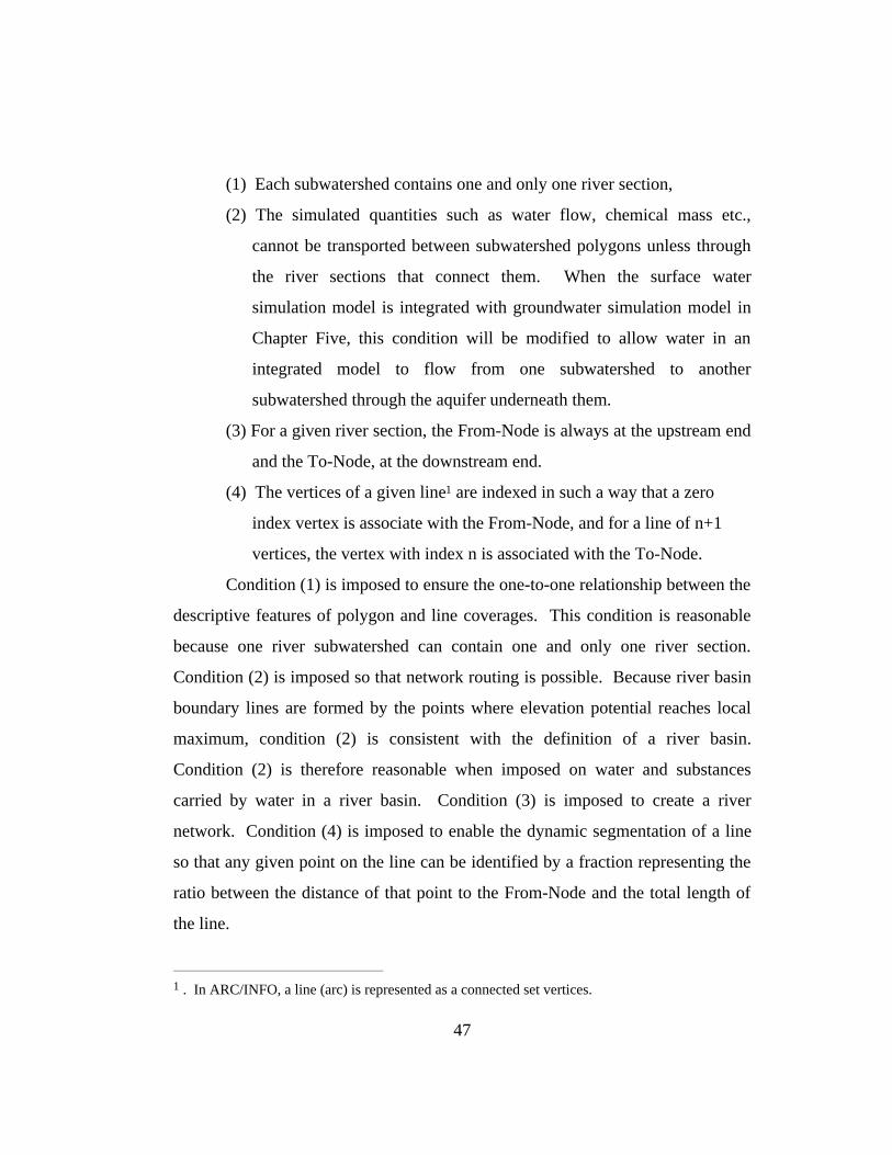
47
(1) Each subwatershed contains one and only one river section,
(2) The simulated quantities such as water flow, chemical mass etc.,
cannot be transported between subwatershed polygons unless through
the river sections that connect them. When the surface water
simulation model is integrated with groundwater simulation model in
Chapter Five, this condition will be modified to allow water in an
integrated model to flow from one subwatershed to another
subwatershed through the aquifer underneath them.
(3) For a given river section, the From-Node is always at the upstream end
and the To-Node, at the downstream end.
(4) The vertices of a given line1 are indexed in such a way that a zero
index vertex is associate with the From-Node, and for a line of n+1
vertices, the vertex with index n is associated with the To-Node.
Condition (1) is imposed to ensure the one-to-one relationship between the
descriptive features of polygon and line coverages. This condition is reasonable
because one river subwatershed can contain one and only one river section.
Condition (2) is imposed so that network routing is possible. Because river basin
boundary lines are formed by the points where elevation potential reaches local
maximum, condition (2) is consistent with the definition of a river basin.
Condition (2) is therefore reasonable when imposed on water and substances
carried by water in a river basin. Condition (3) is imposed to create a river
network. Condition (4) is imposed to enable the dynamic segmentation of a line
so that any given point on the line can be identified by a fraction representing the
ratio between the distance of that point to the From-Node and the total length of
the line.
1 . In ARC/INFO, a line (arc) is represented as a connected set vertices.

48
3.2.3. Construction of Basic Maps
The vector GIS coverages created by the grid-based watershed delineation
procedure (Maidment, 1994) may not meet the assumptions listed above because
the raster-to-vector conversion procedure does not always ensure a one-to-one
relationship between river lines and subwatershed polygons. The problems to be
corrected are usually one-line-to-many-polygons and one-polygon-to-many-lines.
The problem of one-line-to-many-polygons is usually caused by the existence of
single-grid-cell (single-cell) polygons.
Figure 3.1 shows an example of the problem created by the single-cell
polygons. To correct the problem, these single-cell polygons need to be
eliminated by dissolving them into the appropriate subwatershed polygons.
ARC/INFO provides a DISSOLVE function that will dissolve polygons that (1)
have the same value of a given field (e.g. Grid-Code) and (2) share a boundary
line. For the single-cell polygons that have the same value of Grid-Code with a
subwatershed polygon but do not share any boundary lines with the subwatershed,
an AVENUE program is written to reassign to each of these single-cell polygons
the Grid-Code of a subwatershed that shares the same boundary line with it. The
AVENUE program will first identify and put all single-cell polygons into a list.
Then for each member of the list, the program uses LPoly_ and RPoly_ attributes
of the polygon’s boundary lines to identify one of its adjacent subwatershed
polygons, whose Grid-Code value is then assigned to that of the single-cell
polygon. The fields LPoly_ and RPoly_ of a line (arc) attribute table hold the
machine-assigned IDs of left polygon and right polygon, respectively. After all
the single-cell polygons have their Grid-Code reassigned, the DISSOLVE
function of the ARC/INFO program is reapplied with Grid-Code as the dissolving

49
value to eliminate the single-cell polygons. This procedure solves the problem of
one-line-to-many-polygons.
The problem of one-polygon-to-many-lines can occur in the situations of
(1) split river line segments in a single subwatershed, (2) multiple river line
segments within one subwatershed, and (3) incorrect node indexing on the river
line coverage. Figures 3.4 and 3.5 illustrate the examples of these situations. One
of the tasks of the pre-processor is to eliminate the problem of one-polygon-to-
many-lines by running a series of map-processing programs to modify the
ARC/INFO coverages created by the watershed delineation procedure. After
modification, these two coverages (river line and subwatershed polygon) will
meet the four conditions listed in section 3.2.2. and be ready for use by the map-
based flow simulation model. The functions of each program in the pre-processor
are described below:
1. Creating River Line and Subwatershed Polygon Objects [SFmdfld.pre]
This program adds attributes to the standard ARC/INFO arc attribute table
(AAT) and polygon attribute table (PAT) to create river line and watershed
polygon objects. The attributes of a watershed polygon object and a river line
object are listed in Table 3.1. and Table 3.2. Detailed explanations of these
attributes will be given when they are used.
The states of an object are used in this simulation model to describe the
physical features of the object and/or to control the processes in the simulation
programs. These states can be used in a program as either a regular variable or
logical variable or both. When a state of an object is used to describe a physical
parameter of the object, it is treated by the simulation program as a regular

50
variable and the program is interested only in the return values of that state
(variable).
Table 3.1. The Attributes of a Subwatershed Polygon Object
State Function (What the attribute represents)1 Shape Pointer pointing to the map location of a polygon object2 Area Area of a watershed polygon (m2)3 Perimeter Perimeter of a watershed polygon (m)4 Cover_ Polygon ID, based on which pointers to time-series vectors (PFlowVt,sprVt,
rchVt, headVt, dhVt, dvolVt, etc.) associated with the polygon are constructed.5 Cover_id User assigned polygon id6 Grid_Code Key field linking a subwatershed polygon with the river line section it contains7 Pisdone 0 indicates the polygon has NOT been simulated, non-zero, otherwise, and the
value equals the number of polygons between this polygon and the outlet8 PFlow Local flow contribution, for unsteady state, it gives the average flow rate over the
models simulation period (m3/s).9 FlowTime Average time it takes for flow starting from an element (a grid cell) on a
subwatershed to reach the outlet point of the subwatershed (s)10 DiffNum Diffusion number of PFlow indicating the extend of the PFlow spread-out11 V Overland flow velocity (m/s)12 ThmRslt For thematic plotting of a selected attribute at a given time step13 Hasgrd 0 indicates no groundwater flow model exists underneath, 1, otherwise14 ToGrd The percentage of flow recharging to the groundwater system15 MFL Mean flow length of a subwatershed (m)16 Msurp Soil moisture surplus (m3/s) (subwatershed river flow contribution)17 ToRes The fraction of the subwatershed water surplus that goes to subsurface reservoir18 ResK Mean residence time of water in a subsurface reservoir [T]

51
Table 3.2. The Attributes of a River Line Object
State Function (What the attribute represents)1 Shape Pointer pointing to the map location of an object2 FNode_ Node ID of the starting point of a river line section3 TNode_ Node ID of the ending point of a river line section4 Lpoly_ Left polygon machine-assigned ID (ID of the polygon to the left of the line)5 Rpoly_ Right polygon machine-assigned ID (ID of the polygon to the right of the line)6 Length The length of a river line section (m)7 Cover_ Machine assigned river line ID8 Cover_id User assigned river line ID9 Grid_code Key code linking subwatershed polygon with the river line section it contains
10 LIsDone 0 indicates a river line has NOT been simulated, non-zero value indicatesotherwise, and the value equals the number of joints between this river line and thebasin outlet
11 IsHead 1 indicates a river line is a head section (section with no upstream river lines)12 IsOutlet 1 indicates a river line is a outlet section (last section on a stream network)13 FFLOW The flow rate at the FNode of a river line (m3/s)14 TFLOW The flow rate at the TNode of a river line (m3/s)15 DFlow The water withdraw on a river line (diversion flow rate) (m3/s)16 Velocity Flow velocity on a river line (m/s)17 LossC Loss coefficient related to a river line (1/m)18 Timelag Flow time to the TNode of a river line along its longest upstream flow path (s)19 MELE Mean elevation (definition to be decided) of a river line (m)20 HasDam 0 indicates there is no dam in the river line, non-zero indicates otherwise, and the
value is the dam-id of the first dam on the river line21 Hasresp 0 indicates no response function is available, non-zero value indicates otherwise,
and the value equals the number of the elements in the response function22 Hasgrd 0 indicates no groundwater flow model exists underneath, 1 indicates otherwise23 togrd The percentage of river flow that goes to groundwater recharge
When a state of an object is used by a program for procedure-control
purpose, the state is treated by a program as both a logical variable and a regular
variable. In this case, the program is interested in both the return values of the
state (variable) and the ranges which these values fall into. When a state is used
by a program for the purpose of procedure control, a zero-value usually indicates
FALSE/NO, a non-zero value usually indicates TRUE/YES. In addition, the non-
zero value is also used as a pointer to either a new function, another object, or

52
values of the physical characteristic of the object. For example, when the state,
HasDam of a river line object returns a value zero, it indicates that there is no dam
on the river line. When HasDam returns a non-zero value, it indicates there is at
least one dam located on the river line and the value is also the identification
number (ID) of the first dam on that river line.
Formulating such a design minimizes the number of states of an object so
that the number of fields of the database table can be minimize to save the
computer memory space and improve program efficiency.
2. Sorting Nodes and Vertices of River Lines [SFsortr.pre]
This program sorts the nodes of river line sections so that the From-Node
(FNode) of a river line section is always on the upstream end and To-Node
(TNode) is always on the downstream end. The program also sorts the vertices of
a river line so that the vertex with zero-index is located at the FNode of the line.
This program first identifies all the river outlet segments and puts the IDs
of these river segments into a list. Then, for each member (outlet river line
segment) of the list, the program performs the following procedure. Starting with
a member on the list, the program traces first in the upstream and then in the
downstream direction on the river network with the member as its outlet segment.
When moving in the upstream direction, the program travels from arc to arc
according to the connectivity established by the FNode and TNode of the arcs
(river line sections), corrects the incorrectly indexed nodes, and identifies the river
junction sections until a head river section is reached. A head river section is
defined as the first river section in a river network, i.e., the river section with no
upstream river sections. A junction section is defined as a river section with more
than one immediate river sections. The program then starts to move downstream

53
and stops at each junction section to see if all its upstream river section nodes
have been sorted. If not, the program stops moving downstream and starts to
move upstream again along another branch of the network that has not yet been
checked by the program. The program repeats these upstream and downstream
movements until the outlet section is reached.
Figure 3.3 illustrates the program logic and Figure 3.4. shows an example
result of applying the SFsortr.pre program to a stream reach network.
Start @ outlet sectionrvst=stack.make
Is the directioncorrect ?
Yes
TheSect.IsHead ?
Yes
Correct the nodesand vertexes
No
rvst.isEmpty ?
STOP
rvst.push(rvid)move upstreamby one section No
rvst.popmove downstream
by one section
TheSect.IsJoint ?
Yes
No
No
Have all itsupstream sections
checked ? YesNo
Search/Select anunchecked upstream
river section
Yes
Note:TheSect = the river section
Figure 3.3. Program flow chart for Pre-processor Sfsortr.pre
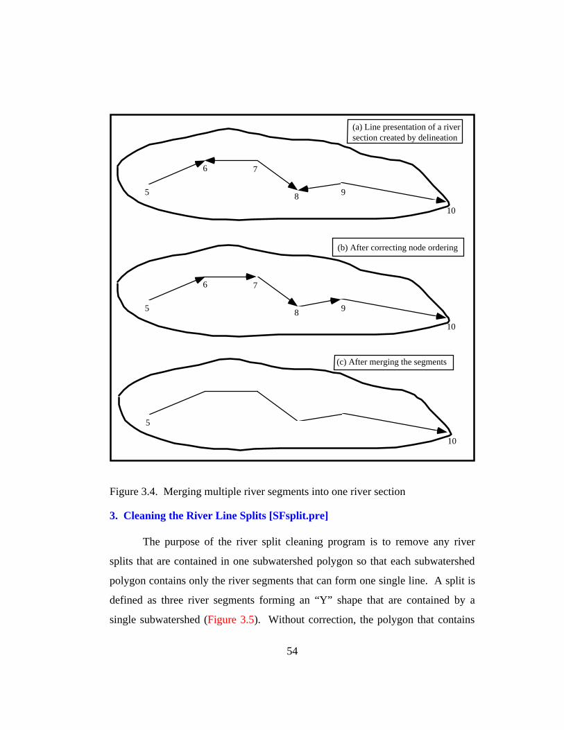
54
5
6 7
8 9
10
(a) Line presentation of a riversection created by delineation
5
10
5
6 7
8 9
10
(b) After correcting node ordering
(c) After merging the segments
Figure 3.4. Merging multiple river segments into one river section
3. Cleaning the River Line Splits [SFsplit.pre]
The purpose of the river split cleaning program is to remove any river
splits that are contained in one subwatershed polygon so that each subwatershed
polygon contains only the river segments that can form one single line. A split is
defined as three river segments forming an “Y” shape that are contained by a
single subwatershed (Figure 3.5). Without correction, the polygon that contains

55
split river lines will have a one-to-many relation with the river lines. The splits
are caused by the conversion procedure used transform a grid coverage to a vector
line coverage. When using the GRIDLINE or STREAMLINE functions to
convert a delineated grid lattice to a line coverage, the cells (referred to as joint-
cells) at the locations where three subwatersheds joint can assume any ID of these
three subwatersheds. If the ID-values assigned to the river line segments at the
joint cell are inconsistent with those assigned to the subwatersheds, the problem
of line split will occur. Although the lengths of these split lines are typically
small (1 to 1.414 times the grid cell size), each one of them still forms a record in
the spatial database file. Because of their small sizes, it is difficult to detect and
correct them manually.
The split-cleaning program works in the following way. For each polygon
in the river basin coverage, the program searches through features on the river line
coverage to select all the line segments that are contained within the polygon and
sends the selected lines to a list. If the number of line segments selected is greater
than one, then for each line segment in the list, the program saves its FNode
number. This FNode number is then used to select all the line segments in the list
that have that FNode as their TNode. If the number of selected lines is greater
than one, then an upstream split is found. To correct the problem, for each one of
the split segments, its FNode number is used to trace upstream to find its
upstream segment. Once an upstream segment is found, its stream ID is used to
reset the stream ID of the split river segment. Figure 3.5 illustrates the correction
of a split.

56
Polygon IPolygon II
Polygon III
ArcID=5
ArcID=5
ArcID=5ArcID=11
ArcID=13
(a) Before cleaning the splits
Polygon IPolygon II
Polygon III
ArcID=5
ArcID=13
ArcID=11ArcID=11
ArcID=13
(b) After cleaning the splits
RiverSections
BasinBoundaries
Figure 3.5. Rearranging river sections
3. Merging Multiple River Segments into one River Section [SFmg1ln.pre]
The purpose of the segment merging program is to merge any multiple
line segments contained by a single subwatershed polygon into one single line
object so that each subwatershed contains only one line section. To do this, the
program first creates a new line coverage (NewCov) from the old river line
coverage (OldCov). This NewCov is used to hold the river line objects that will
be merged. Then, for each polygon in the subwatershed coverage, the program

57
searches through the river line coverage (OldCov) to select the line segments that
are contained by the polygon. If the number of selected records equals one, the
program simply copies the river line object to the NewCov database. If the
number of lines selected is greater than one, the program will first check through
these lines to make sure they are connected to each other in a correct order from
upstream to downstream. If they are not, the program will correct the problem
based on the TNode and FNode indexes of each line segment. These line
segments are then merged and copied to NewCov. To merge these line segments,
the nodes and vertices of each line segment are extracted and put into a list based
on the order of the line segment. The merged line is then created from this point
list.
Upon the completion of the program, SFmg1ln.pre, the NewCov line
coverage, and the subwatershed polygon coverage have the following properties:
(1) each subwatershed polygon in the basin polygon coverage contains one and
only one river line section, (2) each river line section is contained by one and only
one subwatershed polygon, (3) the line sections are all connected in the order with
FNode on the upstream end and TNode on the downstream end, and (4) all the
vertices of a line are correctly indexed with the zero indexed node at the FNode.
Figure 3.4 shows an example result of applying SFsortr.pre and SFmg1ln.pre to a
river line coverage.
3.3. DATABASE DESIGN FOR SPATIALLY-REFERENCED TIME-SERIES DATA
Because the simulation model is constructed to simulate surface water
flow over both space and time, a database with a data structure that allows
efficient storage and retrieval of spatially-referenced time-series data needs to be
developed before the simulation model construction can start. This section

58
discusses the design of such a database and how spatially-referenced time-series
data are managed in this map-based surface water flow simulation model.
3.3.1. Two Types of Spatially-Referenced Data
Based on the number of values a physical parameter can have for one
location, spatially referenced physical data for a surface and ground water
simulation model can be divided into two categories, one value per location (or
one-to-one), and many values per location (or one-to-many). The examples of
one-to-one data type are: the area of a polygon, the latitude and longitude of a
point, or the length of a river section. Time-series data are of the one-to-many
data type. Examples include: precipitation records, runoff records, and water
level records.
During a modeling process, in order to store and retrieve these two types
of data efficiently, different data structures and retrieval methods need to be used.
In designing these data structures and data management systems, it is assumed
that a location feature, whether it is a polygon region, a line river, or a point
runoff station, can be uniquely identified by a location ID (COVER-ID).
3.3.2. Data Structure for Data of One-to-One Type
Data of the one-to-one type can be stored as location attributes attached to
a conventional GIS coverage. In this type of database, location ID is used as a
key field for data storage and it is also the only information needed to retrieve a
data value of a given physical parameter. The data structure of a one-to-one data
type is illustrated below in Figure 3.6.
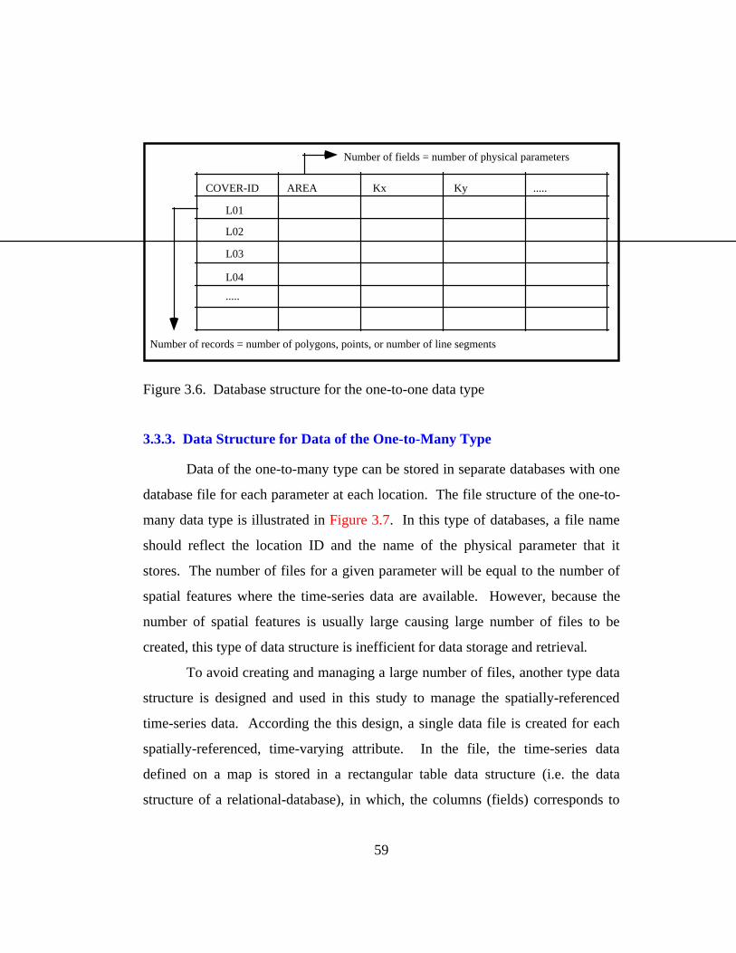
59
COVER-ID AREA Kx Ky .....
L01
L02
L03
L04
.....
Number of records = number of polygons, points, or number of line segments
Number of fields = number of physical parameters
Figure 3.6. Database structure for the one-to-one data type
3.3.3. Data Structure for Data of the One-to-Many Type
Data of the one-to-many type can be stored in separate databases with one
database file for each parameter at each location. The file structure of the one-to-
many data type is illustrated in Figure 3.7. In this type of databases, a file name
should reflect the location ID and the name of the physical parameter that it
stores. The number of files for a given parameter will be equal to the number of
spatial features where the time-series data are available. However, because the
number of spatial features is usually large causing large number of files to be
created, this type of data structure is inefficient for data storage and retrieval.
To avoid creating and managing a large number of files, another type data
structure is designed and used in this study to manage the spatially-referenced
time-series data. According the this design, a single data file is created for each
spatially-referenced, time-varying attribute. In the file, the time-series data
defined on a map is stored in a rectangular table data structure (i.e. the data
structure of a relational-database), in which, the columns (fields) corresponds to

60
the spatial features on a map and rows (records) corresponds to the time steps.
Figure 3.8 illustrates this type of data structure. The data structure is designed in
such a way that a one-to-one relationship exists between the fields of a time-series
database and the spatial features of the map on which the time-series data are
defined. The header (field name) is constructed by concatenating some letters
related to the name of the location with a unique location ID. The letters can be
the abbreviation of either the name of the attribute or the field name of the
location ID in the spatial database table.
The key field for this type of database is TIME for time-series data, and
STAGE-ID for multiple-stage data. To retrieve a data value for a given physical
parameter, one can first get the Location-ID from an appropriate map coverage,
then use the parameter name together with the location ID to open the appropriate
file and select the field associated with the location, and finally, use the STAGE-
ID or TIME value to locate the correct record for data retrieval.

61
Time/Stages
1
2
3
4
...
RUNOFF
RunoffL04
Time/Stages
1
2
3
4
...
RUNOFF
RunoffL03
Time/Stages
1
2
3
4
...
RUNOFF
RunoffL02
Time/Stages
1
2
3
4
...
RUNOFF
RunoffL01
(1) Number of files = Numbers of locations where time series records are available(2) FileName=Physical parameter name + location ID
Figure 3.7. The database files for the one-to-many data type
Number Of Fields = Number Of Records In (AAT/PAT)Field Names="GC"+ValuesOfCover_ID in (AAT/PAT)
Time/Stage GC1 GC2 GC3 ..........
1
2
........
Rec
ordN
umbe
r=T
imeS
teps
Figure 3.8. The database structure for one-to-many data type

62
3.3.4. Connections between Databases and the GIS Feature Attribute Tables
In ARC/INFO, feature attribute tables (FTAB) are INFO files associated
with each feature type. For a given coverage, a FTAB is created from a template
of standard items based on the feature types of the coverage. Figure 3.9 shows the
data structures for FTABs associated with each type of coverage.
As stated above, a single database with the template shown in Figure 3.6
can be created to store all the physical data of one-to-one type. The table is then
joined through a linking field (usually the COVER-ID) to the FTAB. Once this
table merge procedure is completed, the value of a given parameter at any location
can be retrieved using the value of the key field (COVER-ID). Because the data
items are merged with the value attribute table of a GIS coverage, data retrieval
and modification procedures are straightforward.
For the data of one-to-many type, a separate database table with the
template shown in Figure 3.8 is created. As this type of database is not
physically joined with the FTAB of a map, its data retrieval and modification at a
given location need are done through the linkage created by AVENUE programs.
To retrieve a time-series record, information about the parameter name, location
ID, and the TIME or STAGE-ID are needed. The parameter name and location
ID jointly tell the program which database file to open and which field to select,
and TIME allows the program to select the correct record number for data
retrieval. Figure 3.10 illustrates the data flow path for spatially-referenced time-
series data.

63
FND# TND# LPLY# RPLY# LENGTH COV# COVER-ID
Line coverage data attribute table structure (AAT)
Polygon/Point coverage data attribute table structure (PAT)
UserDefinedKeyField
UserDefinedKeyField
AREA PERIMETER COVER-# COVER-ID
Figure 3.9. Feature attribute tables in ARC/INFO
Shape Cover_ Cover_ID
** 1
2
3
4
Time GC1 GC2 GC3 GC4
Spatial Features (Map) Feature Attribute Table (PAT/AAT)
Table of Time-Series Data Sets
1
2
***
4
32
1
SomeFields
Figure 3.10. Connection between maps and spatially-referenced time-series data
3.4. CONSTRUCTION OF THE SURFACE FLOW SIMULATION PROGRAM
The map-based surface water flow simulation model simulates flow on the
river network based on the flow-routing equations introduced in Chapter Two and

64
the equations to be introduced in the following sections. In the model, water
movement in a river network is simulated at three levels: (a) watershed-to-river
water movement defined on a subwatershed polygon, which transfers either the
precipitation or the soil-moisture surplus into the local stream flow contribution,
PFlow(t), (b) water movement on a river section contained in a subwatershed
polygon, and (c) water movement between river sections on the river network
(inter-section water movements). The algorithm that simulates the water
movements between river sections also performs network analysis on the river
network to determine an appropriate sequence for simulating each subwatershed.
The algorithms that simulate water movements (a) and (b) are problem dependent
and are flexible. For this reason, this map-based surface water flow simulation
model can easily be modified to simulate other water flow related phenomena,
such as non-point source pollution analysis so long as the simulation module for
PFlow(t) is properly modified. The following sections show how water
movement is simulated in this map-based surface water flow simulation model.
3.4.1. Simulating Water Movement between River Sections
The following facts and concepts are used to construct the object-oriented
algorithm that simulates water movement on the river networks.
(1) A line coverage has been constructed using the method described in
Section 3.2.3. to represent the river network.
(2) A polygon coverage has been constructed using the method described
in Section 3.2.3. to represent subwatershed polygons.
(3) The features in the river line and subwatershed polygon coverages
have a one-to-one relationship so that the features of these two
coverages are connected through a common key field.

65
(4) Corresponding to each feature on the line and polygon coverages there
is a record in the river line attribute table (RFTAB) and polygon
feature attribute table (PFTAB) associated with their respective
coverages. Routing through the river network and subwatersheds
corresponds to processing though the records in the RFTAB, and
PFTAB.
(5) The water movement on the stream network is based on the principle
of continuity (e.g. Equations 3.1a and 3.1b) and the connectivity of the
network maintained by the From-Node and To-Node of each river line
object.
As shown in Tables 3.1 and 3.2 and in Figure 3.11, the PFlow (PFlow(t)
for unsteady state) associated with a subwatershed polygon object is used to
represent the object’s local flow contribution. FFlow and TFlow (FFlow(t) and
TFlow(t) for unsteady state) associated with a river line section are used to
represent the river flow rate at FNode and TNode of the river line object. Besides
applying the continuity equations (Equations 3.1 and 3.2) to the river network to
simulate the water movement between the river sections, this module also
determines a the order in which subwatersheds will be simulated.

66
(1)1
2
3
4
(2)
(3)FFlow3=TFlow1,3+TFlow2,3 - Rnode3
TFlow3,4=FFlow3*C3 + PFlow3
BasinBoundaries
RiverLines
FFlow1
FFlow3
••
•
•
PFlow3
TFlow3,4
Figure 3.11. River basin flow routing system
The sequential order is constructed using a stack-based algorithm. A stack
is an array (collection) that allows the Last-In-First-Out (LIFO) access to its
elements. The algorithm is described below (See Figures 3.12a and 3.12b).
When simulating the water movement between the river sections, each
stream line and each subwatershed are treated as entities. The effect that a stream
section and its subwatershed have on the stream network can be replaced by a
value, TFlow of the river section for steady state, or by a vector TFlow(t) for
unsteady state. In other words, as soon as TFlow, (or TFlow(t) for unsteady state)
of a subwatershed is acquired, the river section as well as the streams upstream of
the section can be cut-off from the remainder of the network.
As the algorithms used to simulate the physical processes in terms of
PFlow, FFlow, and TFlow depend on the modeling conditions and methodology
used, they can be different from one model to another. The flow simulation
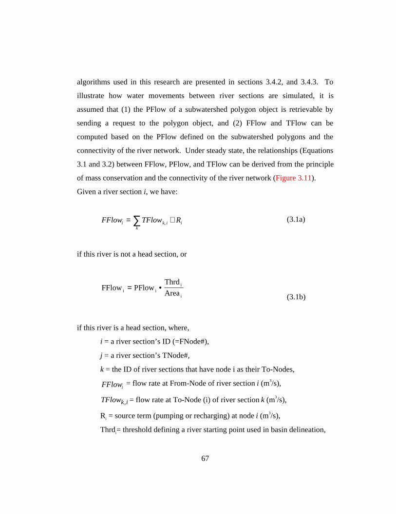
67
algorithms used in this research are presented in sections 3.4.2, and 3.4.3. To
illustrate how water movements between river sections are simulated, it is
assumed that (1) the PFlow of a subwatershed polygon object is retrievable by
sending a request to the polygon object, and (2) FFlow and TFlow can be
computed based on the PFlow defined on the subwatershed polygons and the
connectivity of the river network. Under steady state, the relationships (Equations
3.1 and 3.2) between FFlow, PFlow, and TFlow can be derived from the principle
of mass conservation and the connectivity of the river network (Figure 3.11).
Given a river section i, we have:
FFlowi = TFlowk, i + Rik
∑ (3.1a)
if this river is not a head section, or
FFlow PFlowThrd
Areai ii
i
= •(3.1b)
if this river is a head section, where,
i = a river section’s ID (=FNode#),
j = a river section’s TNode#,
k = the ID of river sections that have node i as their To-Nodes,
FFlowi = flow rate at From-Node of river section i (m3/s),
TFlowk,i = flow rate at To-Node (i) of river section k (m3/s),
Ri = source term (pumping or recharging) at node i (m3/s),
Thrdi= threshold defining a river starting point used in basin delineation,

68
Areai= area of the subwatershed that contains river section i (m2).
The flow rate at the To-Node is given by:
TFlowi , j = FFlowi * Ci + PFlowi − DFlowi(3.2a)
if this river line is not a head section, and
TFlow PFlow DFlowi j i i, = −(3.2b)
if this river line is a head section, where,
i = river section ID,
Ci = river sectional flow gain/loss coefficient of river section i (1/m),
PFlowi = runoff contribution of river basin polygon i, that contains river
section i (m3/s),
DFlowi = flow diversion on river section i (m3/s).
Figures 3.12a and 3.12b show the program flow chart of the module that
simulates the water movement between river sections. The center-piece of the
algorithm is a stack used to keep track of the stream lines that the model has
traveled, so the algorithm can be called a stack-based stream network analysis
algorithm. The logic of the algorithm is explained below.
It can be seen from the program flow chart (Figures 3.12a and 3.12b) that,
for a given river section, the program starts with searching upstream to find the
stream sections flowing into it. There are three possible outcomes of the search.
(1) If no upstream section is found, and the section is not the head section,
then a mistake must have occurred either in the programming procedure or in the

69
stream network formulation. The program will exit and print an error message for
program debugging.
(2) If one or more upstream sections are found, at least one of them is not
yet simulated, the current river object (identified by its ID) is pushed into the
stack and the program moves upstream to one of the river objects not yet
simulated. This procedure is repeated until a head section is found. Once a head
section is identified, the program searches through the subwatershed polygon
attribute table (PFTAB) to identify the subwatershed containing the head section.
If none is found, the program exits and prints an error message. Otherwise, the
program issues a request to the flow simulation module defined on the
subwatershed polygon to get PFlow. Equations 3.1b, and 3.2 are used to compute
the FFlow and TFlow of the river object. Once this is done, the algorithm moves
to the next downstream river section by issuing a pop request to the stack. At this
downstream section, the algorithm again searches upstream and checks the if all
the upstream sections have been simulated. Based on the outcome of this search
and test, the program decides if it can simulate water movement on the current
river object or whether it must push this stream object into the stack and move
upstream.
(3) If one, or more than one upstream sections are found, and all have
their flow simulations completed (indicated by state value, isdone=1), the river
flow is simulated at the current section. The program searches for the
subwatershed containing the current river section. One and only one basin should
be found. If not, the program prints out an error message and exits. Otherwise,
the program issues a request to the subwatershed polygon to get the PFlow and
uses Equations 3.1a and 3.2 to compute FFlow and TFlow.

70
The procedure is repeated until the outlet section is reached and its flow is
simulated. This procedure is illustrated in the flowchart shown in Figures 3.12a
and 3.12b.
The program is designed in such a way that it allows the model to be
applied on any user defined portion of a river basin. The program can also be
used to simulate water flow in a region having more than one river network.

71
Program Starts:(1) Initilize computation related attributes(2) Select a stream to start the computaton(3) Create a stack (RvSt) to hold river id (rvid)
Yes
AllDone=0 LFound=0
No
No
Yes
No
Error: Exit level(1)
Yes
Loop 2: basin polygon objects
Loop 1: river line objects
PFound=0
NoError: Exit level(2)
YesError: Exit level(3)
Yes
No
Send request to getPFlow(t) from thepolygon flow model
Yes
Model run completesExit level(0)
rvid=rvst.popStart movingDownstream
Update FFlow ofdownstream riversection (rvid)
Send a request to a rivermodule to get TFlow(t)
Update: TflowLisdone=1
RvSt.Push(rvid)Move upstream
No
If((isOutlet) or(RvSt.IsEmpty))
If(AllDone)
IsHead(rvid)
If(PFound)
If(PisDone)
If(LFound)
Update: PFlowPisDone=1
Figure 3.12a. The main loop of algorithm simulating water movement within andbetween subwatersheds

72
Get LTnodeV Get IsHeadVGet IsDoneV Get IsOutletV
NoYes
YesNo
AllDone=1
LFound=1
Given FnodeC
IF(TnodeV=FnodeC)
IF(IsDoneV=1)
IsLastStream
AllDone=0, EXIT
EXIT
Next Stream
Loop ONE:Loop throughstream class insearching forthe upstreamriver section
Get the first stream
Get PGCodeVGet IsDoneV
PFound=1EXIT
NextBasin
Given A LGCodeV Get a basin polygon
PGCodeV=LGCodeVIsLastBasinNo Yes
PFound=0EXIT Yes
No
Loop TWO:Given LGCodeVsearching fora basin poly withPGCodeV=LGCodeV
Figure 3.12b. Subloops of the algorithm simulating water-movement within andbetween subwatersheds

73
As an example to show how inter-subwatershed water movement is
simulated on a river network, line section 25 (be referred to as S25 here after) in
Figure 3.13 is selected to start a simulation run. The sequence by which the
simulation model is applied to each river section on the stream network is
described below.
From S25, realizing its upstream section S27 has not been computed yet,
the program pushes S25 into the stack and moves upstream to S27. Because S27
is a head section, the program gets PFlow from the subwatershed containing S27,
computes FFlow and TFlow for S27, then issues a pop request to the stack to get
S25 and moves downstream to S25. On S25, it finds that S33, another upstream
section of S25, has not been simulated. The program again pushes S25 into the
stack and moves upstream to S33, gets the PFlow from the polygon containing
S33, and moves downstream to S25. This time, the program finds that all its
upstream sections (S27, S23) have been simulated and it is time to simulate water
movement from the From-Node to To-Node of S25. The model will then activate
a module that simulates water movement between the From-Node and To-Node of
a river section to simulate the water movement on section S25. After this, the
program sends a pop request to the stack to get S18 and moves downstream to
S18. This procedure is repeated until the outlet section is reached and simulated.
Figure 3.14 gives the sequence by which the program visits and simulates river
sections on the river network shown in Figure 3.13.

74
Figure 3.13. The Guadalupe River Basin
* S25 S27 S25 S33 S25 S18 S21
S35 S28 S40 S39 S40 OutletReached (Loop 14 times )
S18
S28
Figure 3.14. Program travel path given by the stack-based algorithm
3.4.2. Simulating Water Movement within a River Section
This section describes how water movement from the From-Node to the
To-Node on a river section is simulated. As discussed at the beginning of this
section, this simulation model is designed in such a way that by changing the
modules used to compute PFlow, FFlow, and TFlow (element functions), the
model can be used to simulate different hydrologic processes without changing
the stack-based stream network analysis procedure.
In this map-based surface water flow simulation model, four flow routing
modules are available to simulate water movement between the From-Node and
the To-Node. These four modules use (1) a response function method, (2) a two-
step function method, (3) dam/reservoir model combined with the two-step
function method, and (4) a Muskingum-Cunge method. All of these four modules

75
are constructed based on the principle of continuity. Figure 3.15 shows the logic
of the program used for river routing. IMax in Figure 3.15 stands for the
maximum time step interval allowed before the Muskingum method becomes
unstable. HasDam, HasResp, and Muskingum are the states of a river line object
given in Table 3.2. As can be seen from this figure, the decision of selecting one
specific simulation module (out of four) is made based on the river features at run-
time. The theory and programming methodology used to construct each of these
four modules are discussed below:
.
Given a river section HasDamYes
Call D
amR
outingProgram
No
HasRespYes
Get Resp. function &compute TFlow(t)using Eq 3.3
Muskingum
No
NoYes
Istep< IMax
No
Yes
UseMuskingummethod for theriver routing
Use the Two-Stepflow routingprocedure tocompute TFlow(t)
START
END
END
Figure 3.15. Program flow chart of river section flow routing module
(1) The Response Function-Based Flow Routing Module
The state, HasResp, of a river line object, indicates if a user-supplied
response function (Maidment, 1993) is available for the river section. HasResp=0
indicates no response function is available and HasResp=k (k≠0) indicates a user-
supplied response function is available and the response function has k

76
components. When a river section has a response function that takes the water
flow time-series at the From-Node as an input and produces the flow time-series
at the To-Node as an outputs, this response function is used to simulate water
movement between the From-Node and To-Node of the river section. The
response-function-based flow routing module is constructed using the following
equation:
TFlowi, jt = FFlowi
t −k
k=0
min(t,N )∑ ⋅Ui
k + PFlowit − DFlowi
t − Lossit (3.3)
where,
TFlowi, jt = TFlow of river section i (with j as its To-Node), at time step t
(m3/s),
FFlowit −k = FFlow of river section i at time step t-k (m3/s),
Uik = the response function of N elements for river section i,
PFlowit = PFlow of subwatershed i at time step t (m3/s),
DFlowit= flow diversion of river section i at time step t (m3/s),
Lossit = stream water loss of river section i at time step t (m3/s).
The water loss in a river section is computed using the following equation:
Lossit = FFlowi
t ⋅ Lengthi ⋅ LossCi (3.4)
where, Lengthi = the length of river section i, (m),
LossCi = loss coefficient of river section i, (1/m), a river line attribute that
can be used as a model calibration parameter.

77
(2) The Two-Step Flow Routing Module
This flow routing model is a special case of the response function flow
routing model. This module is used when a user-supplied response function is not
available and when the use of Muskingum method is not computationally
efficient, i.e., when the size of simulation model time step is much greater than
the average travel time through the reach, ∆t >>Li
vi
. Given below is the equation
used for the two-step flow routing module:
TFlowi , jt = FFlowi
t −1 ⋅ Llagi + FFlowit ⋅(1 − Llagi )
+ PFlowit − DFlowi
t − Lossit
(3.5)
where, Llagi = The normalized time lag between From-Node and To-Node
of river section i,
Llagi =Li
Vi
∆t, (3.6)
Li = the length of river section i (m),
Vi = the average flow velocity on river section i (m/s),
∆t = the size of simulation time step.
As it can be seen from Equation 3.5, the two-step flow routing module is
based on the principle of continuity of water flow and guarantees that the water
mass will be preserved.

78
(3) Dam and the Two-Step Flow Routing Module
The state, HasDam, of a river line object, indicates if dams (or reservoirs)
exist on the river section. HasDam=0 indicates there is no dam on the river
section. HasDam=k, (k≠0) indicates there is at least one dam located on the river
section, and the value k is also the ID number of the first dam on the section.
When one or more dams exist on a river section, the reservoir routing procedure
(DAMRT.ave) is called to simulated the effects of reservoirs on the river flow.
Whenever reservoirs exist on a river section, the two-step flow routing module is
used to simulate the water movement on the river segments between the dams and
From-Node and To-Node of the river section. The dam simulation module is
discussed in Section 3.5.1.
(4) Muskingum-Cunge Flow Routing Module
The state, Muskingum, of a river line object, indicates if the Muskingum-
Cunge river routing method will be used for the river section. Muskingum=0
indicates the Muskingum method will not be used to simulate water movement on
the river section and Muskingum=n (n≠0) indicates that the Muskingum flow
routing method will be used if the number of internal loops is less than n. The
internal loops are constructed to ensure the computational stability of the
Muskingum river flow routing procedure. The internal loop is discussed further
below. The Muskingum-Cunge method is introduced in Chapter Two and the
flow routing equations derived for the method are reproduced here as Equations
3.7 and 3.8.
TFlow C FFlow C FFlow C TFlow Ci jt
it
it
i jt
, ,= ⋅ + ⋅ + ⋅ +− −1 2
13
14 (3.7)

79
where,
C1 =∆t − 2KX
2K(1 − X) + ∆t(3.8a)
C2 =∆t + 2KX
2K(1− X ) + ∆t(3.8b)
C3 =2K(1 − X) − ∆t
2K(1 − X) + ∆t(3.8c)
C4 =PFlowi
t − DFlowit − Lossi
t
2K(1 − X) + ∆t, (3.8d)
Kx
c=
∆, K is a storage constant [T], (3.8e)
X =1
2−
Avg(TFlow, FFlow)
2c B Se∆X (3.8f)
X = a weighting factor showing the relative importance that FFlow and
TFlow have on a river section’s storage, (0 ≤ X ≤ 0.5) , where 0
indicates pure storage and 0.5, indicates pure translation,
c = kinematic wave velocity (m/s),
B = cross-sectional top width associated with average of TFlow and
FFlow,
Se = the energy slope,
∆x = the length of a river section.
To ensure the stability of the flow routing, C3 needs to be greater than
zero. From equation 3.7c, it can be seen that in order for C3 ≥ 0 , we need to have
∆t ≤ 2K(1− X) . When the simulation time step ∆t does not satisfy this
relationship, the time step needs to be subdivided into smaller steps. In the
simulation model, C3 ≥ 0 is achieved by subdividing a simulation model time

80
step into multiple n internal time steps so that ∆ti =∆t
n≤ 2K(1− X ) . When n is
too large, the round-off errors accumulated by the internal loop may outweigh the
benefits brought by using the Muskingum-Cunge method. In this event, the
simulation model switches to use the two-step function flow routing module
(Figure 3.15).
3.4.3. Simulating Water Movement within a Subwatershed
In this map-based surface water flow simulation model, PFlow(t)
represents local runoff generated in a subwatershed. Several methods are
available to calculate PFlow(t) from precipitation observations, e.g. by spatially
interpolating the precipitation to the center point of each subwatershed and then
converting the precipitation to PFlow(t). In the Niger River Basin simulation
model, PFlow(t) is constructed from the soil-moisture surplus time-series
produced using a simple bucket model. As the input data sets for the soil-
moisture balance model, monthly time-series tables of precipitation and potential
evaporation for the period July 1983 to December 1990 were estimated at each
point on a regular mesh of 0.5 degree cells covering the study area. This
computational mesh was selected because long term mean monthly estimates of
rainfall and temperature at these points were available from C.J. Willmott at the
University of Delaware. As discussed in Chapter Two, a convolution procedure
(Olivera and Maidment, 1996) is used to convert soil-moisture surplus to local
runoff (SurpF(t)-> PFlow(t)).
Using this method, PFlow(t) is simulated with two flow components. One
is SFlow(t) used to simulate the overland flow and the other one is OFlow(t) used
to simulate the subsurface water flow. The overland flow is estimated by
applying the concept of unit hydrograph to the soil surplus, SurpF(t). The
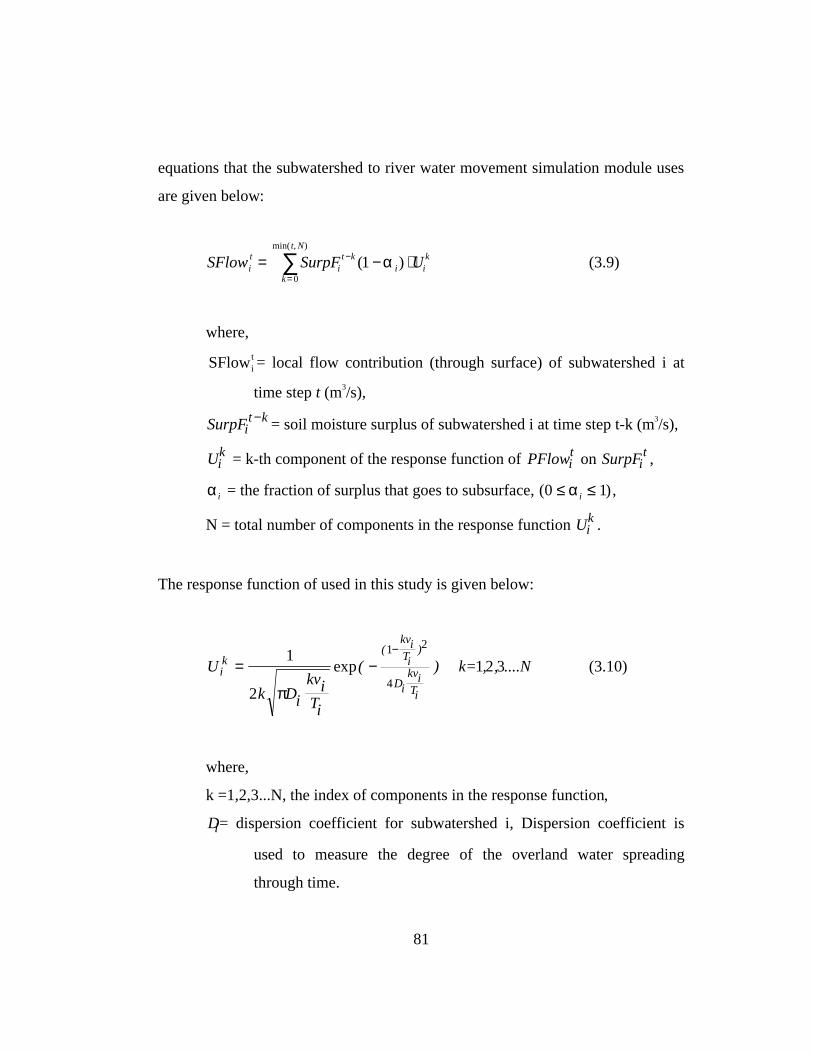
81
equations that the subwatershed to river water movement simulation module uses
are given below:
SFlowit = SurpFi
t −k
k= 0
min( t, N)
∑ (1 −α i) ⋅Uik (3.9)
where,
SFlowit = local flow contribution (through surface) of subwatershed i at
time step t (m3/s),
SurpFit −k = soil moisture surplus of subwatershed i at time step t-k (m3/s),
Uik = k-th component of the response function of PFlowi
t on SurpFit ,
αi = the fraction of surplus that goes to subsurface, (0 ≤ αi ≤ 1),
N = total number of components in the response function Uik .
The response function of used in this study is given below:
U
k DikviTi
( ) k= , , ....Nik
(kviTi
)
DikviTi
= −−1
2
1 2 31 2
4π
exp (3.10)
where,
k =1,2,3...N, the index of components in the response function,
Di= dispersion coefficient for subwatershed i, Dispersion coefficient is
used to measure the degree of the overland water spreading
through time.

82
Vi = average overland flow velocity for subwatershed i, (m/s),
Ti = average overland flow time for subwatershed i (s).
The values of these parameters for a subwatershed can be estimated either
through hydrologic analysis of the subwatershed or through the optimization
module to be discussed later in this chapter.
The subsurface water flow component of PFlow(t) is considered to be
going through an imaginary underground reservoir. The flow through the
reservoir can be simulated using a linear reservoir model. Equations used to
perform flow routing through a linear reservoir are given below:
OFlowit = Si
t −1 / Ki (t = 1,2,3,....) (3.11)
Sit = Si
t −1 + (SurpFit ⋅ αi −OFlowi
t ) ⋅ ∆t (3.12)
where,
OFlowit = the subsurface flow component at time step t, on polygon i
(m3/s)
Sit = storage of the under-ground-reservoir at time step t, on polygon i
(m3),
Ki = the linear reservoir constant representing the average residence time
of water in the reservoir (s).
After these two components are computed, the local flow contribution of
subwatershed i at time step t is computed using Equation 3.13.
PFlow SFlow OFlowit
it
it= + (3.13)

83
3.5. OTHER SIMULATION MODEL OBJECTS
This section describes three other classes of objects used in the simulation
model, dam/reservoir object, flow-check object, and flow-diversion object. All
these objects appear as a points on a point coverage and are located on a river line
object. The point location on the river line is dynamically calculated from a user
specified cursor location. The algorithm that performs the dynamic line
segmentation is described in Section 3.6.4.
3.5.1. The Dam Objects
The dam/reservoir objects are designed to simulate the effects of dams and
reservoirs on river flows. The states of a dam/reservoir object are given in Table
3.3. A utility program is available to construct dam/reservoir object directly and
interactively from a river map. For each dam object created, a new record is
added to the dam feature attribute table (FTAB) and a time-series table is created
to hold time-series data sets for reservoir routing. The states of a dam object are
listed in Table 3.3a and the fields in the dam routing time-series table are given in
Table 3.3b. The graphic point on the dam coverage is connected to the dam’s
FTAB through the shape field in the FTAB. The connection to its associated
time-series table is established through the DamId and the name of the time-series
table.
During a flow simulation, the presence of a dam/reservoir object is
detected by the simulation model through the return value of the HasDam state of
a river section.
HasDam=0 indicates that no dam is located on the river section. The
return of a non-zero value of HasDam indicates that there is at least one dam on

84
the river section and the non-zero value is the Dam-ID of the first dam located on
the river section.
Table 3.3a. The Attributes of a Dam/Reservoir Object
State Function (What the attribute represents)Shape Pointer pointing to the map location of the objectDamid The ID of a dam/reservoir object, Damid is also a pointer pointing to the time-series
table associated with the reservoirDamName The name of a dam/reservoirCapacity Capacity of a reservoir (m3)Area The water surface area of the reservoir when storage=capacity (m2)Upst The active storage of the dam/reservoir (m3)DeadSt The dead storage of the dam/reservoir(m3)Evt The evaporation rate of the reservoir (mm/day)Pdam Damid of the upstream dam located on the same section, 0=No upstream damNdam Damid of the dam downstream of the dam on the same stream section, 0=No dam
located downstreamStorage0 Initial storage of the reservoir (m3)Area0 Initial water surface area of the reservoir (m2)
Table 3.3b. The Fields of a Dam-Routing Time-Series Table
FieldName Function (What the attribute represents)Time Simulation time stepsInflow Inflow time-series of the reservoir (m3/s)DmdFact Demand factor of each simulation time stepWithDraw Water withdraw of each time stepNetEvp Net evaporation of each time step (mm/day)Sarea Surface area of each simulation time step (m2/s)Spill Discharge (including water used for power generation) of each time step (m3/s)Storage Storage at the end of each simulation time step (m3/s)
In the process of a river flow routing, if a reservoir is detected on a river
section, the river routing program will call the dam simulation module DAMRT
and pass the Dam-ID and FFlow(t) to DAMRT. The DAMRT module will then
simulate the behavior of the reservoir. The simulation is based on the information
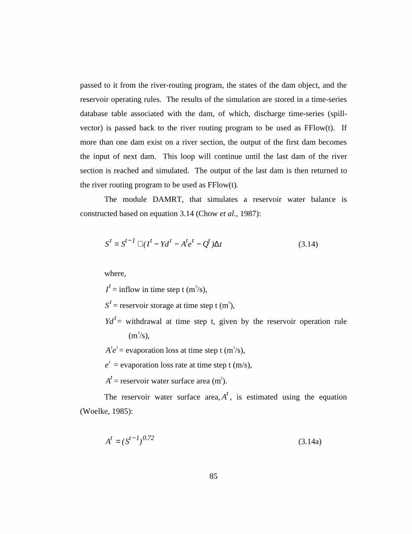
85
passed to it from the river-routing program, the states of the dam object, and the
reservoir operating rules. The results of the simulation are stored in a time-series
database table associated with the dam, of which, discharge time-series (spill-
vector) is passed back to the river routing program to be used as FFlow(t). If
more than one dam exist on a river section, the output of the first dam becomes
the input of next dam. This loop will continue until the last dam of the river
section is reached and simulated. The output of the last dam is then returned to
the river routing program to be used as FFlow(t).
The module DAMRT, that simulates a reservoir water balance is
constructed based on equation 3.14 (Chow et al., 1987):
St = St −1 + (I t − Yd t − Atet − Qt )∆t (3.14)
where,
It = inflow in time step t (m3/s),
St = reservoir storage at time step t (m3),
Yd t= withdrawal at time step t, given by the reservoir operation rule
(m3/s),
Atet = evaporation loss at time step t (m3/s),
et = evaporation loss rate at time step t (m/s),
At = reservoir water surface area (m2).
The reservoir water surface area, At , is estimated using the equation
(Woelke, 1985):
At = (St −1)0.72 (3.14a)

86
where, Qt = reservoir water release to downstream at time step t (m3/s).
Reservoir release is given by the reservoir’s operating rule subject to the
following constraints:
Qt ≥St −1
∆t+ (I t − Ydt − Atet ) −
Sc
∆t(3.15a)
Qt ≤St −1
∆t+ (I t − Ydt − Atet) −
Sd
∆t(3.15b)
where, Sc = the reservoir storage capacity (m3),
Sd = the reservoir dead storage (m3).
Relation 3.15a ensures that at any time step, the reservoir storage will not
be greater than the reservoir capacity, and relation 3.15b ensures none of the water
in the dead storage goes into release.
Inflow to a reservoir is computed differently based on the location of the
reservoir. When a reservoir is located at a non-head river section and is the first
on the river section, Equation 3.16a is used to compute the inflow.
I t = FFlowt(1 − Llag) + FFlowt −1 ⋅ Llag + PFlowt ⋅∆A
A(3.16a)
where,
Llag =(XL / v)
∆t = fractional time it takes for water to travel from the
From-Node to the location of the dam,
XL = the distance between the From-Node and dam location (m),

87
v = river flow velocity (m/s),
∆t = the size of time step of the simulation (s),
∆A = regional area between FNode and the reservoir location (m2).
When∆A is not given, it can be estimated using Equation 3.16b:
∆A =XL
TL⋅ A (3.16b)
A = the total area of the subwatershed where the reservoir is located,
TL = total length of the river section.
When a reservoir is located at a head section and is the first on the river section,
Equation 3.16c is used to compute the inflow.
[ ]I PFlow Llag PFlow LlagA
A
PFlowA
A
t t t thrd
t
= ⋅ − + ⋅ ⋅
+ ⋅
−( ) ( )1 1 ∆
∆
(3.16c)
where, ∆Athrd = threshold area that initializes a river used in watershed
delineation procedure.
Comparing Equation 3.16c with 3.16a, it can be seen that in the head river
section, FFlowt = PFlowt ⋅(∆Athrd
A) . When a reservoir is not the first reservoir
on a river section, its inflow is computed using equation 3.16d.

88
Iit = Qi −1
t ⋅(1 − Llag) + Qi −1t −1 ⋅ Llag[ ]+ PFlowt ⋅
∆A
A(3.16d)
where,
i = sequential numerical index of the dams in a river section with i=1 for
the first dam on the river section. i=2,3,4..,
Llag =(XL / v)
∆tthe fractional time it takes for water to travel from dam i-1
to i,
XL = travel distance along the river line from dam i-1 to i,
Qi−1t = water release of reservoir i-1 at time step t. (m3/s).
It can be seen from the equations above that dam simulation module uses
Equations 3.14 and 3.15 to perform the reservoir water balance computation and
uses the two-step flow routing module to simulate the flow in the river segments
between the dams. More complex reservoir operating rules such as the ones
introduced in the works of Loucks (Loucks, 1981) could also be included in this
dam/reservoir simulation model.
3.5.2. The Flow-Check Point Objects
The flow-check objects are created at the locations where stream flow
estimations are desired because the simulation model produces the flow estimates
only at the From-Node and To-Node of each river section. A utility program is
written to allow the interactive construction of these objects on a river network.
Table 3.4 lists the attributes of a flow-check point object. The algorithm used to
interpolate flow rate to a flow-check point is discussed in Section 3.6.4.

89
Table 3.4. Attributes of a Flow-Check Point Object
State Function (What the attribute represents)Shape Pointer pointing to the map location of the objectPointid Identification number of a flow-check pointFFlow FFlow of the river line object on which a flow-check point is locatedTFlow TFlow of the river line object that a flow-check point is locatedIFlow Flow interpolated at a flow-check pointOline A flag specifying if a flow-check point is located on a river (Oline=0 indicates the
flowchk point is on the river line, Oline=1 indicates the point is not on the river linebut within the simulated area, and Oline=-1 indicates the point is out of the area)
Pcntage between the distance of a Flow-Check point to From-Node and the length of theriver section.
Length The length of the river section where a flow-check point is located
3.5.3. The Flow-Diversion Point Objects
When a flow diversion point has a constant flow rate, it is incorporated
into the river object associated with the point. The diversion rate is put into the
attribute DFlow of a river object. When a flow diversion point has a time-varying
flow rate, it can be simulated using the reservoir object with constant storage and
no evaporation loss. These objects are detected and simulated by the river flow
routing module.
3.6. UTILITY PROGRAMS AND POST-PROCESSORS
The utility programs of this map-based simulation model are constructed
to allow interactive model modification and make easy result presentations
possible. This section describes the designs of these interactive model
modification and result presentation programs.

90
3.6.1. Construction of a Sub-Model
When simulating surface water flow process on a large river basin, it is
sometimes necessary to isolate a portion of the river basin for more detailed study.
For this purpose, it is desirable to clip a portion of the river basin from the main
model to form a sub-model. When a simulation model is constructed in the
traditional means, constructing such a sub-model requires an effort comparable to
that used to construct the original basin model. In this map-based simulation
model, however, a sub-model can be constructed interactively from the existing
basin model in a ’real-time’ operating style, i.e. when a portion of the map is
selected and copied, a new model of the selected region is created. The procedure
to create a sub-model is listed below:
(1) select the maps necessary to create the model by making their
corresponding themes active in an ArcView’s view window,
(2) select the features (polygons, lines, or points) from each map that fall
into the study region of the sub-model,
(3) run the sub-model construction utility program (CLIPMDL.utl) to
create the sub-model.
Because the model is constructed based on the concept of object-oriented
programming, the newly created sub-model inherits all the features of the original
model. Therefore, once constructed, all the programs applied to the original
model can be applied to the sub-model. Figure 3.17 in Section 3.6.2 shows an
example of a sub-model. The logic of the program that enables interactive sub-
model creation is explained below.
It is known that for each feature object on a geographic map there is a
record in the relational database table containing the states of the object and the
model programs have the ability to access both the map feature and its associated

91
record. In procedure (1), at the same time when each map is selected, its related
database table is also selected, and in procedure (2), when features on these maps
are selected, their corresponding records in the database tables are also selected.
The functions of the sub-model construction program [CLIPMDL.utl] are
(1) to make one copy of map-templates (class) for each user-selected map, (2) to
loop through each selected database table and copy the selected records to its
newly created map-template, and (3) to create an alias for the newly-created maps
so that they are the same as those for the maps in the original models. The reason
that newly created maps keep the same alias as those of its original maps is that
the maps are referenced in the model programs by their alias. Programs identify
maps by their alias rather than their real file name, and if the maps of the sub-
model have the same alias as those of original maps, all the programs used in the
original model can be applied to the sub-model without any modifications.
The sub-model construction utility program also identifies the sources of
the river network so that inputs related to those streams can either be inherited
from the original model simulation results or supplied by the user. A source
stream is defined as a river section whose inflow streams in the original model are
cut off by the clipping procedure.
3.6.2. Optimization Algorithms
This section describes the optimization algorithms developed for the
purpose of simulation model calibration. Two optimization algorithms, multi-
directional and interactive, are developed in this research for the purpose of model
calibration. Both algorithms require a user to provide, on a space defined by the
optimization variables, a value range for each variable to be calibrated. The
interactive model usually requires multiple runs to get an optimal solution and for
each optimization process, a new solution space based on previous runs needs to

92
be defined. The second method, multiple directional optimization requires a user
to define only the solution space at the beginning of a calibration process. After
the solution space is defined, the optimization model applies a bisection algorithm
on each dimension to search for an optimal solution set. The concepts of both
optimization modules are discussed below in Sections 3.6.2.1. and 3.6.2.2.
3.6.2.1. The Interactive Optimization Algorithm
The purpose of this interactive optimization algorithm (IOA) is to calibrate
the model parameters for this map-based simulation model. The optimized
parameters are defined as a set of parameters that produce a best-fit between a
simulated and observed river flow time-series at a given location. Two standards
(match standard) used by the algorithm to evaluate the extent of fit are: sum of
mass discrepancies (SMD) and sum of root mean square errors (RMSE). A best-
fit time-series can be defined as the time-series that minimizes RMSE and
produces zero SMD. SMD function is used to ensure that the average flow rate
produced by the simulation model equals that of the observed in the same period
of time. RMSE function is used to pursue the best match between the simulated
flow time-series and observed flow time-series. Since the model is designed in
such a way that the optimization algorithm is independent of the match standards
used, a user of the model can add other standards to achieve better matches on the
low flow and peak flow period. Mathematically, the sum of mass discrepancies
can expressed as:
SMD =(Ot − Ft)
t =1
n
∑Ot
t =1
n
∑(3.17)

93
The sum of root mean square error can be expressed as:
RMSE
O F
O
t t
t
n
t
t
n=−
=
=
∑
∑
( )2
1
1
(3.18)
where, Ot = observed flow rate at time step t at a flow gage station,
Ft = simulated flow rate at time step t at the same flow gage
station. The function Ft can be written as:
Ft = F(x1,x2, x3,...xn ) (3.19)
where, x1,x2, x3,...xn = model parameters. The parameter optimization
problem becomes the problem of finding a parameter set
r P = x1, x2 , x3, ...xn{ } that
satisfies:
SMD =(Ot − Ft)
t =1
n
∑Ot
t =1
n
∑= SMD(x1, x2 , x3, ...xn ) = 0 (3.17a)
and minimizes:

94
RMSE
O F
O
x x x x
t t
t
n
t
t
n n=−
=
=
∑
∑ = RMSE
( )
( , , ,... )
2
1
1
1 2 3 (3.18a)
As an example to show how the interactive optimization algorithm works,
the procedure of optimizing two variables, X1 and X2, for a simulation model
based on the standards imposed in Equations 3.17 and 3.18 is described below.
The algorithm assumes that the lower and upper limits of X1 and X2 are
known or could be reasonably estimated. Let the lower and upper limit for X1 and
X2 be designated as x1min, x1max, x2min, and x2max, respectively. The optimization
problem is equivalent to finding the X1, X2 combination from the parameter space
{X1,X2} that gives a minimum SMD and RMSE (Figure 3.16). The algorithm
first discretizes each variable (represented as one dimension in the parameter
space) into a user specified range. In this example, 6 steps are specified for
parameter X1 and 5 for X2. As a result, 30 X1~X2 parameter combinations are
formed. The interactive optimization algorithm then uses these parameter sets to
run the simulation model 30 times, and computes the RMSE and SMD based on
each simulation result. The parameter set that returns the minimum RMSE or
SMD is manually selected as the first estimate. A finer step size can now be used
to form another grid around the first estimate to form another parameter set in
search for a better fit. The procedure can be repeated several times until an
optimal is found.
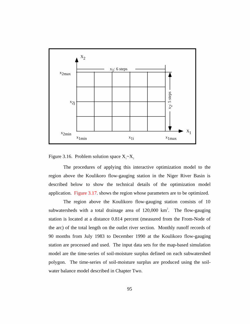
95
.
X2
X1
x2max
x2minx1min x1maxx1i
x2j
x1: 6 steps
x 2: 5
ste
ps
Figure 3.16. Problem solution space X1~X2
The procedures of applying this interactive optimization model to the
region above the Koulikoro flow-gauging station in the Niger River Basin is
described below to show the technical details of the optimization model
application. Figure 3.17. shows the region whose parameters are to be optimized.
The region above the Koulikoro flow-gauging station consists of 10
subwatersheds with a total drainage area of 120,000 km2. The flow-gauging
station is located at a distance 0.814 percent (measured from the From-Node of
the arc) of the total length on the outlet river section. Monthly runoff records of
90 months from July 1983 to December 1990 at the Koulikoro flow-gauging
station are processed and used. The input data sets for the map-based simulation
model are the time-series of soil-moisture surplus defined on each subwatershed
polygon. The time-series of soil-moisture surplus are produced using the soil-
water balance model described in Chapter Two.
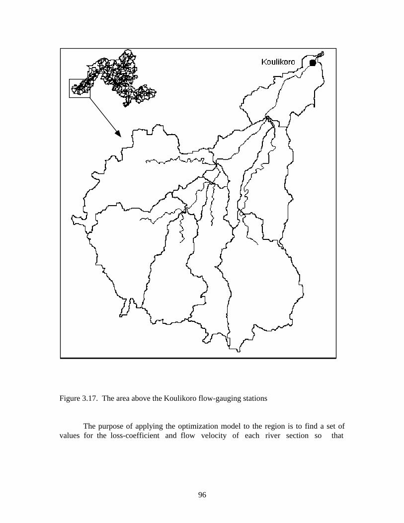
96
Figure 3.17. The area above the Koulikoro flow-gauging stations
The purpose of applying the optimization model to the region is to find a set ofvalues for the loss-coefficient and flow velocity of each river section so that

97
the river flow time-series produced by the simulation model at Koulikoro matches
that of observed at the location. The match is defined by Equations 3.17 and 3.18.
As an estimate, ranges of the loss-coefficient1 and average flow velocity
on the river are estimated as below:
0.00001 ≤ lossC ≤ 0.0007 (1/km)
0.2 ≤ V ≤ 0.55 (m/s) (3.19)
The range of each variable is divided into 4 intervals with 5 steps, which
creates a testing space of 5x5=25 data sets. After applying the interactive
optimization model under such conditions, four charts are generated by the model
to show the parameter values that produce the best fit. These four charts are (1)
RMSE vs. parameter set (Figure 18a), (2) SMD vs. parameter set (Figure 18b), (3)
flow time-series plot of observed vs. simulated when RMSE is the minimum, and
flow time-series plot of observed vs. simulated when |SMD| is the minimum. The
last two charts are not shown here because similar charts will be produced later in
Section 3.6.2.2.
Figures 3.18a and 3.18b show the plots of SMD and RMSE for each
parameter sets. It can be seen from the plots that the minimum RMSE can be
achieved by adjusting the river velocity while the minimum SMD can be achieved
by adjusting the loss-coefficient of the river. In most situations, to have zero mass
discrepancy between the simulated time-series and the observed time-series is
very important. Figure 3.18b shows that the SMD curve crosses zero under all 5
velocity values used indicating the zero mass discrepancy can be achieved by
varying the loss-coefficient alone. Therefore, by selecting a flow velocity that
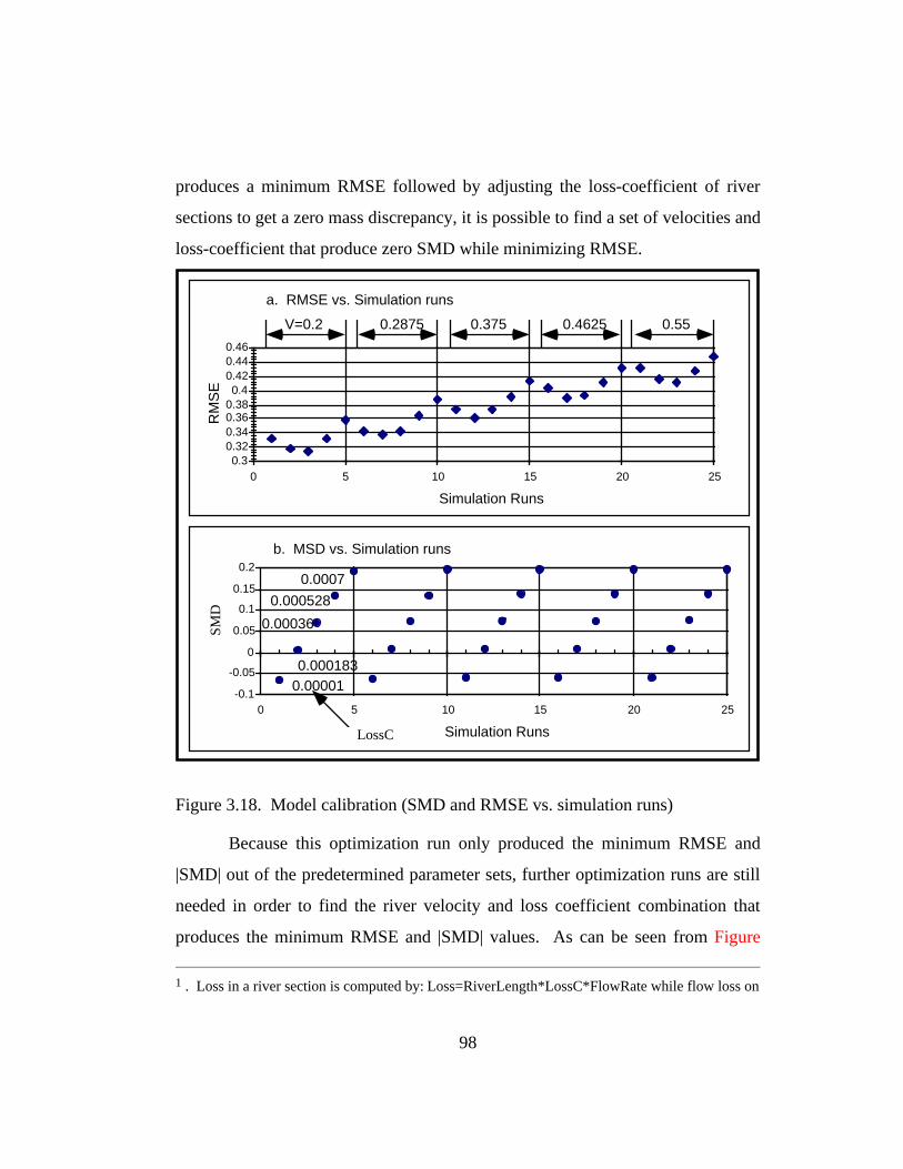
98
produces a minimum RMSE followed by adjusting the loss-coefficient of river
sections to get a zero mass discrepancy, it is possible to find a set of velocities and
loss-coefficient that produce zero SMD while minimizing RMSE.
. .
-0.1
-0.05
0
0.05
0.1
0.15
0.2
0 5 10 15 20 25
Simulation Runs
0.000010.000183
0.00036
0.000528
0.0007
b. MSD vs. Simulation runs
0.30.320.340.360.380.4
0.420.440.46
0 5 10 15 20 25
Simulation Runs
RM
SE
V=0.2 0.2875 0.375 0.4625 0.55
a. RMSE vs. Simulation runs
LossC
SMD
Figure 3.18. Model calibration (SMD and RMSE vs. simulation runs)
Because this optimization run only produced the minimum RMSE and
|SMD| out of the predetermined parameter sets, further optimization runs are still
needed in order to find the river velocity and loss coefficient combination that
produces the minimum RMSE and |SMD| values. As can be seen from Figure
1 . Loss in a river section is computed by: Loss=RiverLength*LossC*FlowRate while flow loss on

99
3.18a, the value of RMSE may still go down if river velocity is further reduced.
Because for each run, this optimization model requires a user to specify a new
range for each model calibration parameter based on the previous run, using this
interactive optimization for the simulation model calibration can be a lengthy
process.
Another problem one may face when using this interactive optimization
model is to decide the ranges of parameters for a new run after an optimization
run is done because when the number of calibration parameters is greater than
two, the plots like Figure 3.18 will not be available, and without these plots, the
patterns of RMSE and SMD variations cannot be easily detected. Because of
these problems, this interactive optimization model is never used to calibrate the
simulation model in this study. Instead, the optimization model based on a
direction set method described in the following section is responsible for all the
model parameter calibrations.
The reasons why this interactive optimization model is discussed in this
section are (1) this model provides an alternative means of simplifying model
calibration procedure when the number of parameters to be calibrated is low and
(2) this model produces charts showing the effects that each model parameter has
on the changes of RMSE and SMD (Figure 3.18) when the number of parameters
is two.
3.6.2.2. Optimization Module Based on a Direction Set Method
Using directional method, the optimization problem presented in
Equations 3.17a and 3.18a can be stated as:
a subwatershed is computed by: Loss=MeanFlowLength*LossC*PFlow

100
Given as inputs the vectors r P and
r n , and functions, RMSE(
r P ) , from
Equation 3.18a, and SMD P( )r
, from Equation 3.17a, find a scalar setλn
that minimizes RMSE(r P + λn
r n ) and satisfies SMD(
r P + λn
r n ) = 0, where
r P is a vector pointing to a point P in a N-dimensional space and
r n is the
unit vector in nth dimension of the N-dimensional space. Once the scalar
set is found, the new vector r Q =
r P + λn
r n is pointing to the point in the n-
dimensional space whose coordinates gives the optimal values of the
parameter set.
In searching for the optimal vector r Q , this optimization model uses the
bisection method (Press et al., 1992) in each dimension to perform successive line
minimization. The bisection method is used for its simplicity and reliability, i.e.
when a root is contained in a range, the root will not be lost during the iterative
root-finding procedure if bisection method is used.
Before the bisection method can be used to search for a root of a function
G(x)=0 (Figure 3.19(A)), an interval [xa,xb] containing the root needs to be
provided. For a continuous function, whether the interval contains a root can be
easily checked by testing the function values at the end points of the interval. If
the function values have different signs at the end points, then at least one root is
contained in the interval. The concept of the bisection algorithm is simple. Once
an interval containing at least one root is given, the algorithm will evaluate the
function at both endpoints and the midpoint. The endpoint giving the function
value the same sign as that of the function value at the midpoint is then replaced
by the midpoint. The procedure is repeated until the function value at the
midpoint is sufficiently close to zero. The criteria for convergence is problem

101
dependent and can usually be given by a user. For our problem of solving
equation SMD x( ) = 0 , the convergence criteria are:
SMD xmid( ) < −10 5 (3.20a)
or
( )x xk
1 2
2
+< ≈ε (3.20b)
where, x1,x2,xmid = the endpoints and midpoint of last iteration,
respectively,
ε = the convergence criterion given by a user, and
κ = a computer’s floating point precision, 10-8 for float (single precision)
and 10-15 for double precision. Similar convergence criteria is used for the
procedure that minimizes the RMSE.
Detailed discussion regarding how the convergence criteria should be set
can be found in books on numerical methods (e.g., Press et al., 1992).
Using the bisection algorithm to search for the minimum point of a
function follows a similar logic to the method used to find a function root.
Starting with a given interval [xa,xb] and xb>xa (Figure 3.19(B)), the program first
evaluates the values at the endpoints and the midpoint of the interval. If the
function value at the middle point is greater than those at the endpoints, the
program will continue on to evaluate the function points at the locations of
xa+0.25(xb-xa), xa+0.75(xb-xa), and so on, until a point whose function value is
less than at least one endpoint is found, and the point would be used as xmid. To
decide the next move, the program evaluates the function value at xtmp=xmid+dx,
where dx is a small number comparable to ε in Equation 3.20b. If F(xmid) <

102
F(xtmp), then xmid is used to replace xb to start the next iteration, otherwise, xa will
be replaced. The procedure is repeated until the function F(x) converges to its
minimum point or until the user specified maximum number of iterations is
reached.
Xa
XbXmid
xa
xmid+dx
Function F(x)
Function G(x) A
B
•
•
F(xmid+dx)
xbxmid
Figure 3.19. Using bisection method to find root and minimum points of afunction

103
3.6.3. Simulation Model Calibration
The optimization models developed in the last section are used in this
section to optimize model parameters for the purpose of simulation model
calibration.
Figure 3.20. shows the map of the Niger River Basin and the locations of
the flow-gauging stations where reasonably reliable observed monthly flow time-
series data are available for the time period between July of 1993 and December
of 1990. For model calibration purposes, five sub-models, each associated with a
flow-gauging station, are created. The optimization model based on the direction
set method is applied to each sub-model to optimize the model parameters within
its region. Based on river basin characteristic and the simulation model structure,
it was decided that six parameters affect the simulated river flow time-series.
These six parameters are listed in Table 3.3.
Table 3.5. Simulation Model Parameters To Be Calibrated
State Function (What the attribute represents)1 ToRes The fraction of a subwatershed water surplus that goes to the subsurface
reservoir2 ResK Mean residence time of water in a subsurface reservoir [T]3 VFact Overland flow velocity (m/s)4 PlossC Subwatershed loss coefficient (1/m)5 Velocity Flow velocity on a river line (m/s)6 LossC Loss coefficient related to a river line (1/m)
After applying the optimization module to the Koulikoro sub-model
(Figure 3.17) with all six parameters selected it was found that the parameters
ToRes and ResK have little impact on the simulation results, although the
combination of ToRes=0.1 and ResK=7 produces slightly better results than other
combinations of these parameters. Therefore, ToRes=0.1 and ResK=7 are used
throughout the whole model calibration process.
104
Because both river velocity and overland flow velocity (Vfact) affect flow
distributions over the time domain, only one of them is needed for the
optimization. For model calibration, the overland flow velocity (Vfact) is set to
0.013 m/s(=46.8 m/hr) while the river velocity was used in the optimization
model to minimize the RMSE.
Because overland flow occurs mostly in the form of small streams, and
because subwatershed water loss is estimated using the formula WaterLoss =
PFlow*MeanFlowLength*PLossC, which resembles the water loss formula used
in river loss estimation, it was decided that the polygon flow loss coefficient
PlossC should be set equal to the river flow loss coefficient, LossC.
After these considerations, the river water loss (LossC) and river velocity
(Velocity) are selected as the optimization parameters for the simulation model.

105
Total Drainage Area = 2.337x10⁶ km2
Delineated from 30’’ DEM (cell size=930x930 m)with threshold=10000 cells
Figure 3.20. The locations of flow-gauging stations in the Niger River Basin
Figure 3.21 shows the converging path of RMSE and SMD of the
simulated river flow time-series at Koulikoro when applying the bisection-
optimization scheme. Figures 3.22 and 3.23 show the plot of the observed vs.
simulated flow time-series when the parameter sets obtained from the
optimization model are used. From Table 3.6, it can be seen that when the river
velocity is 0.192 m/s (row 11), and Loss-Coefficient for the river and
subwatershed is 0.000985 /km, the best fit has RMSE=0.32 and SMD=0.0000116
(row 22). These two values indicate that in a 90 month period, the simulated flow
time-series produced the same amount of mass while about 16%(=32%*0.5) of

106
the mass is incorrectly placed in the time domain when compared with the
observed flow time-series.
Figure 3.22a also shows that when using the calibrated parameters, the
model underestimates both the high and low flows. The possible explanations of
the underestimation may be the following reasons:
(1) in the simulation model, the same LossC value is applied to all the
river sections and subwatersheds in the sub-model simulated area,
(2) LossC is kept constant throughout the whole simulation period,
(3) the surplus produced by the soil-water balance model may not be
adequate to generate the observed stream flow.
The underestimation caused by reasons (1) and (2) can be corrected to
some extent by assigning spatial and temporal variations to LossC but using non-
constant LossC will make the optimization model become more complicated. The
underestimation caused by reason (3) can be corrected by either using a better
soil-water balance model with improved data sets or adopting other means to
produce soil-moisture surplus (SurpF(t)) and subwatershed runoff contribution
(PFlow(t)). The estimation can probably also be improved by reducing the sizes
of subwatershed polygons and the number of subwatersheds selected for each sub-
model.

107
.
Simulation run index numberRMSE
Changing V to minimize RMSE LossC to set SMD=0
0.30.35
0.40.45
0.50.55
0.60.65
0 2 4 6 8 10 12 14 16 18
A: The converging path of RMSE
-0.1-0.05
00.05
0.10.15
0.20.25
0 2 4 6 8 10 12 14 16 18
Simulation run index numberSMD
Changing V to minimize RMSE LossC to set SMD= 0
B: The converging path of SMD
RM
SES
MD
Figure 3.21. Using bisection method to fit two simulation model parameters(LossC and Velocity)

108
Table 3.6. Optimization of River Flow Velocity and Loss Coefficient
Index RMSE SMD P-value Parameter-optimized1 1.1312006 -0.1048283 0.0500000 Ngriver.shp,Velocity,0.05,0.4,12 0.4353920 -0.1303611 0.4000000 Ngriver.shpRatio ,Velocity,0.05,0.4,13 0.3635078 -0.1295793 0.2250000 Ngriver.shp,Velocity,0.05,0.4,14 0.3637302 -0.1295891 0.2260000 Ngriver.shp,Velocity,0.05,0.4,15 0.3926416 -0.1277653 0.1375000 Ngriver.shp,Velocity,0.05,0.4,16 0.3913918 -0.1278081 0.1385000 Ngriver.shp,Velocity,0.05,0.4,17 0.3634192 -0.1289932 0.1812500 Ngriver.shp,Velocity,0.05,0.4,18 0.3631668 -0.1290096 0.1822500 Ngriver.shp,Velocity,0.05,0.4,19 0.3612605 -0.1293339 0.2031250 Ngriver.shp,Velocity,0.05,0.4,1
10 0.3612916 -0.1293474 0.2041250 Ngriver.shp,Velocity,0.05,0.4,111 0.3610867 -0.1291775 0.1921875 Ngriver.shp,Velocity,0.05,0.4,112 0.3921203 -0.2030196 0.0007000 Ngriver.shp,LossC,0.0007,0.0013,013 0.3200113 0.1924934 0.0013000 Ngriver.shp,LossC,0.0007,0.0013,014 0.3198814 0.0100611 0.0010000 Ngriver.shp,LossC,0.0007,0.0013,015 0.3484921 -0.0924330 0.0008500 Ngriver.shp,LossC,0.0007,0.0013,016 0.3314523 -0.0402009 0.0009250 Ngriver.shp,LossC,0.0007,0.0013,017 0.3251588 -0.0148247 0.0009625 Ngriver.shp,LossC,0.0007,0.0013,018 0.3224380 -0.0023209 0.0009813 Ngriver.shp,LossC,0.0007,0.0013,019 0.3211422 0.0038874 0.0009906 Ngriver.shp,LossC,0.0007,0.0013,020 0.3217759 0.0007864 0.0009859 Ngriver.shp,LossC,0.0007,0.0013,021 0.3221004 -0.0007651 0.0009836 Ngriver.shp,LossC,0.0007,0.0013,022 0.3219352 0.0000116 0.0009848 Ngriver.shp,LossC,0.0007,0.0013,0

109
10
100
1000
10000
0 20 40 60 80 100
Time (Month)
Flow
rat
e (m
3/s)
Observed Simulated
Figure 3.22a. Observed vs. simulated flow time-series at the Koulikoro flow-gauging station (flow rate on base 10 logarithm scale)
0
1000
2000
3000
4000
0 10 20 30 40 50 60 70 80 90
Time (Month)
Flo
w r
ate
(m3/
s)
Observed Simulated
Figure 3.22b. Observed vs. simulated flows at the Koulikoro flow-gaugingstation

110
0
500
1000
1500
2000
2500
3000
1 2 3 4 5 6 7 8 9 10 11 12
Time (Month)
Flow
rat
e (c
um/s
)
Observed Simulated
Figure 3.23. Observed vs. simulated mean-monthly flow at the Koulikoro flow-gauging station
Using the same procedure, sub-models were created for the regions
associated with four other flow-gauging stations. On each sub-model, the
optimization model is used to calibrate two simulation model parameters against
the long-term (1961-1990) monthly average flow and flow time-series in a seven
and a half year representative period (90 months from July, 1983, to December,
1990). The results of these calibrations are summarized in Table 3.7.
Table 3.7. Calibration Parameter Values for the Sub-Models
Station Name Time-series LossC (1/km) Velocity (m/s) RMSE SMDKoulikoro 90 months 0.00098 0.192 0.3219 0.0000116
LongTerm 0.001 0.1656 0.1429 -0.0026Douna 90 months 0.002826 0.0656 0.3736 -0.00394
LongTerm 0.000964 0.1029 0.1997 -0.0004Dire 90 months 0.000609 0.184 0.278 -0.00134
LongTerm 0.00253 0.08 0.3735 0.000167Ansongo 90 months 0.00027 0.289 0.1986 0.00095
LongTerm 0.0002935 0.2113 0.093 -0.00287Niamey 90 months 0.000433 0.4859 0.399 0.00013
LongTerm 0.00692 0.29 0.262 -0.0008

111
3.6.4. Flow Interpolation Module
This module is created to interpolate the river flow rates to a flow-check
point object. Due to its ability to dynamically segment an arc, the module is also
used in the optimization models and dam/reservoir object construction modules to
define the location of a point object.
The flow interpolation problem can be described as: given the flow rates at
From-Node (FFlow) and To-Node (TFlow) of an arc, find the flow rate at a given
point A located on the arc (Figure 3.24). The equation used for the flow rate
interpolation at point A can be written as:
IFlowA = FFlow + (TFlow − FFlow) ⋅SL
TL(3.21)
where,
IFlowA = Interpolated flow rate at point A,
SL = river distance between From-Node and point A,
TL = river distance between From-Node and To-Node, (point a and point g
in Figure 3.24).
As shown in Figure 3.24, a river line section consists of a set of straight
line segments. Before SL can be computed, it is necessary to identify which
segment contains point A. In Figure 3.24, α and β are two angles formed by the
line segment and the lines connecting point A to the end nodes of the line
segment. It follows that if the line segment contains point A, the condition
((0 o ≤ α < 90o ) and (0 o ≤ β < 90o )) holds. This condition is referred to as
“condition-A” in this section. Otherwise, one of the angles is less than 90o , while

112
the other angle will be greater than 90o . It is also true that if the angle formed by
two non-zero vectors r A and
r B is less than 90o , we have the dot product:
r A ⋅
r B = xa xb + yayb > 0 (3.22)
Because in an ARC/INFO coverage, the x,y coordinates of a point are
readily available, the dot product and the angle formed by any to vectors can be
evaluated using Equation 3.22. Therefore, to compute SL in equation 3.21, the
flow interpolation program needs first to find out which river segment contains
point A. Using the river section given in Figure 3.24 as an example, the method
for computing SL is described below.
Starting from segment ab, the program evaluates the angles ∠Aab, and
∠Aba. Since angle ∠Aba is greater than 90o , condition-A does not hold
indicating that segment ab does not contain point A. Therefore, length ab is
added to SL. Applying the same procedure to segment bc reveals that condition-
A does not hold for segment bc either so the length of segment bc is also added to
SL. On segment cd, the program finds that condition-A holds indicating that the
segment contains point A. After adding the remaining segment cs of cd to SL, the
program uses Equation 3.21 to linearly interpolate the river flow rate to point A.

113
ab c d e
fgA
FFlow
TFlow
α β
b c d
A
s• • • •
•• • • •
••
Figure 3.24. Interpolating river flow rate at a given point
The remaining segment cs can be computed using Equation 3.23 (in reference to
Figure 3.24):
cs = cA ⋅cos(α )
=(xA − xc)(xd − xc ) + (yA − yc )(yd − yc )
(xd − xc )2 + (yd − yc )
(3.23)
3.6.5. Plotting a Longitudinal Flow Profile
The map-based model allows a user to activate tasks directly from a map,
greatly simplifying some map-oriented operating procedures. In this and the next
section, two map-oriented post-processing modules are introduced to illustrate the
strength brought by the integration of programs, maps, and databases.
To perform the hydrologic analysis of a river system, it is often necessary
to plot the longitudinal flow profile on a river. If maps and databases are not
integrated, the river sections of interest first have to be selected, then the flow
data for the selected river sections have to be extracted from the database.

114
Finally, these data have to be sorted before they can be sent out to plot. The
procedures are repeated each time a different river section is picked or flow
conditions changed. In addition to the inefficiency brought by this tedious data
extraction and data processing procedure, the curve plotted is usually not shown
together with the map, which further hinders the interpretation of the plot.
In this map-based simulation model, because a program has access to both
the maps and database tables, the longitudinal profile of any selected river
sections can be plotted with a simple click on a river section. The logic of the
plotting module is described below.
When a river section is selected, its location information is passed on to
the plotting program (SFtrplt.pst). Based on the location information and river
network connectivity kept by the From-Node and To-Node of each river line, the
program traces downstream until the outlet section of the river network is reached.
As each river section is found, the flow information related to that river section is
collected from the flow table. Because the flow data is collected at the same time
river sections are traced, the collected data set is already in the correct order to
make the plotting procedure an easy next step. As the plotting program moves
from section to section downstream, the section it reaches is highlighted on the
map, so that visually, the user can be ensured that no mistake is made in the
tracing procedure. The river sections remain highlighted when their longitudinal
flow profile plot is on display which helps with profile interpretation (Figure
3.25). When plotting of another river section is desired, the user can simply mark
the new selection by clicking at the desired location and let plotting program
perform the tasks of river section tracking, data extracting, and curve plotting.

115
3.6.6. Plotting Time-Series Data at a Selected Location
This program (SFtmplt.pst) is designed to plot the temporal distribution of
a physical parameter at a given location. Like the program designed to plot the
longitudinal flow profile, this program is also activated directly by a click of
mouse on the model maps. When the location information is passed on to the
plotting program, the program uses the location information (location ID) to select
the time-series (vector) associated with the location and make a plot like that
shown in Figure 3.25. The program is designed to work with the spatially-
referenced time-series data stored in a database table with the data structure
described in Section 3.3.

116
Figure 3.25. Plotting flow distributions with the map-based surface water flowsimulation model

117
3.7. CHAPTER SUMMARY
The map-based surface water flow simulation model is constructed based
on the concepts of object-oriented programming and GIS. The model is designed
in such a way that all three components of a model, programs, maps, and
databases, are integrated.
The basic maps of the map-based model are an arc coverage containing the
river lines and a polygon coverage containing the subwatershed polygons. Both
maps can be constructed by applying a watershed delineation procedure to a
digital elevation model (DEM) of the study region. A sequence of map operations
and data structure modifications are performed on these two coverages by a set of
pre-processor programs to create river objects, subwatershed objects, and finally,
a river network. The connectivity of the river network is maintained by the From-
Node and To-Node of each river section on the network. The river sections and
subwatershed polygons have a one-to-one relationship.
To simulate river flow, the attributes FFlow and TFlow (FFlow(t) and
TFlow(t) for unsteady state) are created for each river object to hold the flow rates
at the From-Node and the To-Node of the stream line object. For each
subwatershed, PFlow (PFlow(t) for unsteady state) is created to represent the
subwatershed’s local runoff contribution. The basic relationships between these
three quantities are established based on the principle of continuity and are given
by Equations 3.1a, 3.1b and 3.2.
The sequential order by which each subwatershed in the stream network is
simulated is constructed by a stack-based stream network analysis algorithm
developed for this simulation model. The design of this stack-based stream
network analysis algorithm is based on the connectivity established by the From-

118
Node and To-Node of each arc in the network. After the sequential order is
decided, Equations 3.3 through 3.12 given in Section 3.4.2. are used to establish
the relations between PFlow(t), FFlow(t), and TFlow(t) and simulate water
movement on the river network.
Since the stack-based stream network analysis algorithm can be applied to
any stream network that fits the assumptions given at the beginning of this
chapter, it can be used to simulate other environmental processes as well. For
example, if PFlow(t) represents some pollutant sources defined on a polygon
object and the pollutant transport mechanism can be established on the rivers, the
pollutant mass loading time-series FFlow(t) and TFlow(t) associated with the
From-Node and To-Node can be simulated the same way that water flow is
simulated. In fact, the process that this model simulates may vary with the type of
model used to compute PFlow(t) on each subwatershed.
The integration of programs, maps, and databases allows easy creation of
sub-models, making it possible to divide a big study region into several sub-
regions for studies with different levels of detail.
To calibrate the simulation model, two optimization models having direct
access to the maps, databases, and simulation models are constructed. Of these
two models, the interactive optimization model can be used to calibrate no more
than 3 parameters at a time because the model needs multiple runs to complete the
calibration process, and for each new run the model requires a user who relies
largely on the two-dimension plots (Figure 3.18) to define the problem solution
space.
The optimization model based on a direction set method is used for all the
simulation calibrations in this study. The optimization program is designed in
such a way that it does not put a limit on the number of parameters that can be
calibrated at one time. But when the number of parameters to be calibrated is

119
more than four, it may take a long time to complete the optimization procedure.
The model also requires a user to provide ranges for all the calibrating parameters
at the beginning of a calibration procedure.
Although SMD and RMSE (Equations 3.17 and 3.18) are used in the
optimization model to evaluate how well the observed and simulated time-series
water, the optimization program is designed in such a way that other standards
such as lag-one correlation can be easily added.
The validation procedure of the map-based simulation model is not carried
out in this study for the following two reasons:
(1) Because the main purpose of this study is to integrate the three
components of a model, the major effort has been devoted to the
design and testing of the model programs and the communications
between the programs to ensure a smooth integration. A large amount
of work is also used to create a smooth pre-processing procedure.
(2) In the Niger River Basin area, it is difficult to find a second set of the
required data time-series, such as rainfall distribution and river runoff
observations that covers the same length of time without substantial
amount of missing records.
The main program (SFlowSim.prc) is designed in such a way that its
operation is independent of the modules used to simulate PFlow(t), FFlow(t) and
TFlow(t). The model currently provides four modules for simulating water flow
on river sections. Because all these four modules are hydrological (lumped) flow
routing algorithms, this map-based surface water flow simulation model can be
categorized as a hydrological (lumped) flow routing model, comparable to other
hydrological (lumped) flow simulation models. If hydraulic (distributed or semi-
distributed) flow routing modules such as the methods based on the differential
equations of motion and continuity in an open channel (Saint-Venant equations)

120
were used, this map-based model would become a hydraulic based (distributed)
simulation model. At one point of this study, a hydraulic routing module based
on the kinematic wave routing method was designed and tested successfully to
run with the main program. The module was later disconnected from the main
program because not enough field data were available for the Niger River Basin
area to support the hydraulic routing module.

121
Chapter Four. A Map-Based Groundwater Simulation Model
In this chapter, a map-based groundwater simulation model is constructed
to demonstrate how the concepts of object-oriented programming and geographic
information system (GIS) can be applied to simulate groundwater flow. As stated
above in Chapter One and Chapter Three, the purpose for applying the concept of
object-oriented programming and the technique of GIS is to enable the integration
of the three components (programs, data, and maps) that jointly define a
simulation model.
4.1. INTRODUCTION
A map-based groundwater simulation model has all the same benefits
brought by the integration of the three components of a simulation model as a
map-based surface water flow simulation model has. In addition, it has the
following two advantages over models constructed without GIS.
A map-based groundwater simulation model and surface water flow
simulation model can be integrated through the maps they share in
common.
Because global coordinates can easily be used as the reference system for
a GIS map, the results of a map-based groundwater simulation model can
also be presented in a global reference coordinate system, which makes it
easier for the model results to be interpreted and used than when the
groundwater model is constructed in a model coordinate system whose
exact geographic location has not been precisely defined.
As described in Chapter two, this map-based groundwater simulation
model is constructed on a polygon coverage and an arc coverage (Figure 4.1). To

122
fully utilize the data structure provided by the GIS, the continuity equation in
form of Equation 2.23 is applied to the polygon objects, while the momentum
equation in the form of Darcy’s law (Equation 2.24) is applied to the boundary
line objects. With this type of design, the groundwater simulation procedure is
greatly simplified.
Just like in map-based surface water flow simulation model, the map-
based groundwater simulation model also has three modules, pre-processor,
processor, and post-processor. The task of the pre-processor is to construct the
groundwater modeling objects from ordinary GIS maps. Using the base maps
constructed by the pre-processor, the processor simulates groundwater flow on the
line objects based on the momentum equation and computes water levels on the
polygon objects based on the continuity equation (Figure 4.1). After each
simulation, the post-processor is used to analyze and display modeling results.
The post-processor is also used for model modification and data management
purposes.
4.2. THE CONSTRUCTION OF MODEL BASE MAPS
The polygon map of a map-based simulation model originates from
ARC/INFO’s polygon coverage and the line map of the model results from
applying the BUILD line procedure to the polygon coverage.

123
•
•
•
•
•
•
•
•
••
•••
Applying the continuity equation(Equation 2.23) to the volume ofwater in each polygon
Applying the momentum equation(Darcy’s Law ) to each boundaryline of the polygons (Equation 2.24)
i j
Figure 4.1. The conceptual design of a map-based groundwater model
These two ARC/INFO coverages are then processed by three pre-
processor programs. The pre-processing procedures turn the features in the
polygon and arc coverages into the cell polygon objects and cell boundary line
objects. This map-feature to object transformation is carried out in three steps:
(1) Appending new attributes to arc and polygon map features carried out
by a table modification program [GFmdfld.pre].
(2) Filling in the newly created attributes of polygons with appropriate
values to convert them into polygon objects. These include the attributes
such as hydraulic conductivity, aquifer type (confined or phreatic), top
and bottom elevation, and storativity etc. A list of polygon attributes to
be processed is given in Table 4.1. This task can either be carried out by
a program [GFplyfld.pre], or manually.

124
(3) Filling in the newly created attributes of lines with appropriate values
to convert them into line objects. A list of the line attributes is given in
Table 4.2. This task is carried out by a spatial feature analysis program
[GFlnsfld.pre].
After the maps are processed, the cell and its boundary line objects have
the states listed in Tables 4.1 and 4.2.
Table 4.1. The Attributes of a Polygon Cell Object
State Function (What the attribute represents)1 Area Area of a polygon (m2)2 Perimeter Perimeter of a polygon (m)3 Cover_ Machine-assigned polygon ID, based on which the pointers to the time-series
tables (sprVt, rchVt, headVt, dhVt, dvolVt, etc.) are constructed.4 Cover_id User assigned ID of a polygon5 KV1000 Hydraulic conductivity (m/s)6 Head0 Initial water level in a polygon cell (m)7 Rch0 Initial recharge in a polygon cell (mm/s)8 Spr0 Initial spring flow in a polygon cell (m3/s)9 Pmp0 Initial pumpage in a polygon cell (m3/s)
10 ghb0 0 indicates the polygon is not a constant head cell, otherwise, a constant head celland the value of ghb0, is the constant water level of the cell (m)
11 evt0 Initial evaporation in a polygon cell (mm/s)12 Btm Bottom elevation of a polygon cell (m)13 Top Top elevation of a polygon cell (m)14 Cnfd 0 indicates the polygon is not confined, otherwise, the polygon is confined15 SV Storativity16 headn Water level of a polygon cell at step N, (the last simulation time step) (m)17 dvol Mass inflow to a polygon at step N (the last simulation time step) (m3/s)18 sprele Spring elevation (m)19 sprK Spring flow ~ cell water level ratio-constant (m2/s)

125
Table 4.2. The Attributes of a Boundary Line Object
State Functions & Values1 Fnode_ From-node of a line2 Tnode_ To-node of a line3 Lpoly_ Machine-assigned id of left polygon4 Rpoly_ Machine-assigned id of right polygon5 Length Length of the line (m)6 Cover_ Machine-assigned id of a line7 Cover_id User-assigned id of a line8 ldx dx of a line, dx=xn-x0. dx is the x component of a boundary-line-vector (m)9 ldy dy of a line, dy=yn-y0 dy is the y component of a boundary-line-vector (m)
10 fcosx cosine of the angle between the normal vector to the left of the line and x-axis11 fcosy cosine of the angle between the normal vector to the left of the line and y-axis12 CCX x coordinate of the center point of a line13 CCY y coordinate of the center point of a line14 Slength Distance between the center points of the two polygons sharing the line (m)15 isbnd 0 indicates the line is not an external boundary, 1=a boundary line with internal
polygon on the right, -1=a boundary line with internal polygon on the left16 bndtp 0 indicates a non-flow boundary, 1 indicates a constant head boundary17 Bhead The value of constant head level if bndtp gives a non-zero value (m)18 xflux x component of water flow rate across a line (m3/s)19 yflux y component of water flow rate across a line (m3/s)
4.3. THE SIMULATION MODEL FORMULATION
The main program of the groundwater model consists of three loops,
which are a time-loop, a polygon-loop and a line-loop. The time-loop marches
through the time dimension and simulates groundwater flow situation for each
time step. The time-loop becomes an iteration-loop under steady state. For each
time step on the time-loop, the line-loop is first carried out to compute water flow
across each line object based on the piezometric heads computed at the last time
step using the Darcy’s law. Following the line-loop, the polygon-loop is carried
out to calculate the water level changes in each cell polygon object based on the
continuity equation. The functions of these three loops and their relations to each
other are shown in a program flow-chart (Figure 4.2) and in a quasi-Avenue code
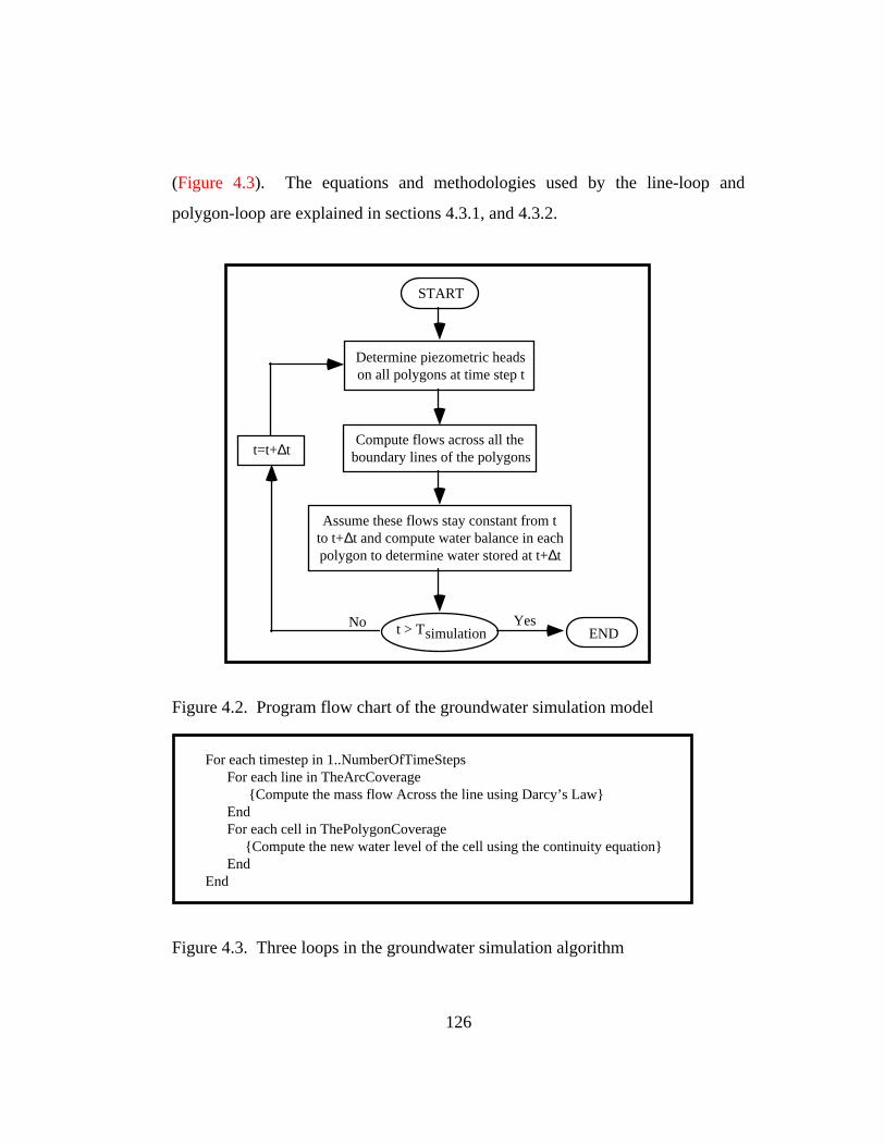
126
(Figure 4.3). The equations and methodologies used by the line-loop and
polygon-loop are explained in sections 4.3.1, and 4.3.2.
Determine piezometric headson all polygons at time step t
Compute flows across all theboundary lines of the polygons
Assume these flows stay constant from tto t+∆t and compute water balance in eachpolygon to determine water stored at t+∆t
t=t+∆t
t > Tsimulation END
START
YesNo
Figure 4.2. Program flow chart of the groundwater simulation model
For each timestep in 1..NumberOfTimeSteps For each line in TheArcCoverage {Compute the mass flow Across the line using Darcy’s Law} End For each cell in ThePolygonCoverage {Compute the new water level of the cell using the continuity equation} EndEnd
Figure 4.3. Three loops in the groundwater simulation algorithm

127
The input data sets of the model are stored either in the feature attribute
tables (FTAB) of the basic model maps or in the spatially-referenced time-series
tables associated with the basic model maps.
4.3.1. The Construction of the Line-Loop
The line-loop is constructed to simulate mass flow across each line object
to obtain the mass exchanges between two adjacent cells (Figure 4.4). For each
boundary line section, the mass flux across the boundary line from the Left-
Polygon (Lpoly) to Right-Polygon (Rpoly) is computed using the momentum
equation in the form of Darcy’s Law (Equation 4.1).
r q rl
t = −r q lr
t = −K lr ⋅dh
ds
lr
t
⋅r s lr ≈ −Klr ⋅
(hlt −1 − hr
t −1)
SLlr
⋅r s lr (4.1)
where,
r q lr
t = mass flux from Lpoly to Rpoly across the boundary line, [L/T]
r s lr = a unit direction vector pointing from Lpoly to Rpoly in parallel with
the line connecting the centers of Lpoly and Rpoly,
dh
ds
lr
t
= derivative of h in the direction of r s lr ,
K lr = hydraulic conductivity between Lploy and Rpoly in the direction of
r s lr [L/T], K
K Klr
LpolylrRpoly
lr=+
2,
Klr
Lpoly, Klr
Rpoly = hydraulic conductivities of cells Lpoly and Rpoly,
SLlr = distance between the centered points of cells Lpoly and Rpoly,
given by Slength of a line object [L],

128
hlt −1 ,h r
t −1 = water levels of cells Lpoly, and Rpoly respectively, at time step
t-1.
.
From-Node
To-Node
Right-Polygon (Rpoly)
Left-Polygon (Lpoly)
y
x
rslr
rqlr
Polygons in a polygon coveragerepresent cell objects
Arcs in an arc coveragerepresent cell boundary line objects
Internal boundary lines
exte
rnal
bou
ndar
y lin
es
Figure 4.4. The arc and polygon coverages used by the simulation model
It is assumed that the value K lr can be estimated from the hydraulic
conductivity of the cells Lpoly and Rpoly. It is also assumed that the flux lines
across a boundary line are uniformly distributed and parallel to each other. With
these assumptions, the mass flow rate across a line object can be computed by
applying the cross product to the flux vector and boundary line vector (Equation
4.2). A boundary line vector is defined as the straight line connecting the From-
Node (FNode) to the To-Node (TNode) of the line. The direction of boundary
line vector is the same as FNode to TNode direction.

129
r Q s = hs ⋅(
r q ×
r l ) = hs ⋅
r i
r j
r k
qx qy 0
lx ly 0
= hs qxly − qylx( )r k (4.2)
where, r Q s = mass flow rate across line section s [L3/T], A positive value
indicates water flow goes from Lploly to Rpoly.
r q = qx
r i + qy
r j = flux across line section s, computed using Equation 4.1
[L/T],
r l = lx
r i + ly
r j = boundary line vector of section s, [L], lx and ly are given by
ldx, and ldy attributes of a boundary line object (Table 4.1).
hs = the average depth of the aquifer at on line section s [L], Based on the
aquifer type of the adjacent cell objects, hs is computed using one
of the following equations:
(1) If both aquifers under Lpoly and Rpoly are phreatic aquifers, then
{ }h avg h b h bs l l r r= − −( ), ( ) (4.3a)
(2) If both aquifers under Lpoly and Rpoly are confined aquifers, then
hs = min (tl − bl),(t r − br ){ } (4.3b)
(3) If the aquifer under Lpoly is phreatic while the aquifer under Rpoly is
confined, then
hs = min (hl − bl ),(tr − br ){ } (4.3c)
(4) If the aquifer under Lpoly is confined while the one under Rpoly is
phreatic, then
hs = min (tl − bl),(hr − br ){ } (4.3d)
t l , t r = the top elevations of a confined aquifer under Lpoly and Rpoly,
respectively [L],

130
hl ,hr = the phreatic surface elevations of a phreatic aquifer under Lpoly
and Rpoly, respectively [L],
b l ,b r = the aquifer bottom elevations of an aquifer Lpoly and Rpoly [L].
The exchange of water volume between two polygons sharing a boundary
line section s in a given time step can be computed using:
r rV Q ts s= ⋅ ∆ (4.4)
A positive value of r
V indicates Vs is taken from Lpoly and put into
Rpoly and negative, from Rpoly to Lpoly. The volume of water exchange Vs is
used by the polygon-loop to calculate the water levels of cell objects at the end of
the current time step.
4.3.2. The Construction of the Polygon-Loop
The continuity equation used in the model to compute mass balance for a
cell object at a given time step t is given below (reproduced from Equation 2.23):
∆tt ⋅ Ai ⋅ Rit − Pi
t − Qit( )[ ]+ Vij
t
j∑ = A i ⋅Si ⋅(hi
t − hit−1 ) (4.5)
where,
∆tt = time interval at time step t,
Ai = area of cell i [L2],
Rit , Pi
t , and Qit = recharge, pumpage and discharge of the aquifer under
cell i at time step t, respectively,[L1T-1],

131
Vijt = volume of water that enters cell i through boundary j at time step t
[L3],
Si = the storativity (for a confined aquifer) or the specific storage (for a
phreatic aquifer, of cell i,
h it = water level of cell i at the end of time step t [L],
h it −1 = water level of cell i at the end of time step t-1 [L]. The water levels
of the cell objects are used by the line-loop to compute the volume of water
crossing a boundary line object for next time step.
4.3.3. Treatment of Time-Series Data Sets
The map-based groundwater simulation model uses the time-series
database tables described in Section 3.3 to store and manage all the model related
time-series data. Using this method, seven database tables are created to store the
spatially-referenced time-series data sets for the groundwater simulation model.
Table 4.3. summarizes the functions of each data table.
Table 4.3. Tables for Spatially-Referenced Time-Series Data Sets
Table Name Time Series Data [UNIT] {FieldWidth.DecimalPoints}dhtb.dbf Water level changes dh(t) of a cell object [L] {8.3}gfvtb.dbf Storage changes DV(t) of a cell object [L3/T] {14.11}headtb.dbf Water level H(t) of a cell object [L] {8.2}pmptb.dbf Pumpage P(t) applied to a cell object [L/T] {8.2}rchtb.dbf Recharge R(t) applied to a cell object [L/T] {8.2}sprtb.dbf Spring flow SPR(t) of a cell object [L/T] {8.2}xfluxtb.dbf x component of flow across a cell boundary line object [L3/T] {14.11}yfluxtb.dbf y component of flow across a cell boundary line object [L3/T] {14.11}
All the database tables listed in Table 4.3 use the same data structure in
which, the records (rows) correspond to time dimension and fields (columns)

132
correspond to the spatial features with which the time vectors are associated.
During the modeling process, the spatially-referenced time-series data are stored
and retrieved according to the time step given by the time-loop and spatial
location given by either the line-loop or polygon-loop.
4.4. TREATMENT OF MODELING CONDITIONS
As the groundwater simulation model depends heavily on the initial and
boundary conditions, this section is devoted to discuss how the initial and
boundary conditions are processed in the map-based groundwater simulation
model.
4.4.1. Treatment of Boundary and Initial Conditions
The boundary related information is stored in the Isbnd and Bndtp
attributes of a line object (Table 4.2). The Isbnd values of a line object indicate if
the line object is a external boundary line. A line object with Isbnd=0 is not an
external boundary line. A line object with its Isbnd=-1 is an external boundary
line with the exterior to its right and a line with its Isbnd=1 is an external
boundary line with the exterior to its left. Bndtp assumes a zero value for all the
internal boundary lines and no-flow external boundary lines. For constant head
boundary lines, Bndtp=1, and when Bndtp=1, the value of the Bhead attribute of
the line object gives the constant water level.
The initial conditions such as initial water level, recharge, pumpage and
spring flow, are stored with a cell polygon object. As shown in Table 4.1, initial
water level, spring flow rate, recharge rate and pumpage rate of a cell object are
stored in the attributes head0, spr0, rch0 and pmp0 of the object.

133
4.4.2. Treatment of Internal Boundary Conditions
The internal boundary conditions are used to simulate rivers and springs.
1. Treatment of Constant or Prescribed Water Level Cells
The situation of a constant or prescribed water level cell is identified by a
non-zero value of ghb0 (general head boundary) attribute associated with a cell
object. The value of ghb0 indicates the constant water level value that is
maintained through the process of simulation. Constant head cell objects can be
used to simulate rivers and springs. For a time-varying general head boundary
condition, the value of ghb0 gives the water level at the initial time step and the
time-series table (gbhtb.dbf) holds the prescribed water levels at the general head
boundary (GHB) cells for each of the following time steps.
2. Treatment of Springs
Spring flow is identified and simulated in the model by two attributes of a
cell object, SprK and SprEle. SprEle gives the elevation of the spring orifice, and
SprK gives the relation between the spring flow rate and the cell water level.
SPRK=0 indicates that no spring exist in the cell object. The spring flow can be
computed using Equation 4.6 which is formulated in a way similar to the method
used by ModFlow, (McDonald and Harbaugh, 1988).
Spr SprK (h SprEle )it
it
ii= ⋅ − (4.6)
where,
Sprit = spring flow rate on cell object i at time step t (m3/s),
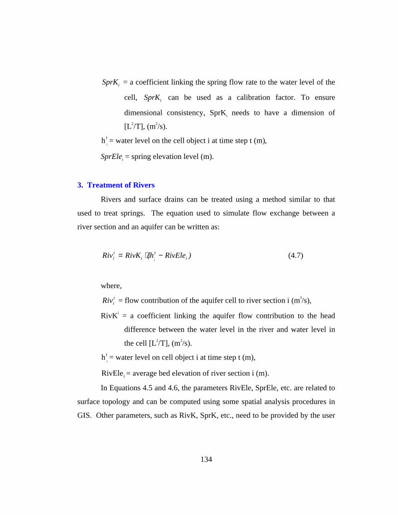
134
SprKi = a coefficient linking the spring flow rate to the water level of the
cell, SprKi can be used as a calibration factor. To ensure
dimensional consistency, SprKi needs to have a dimension of
[L2/T], (m2/s).
hi
t = water level on the cell object i at time step t (m),
SprElei = spring elevation level (m).
3. Treatment of Rivers
Rivers and surface drains can be treated using a method similar to that
used to treat springs. The equation used to simulate flow exchange between a
river section and an aquifer can be written as:
Riv RivK (h RivEle )it
it
ii= ⋅ − (4.7)
where,
Rivit = flow contribution of the aquifer cell to river section i (m3/s),
RivKi = a coefficient linking the aquifer flow contribution to the head
difference between the water level in the river and water level in
the cell [L2/T], (m2/s).
hi
t = water level on cell object i at time step t (m),
RivElei = average bed elevation of river section i (m).
In Equations 4.5 and 4.6, the parameters RivEle, SprEle, etc. are related to
surface topology and can be computed using some spatial analysis procedures in
GIS. Other parameters, such as RivK, SprK, etc., need to be provided by the user

135
or be calibrated using an optimizing procedure similar to those developed in
Section 3.6.
4.5. THE MAP-BASED POST-PROCESSORS AND UTILITIES
Using the program’s capability of having access to both model maps and
database tables, utility modules are developed so that the model related tasks such
as modifying model conditions and displaying and analyzing model results can be
performed directly from the model maps.
4.5.1. Plotting the Water Levels and Flow Distributions
This module is designed to plot water levels of groundwater cells and
water flux on the boundary lines at a user specified time step. The module is
activated by the event of either clicking on the model base map, or making the
selection from the map menu. Once activated, the module can provide
instructions to guide the user through the plotting process. Figure 4.5 shows an
example of the plotting result. In combination with the groundwater simulation
module, this water level and flow distribution plotting program is also used to plot
the water level and flow distributions for each time step on the model base maps
during the simulation process so that the model progress can be monitored on the
model base maps.
4.5.2. Plotting Time Series Data at a Specified Location
To understand the behavior of an aquifer and its simulation model, it is
sometimes necessary to plot and analyze the time-series data such as the time
variation of water level, storage, inflow and outflow at a given location. The
module of plotting spatially-referenced time-series data is designed for this
purpose. When the module is activated from the map, the location related

136
information (e.g., p(x,y)) is passed to the plotting program and based on that
information, the program first identifies the map feature that covers the user
selected point. The identification number of the selected map feature is then used
to identify the time-series vector stored in the time-series data tables. The time-
series data of a location that can be plotted for data display and analysis include:
water head level, water level changes, pumpage, recharge, and spring flows.
polygon cellsBoundary linesflux vectors
Arc coverage=> boundary lines, Polygon coverage => model cells
124.6116.184.3 84.3116.1
124.6116.184.3 84.3116.1
124.6116.184.3 84.3116.1
124.6116.184.3 84.3116.1
124.6116.184.3 84.3116.1
Figure 4.5. The water level and flow distribution plot

137
4.5.3. Modification of Model Conditions
Because the maps and databases are integrated, the model conditions of a
map-based model can be easily modified. This section describes how some of the
most commonly adjusted conditions can be changed.
1. Modification of Boundary Conditions
The boundary conditions of the model are controlled by the line object
states Isbnd, bndtp, and Bhead, where the state isbnd indicates (1) the object is not
an boundary (isbnd=0), (2) the object is a boundary line with the external region
on its left-hand-side (isbnd=1), or (3) the object is a boundary line with the
external region on its right-hand-side (isbnd=-1). When isbnd ≠ 0 , the state
bndtp is used to indicate the type of the boundary conditions, with bndtp=0
indicating a no-flow boundary condition and bndtp=1 indicating a constant head
boundary condition (flow condition). The state Bhead is used only when
isbnd ≠ 0 and bndtp=1. Under these conditions, the value of Bhead indicates the
water level at the boundary line. When simulating unsteady state groundwater
flow, the value Bhead can be allowed to vary from one time step to another with
the creation of a time-series database table. Because the model boundary
conditions are controlled by these three states of the line objects and the states of
an object can be retrieved and modified directly from a model map, the boundary
conditions can be modified directly from the model maps. The methods used to
connect the maps and the databases are logically similar to those used in the post-
processors described in Chapter Three and Sections 4.5.1 and 4.5.2 of this
chapter.
2. Modification of Pumping Situations

138
The model’s pumping condition is jointly prescribed by state pmp0 of a
polygon object and a time-series table (pmptb.dbf) associated with the polygon
objects. When modeling under steady state, the value of pmp0 indicates the
pumping rate for an object (with pmp0=0 indicating no-pumping). Under
unsteady state, the value of pmp0 gives the pumping rate at the initial stage.
Whenever pmp0 (for steady state) and pumping time-series (unsteady state)
associated with an object are changed, the model’s pumping condition is
modified. As the state and time-series table containing the pumping information
are connected to the polygon map, the method used to pass information between
maps and time-series tables described above in Section 4.5.2 is used for data
modification.
3. Modification of Recharge Conditions
The model’s recharging situation is jointly described by state rch0 of a
polygon object and a time-series table (rchtb.dbf) associated with the polygon
objects. The recharge conditions of a map-based model can be modified in the
same way the pumping conditions are modified.
4. Other Modeling Conditions
Other model conditions such as drainage and general head boundary
conditions can be treated and modified in the same way as the model’s pumping
and recharging conditions are treated.
4.6. MODEL VERIFICATION
To verify the concept and ensure the program’s correctness, the map-based
model is applied to solve the problem of groundwater flow in a phreatic aquifer

139
with accretion (dual-river-problem) (Bear, 1979) to see if model results match a
theoretical solution. The problem assumes two parallel rivers of 50 km apart and
cut into a phreatic aquifer. These two rivers can act as line sources/sinks of the
aquifer. The river levels and aquifer water level are initially at elevation of 50 m.
The aquifer has impermeable boundaries on north and south sides. An
impermeable bed is present at elevation 0 m. A uniformly distributed recharge of
1mm/day is applied on the surface. Other parameters of the example problem are
listed in Figure 4.6.
K=1m/hour
0.00 m
50.00 m
recharge N=1 mm/dayInitial aquifer water level
50000 m
RHS river providesa constant headboundary condition
50.00 m
x=0x=L
h(L)h(0)
x
Figure 4.6. A cross-section of the example problem
The continuity equation of the groundwater flow under these conditions
can be written as (Bear, 1979):
Kd
dxh
dh
dxN( ) + = 0 (4.8)
where,
K = hydraulic conductivity of the aquifer [L/T],

140
h = h(x) = water level of the aquifer at x meters from the left-hand-side
river,
N = recharge rate [LT-1].
When deriving Equation 4.8, it is assumed that (1) at the boundaries where
river intersect the aquifer (x=0 and x=L) the aquifer has vertical equipotentials
(h=h(0) and h=h(L)) and (2) every where the flow is essentially horizontal.
By integrating Equation (4.8) and considering the boundary conditions:
x=0, h h x= ( )0 and x=L, h h xl= ( ) , the shape of the water table h=h(x) can be
obtained (Equation 4.9):
( )( )
K h x h x Nx L x
Kx
Lh x h xl
[ ( )] [ ( )] ( )
[ ( )] [ ( )]
20
2
20
2 0
− − −
− − =(4.9)
where, h(x0 ) = Water level at x=0,
h xl( ) = Water level at x=L, (L=50000 meters),
N = recharge rate [L/T].
A map-based model with 5x5=25 cells is constructed to simulate the
problem (Figure 4.5) and run under the transient-state with the time-step ∆t=1day
to approach the theoretical solution asymptotically. Table 4.4 shows the water
levels produced by the map-based simulated model and theoretical solution
(Equation 4.9). The discrepancy (error% in Table 4.4) of the water levels
produced by the theoretical solution and the simulation model is measured by:

141
∆% =−dh dh
dh
t s
t
(4.10)
where,
∆% = relative error between the theoretical and simulated solutions,
dh h ht t b= − = difference between the water level at a point x and the
water level at the boundary produced by the theoretical solution,
dh h hs s b= − = difference between the water level at a point x and the
water level at the boundary produced by the simulation model.
As shown in Table 4.4 that the maximum relative error produced by the
simulation model is 3.7%. Therefore, it can be concluded that when properly
constructed, the map-based groundwater flow simulation model (GFlowSim) can
produce simulation results with reasonable accuracy (e.g., less than 5%). Figure
4.7 shows the phreatic surface profile produced by the model results and
theoretical solution. Figures 4.8 and 4.9 display the temporal variation of water
levels and net in-flow through cell boundaries. As can be seen from Figure 4.9,
when the steady state is reached, the total outflow through a cell’s boundaries at a
given time step equals the total recharges that enters the cell in the same time step.
Table 4.4. The Water Levels in the Aquifer (Simulated vs. Theoretical)
Distance Solution Simulated Solution (dh) Simulated (dh) Error%(1) (2) (3) (4)=(2)-50.00 (5)=(3)-50.00 (6)=(|(5)-(4)|/(4))*100
0 50.00 50.00 0.00 0.00 0.0005000 84.70 83.41 34.70 33.41 3.717
15000 115.90 116.50 65.90 66.50 0.91025000 124.58 124.41 74.58 74.41 0.22735000 115.90 116.50 65.90 66.50 0.91045000 84.70 83.41 34.70 33.41 3.71750000 50.00 50.00 0.00 0.00 0.000

142
.
50
83.41
116.5124.41
116.5
83.41
50
0
20
40
60
80
100
120
140
0 5000 10000 15000 20000 25000 30000 35000 40000 45000 50000
Distance (m)
Wat
er L
evel
(m
)
Theoretical solution
Model results
Figure 4.7. The phreatic surface, theoretical vs. simulated, of the dual-riverproblem
.
50
60
70
80
90
100
110
120
130
0 100 200 300 400 500
Time (days)
Wat
er le
vel
H(t) at the cell centered at x=25000 mH(t) at the cell centered at x=15000 mH(t) at the cell centered at x=5000 m
Figure 4.8. The water levels vs. time

143
-100000
-90000
-80000
-70000
-60000
-50000
-40000
-30000
-20000
-10000
0
0 50 100 150 200 250 300 350 400
Time (day)x=5000 m x=15000 m x=25000 m
Net
infl
ow th
roug
h ce
ll bo
unda
ry li
nes
(m3 )
Figure 4.9. The net in-flow through the boundaries of a cell
4.7. CHAPTER SUMMARY
The map-based groundwater simulation model is constructed using the
relations between the cells (polygons) and their boundaries (arcs) kept in
ARC/INFO polygon and arc coverages. To work within the spatial databases of
polygon and line coverages, for each time step (each iteration in case of steady
state), the model first applies the Darcy’s law to each boundary line object to
calculate the volume of water flow crossing the line. Using the volumes of the
water flow defined on the boundary line objects, together with recharge, pumping,
and spring flow time-series defined on the polygons, the continuity equation is
then applied to the polygons to calculate the water levels at the end of the time
step. The new water levels are then used to start the simulation for the next time
step. This procedure is repeated until the final time step is reached.

144
In general, the following can be said about the model:
(1) A map-based groundwater simulation model can be constructed on
any ARC/INFO polygon coverages using a set of pre-processing
programs.
(2) The modeling process can be activated and its progress monitored on
the base maps so that run time errors can be detected as they occur.
(3) Model results can be displayed on the map for interpretation.
(4) Model conditions can be modified directly from the model maps.
(5) Because in the model, the continuity equation and momentum
equations are applied separately, the model mesh can be of irregular
shape. For this reason, subwatersheds used in the surface water flow
simulation can be used by the groundwater model as its basic mesh.
(6) Because the way time-series data sets are created, the model is not
very efficient when working with a large number (about 500) of
polygons.

145
Chapter Five. Integrating Surface and Subsurface Flow Simulation
Models
5.1. INTRODUCTION
It is clear that the simulation of surface water flow of an area is not
completed until the effects of the aquifers underneath the area are taken into
consideration and the same can be said for the simulation of groundwater flow.
The interactions between surface and subsurface water flow appear in the forms of
spring flow, seepage flow, and groundwater recharge. This section describes how
these interactions can be simulated using the map-based models developed in
Chapter Three and Chapter Four.
In the map-based surface water flow simulation model, the two types of
objects used are the subwatershed object (polygon) and river object (arc). In the
groundwater flow simulation model, two basic objects are the cell object
(polygon) and the cell boundary line object (arc). Physically, the interaction
between surface water flow and subsurface water flow occurs on these line and
polygon objects. Therefore, if additional attributes (states) describing the
existence (and the types) of subsurface modeling objects can be added to the these
existing objects, the interaction between surface and subsurface water flows can
be simulated. The following section describes how the existing surface and
subsurface objects are modified so that they can be used to simulate the
interactions between surface and subsurface water flows.

146
5.2. CONSTRUCTION OF SURFACE AND SUBSURFACE SIMULATION OBJECTS
To design an integrated surface and subsurface water flow simulation
model, the spatial relationships between surface and subsurface simulation model
objects need to be defined. The relationships between surface subwatershed and
subsurface cell objects can be (1) one-to-one, (2) one-to-many, (3) many-to-one,
and (4) many-to-many. Naturally, relationships between surface and subsurface
objects tend to be one-to-many or many-to-many because surface and subsurface
objects are defined using different criteria. To simulate the interaction when
surface and subsurface objects have relations (2), (3), or (4), the simulation
program needs to add internal loops to distribute water among related objects.
To illustrate, let us assume that the integrated model is constructed with
one surface subwatershed object to many groundwater cell objects. In this case,
the spatial relationships must first be established, e.g. through the IDs of surface
and subsurface objects. After the recharge contribution of a surface subwatershed
is estimated, an internal loop is needed to distribute the recharge water to all the
groundwater cells related to the subwatershed. For the same reason, after
simulating the groundwater flow, another internal loop is again needed to
distribute aquifer discharge to their related surface objects. Although
programming techniques exist to speed up the internal loop computations, the
speed is usually accomplished at the expense of computer memory because
additional memory variables are usually needed. Therefore, an integrated model
created with surface and subsurface model having one-to-many relationships
requires either more computation time or needs more memory allocation, and
either way, the model program becomes larger and more complicated.
To avoid this complication, the integrated surface and subsurface water
flow simulation model is designed in such a way that a one-to-one relation is

147
maintained among all the simulation model objects of different classes. The task
of maintaining one-to-one relationship between the objects from different classes
is accomplished in this research by adopting the subwatershed objects used in
surface water flow simulation model as the cells for the groundwater simulation
model.
By keeping the one-to-one relationship between surface and subsurface
objects, the integrated surface and subsurface simulation model has three essential
classes of objects, which include (1) a polygon class used as both subwatershed
objects for the surface and cell objects for the subsurface water flow simulations;
(2) a river line class for surface flow simulation, and (3) a cell boundary line class
used for the subsurface water flow simulation model. The states (attributes) of
these three objects are listed in Tables 5.1, 5.2 and 5.3.
By comparing Table 5.1 with Tables 3.1 and 4.1, it can be seen that Table
5.1 is the combination of Tables 3.1 and 4.1 because in this integrated surface and
subsurface water flow simulation model, subwatershed polygons are used in both
models. Since the river line objects are not essential objects in the groundwater
simulation model, the river line objects remain unchanged. Because the cell
boundary line objects used in the subsurface water flow simulation model are not
used in the surface water flow simulation mode, they also remain unchanged.
Because the fundamental structures of the objects used in map-based
surface and subsurface water flow simulation model remain unchanged in the
integrated model, the same programs used in the surface and subsurface models
can be used in the integrated model with some small modifications. Due to this
reason, the goal of integrating the surface and subsurface flow simulation models
can be accomplished by constructing a control program that activates the map-
based surface and subsurface water simulation models constructed in Chapter
Three and Chapter Four in a proper sequence.

148
Keeping the states of essential objects unchanged simplifies the data
exchange procedure between the surface and subsurface objects. Because water
exchange between the surface and subsurface model occurs through surface
subwatershed, river line and subsurface cell objects. If these objects have one-to-
one relationship to one another, the results of one object can be directly mapped
into another, which greatly reduces the size of the model program and the model’s
computer memory requirement.
It should be understood, however, that although keeping the one-to-one
relations between the surface and subsurface objects is a way to make program
and data exchange scheme simple and efficient, it is not an essential requirement
in the design of the integrated model. The same methodology will still work
when the one-to-one relationship does not exist because program procedures can
be added to establish the spatial relationships and data exchange between the
surface and subsurface objects.
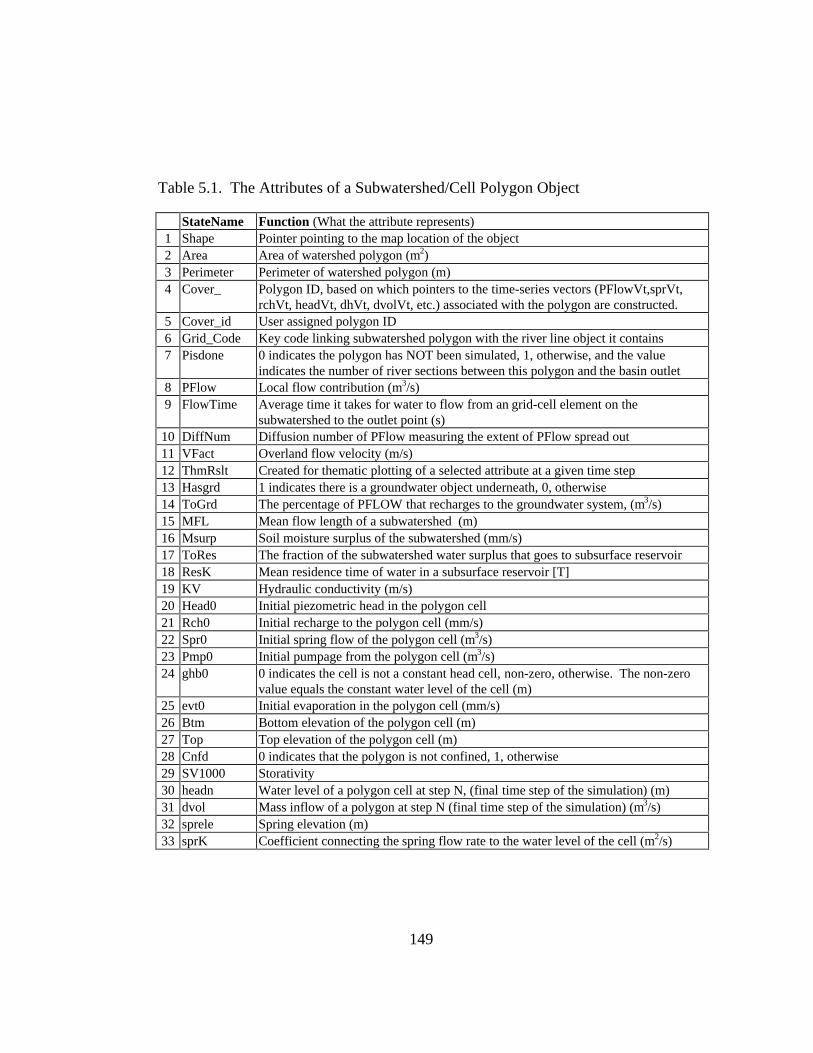
149
Table 5.1. The Attributes of a Subwatershed/Cell Polygon Object
StateName Function (What the attribute represents)1 Shape Pointer pointing to the map location of the object2 Area Area of watershed polygon (m2)3 Perimeter Perimeter of watershed polygon (m)4 Cover_ Polygon ID, based on which pointers to the time-series vectors (PFlowVt,sprVt,
rchVt, headVt, dhVt, dvolVt, etc.) associated with the polygon are constructed.5 Cover_id User assigned polygon ID6 Grid_Code Key code linking subwatershed polygon with the river line object it contains7 Pisdone 0 indicates the polygon has NOT been simulated, 1, otherwise, and the value
indicates the number of river sections between this polygon and the basin outlet8 PFlow Local flow contribution (m3/s)9 FlowTime Average time it takes for water to flow from an grid-cell element on the
subwatershed to the outlet point (s)10 DiffNum Diffusion number of PFlow measuring the extent of PFlow spread out11 VFact Overland flow velocity (m/s)12 ThmRslt Created for thematic plotting of a selected attribute at a given time step13 Hasgrd 1 indicates there is a groundwater object underneath, 0, otherwise14 ToGrd The percentage of PFLOW that recharges to the groundwater system, (m3/s)15 MFL Mean flow length of a subwatershed (m)16 Msurp Soil moisture surplus of the subwatershed (mm/s)17 ToRes The fraction of the subwatershed water surplus that goes to subsurface reservoir18 ResK Mean residence time of water in a subsurface reservoir [T]19 KV Hydraulic conductivity (m/s)20 Head0 Initial piezometric head in the polygon cell21 Rch0 Initial recharge to the polygon cell (mm/s)22 Spr0 Initial spring flow of the polygon cell (m3/s)23 Pmp0 Initial pumpage from the polygon cell (m3/s)24 ghb0 0 indicates the cell is not a constant head cell, non-zero, otherwise. The non-zero
value equals the constant water level of the cell (m)25 evt0 Initial evaporation in the polygon cell (mm/s)26 Btm Bottom elevation of the polygon cell (m)27 Top Top elevation of the polygon cell (m)28 Cnfd 0 indicates that the polygon is not confined, 1, otherwise29 SV1000 Storativity30 headn Water level of a polygon cell at step N, (final time step of the simulation) (m)31 dvol Mass inflow of a polygon at step N (final time step of the simulation) (m3/s)32 sprele Spring elevation (m)33 sprK Coefficient connecting the spring flow rate to the water level of the cell (m2/s)

150
Table 5.2. The Attributes of a River Line Object
StateName Function (What the attribute represents)1 Shape Pointer pointing to the map location of the object2 Fnode_ Node ID number of the starting point of a river line section3 Tnode_ Node ID number of the ending point of a river line section4 Lpoly_ Left polygon machine-assigned-ID (ID of the polygon to the left of the line)5 Rpoly_ Right polygon machine-assigned-ID (ID of the polygon to the right of the line)6 Length The length of the river line section (m)7 Cover_ Machine assigned river line id8 Cover_id User assigned river line id9 Grid_code Key code linking subwatershed polygon with the river line section it contains
10 LIsDone Flag 0=the river line has NOT been simulated, otherwise, simulated, and the valueindicates the number of reaches between this river line and basin outlet
11 IsHead IsHead=1, indicates a head section (the section with no upstream river lines)12 IsOutlet IsOutlet=1, indicates a outlet section (the last river line on a river network)13 FFLOW The flow rate at FNode of a river line (m3/s)14 TFLOW The flow rate at TNode of a river line (m3/s)15 Dflow The water withdrawal on the river line (diversion flow rate) (m3/s)16 Velocity Flow velocity on a river line (m/s)17 LossC Loss coefficient related to a river line (1/m)18 Timelag Flow time between the Tnode of a river line and its longest upstream flow path [T]19 MELE Mean elevation of a river line (m)20 HasDam 0 indicates no dam, non-zero indicates there is dam(s) and the non-zero value is the
dam-id of the first dam on the river line21 Hasresp 0 indicates no response function, non-zero, otherwise, and the non-zero value equals
the number of elements in the response function22 Hasgrd 0 indicates no groundwater flow model exists, 1, otherwise23 togrd The percentage of river flow that goes to groundwater recharge

151
Table 5.3. The Attributes of a Cell Boundary Line Object
StateName Functions&Values1 Fnode_ From-node of a line2 Tnode_ To-node of a line3 Lpoly_ Machine-assigned ID of the polygon to the left of the line4 Rpoly_ Machine-assigned ID of the polygon to the right of the line5 Length Length of the line6 Cover_ Machine-assigned ID of the line7 Cover_id User-assigned ID of the line8 ldx dx of a line, dx=xn-x0. dx is the x component of a boundary-line-vector9 ldy dy of a line, dy=yn-y0. dy is the y component of a boundary-line-vector
10 fcosx cosine of the angle between the normal vector to the left of the line and x-axis11 fcosy cosine of the angle between the normal vector to the left of the line and y-axis12 CCX x coordinate of the center point of the line13 CCY y coordinate of the center point of the line14 Slength Distance between the center points of the two polygons sharing the line15 isbnd 0=the line is not an external boundary, 1=a boundary line with internal polygon to
the right of the line, -1=a boundary line with internal polygon to its left16 bndtp 0 indicates a non-flow boundary and 1 indicates a constant head boundary17 Bhead The value gives the value of constant piezometric head if bndtp=118 xflux x component of water flow rate across a line (m3/s)19 yflux y component of water flow rate across a line (m3/s)
Now that the objects are constructed, the following section explains how
an integrated surface and subsurface simulation model can be constructed from
these objects under a GIS environment.
5.3. CONNECTIONS BETWEEN SURFACE AND GROUNDWATER MODELS
To integrate surface and groundwater simulation models, it is necessary
for the objects in the surface and groundwater simulation models to connect to
each other so that the outputs of one model can be used as inputs of the other. In
this simulation model, the linkage between the surface and subsurface simulation
modules is established through two state variables and a group of spatially-
referenced time-series tables. One state variable is created to store the
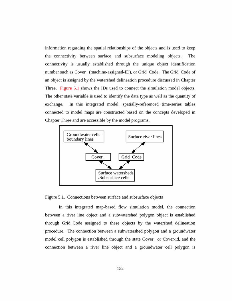
152
information regarding the spatial relationships of the objects and is used to keep
the connectivity between surface and subsurface modeling objects. The
connectivity is usually established through the unique object identification
number such as Cover_ (machine-assigned-ID), or Grid_Code. The Grid_Code of
an object is assigned by the watershed delineation procedure discussed in Chapter
Three. Figure 5.1 shows the IDs used to connect the simulation model objects.
The other state variable is used to identify the data type as well as the quantity of
exchange. In this integrated model, spatially-referenced time-series tables
connected to model maps are constructed based on the concepts developed in
Chapter Three and are accessible by the model programs.
Surface watersheds/Subsurface cells
Grid_Code
Surface river lines
Cover_
Groundwater cells’boundary lines
Figure 5.1. Connections between surface and subsurface objects
In this integrated map-based flow simulation model, the connection
between a river line object and a subwatershed polygon object is established
through Grid_Code assigned to these objects by the watershed delineation
procedure. The connection between a subwatershed polygon and a groundwater
model cell polygon is established through the state Cover_ or Cover-id, and the
connection between a river line object and a groundwater cell polygon is

153
established through Grid_Code (river) to Grid_Code (Subwatershed) to Cover_
(Groundwater Cell) (Figure 5.1).
For a river line object in the surface simulation model, two states, HasGrd
and ToGrd, and two spatially-referenced time-series tables SprVt.dbf, RchVt.dbf,
are used to store the volumes of water exchange between the objects in surface
and groundwater models for each simulation time step. The values of HasGrd and
ToGrd indicate if a groundwater unit exists underneath and if so, the recharge rate.
SprVt.dbf and RchVt.dbf are accessible by both groundwater and surface water
flow simulation models. The table, SprVt.dbf is used to store the spring flow
time-series and RchVt.dbf is used to hold the recharge time-series. In general, the
spring flow outputs of the groundwater simulation model are held in SprVt.dbf to
be used as inputs to the surface water flow model. The recharge outputs of the
surface water flow simulation model are held in RchVt.dbf to be used as inputs to
the groundwater model.
Because in the integrated surface and groundwater model, subwatersheds
used in surface water flow simulation and cells used in the groundwater model are
merged, the information can be exchanged directly through the record number of
the feature attribute table (FTAB). The states, HasGrd and ToGrd, and three
spatially-referenced time-series tables, SprVt.dbf, RchVt.dbf and PmpVt.dbf are
used to control the water exchange between the objects in surface and subsurface
water flows.
5.4. SIMULATING THROUGH THE SPACE AND TIME
Before a simulation model for a hydrologic process that occurs in the
domains of both space and time can be constructed, one has to decide the
simulation sequence over space and time (Figure 5.1). To complete the

154
simulation process, the model needs to loop through each spatial feature at each
time step. Depending on the nature of the process, a program can be designed in
such a way that the simulation model visits all spatial feature objects for a given
time step before it moves on to next time step (TIME-FIRST-THEN-SPACE), or
once the simulation model has visited one spatial feature, it simulates the process
on that feature for all the time steps before it moves on to next feature object on
the spatial domain (SPACE-FIRST-THEN-TIME).
For the map-based surface water flow simulation model, SPACE-FIRST-
THEN-TIME simulating sequence is used because (1) the flow process through
all steps in an object can be simulated using the information associated with that
object alone, and (2) the effects of an object on the river network can be replaced
by a set of flow time-series data. For the subsurface water flow simulation model,
however, TIME-FIRST-THEN-SPACE scheme is used because, a simulated
variable, e.g. water level, of all spatial feature objects at a given time step must be
calculated simultaneously before the simulation model can move on to the next
time step.
Because the surface and subsurface models designed in this study use
different simulation sequences over the space features and over time domain, the
integration of surface model and subsurface model is achieved via the data
exchanges through the time-series tables. The scheme proposed to integrate
surface and subsurface simulation models is discussed in Section 5.5.

155
Time
0
1
2
3
4
5
Spatial Features
Figure 5.2. The spatial and time domains of a simulation model
5.5. INTEGRATION OF SURFACE & SUBSURFACE WATER FLOW SIMULATION
MODELS
As discussed in Section 5.4, the integration of the surface and groundwater
simulation model is to be accomplished through the spring flow and recharge
time-series tables created to hold the volumes of water exchanges between these
two models. During a simulation, the spring flow time-series produced by the
groundwater model is used as input by the surface flow simulation model and the

156
recharge time-series produced by the surface flow simulation model is used as
input by the groundwater simulation model. Because the same simulation
sequences used in map-based surface water flow simulation model and subsurface
water flow simulation are used in the integrated model, the integration scheme
proposed above can be accomplished by using a short main program to call
alternately the map-based surface and subsurface simulation models.
To illustrate the general simulating procedure for an integrated model, let
us assume that the model starts with surface water flow module. It is clear that
spring flow time-series is needed to simulate the surface water flow. Because
spring flow comes from the groundwater simulation model that has not yet run, an
initial estimates of spring flow are needed. Once the spring flow time-series are
estimated, the surface water flow simulation can proceed. As a result of surface
water flow simulation, recharge flow time-series are produced. The recharge flow
time-series are then used as inputs by the groundwater flow simulation model to
complete the groundwater simulation. As a result of this groundwater simulation,
a set of spring flow time-series are produced. The spring flow time-series are
compared with the estimated spring flow time-series to check for discrepancies.
If the discrepancies are small, the simulation results will be deemed as converged
and the simulation procedure will be stopped. Otherwise, the newly simulated
spring flow time-series will be used for the surface water flow simulation model
for the next iteration. The procedure is repeated until the spring flow time-series
converges or the maximum number of iterations specified by a user is reached.
The procedure described above is illustrated in Figure 5.3.

157
Initial conditions for surfaceand goundwater simulationmodel + initial estimates ofspring flow time-series(value(0))
Run the surface model to obtainsubwatershed local runoff andflow time-series at Fnode andTnode of a river section
If(Value(o)-Value(n)) < e
Yes
Simulation completeStop and Exit
No
If(n >Nmax)
Doesn’t convergeExit (write results)
Yes
No
Value(o)=Value(n)(discharge(o)=dischage(n))
Run groundwater model toobtain groundwater levelsand spring flows (value(n))
value(0)=initial estimatesvalue(n)=produced by the simulation model after n iterations
Figure 5.3. Simulating procedure of an integrated model
5.6. AN APPLICATION EXAMPLE OF THE INTEGRATED MODEL
Using the procedure described above, the integrated model is applied to
the Iullemeden region of the Niger River Basin to simulate the surface and
subsurface water flow interaction. The groundwater simulation module of the
integrated model is constructed from the map-based surface simulation model
using the subwatershed polygons of the surface water flow model as its model

158
cells. The study region and the physical parameters of the map-based Iullemeden
model (Map-Based model) are extracted from a Modflow groundwater model
(Modflow model) constructed for the same region by the Food and Agriculture
Organization (FAO), (Guerre, 1995). The study region of the Modflow model is
discretized into a 60r x 42c cells with the origin at the upper-left corner of the
region. The sizes of the cells from row 1 to 35 are dx*dy=20*20 (km) and those
of the cells from row 36 to 60 are: dx*dy=20*10 (km). Based on the Modflow
model conditions, a map-based Iullemeden groundwater model of 60 polygons is
constructed. The procedure used to construct the map-based Iullemeden model is
given below:
(1) Using the INTERSECT function of ARC/INFO, the polygon maps
(NGBASIN) used in the surface water flow simulation model is
intersected with the groundwater model mesh (IUPOLYPJ) to create
intersected converge INTIUPLY. The purpose of this map operation
is to create spatial relationships between the subwatershed polygons
and Modflow model mesh (Figure 5.4).
(2) Selecting all the subwatersheds that intersect with the mesh of
Modflow model and assigning their HASGRD state value to one
(HASGRD=1) indicating that there is a groundwater aquifer below.
With HASGRD=1, when the surface water flow simulation model
runs through these polygons, recharges will be evaluated (Figures 5.4
and 5.5).
(3) Running the program (GFlnsfld.pre) to select all boundary lines of the
subwatersheds that will be used as groundwater cells, setting
HASGRD state of these boundary lines to one (HASGRD=1), and
defining the external boundary line of the groundwater model
(Figures 5.4 and 5.5).

159
(4) Using the intersect coverage, the converting program
(CONVERT.UTL) is applied to extract model parameters, initial and
boundary conditions from the Modflow model and put into the Map
based model. These parameters include: hydraulic conductivity, the
aquifer’s bottom and top elevations, initial water level, pumpage,
evaporation, and a recharge time-series.
The Modflow model also produced a spring flow time-series at cell
(48r,13c) (Figure 5.7). Cell (48r,13c) is contained in subwatershed GC116 in the
map based model. The purpose of applying the Map based model is to see if the
map-based model can reproduce the spring flow time-series at the designated
location under a similar modeling conditions as those used by the Modflow
model. The Modflow groundwater simulation model is used to evaluate the
model result of this map-based flow simulation model because the Modflow
model is most widely used and tested among all groundwater simulation models
(Anderson and Woessner, 1992).

160
Figure 5.4. The study area of the map-based and Modflow Iullemedengroundwater models

161
Figure 5.5. The polygons of the map-based groundwater simulation model
As discussed above in Table 5.1, the parameters that control the spring
flow time-series of the map based model are SPRELE and SPRK. The parameter,
SPRELE gives the elevation of a spring orifice and SPRK is a coefficient that
relates the head difference between the aquifer water level and the elevation of the
spring orifice to the spring flow rate. In the map based model, SPRK is also used

162
as an logical variable to indicates if a subwatershed polygon has a spring
(SPRK≠0) or not (SPRK=0).
Using the data sets extracted from the Modflow model and under the
surface water flow simulating conditions (Chapter Three) for the 90 month period
between July, 1983 and Dec, 1990, the map-based model are tested with different
sets of SPRK. The spring flow time-series produced by (SPRK=7.46 m2/s) is
given in Figure 5.6. The monthly average spring flows produced by the map
based model over the seven and half year period are listed in Table 5.4 and
compared with those produced by the Modflow model. The last column in Table
5.4 is computed using a formula similar to Equation 4.10 to show the relative
difference between the spring flow rate produced by the map based model and
those produced by the Modflow model.
Table 5.4. The Monthly-Average Spring Flows at GC116 Produced by the MapBased Model and at Cell (48,13) by the Modflow Model
Month Modflow (m3/s) Map-Based (m3/s) error%
(1) (2) (3) |(2)-(3)|/(3)
January 1.000 0.971 2.900
February 2.200 2.158 1.909
March 6.100 6.025 1.230
April 8.600 8.507 1.081
May 9.700 9.604 0.990
June 10.800 10.701 0.917
July 9.500 9.414 0.905
August 3.100 3.047 1.710
September 1.900 1.851 2.579
October 1.300 1.252 3.692
November 2.600 2.547 2.038
December 1.400 1.348 3.714

163
The results listed in Table 5.4 show that the differences between the
monthly average spring flows produced by the Map based model and those
produced by the Modflow model are within 4%. The spring flows produced by
the Map based model and Modflow model are plotted in Figure 5.7.
Although in running the map-based integrated model, the recharge data
extracted from the Modflow model are used directly and not produced by the
map-based surface water flow simulation model, the surface water flow
simulation model has the ability to reproduce the same set of recharge data by
adjusting the TOGRD attribute of each subwatershed polygon and river line
object.
0
2
4
6
8
10
12
0 10 20 30 40 50 60 70 80 90
Time : July, 83 - Dec., 1990 (month)
Figure 5.6. The spring flow time-series at GC116 produced by the Map basedmodel

164
0
2
4
6
8
10
12
1 2 3 4 5 6 7 8 9 10 11 12
MonthModflow Map-Based
Figure 5.7. The monthly-average spring flows at GC116 produced by the Mapbased model and at cell (48,13) by the Modflow model
5.7. MODEL INTEGRATION - CONFINED VS. PHREATIC AQUIFERS
In general, a phreatic aquifer close to the surface will work interactively
with surface water. Therefore, in simulating the interaction between the surface
water and a phreatic aquifer, the subwatersheds used as model units for surface
water flow simulation should also be used as groundwater simulation units to
simplify the water exchange procedure. On a phreatic aquifer, the locations and
discharge rates of groundwater contribution to surface water flow can usually be
jointly determined by the aquifer water levels and surface water levels. Because
these values are simulation model results, they are unknown until the simulation
model is run. In other words, the recharge/discharge locations and quantities are
“computed” by the simulation.
For a deep aquifers, however, the surface and groundwater water exchange
is usually determined by both geological formations and piezometric heads in the

165
aquifer. Because the geological formation has to be given, the possible locations
of recharge and discharge (spring flow) need to be given prior to the simulation.
The simulation model is then used only to determine the quantities of the water
exchange. Therefore, for a deep aquifer, it may not be appropriate to use
subwatershed polygons as the groundwater model cells. Because surface water
flow in most cases is of single direction, recharge to the groundwater can be
determined by the surface water flow simulation, which makes it possible to run
the groundwater model separately from the surface model and using the time-
series data tables (SprVt.dbf and RchVt.dbf) pass the water exchange after each
run. In this way, the surface and groundwater water models are coupled only
through the data exchange and in most cases.
The program section that simulates the water exchanges between surface
and subsurface water would remain largely unchanged for both phreatic aquifer
and confined aquifers. The differences in simulating water exchanges lies mainly
in data preparation. To simulate water exchange between a phreatic aquifer and
surface water flow, one can simply provide the initial water levels of aquifer and
let the simulation model determine the location and quantities of water exchange.
To simulate water exchange with a confined aquifer, one needs to provide
additional information regarding the locations and characteristics of the springs
and recharge points before the simulation model can be constructed.
5.8. CHAPTER SUMMARY
This chapter explores the possibilities of integrating the surface and
subsurface water flow simulation models using the concept of object-oriented
programming and GIS techniques. The results of this research can be
summarized below:

166
1. In constructing the map-based flow simulation models in this research,
the surface water flow is described by a river network analysis
algorithm while the groundwater flow is described by a two
dimensional potential flow equation. Because of this difference, the
simulation programs for these two problems are self-contained and use
different simulation procedures through space and time. Therefore, it is
difficult and inefficient to integrate the two simulation models into a
single program entity.
2. Because of these differences in surface and subsurface water flow
simulation models, the integration of these two models needs to be
accomplished through the modeling data sets. Two databases, recharge
and spring flow time-series tables, that these two simulation models
both share, can be used for data exchange purposes.
3. The connectivity of the surface and subsurface modeling objects can be
established through some properly constructed states of these objects
(Tables 5.2 and 5.3).
4. When the subwatersheds of surface water flow simulation model and
cells of subsurface water flow simulation model do not have the same
shapes and sizes, the spatial relationships between surface and
subsurface modeling entities may be established through some GIS map
operating procedures such as INTERSECT and UNION. Using these
relationships, the results of one model can be converted and used as the
inputs for another model..
5. When using the proposed method (i.e. model integration through data
exchange) to integrate surface and subsurface simulation models,
because surface water flow simulation needs aquifer discharge as its
input and groundwater flow simulation requires recharge as its input,

167
one of these time-series needs to be estimated or known to start the
simulation. If estimated values are used, the simulation procedure
needs to be iterated until the modeled time-series converged.
6. Although by adjusting the values of SPRK, the map-based ground-
water model can generate correct spring flow time-series for the map-
based surface water model, the water levels produced by the map-
based groundwater model are not as accurate when compared to those
calculated by a Modflow model, because in an integrated model, the
areas of the groundwater computation units (polygon cells) are too
large.

168
Chapter Six. Summary and Conclusions
As stated in Chapter One, the principal purpose of this research is to
design map-based surface and subsurface simulation models that have all three
model components - programs, maps and databases - integrated. As a result of
this research, a map-based surface water flow simulation model and a map-based
groundwater flow simulation model are constructed. Both models are based on
the concepts of object-oriented programming (OOP) and geographic information
systems (GIS). Listed below are conclusions that can be drawn from this
research:
1. Using the concepts of object-oriented programming and relational
databases, it is possible to design an efficient map-based simulation
model for surface and subsurface water flows under the environment
of a geographic information system (GIS).
2. In order to design a map-based flow simulation model under GIS
environment, it is necessary to design an efficient data structure to
manage the spatially-referenced time-series data. A data structure has
been designed and used successfully to manage all the spatially-
referenced time-series data sets for the simulation models. The data
structure has the following features (Chapter Three):
(a) One data table is created for each data item with the table name
reflecting the item name.
(b) The fields (columns) are related to the spatial features on the map
with the field names constructed from the feature identifications.
The number of fields equals the number of features on the map that
have time-series data defined on them.

169
(c) The records (row) of the table store the time steps of the spatially-
referenced time-series data.
3. Due to the integration of its three model components, the map-based
surface water flow simulation model has the following capabilities:
(a) The base maps of the model and the simulation model itself can be
constructed using an interactive and menu-driven user interface.
Thanks to the programs developed for the base map and simulation
model construction, this map-based water flow simulation model
can be recursively applied to different regions with very little
model modification.
(b) Once the base maps and the simulation model are constructed, the
modeling procedure can be activated from the maps with its
progress being monitored on the maps.
(c) The model results can be displayed, retrieved, and analyzed on the
maps. Displaying and analyzing the model results on the model
maps make it easier for a model user to understand and interpret
the model results.
(d) Model conditions can be modified directly from the maps, i.e.
when a map is altered, its associated data tables and programs will
also be modified accordingly to reflect the change. Due to this
type of model design, a portion of study region (subregion) can be
isolated and cut to create a “sub-model” for more detailed analysis.
4. The experience of constructing these map-based models shows that the
“one-to-one” condition imposed on the relationship between objects
among different classes can greatly improve the efficiency and
portability of the model programs. In fact, it is generally true that
when applying the concept of object-oriented programming to

170
construct a model, it is more efficient to use combinations of many
simple objects rather than to use a single complex object to simulate
complex situations. If the simple-single object method is used, a new
complex situation can usually be simulated with the combinations of
these simple-single objects or with the creation of new simple-single
objects, while if a complex single object is used then it may not be
reusable for another new situation because it is inefficient, if not
impossible for an already complex object to be modified to fit a new
situation.
5. The map-based groundwater simulation model is constructed by
applying the continuity equation (Equation 2.23) to the polygons and
the momentum equation (Darcy’s Law) to the boundary lines of these
polygons. Because such a design is consistent with the data structures
of the polygon and line attribute tables in ARC/INFO GIS, the model
and its data sets are fully integrated with the basic maps. In addition to
the features listed above for the map-based surface water flow
simulation model, the following features are specific to the
groundwater simulation model:
(a) The base maps and model can be constructed from a given polygon
coverage.
(b) The meshes (polygons) used for the simulation model can be of
any shape, which makes it possible for groundwater model meshes
to take the shapes of subwatershed polygons of the surface water
flow simulation model.
(c) Under this design, the continuity and momentum equations are
defined separately on the polygon and polygon boundary line

171
objects and the problems of assembling and solving large set of
linear equations are avoided.
6. The application of the concepts of object-oriented programming and
GIS approach makes it possible to construct a model not in terms of
state variables but in terms of problems and problem objects.
7. The one-to-one relationship between the surface and subsurface objects
are emphasized in designing the integrated surface and subsurface
water flow simulation model. A simulation model procedure that
keeps the one-to-one relationship between the modeling objects can
greatly simplify the data exchange procedure and make the simulation
program efficient. Technique exist, however, to design an integrated
model with one-to-many type spatial relationships. For example, if it
is desired to have a model with one surface object to many
groundwater objects, the model can be designed as described below.
Two pointer states can be created for each of the subsurface objects
and one for each of the surface objects. The first pointer of a
subsurface object is used to point to next subsurface object that is
spatially connected to the same surface object. A zero value of the
first point indicates that the object is the last of the subsurface objects
connected to the same surface object. The second pointer of a
subsurface object is used to point to its connected surface object. The
pointer of a surface object is used to point to the first of the subsurface
objects connected to it. This way, a surface object only needs to know
the first in the list of subsurface objects that are related to it, which
converts the original one-to-many relation into a one-to-one relation.
8. Because the map-based surface and subsurface models are constructed
based on the map topology of ARC/INFO, the model programs must

172
be designed internally within the ArcView environment. Although
using the programs internal to ArcView greatly enhances the models
graphical presentation, e.g. allowing the simulation results to be
monitored and displayed on the base map while the simulation is in
progress, the model runs slowly when compared to models written
with external programming languages, such as FORTRAN and C++.
Possible solutions to the problem of model speed could be found by
either exporting the ARC/INFO map-topology for use by external
programs or creating other ways to connect the model objects for use
in external programs.
With the successful design and construction of these map-based simulation
models, this research has shown that using the techniques of object-oriented
programming, relational databases management, and GIS, it is feasible to
construct a model with all three of its components integrated. By applying the
model to the Niger River Basin, this research has also demonstrated the
effectiveness of the map-based model in surface water flow simulation.

173
Appendix I. The Map-Based Surface Water and Subsurface Water
Flow Simulation Models
User’s Manual
1. MODEL INSTALLATION .............................................................................. 173
2. MODEL DESCRIPTION................................................................................. 173
2.1. General description .......................................................................................................173
2.2. The construction of base-maps and spatially referenced time-series data sets ..............175
2.2.1. Construction of model base-maps ..........................................................................175
2.2 The maps of the simulation model .................................................................................184
2.3. The Model’s Graphical User Interface ..........................................................................186
2.3.1. View Menu.............................................................................................................186
2.3.2. View Button Bar ....................................................................................................189
2.3.3. View Tool Bar........................................................................................................190
2.4. Model programs ............................................................................................................192
3. PERFORMING TASKS UNDER SFLOWSIM/GFLOWSIM .............................. 197
3.1. Surface Water Flow Simulation ....................................................................................197
3.2. Creating Dam/Flowchk/Diversion objects ....................................................................198
3.3. Interpolating the Flow Rates to Flowchk Points............................................................199
3.4. Plotting Surface Water Flow Profiles............................................................................199
3.5. Plotting Groundwater Flow Related Items ....................................................................199
3.6. Creating a Sub-Model ...................................................................................................199
3.7. Model Parameter Optimization (Model calibration) .....................................................200
3.8. Map-Based Groundwater Model ...................................................................................201
3.9. Writing Scripts Contained in the Project to Disk ..........................................................202
3.10. Creating Time Series Database Template ...................................................................202
3.11. Setting up Model’s Control List ..................................................................................202
3.12. Running the Groundwater Simulation Model..............................................................203
3.13. Other Programs ...........................................................................................................203

174
1. Model Installation
All model programs are contained in the project file HYDRO.APR. To test the model,
two coverages in ARC/INFO export format are provided. These two files are NGBASIN.e00 and
NGRIVER.e00. NGBASIN.e00 contains subwatershed polygon and polygon boundary line
coverages of the Niger river basin in the west Africa and NGRIVER.e00 contains the river line
coverage of the Niger river basin. These coverages are created by applying a delineation
procedure to the 5 minute DEM of the region. The delineation procedure are given in Figure 2.
To install the coverages on a UNIX workstation, from under the ARC/INFO’s ARC
prompt, type in:
IMPORT COVER NGBASIN NGBASIN and
IMPORT COVER NGRIVER NGRIVER
To install the coverages on a PC with ArcView version 2.1 or later, from DOS prompt,
type in:
IMPORT C:\WIN32APP\ArcView\BIN\IMPORT.EXE C:\NGFLOW\NGBASIN.E00
C:\NGFLOW\NGBASIN and
IMPORT C:\WIN32APP\ArcView\BIN\IMPORT.EXE C:\NGFLOW\NGRIVER.E00
C:\NGFLOW\NGRIVER
assuming your ArcView is installed under C:\WIN32APP, your *.E00 files are in
C:\NGFLOW and your coverages are to be stored under C:\NGFLOW.
After restoring these coverages, following the procedure described on next section to construct and
run the map-based surface water and groundwater flow simulation model.
2. Model Description
2.1. GENERAL DESCRIPTION
The integrated map-based surface and subsurface water flow simulation model is
contained in the HYDRO.APR project. To construct a map-based surface and subsurface water
flow simulation model for a region (using the Niger River Basin as an example), three coverages
are required, a polygon coverage (NGBASIN), a line coverage constructed using the ARC
command: build NGBASIN line, from the NGBASIN polygon coverage, and NGRIVER line

175
coverage. All these three coverages are created by applying the watershed delineation procedure to
the DEM’s in the Niger river basin area. Figure 1. shows the components of a map-based surface
water flow simulation model.
Regional DEM lattices(Raster based GIS)
Watershed delineationprocedure
River line and watershedpolygon coverages(Vector based GIS)
Map-operating procedures * create river line object * create watershed object * construct stream network * establish one-to-one link between river lines and watershed polygons
Suitable for spatial analysis
Suitable for network analysis
Map-Based Surface Flow Simulation Model Processor
Pre-processor
Flow distribution display
Constructor of the riverflow diversion objects
Constructor of the dam/reservoir objectsFlow-check point constructor
Baby-model constructorOptimization program formodel parameter-fitting
Utility programsPost-processor
Avenue programsSpatially-referencedtime series data sets
Base Maps
Figure 1. The components of a map-based surface water flow simulation model

176
As shown in Figure 1, a map-based surface water flow simulation model is supported by
both spatial-data sets (maps) and spatially-referenced time-series data sets. Section 2.2 describes
both the model base-map construction procedure and the time-series data preparation procedure.
2.2. THE CONSTRUCTION OF BASE-MAPS AND SPATIALLY REFERENCED TIME-SERIES DATA SETS
2.2.1. Construction of model base-maps
Step 1. Applying watershed delineation procedure to the DEM of the study region.
The base-maps are acquired by applying a watershed delineation procedure to the digital-
elevation model (DEM) of the region. Figure 2 gives a sample river basin delineation procedure.
‘***********************************‘A sample delineation procedure - deline.aml‘***********************************demprj = project ( demorg, project. prj, #, 100)fill demprj demprjdemfdr = flowdirection ( demfil )demfac = flowaccumulation ( demfdr )&sv thres =10000demstr = con(demfac > %thres%, 1)demlnk = streamlink ( demstr, demfdr)NGRIVER = streamline ( demlnk, demfdr, grid-code, #)demacc = zonalmax ( demlnk, demfac)demout = con (demacc == demfac, demlnk)demshd = watershed ( demfdr, demout)NGBASIN = gridpoly ( demshd )quit
Figure 2. A sample delineation procedure
As a result of applying the delineation procedure, two coverages are generated,
NGBASIN representing the subwatershed polygons and NGRIVER representing the river lines.
Since the GRIDPOLY function produced only the polygon coverage, the following ARC command
needs to be applied to build the accompany line coverage:
BUILD NGBASIN LINE

177
Step 2. Dissolving the single-cell-polygons
To dissolve the single-cell-polygon, using the ARC command:
DISSOLVE incov outcov GRID-CODE poly
This command dissolves all the single-cell polygons into its adjacent polygons with the same grid-
code that share at least one common boundary line. Because some single-cell polygons share no
common boundary with their adjacent polygons, they will not be dissolved by the ARC’s
dissolving procedure. In this case, NGBASIN.ply, NGBASIN.lin and NGRIVER need to be added
to the HYDRO.apr so that the SFdslv.pre (avenue program designed to modify the GRID-CODE
assignment) can be applied to the NGBASIN.ply. To add the themes to an active view, use the
button from the View button bar. Once all three coverages are added, using the button
to setup the control data sets (associated with the project-level ObjectTag). Once this is done, click
the tool from the View tool bar followed by click on the cursor-sensitive area of the view
that contains NGBASIN.ply, NGBASIN.lin, and NGRIVER themes. When prompted with the list
of the programs that are available from the tool, select the program SFdslv.pre, which will
reassign the appropriate grid-code values to all the single-cell polygons so that they will share a
common boundary line with their adjacent polygons.
After running SFdslv.pre, exit ArcView and from ARC, apply the DISSOLVE procedure
again, which should dissolve all the unwanted single-cell-polygons.
Step 3. Modifying the feature attribute tables (FTABs) of the subwatershed polygon and
river line coverages (SFmdflds.pre)
The purpose of adding additional fields to the FTABs is to create river line and
subwatershed polygon objects for the map-based surface water flow simulation model. The
procedure starts with using the button from the View button bar to add NGBASIN.ply,
NGBASIN.lin, NGRIVER to an active-view, then from View menu bar, click SFwModel, and
select MdfyFtabs(pre-1). The program will prompt the user to select from a list of the themes the
names of river line coverage (NGRIVER), subwatershed polygon coverage (NGBASIN.ply) and
subwatershed boundary line coverage (NGBASIN.lin) and proceed to add the necessary attributes

178
to these three coverages. The program SFmdflds.pre also sets up the control-list and attaches the
list to the project-level OBJECT-TAG. The control-list is shown below in Figure 3. Items are
delimited by “=”.
NGBASIN.ply=NGBASIN_=Grid_Code
NGRIVER.shp=NGRIVER_=Grid_Code
NGBASIN.lin=NGBASIN_
Figure 3. Control-list set to the object-tag at the project level (3 parameters)
Step 4. Sorting nodes and vertices of river lines [SFsortr.pre].
This procedure sorts the nodes of the river lines so that the direction of From-Node
(FNode) to To-Node (TNode) (Figure 4) of a river line section is always pointing in the
downstream direction. The program also sorts the vertices of a river line so that the vertex with
zero-index is located at the FNode of the line. Before the sorting program could be run, you need
to identify the outlet river section by setting the attribute ISOUTLET of the outlet section to 1
(one). To do this, make sure the river theme (NGRIVER) is active and visible. Then from View
button bar, click the button to get the FTAB associated with the river theme and while the
F-Table is active, click the button to promote all the selected records to the top and change
the ISOUTLET attribute to 1 (one). Once this is done, the sorting procedure can start. To perform
the task of sorting, click SFwModel followed by selecting menu item LineSortR(pre-2).
When running SFsortr.pre, an error message (something like ERROR ON EXECUTING
LINE X ON PROGRAM XXXX.c) may appear, which may be caused by the protection of
NGRIVER coverage. When this happens, we need to used the CONVERTTOSHAPEFILE option
from THEME menu from the View menu bar to covert NGRIVER coverage to a shape file with
the same name. Then add the NGRIVER.shp file to the view as a new theme, reset the control-list
by clicking at and select NGRIVER.SHP and the river theme. Then rerun the program
SFSortR.

179
5
6 7
8 9
10
(a) Line presentation of a riversection created by delineation
5
10
5
6 7
8 9
10
(b) After correcting node ordering
(c) After merging the segments
Figure 4. Sorting and merging multiple river segments into one river section
Step 5. Cleaning the river line splits (SFsplit.pre)
The purpose of the river split cleaning program is to remove any river splits that are
contained in one subwatershed polygon so that each subwatershed polygon contains only the river
segments that form a single line. A split is defined as three river segments forming a “Y” shape
and contained by a single subwatershed (Figure 5). Without correcting them, the polygon that
contains the split river lines will have a one-to-many relation with the river line database, which
violates the ‘one-to-one’ condition necessary for the flow routing system. To perform the task,
from View menu bar click SFwModel, followed by selecting the menu item RmvSplits(pre-3).
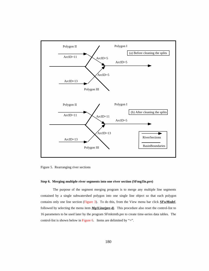
180
Polygon IPolygon II
Polygon III
ArcID=5
ArcID=5
ArcID=5ArcID=11
ArcID=13
(a) Before cleaning the splits
Polygon IPolygon II
Polygon III
ArcID=5
ArcID=13
ArcID=11ArcID=11
ArcID=13
(b) After cleaning the splits
RiverSections
BasinBoundaries
Figure 5. Rearranging river sections
Step 6. Merging multiple river segments into one river section (SFmg1ln.pre)
The purpose of the segment merging program is to merge any multiple line segments
contained by a single subwatershed polygon into one single line object so that each polygon
contains only one line section (Figure 3). To do this, from the View menu bar click SFwModel,
followed by selecting the menu item Mg1Line(pre-4). This procedure also reset the control-list to
16 parameters to be used later by the program SFmktmtb.pre to create time-series data tables. The
control-list is shown below in Figure 6. Items are delimited by “=”.

181
NGBASIN.ply=NGBASIN_=Grid_CodeNGRIVER.shp=NGRIVER_=Grid_CodeNGBASIN.lin=NGBASIN_dhtb.dbf=NGBASIN.ply=NGBASIN_=8,4=View1fflow.dbf=NGRIVER1.shp=Grid_code=9,2=View1gfvtb.dbf=NGBASIN.ply=NGBASIN_=14,11=View1headtb.dbf=NGBASIN.ply=NGBASIN_=8,2=View1pflow.dbf=NGBASIN.ply=Grid_code=8,3=View1pmptb.dbf=NGBASIN.ply=NGBASIN_=14,11=View1psurp.dbf=NGBASIN.ply=Grid_code=14,11=View1rchtb.dbf=NGBASIN.ply=NGBASIN_=14,11=View1respvt.dbf=NGRIVER1.shp=Grid_code=7,4=View1sprtb.dbf=NGBASIN.ply=NGBASIN_=8,3=View1tflow.dbf=NGRIVER1.shp=Grid_code=9,2=View1xfluxtb.dbf=NGBASIN.lin=NGBASIN_=14,11=View1yfluxtb.dbf=NGBASIN.lin=NGBASIN_=14,11=View1
Figure 6. Control-list set to the object-tag at the project level (16 parameters)
Step 7. Identifying the head and outlet sections on the river network (SFchkout.pre)
This procedure identifies the outlet (by setting ISOUTLET=1) and head (by setting
ISHEAD=1) sections on the river network. To do this, from the View menu bar click SFwModel,
followed by selecting the menu item ChkInOut(pre-5).
Step 8. Creating data structure to hold spatially-referenced time-series tables
Altogether 13 database tables are created to hold spatially-referenced time-series tables
(Figure 6). These time-series tables are used by both map-based surface and subsurface simulation
models. To perform this task, from the View menu bar click SFwModel, followed by selecting
menu item Crtmtb(pre-6). All the databases holding the spatially-referenced time-series tables
have the data structure shown in Figure 7.

182
Number Of Fields = Number Of Records In (AAT/PAT)Field Names="GC"+ValuesOfCover_ID in (AAT/PAT)
Time/Stage GC1 GC2 GC3 ..........
1
2
........
Rec
ordN
umbe
r=T
imeS
teps
Figure 7. Database Structure for spatially-referenced time-series data
Step 9. Creating other model supportive files
This procedure creates 8 files/coverages used by the model. These files are (1) dams.shp,
(2) flowchk.shp, flowdist.dbf, flowtime.dbf, optmass.dbf, optsrme.dbf, mflowfit.dbf, and
target.dbf. To start the procedure, from the View menu bar, click SFwModel followed by
selecting the menu item MkFVtbls(pre-7).
Step 10. Creating polygon/line objects for GFlowSim
This procedure appends the fields needed for the map-based groundwater simulation
model (GFlowSim) to the polygon (NGBASIN.ply) and line (NGBASIN.lin) coverages. To
perform the task, from the View menu bar, click GFwModel, and select the menu item
GFmdfld(pre-1).
Step 11. Setting up polygon coverage for GFlowSim
Click GFwModel, and select the menu item SetPlyFld(pre-2) to set up the polygon
coverage (NGBASIN.ply) for GFlowSim.
Step 12. Setting up boundary line coverage for GFlowSim
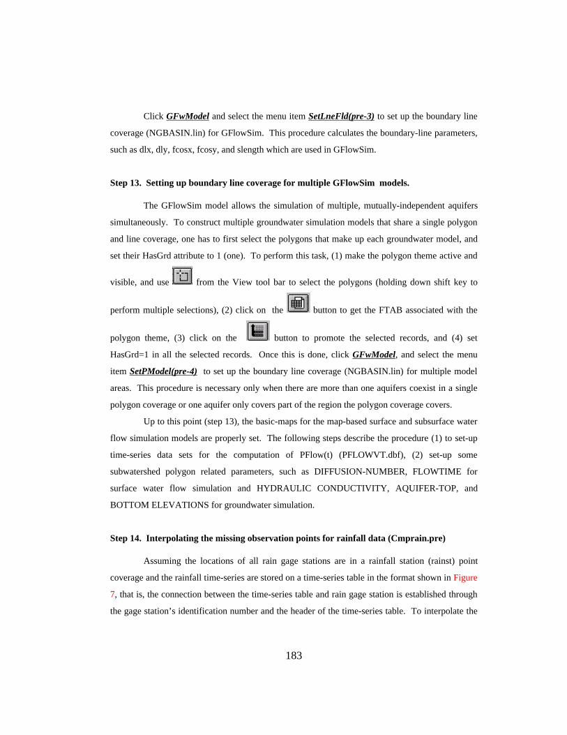
183
Click GFwModel and select the menu item SetLneFld(pre-3) to set up the boundary line
coverage (NGBASIN.lin) for GFlowSim. This procedure calculates the boundary-line parameters,
such as dlx, dly, fcosx, fcosy, and slength which are used in GFlowSim.
Step 13. Setting up boundary line coverage for multiple GFlowSim models.
The GFlowSim model allows the simulation of multiple, mutually-independent aquifers
simultaneously. To construct multiple groundwater simulation models that share a single polygon
and line coverage, one has to first select the polygons that make up each groundwater model, and
set their HasGrd attribute to 1 (one). To perform this task, (1) make the polygon theme active and
visible, and use from the View tool bar to select the polygons (holding down shift key to
perform multiple selections), (2) click on the button to get the FTAB associated with the
polygon theme, (3) click on the button to promote the selected records, and (4) set
HasGrd=1 in all the selected records. Once this is done, click GFwModel, and select the menu
item SetPModel(pre-4) to set up the boundary line coverage (NGBASIN.lin) for multiple model
areas. This procedure is necessary only when there are more than one aquifers coexist in a single
polygon coverage or one aquifer only covers part of the region the polygon coverage covers.
Up to this point (step 13), the basic-maps for the map-based surface and subsurface water
flow simulation models are properly set. The following steps describe the procedure (1) to set-up
time-series data sets for the computation of PFlow(t) (PFLOWVT.dbf), (2) set-up some
subwatershed polygon related parameters, such as DIFFUSION-NUMBER, FLOWTIME for
surface water flow simulation and HYDRAULIC CONDUCTIVITY, AQUIFER-TOP, and
BOTTOM ELEVATIONS for groundwater simulation.
Step 14. Interpolating the missing observation points for rainfall data (Cmprain.pre)
Assuming the locations of all rain gage stations are in a rainfall station (rainst) point
coverage and the rainfall time-series are stored on a time-series table in the format shown in Figure
7, that is, the connection between the time-series table and rain gage station is established through
the gage station’s identification number and the header of the time-series table. To interpolate the

184
missing rainfall data, click the tool and select the program CMPRAIN.PRE. (Some program
variables, such as ThmName, RainTbName, "RainId", may need to be modified to point at the
correct data sets before the program can be run). Because the procedure uses a squared-inverse-
distance scheme for the missing data point and all the distance are dynamically computed at the
run-time, running the interpolation program can be very time consuming if the rainfall data come
from a large set of rain gage stations with long observing periods. Therefore, it may be desirable
to cut the rainfall data to the simulation interval for rainfall interpolation.
Step 15. Interpolating the rainfall time-series to the center points of subwatersheds or cells
for soil-water-balance computation (cmpsurp.pre)
The purpose of this procedure is to interpolate the rainfall time-series (stored in a data
table in the format given in Figure 7) to the time-series defined on the center points of each
subwatershed to be used as water-surplus for PFlow(t) computation, or to the centers of the cells
used for soil-water balance computation. To activate the procedure, click the tool, select
the program CMPSURP.PRE, and follow the procedures provided by the pop-up menus. (Again,
some variables in CMPSURP.PRE may need to be modified to match the names of the data sets and
themes).
Step 15. Computing DiffNum, FlowTime for subwtershed polygons
If PFlow(t) is to be computed using a convolution procedure, then the parameters,
DiffNum, FlowTime of the subwatershed polygons need to be set. To compute the parameters
necessary to compute Flowtime and Diffnum, the program listed in Figure 8 written by Seann
Reed can be used (The program needs to be run under ARC/GRID using DemFil, DemFdr, and
DemShd as input grids (See Figure 2).
The program listed in Figure 8 produces the mean flow distance and standard deviation of
the distance for each polygon. Once this two parameters are computed, the DiffNum (Di) and
FlowTime can be computed using the following formula:

185
Di =σ i
2
2(li2 )
(1)
Ti = li/Vfact (2)
where, li = average flow length of polygon i (m),
σi = standard deviation of the flow length for polygon i (m),
Vfact = average overland flow velocity (m/s)
Both li and σi are stored in file length.dat by the procedure listed in Figure 8.
/*******************************************************/* Name: pac_par.aml/* Purpose: Determine the parameters necessary to calculate/* a "flowtime" and a "diffusion number"./******************************************************/** FOR THE CASE OF THE MISSION RIVER, THE ARGUMENTS
ARE:/* dem = demfil /* DEM/* sheds = missub /* Mask of watersheds/* fd = misfdns /* Flowdirection grid/*&args dem sheds/** SET VARIABLES FOR INPUT GRIDS&sv fd = misfdns&sv sheds = missubfl = flowlength ( %fd%, #, downstream )flmin = zonalmin ( %sheds%, fl, data )flsub = fl - flminlength.dat = zonalstats ( %sheds%, flsub, moment, data )
Figure 8. Code for polygon related parameter computation
2.2 THE MAPS OF THE SIMULATION MODEL
Figure 9 shows the view containing the themes upon which the simulation model is
constructed. The themes contained in the Niger-View and their functions are discussed below.

186
Figure 9. The view containing the base maps of the simulation model
Listed below are the coverages representing the base maps upon which the surface water
flow simulation model is constructed.
• NGRIVER.shp - An arc coverage representing the river network. This line coverage is
essential for the construction of the map-based surface water flow simulation model
(SFlowSim)
• NGBASIN.ply - A polygon coverage representing the subwatershed of the river basin for
surface water flow simulation model and representing cells for the groundwater
simulation model. This coverage is essential for the construction of both surface water
flow simulation model and groundwater flow simulation model.
• NGBASIN.lin - An arc coverage representing the boundary lines of subwatershed
polygons (NGBASIN.ply). This coverage is needed for the construction of the
groundwater simulation model (GFlowSim)

187
• Dams.shp - Point coverage representing locations of dams and reservoirs
• Flowchk.shp - Point coverage representing the locations where the flow interpolation
will be computed
The coverages that are essential for the map-based surface water flow simulation models
are NGRIVER.shp and NGBASIN.ply. The coverages essential for the map-based groundwater
simulation model are NGBASIN.ply and NGBASIN.lin. Dams.shp and flowchk.shp are needed if
these objects present. As Dams.shp, flowchk.shp and other non-essential model data files are
generated by the program SFMkFtab.pre from the pre-processor module, the coverages necessary
to construct base maps for the integrated surface and subsurface water flow simulation model are
(1) NGBASIN.ply, NGRIVER, and NGBASIN.lin.
2.3. THE MODEL’S GRAPHICAL USER INTERFACE
The graphical user interface of the simulation model (SFlowSim) is designed to provide
easy access to the simulation model and its related programs. A user can use these graphical
interfaces to activate the simulation model, modify the model conditions, add flow check points,
flow diversion points, or add dam/reservoir objects. This section describes the functions associated
with each user interface.
2.3.1. View Menu
Two menu sections, SFwModel and GFwModel have been added to the standard View
menu bar GUI provided by the ArcView. SFwModel menu runs the surface water flow simulation
model and its related programs while GFwModel menu runs the groundwater flow simulation
model and its related programs. Figure 10 shows the menu items contained in SFwModel and
GFwModel menu.
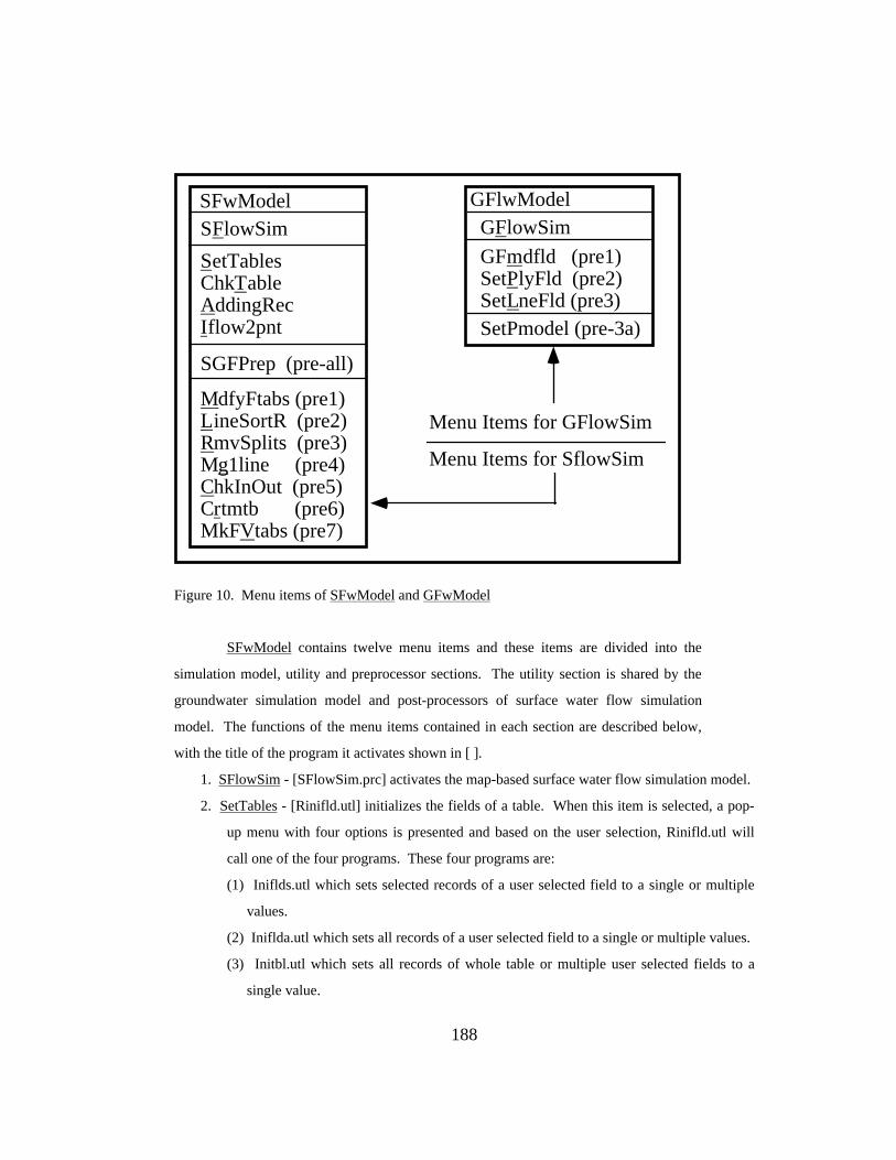
188
SFwModel
MdfyFtabs (pre1)LineSortR (pre2)RmvSplits (pre3)Mg1line (pre4)ChkInOut (pre5)Crtmtb (pre6)MkFVtabs (pre7)
SFlowSim
SetTablesChkTableAddingRecIflow2pnt
GFlwModelGFlowSim
GFmdfld (pre1)SetPlyFld (pre2)SetLneFld (pre3)
Menu Items for SflowSim
Menu Items for GFlowSim
SetPmodel (pre-3a)
SGFPrep (pre-all)
Figure 10. Menu items of SFwModel and GFwModel
SFwModel contains twelve menu items and these items are divided into the
simulation model, utility and preprocessor sections. The utility section is shared by the
groundwater simulation model and post-processors of surface water flow simulation
model. The functions of the menu items contained in each section are described below,
with the title of the program it activates shown in [ ].
1. SFlowSim - [SFlowSim.prc] activates the map-based surface water flow simulation model.
2. SetTables - [Rinifld.utl] initializes the fields of a table. When this item is selected, a pop-
up menu with four options is presented and based on the user selection, Rinifld.utl will
call one of the four programs. These four programs are:
(1) Iniflds.utl which sets selected records of a user selected field to a single or multiple
values.
(2) Iniflda.utl which sets all records of a user selected field to a single or multiple values.
(3) Initbl.utl which sets all records of whole table or multiple user selected fields to a
single value.

189
(4) Inifdfd.utl which initializes a field of a table with the values of a field of another table
based on the user selected key fields on both tables. These two key fields can have
different field name, but their values need to have a one-to-one relation.
3. ChkTable - [Rchktbl.utl] displays the data structure of a value attribute table or a feature
attribute table. When this item is selected, a pop-up menu with two options is presented
and based on the user selection, the program [Rchktbl.utl] will call one of the two
programs. These programs are:
(1) [Chktbl.utl] which checks and displays the data structure of a value attribute table.
(2) [Chkftab.utl] which checks and displays the data structure and the shape type of a
feature attribute table.
4. AddingRec - [tbaddrec.utl] appends a user specified number of records to a time-series
table.
5. Iflow2pnt - [Iflw2pnt.utl] interpolates flow rates to the locations given by a point
coverage.
6. SGFPrep (pre-all) [preproc.pre] processes all the pre-processing procedure for both
surface and subsurface water flow simulation models.
7. MdfyFtabs (pre-1) - [SFmdfld.pre] appends fields to line/polygon attribute tables to create
river and river basin objects.
8. LineSortR (pre-2) - [SFsortR.pre] sorts nodes and vertices of a river line coverage to create
the river network. After sorting, the direction of From-Node to To-Node of a river
section always points in the downstream direction and the vertices with index 0 is at the
From-Node of the arc.
9. RmvSplits (pre-3) - [SFsplit.pre] cleans the splits of a river network so that “Y” shaped
streams do not occur within a subwatershed.
10. Mg1line (pre-4) - [SFmg1ln.pre] merges multiple segments contained by a single
subwatershed (polygon) into one single river section so that the relation between river
section and subwatershed polygon is One-to-One.
11. ChkInOut (pre-5) - [SFchkout.pre] identifies head sections and outlet sections of the river
network. The head sections are defined as the river sections with no other river sections
that flow into them and the outlet section is defined as the river section that discharges to
no other river sections but out of the river basin.

190
12. Crtmtb [pre-6] - [SFmktmtb.pre ->wrtmfile.pre] creates time-series tables, e.g., FFlowTb,
TFlowTb, PFlowTb, etc., for the simulation model.
13. MkFvtabs [pre-7] - [MkFtab.pre] creates dams.shp, flowchk.shp and other data tables for
the simulation model.
The five pre-processor programs (pre-1 to pre-5) need to be run in the same sequence as they are
presented in the SFwModel ViewMenu.
GFwModel contains 5 menu items and these items are divided into simulation mode and
preprocessor sections. The functions of the menu items are described below, with the title of the
program it activates put in [ ].
1. GFlowSim - [GFlowSim.prc] activates the map-based groundwater simulation model.
2. GFmdfld (pre-1) - [GFmdfld.pre] appends fields to polygon and polygon-boundary-line
attribute tables to make cell and cell boundary objects for the map-based groundwater
simulation model.
3. Setplyfld (pre-2) - [GFplyfld.pre] computes and fills in the states of the existing cell objects
for the groundwater simulation model.
4. Setlnefld (pre-3) - [GFlnefld.pre] computes and fills in the states of the cell-boundary-line
objects for the groundwater simulation model.
5. SetPmodel (pre-4) - [GFlnsfld.pre] constructs multiple groundwater simulation models.
Before running the program, one has to select all the polygons in the model-regions and
set their attribute: HasGrd=1 (has-ground = one).
All the pre-processor programs should be run only once to set up the map-based models unless the
base maps of the model are modified.
2.3.2. View Button Bar
Four buttons are added to the standard View button bar GUI provided by the ArcView.
The functions and programs associated with these buttons are explained below (immediately
following each icon is the icon name given by ArcView’s icon manager).
- PennantGreen, interpolates flow rates to the points given by FlowChk.shp coverage
[SFsegmt.pst].

191
- Pen, writes selected or all the scripts contained in the project’s SEd to a designated
location on a disk [wrtfiles.utl].
- Cut, cuts selected portion of the active coverages and sends them to a new view to
create a sub-model for either detailed study of the region or for model parameter fitting
[clipmdl.utl].
- Dog, runs interactive optimization programs to search for the parameters that give the
best fit between observed-flow-time-series and simulation model generated flow-time-
series[Optimize.ave]. The best fit is defined either by least sum of square errors or least
sum of mass differences. When running the model, at least one coverage theme must be
active and at least one feature of the coverage has to be selected, because the parameters to
be fitted are those of the active coverages and selected features.
- STAR, sets up the control list (ctrllist) or model’s time dimension (model interval)
[setctrl.utl] & [setmctrl.utl - set-time-ctrl].
2.3.3. View Tool Bar
Four buttons are added to the standard view button bar GUI provided by the ArcView.
The functions and programs associated with these buttons are explained below.
- Execute, runs all the programs available to the Script Editor (SEd) of the project
[Main.utl - activated by apply event]. When the tool is selected, the program, Main.utl is
loaded and activated when the mouse is clicked in the cursor sensitive area of the active
view. The last program run by the Main.utl is the default program to be run again. If the
user wants to run other programs, select NO option, and a pop-up menu will appear with a
list of programs for the user to choose. The selected program will then run with the cursor
position taken into consideration.
- PennantRed (red color), creates dam, reservoir, flow diversion, or flow-check point
objects on a location selected by the program user. Programs associated with click and
apply events are listed below.

192
CLICK - [SFclsset.pst] provides options for a user to select what kind of object (dam,
flowchk, or flow-diversion points) to create, and if the user would like to start with
new sets or append more objects to the existing set. The program passes the user
selection through the tool’s object-tag to [SFRaddpt.pst].
APPLY - [SFRaddpt.pst] runs one of the three programs, [SFaddpt.pst], [SFDFlow.pst],
or [SFaddDam.pst], depending on the value of the object-tag (representing the user
selection) passed on to it from [SFclsset.pst].
[SFaddpt.pst] - creates flow check points at user specified locations and adds them
to the FLOWCHK.SHP coverage. The flow rates at the flow check points will
later be computed using the program [SFsegmt.pst] activated by the
button (green color) on the View-Button-Bar.
[SFDFlow.pst] - creates a flow diversion object at a user specified location on a
river. For now, only one diversion flow rate is allowed at one location, later
on, a diversion flow rate time-series can be associated with the diversion
object.
[SFaddDam.pst] - creates a dam/reservoir object at a user specified location on a
river, and the time-series data table associated with the dam object so that each
time step, the simulation results of the dam operation can be recorded.
- Icon12, plots either the longitudinal flow profile along a user selected river or a flow
time-series (PFlow(t), FFlow(t), TFlow(t), or SurpF(t)), at a user selected location.
Programs associated with click and apply events are listed below.
CLICK - [SFsetplt.pst] provides options for a user to select which type of flow curves to
plot and passes on the selection through the tool’s object-tag to [SFRplt.pst].
APPLY - [SFRplt.pst] runs one of the three programs, [SFtrplt.pst], [SFtmplt.pst], or
[Sfptflow.pst] based on the value of the object-tag passed on to it from
[SFsetplt.pst].
[SFtrplt.pst] - plots the longitudinal flow profile along a selected river.
[SFtmplt.pst] - plots the flow time-series at a user selected location.
[Sfptflow.pst] - plots the interpolated flow time-series at a user designated location

193
- AlingBottom, plots flow vectors on groundwater simulation cell’s boundaries or plots
time-series of head(t), dh(t), spr(t), pmp(t), etc., of a cell at a user selected location.
Programs associated with click and apply events are described below.
CLICK - [GFsetplt.pst] provides options for a user to select which type of flow curves to
plot and passes on the selection through the tool’s object-tag to [GFRplot.pst]
APPLY - [GFRplot.pst] runs one of the two programs, [GFptflx.pst] or [GFpthead.pst],
based on the value of the object-tag passed on to it from [GFsetplt.pst].
[GFptflx.pst] - plots flux, water level distributions, or both for the groundwater
flow simulation model. Under steady state, it plots flux, and water level
distributions based on the final results of simulation run and under steady state,
it plots the above values at a user designated time step.
[GFpthead.pst] - plots water level (head(t)), spring flow (spr(t)), water level
variations (dh(t)) at a user selected location.
2.4. MODEL PROGRAMS
The map-based surface water flow simulation model contains a total of 46 programs.
Some of these programs are essential programs for model construction and model simulation and
some of these programs are merely written to speed up routine spatial data processing. This
section describes these programs and their functions. The number in the bracket following the
program indicates the number of lines of the program code.
1. chkctrl.utl [14] - checks the model’s control set. Control set contains the information of
coverage name, key-field-name, grid-code, and model time-steps.
2. chkftab.utl[34] - checks the data structures and shape type of a feature attribute table.
3. chktbl.utl[35] - checks the data structures of a value attribute table.
4. clipmdl.utl[184] - clips off a selected portion of the active coverage and sends it to a new
view to create a clipped model for either detailed study of the region or for model
parameter fitting
5. cmprain.pre[118] - fills in missing rainfall time-series data at a point by interpolating the
rainfall time-series from other rain-gage stations

194
6. cmpsurp.pre[152] - estimates moisture surplus for each subwatershed from the rainfall
time-series data defined on the rain-gage stations in the region.
7. convert.utl [587] - converts parameter set between spatial features on which they are
defined.
8. Damrt.ave[208] - simulates dam/reservoir operation. This program is called by
SFlowSim.prc when HASDAM attribute of a river line object is non-zero.
9. GFcntpnt.utl[132] - computes the center location of each arc on a selected line coverage
and creates a point coverage showing all the central points based on the computation
results. The program also computes and creates a line coverage showing the arcs normal
to the original line coverage with each normal vector originates at the center of each line
on the original line coverage.
10. GFlnfld.pre[291] - computes and fills in the states of each boundary lines of the existing
cells for the groundwater simulation model.
11. GFlnsfld.pre[232] - computes and fills in the states of each boundary lines when the
groundwater model does not cover the same area of the surface water flow simulation
model.
12. GFlowSim.prc[916] - simulates groundwater flow. This is the main program of the
map-based groundwater flow simulation model.
13. GFmdfld.pre[79] - appends fields to the standard polygon/arc coverage to create cells
and cell boundary line objects for the map-based groundwater simulation model.
14. GFplyfld.pre[51] - computes and fills in the states of the existing cell objects for the
groundwater simulation model.
15. GFptflx.pst[266] - plots flux on the cell boundaries, water levels on the cells or both for
a user selected simulation time step or of final results of the groundwater simulation
model. This is a post processor program of GFlowSim.
16. GFpthead.pst[141] - plots time-series of water levels (head(t), dh(t), pmp(t)) of a user
selected location. This is a post processor program of GFlowSim.
17. GFRplot.pst[36] - runs either [GFpthead.pst] or [GFptflx.pst] based on the user’s
selection.

195
18. GFsetplt.pst[17] - provides user with options of plotting groundwater flow time-series
of a location or groundwater flux/water level of a designated time step and passed user’s
selection to [GFRplot.pst]
19. IDextply.pst[88] - identifies the external boundaries of the groundwater simulation
model. This program is used mainly on the clipped portion of the river basin to form a
clipped-groundwater simulation model.
20. Iflw2pnt.utl[341] - interpolates flow rates to the points given by a point coverage.
21. Inifdfd.utl[58] - initializes a field of a table with the values of a field of another table
based on the user selected key fields on both tables. These two key fields can have
different field name, but their values need to have a one-to-one relation.
22. Iniflda.utl[159] - sets all records of a user selected field to single or multiple values.
23. Iniflds.utl[82] - sets selected records of a user selected field to single or multiple values.
24. Initbl.utl[134] - sets all records of whole table or multiple user selected fields to a single
value.
25. Main.utl[46] - runs a user selected program.
26. MKarrow.utl[61] - makes an arrow head on a line coverage. This program is
downloaded from ESRI user network and has been slightly modified.
27. mkftab.pre[239] - creates dams.shp, flowchk.shp and data tables (optmass.dbf,
optsrme.dbf, target.dbf, flowdist.dbf, and flowtime.dbf) for the simulation model.
28. Optimize.ave[855] - this is a directional optimization program used to search for the
parameters that give the best fit between observed-flow-time-series and simulation
model generated flow-time-series at a user-specified location. The best fit is given by
the simulated flow time-series that has SMD=0 and min.RMSE. When running the
model, at least one coverage theme must be active and at least one feature of the
coverage has to be selected, because the parameters to be fitted are those of selected
features on the active coverages (Themes). This program calls SFlowSim.prc to
simulate the surface water flow for each parameter change.
29. preproc.pre [16] - calls other pre-processing programs of surface and subsurface water
flow simulation models for model setup.
30. Rchktbl.utl[25] - Runs either [chkftab.utl] or [chktab.utl] based on the user’s selection.

196
31. Rinifld.utl[31] - Runs one of the four programs, [Iniflda.utl], [Iniflds.utl], [Initbl.utl], or
[Inifdfd.utl] based on the user’s choice.
32. setctrl.utl [219] - creates model control set, which contains cover-name, cover-id, grid-
code, and time-steps.
33. setmctrl.utl [149] - resets model’s time-step control.
34. SFAdddam.pst[270] - creates a dam/reservoir object and puts it in the location
designated by the user. The program also creates a time-series table associated with the
dam object to record the simulation results of dam operation.
35. SFaddpt.pst[54] - creates a flow check point and puts it to a location designated by the
user.
36. SFchklin.utl[85] - retrieves all the vertex points used to form a line and puts the points
shape into flowchk.shp file.
37. SFchkout.pre[156] - searches and identifies the head sections and outlet sections of a
river basin.
38. SFclsset.pst[131] - gets the user’s choice regarding the type point objects, dam, flow-
check, or flow-diversion, to create and passes on the user’s selection to [SFRaddpt.pst].
39. SFDflow.pst[52] - creates a flow diversion points and puts a mark on the map to
indicate its location.
40. SFdslv.utl[186] - assigns single cell ploygons with appropriate Grid-Codes so that they
can be dissolved.
41. SFlowSim.prc[1244] - simulates surface water flows on a river network based on the
local flow time-series defined on the subwatershed polygons. This is the major program
of this map-based surface water flow simulation model. This model can be activated by
[Main.utl] from a tool-bar, SFlowSim on the SFwModel view menu, or called by
[Optimize.ave], the interactive optimization program. SFlowSim.prc can detect from
which source it is activated and act accordingly. For example, when it is activated by
from the View tool bar, the program will takes the cursor’s location into consideration,
and as a result, it provides the user with choices of either simulating the whole river
basin or the portion of the river basin that is above the user selected point (cursor
location). When it is activated by from the view-menu, it can only simulate the river

197
basin. When it is called by the optimization program, it skips over all the codes that
requires user interaction so that the simulation program can run uninterruptedly.
42. SFmdfld.pre[160] - appends fields to attribute tables of the arc/polygon coverage
created by the river delineation procedure to create river and watershed objects.
43. SFmg1ln.pre[361] - merges multiple segments contained by a single subwatershed
(polygon) into one single river section so that the relation between river section and
subwatershed polygon is one-to-one [SFmg1ln.pre].
44. [Sfptflow.pst] - plots the interpolated flow time-series at a user designated location.
45. SFRaddpt.pst[39] runs one of the three programs, [SFaddpt.pst], [SFDFlow.pst], or
[SFaddDam.pst], based on the user’s selection.
46. SFRplot.pst[36] - runs one of the two programs, [GFptflx.pst] or [GFpthead.pst], based
on the value of the object-tag passed on to it from [GFsetplt.pst].
47. SFSegmt.pst[333] - linearly interpolates the flow rates to the user selected location.
48. SFsetplt.pst[17] - gets the choice from a user on which type of curve to plot and pass on
the selection to [SFRplot.pst] through the form of object-tag.
49. SFsortr.pre[531] - sorts nodes and vertices of river line coverage to create the river
network [SFsortR.pre]. After sorting, the direction of From-Node to To-Node of a river
section is always pointing in the downstream direction and the vertex with index 0 is at
the From-Node of the arc.
50. SFsp2pf.121[84] - computes local generated flow based on the moisture surplus defined
on the subwatershed polygons.
51. SFsplit.pre[532] - cleans the splits of the river sections so that “Y” shaped streams do
not occur within a subwatershed [SFsplit.pre].
52. SFthmplt.pst[97] - calls the program wrtmfile.pre based on the parameters provided by
the control file, sfdbfs.ctl to create time-series data tables.
53. SFtmplt.pst[134] - plots time-series of a selected attribute at a selected location.
54. SFtrplt.pst[402] - plots flow rate changes along a user selected river.
55. tbaddrec.utl[69] - appends records to a time-series data table. The number of records is
given by the user.
56. tbsvgd.utl[28] - closes all the open value attribute tables (VTab) and feature attribute
tables (Ftab).

198
57. Wrtfiles.utl[85] - writes either selected or all the scripts contained in the project’s SEd
to a designated location of a disk
58. wrtmfile.pre[82] - called by SFmktmtb.pre to write a program that create the template
for a time-series database table.
59. Wrtprogs.utl[71] - writes an Avenue code that can be later run to create the template of
a time-series database table.
3. Performing Tasks under SFlowSim/GFlowSim
This section gives a brief description of the procedures to perform tasks using SFlowSim,
the map-based surface water flow simulation model.
3.1. SURFACE WATER FLOW SIMULATION
The map-based surface water flow simulation model is designed to simulate surface water
flow runoff based on the excess precipitation defined on the subwatersheds of a river basin.
Running the simulation model generates three flow time-series: PFlow(t) associated with a
subwatershed polygon representing the flow contribution of the polygon, FFlow(t) and TFlow(t)
associated with the From-Node and To-Node of a river line representing the flow rates on the river
line at these two locations. Two procedures can be used to run the simulation model.
Procedure (1): while model-map view is an active document, do the following: from
View menu bar, SFlwModel -> SFlowSim
Procedure (2): while model-map view is an active document, click from the View
tool bar, followed by clicking at a river line, selecting SFlowSim.prc from the program list
presented, and following the instructions. Using procedure (2), you can simulate either the portion
of the river basin above the river line selected or the whole river basin, while using procedure (1)
you can only simulate the whole river basin.
Regardless of which procedure is used to run the simulation model, a user will be
presented with a multiple input table containing the model control parameters. Under most cases,
the default value can be used to run the model unless it is desired otherwise. The meanings of the
parameters are described below:

199
(1) Optimization=0, indicates if the run is for optimization (value 1) or for simulation
only (value 0)
(2) CalPflow=0, indicates if PFlow will be re-computed [value 1], or not [value 0]
(3) Nresp=12, number of steps in polygon response function (SurpF(t) -> PFlow(t)),
Nresp=0, indicating PFlow(t) is estimated from SurpF(t) without using a response
function.
(4) IniTmStep=1, Starting time step
(5) EndTmStep=365, Ending time step
(6) ToSub=0.1, the fraction of surplus that goes to groundwater, 0<=ToSub<=1
(7) Muskingum=0, indicates if Muskingum river routing will be considered (=1) or not
(=0)
(8) Pltply=1, indicating polygons will be highlighted during simulation.
The value following the equal sign of each parameter indicates the program default.
3.2. CREATING DAM/FLOWCHK/DIVERSION OBJECTS
The simulation model can simulate the effect of dams and flow diversions on the river
flow. The simulation model can also interpolate the flow rate to any user selected point (flowchk)
on a river line. The procedure used to create a Dam/FlowChk/Diversion object and add it to the
map is:
Click (RedFlag) from the View tool bar, select the type of the object to be added,
and then click on a location on the stream network where you would like to have the object
inserted. After the selection, the user is prompted to select whether to start a new set of the object
or append to the existing set. If starting a new set is selected, then all the objects of the selected
class will be cleaned from the system. This is also the correct method if one wants to erase the
existing object sets.
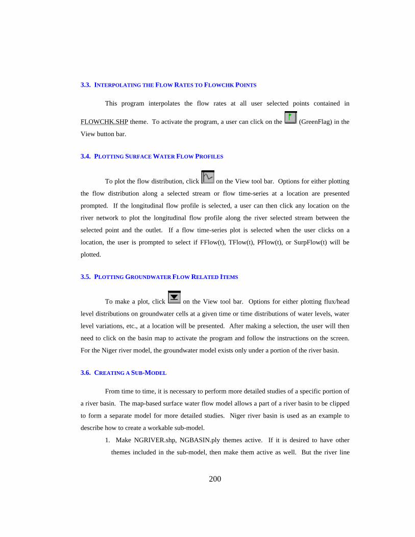
200
3.3. INTERPOLATING THE FLOW RATES TO FLOWCHK POINTS
This program interpolates the flow rates at all user selected points contained in
FLOWCHK.SHP theme. To activate the program, a user can click on the (GreenFlag) in the
View button bar.
3.4. PLOTTING SURFACE WATER FLOW PROFILES
To plot the flow distribution, click on the View tool bar. Options for either plotting
the flow distribution along a selected stream or flow time-series at a location are presented
prompted. If the longitudinal flow profile is selected, a user can then click any location on the
river network to plot the longitudinal flow profile along the river selected stream between the
selected point and the outlet. If a flow time-series plot is selected when the user clicks on a
location, the user is prompted to select if FFlow(t), TFlow(t), PFlow(t), or SurpFlow(t) will be
plotted.
3.5. PLOTTING GROUNDWATER FLOW RELATED ITEMS
To make a plot, click on the View tool bar. Options for either plotting flux/head
level distributions on groundwater cells at a given time or time distributions of water levels, water
level variations, etc., at a location will be presented. After making a selection, the user will then
need to click on the basin map to activate the program and follow the instructions on the screen.
For the Niger river model, the groundwater model exists only under a portion of the river basin.
3.6. CREATING A SUB-MODEL
From time to time, it is necessary to perform more detailed studies of a specific portion of
a river basin. The map-based surface water flow model allows a part of a river basin to be clipped
to form a separate model for more detailed studies. Niger river basin is used as an example to
describe how to create a workable sub-model.
1. Make NGRIVER.shp, NGBASIN.ply themes active. If it is desired to have other
themes included in the sub-model, then make them active as well. But the river line

201
theme (NGRIVER.shp) and subwatershed polygon theme (NGBASIN.shp) are the
essential themes and they have to be included to create a sub-model.
2. Select the river lines graphically from NGRIVER.shp theme and NGBASIN.ply theme
by using the selection tool in View tool bar. Hold down the shift key to perform
multiple selections.
3. Click on the View button bar. The program will prompt for the location to put
the shape files holding the selected features of the selected themes (NGRIVER.shp,
NGBASIN.ply). In most cases, a user can take the default prompted by the program.
When prompted with the destination View to which the clipped themes will be added,
the user should select NewView. The program will detect all the source arcs on the
sub-model. The sources are defined as those river lines that require FFlow(t) supplied
by the user or provided from the “base-model” simulations.
4. Up to this point, a sub-model that contains the selected portion of the selected themes
is created. All the surface model simulation programs can be run following exactly the
same procedures as those for the “base-model”. One of the purpose of creating sub-
model is to run the interactive optimization program that is discussed below.
3.7. MODEL PARAMETER OPTIMIZATION (MODEL CALIBRATION)
The optimization model is created to search for the model parameters that produce flow
time-series that best fit the historically observed time-series in terms of sum of root mean square
errors (RMSE) and mass conservation (SMD). The results of the optimization are shown in four
tables, optmass.dbf, optsrme.dbf, mfitflow.dbf and target.dbf, and four charts, optrmse.cht,
optmass.cht, tarteg.cht, and mfitflow.cht. Optmass.cht, created from optmass.dbf, gives the
changes of SMD as each optimization parameter changes. Optsrme.cht, created from optrmse.dbf,
gives the changes of RMSE as each optimization parameter changes. Target.cht, created from
target.dbf, gives the comparison between the observed and simulated river flow time-series.
Mfitflow.cht, created from Mfitflow.dbf, gives the comparison of observed and simulated monthly
average flows.
1. Create a sub-model following the procedures described in Section 3.6.
2. Initialize the Target field of Target.dbf table using :

202
SFlwModel -> SetTables ->FillOneFieldWithAnother (option3)
The program, FillOneFieldWithAnother requires a user to identify a target table whose
field is to be set, a source table where the source data are stored, a target field and a key
field of the target and source tables. The key fields for target and source tables do not
need to have the same name, but need to have the same data structure and unique one-
to-one relation.
3. Make the themes whose parameters are to be optimized active. For example, if the
parameters of NGRIVER.shp are to be optimized, then NGRIVER.shp theme has to be
active.
4. Select the features (river lines or subwatershed) whose parameters are to be optimized
using ViewFeatureSelectTool, because the optimization is only applied to the selected
features (records) of the active themes.
5. Click on the View button bar to start the optimization program, and follow the
instructions prompted by the program. The optimization can be controlled by a
control file (optctrl.ctl). A sample control file is created by the program
SFmkFtab.pre activated by SFVtbls from under SFwModel menu. The files can be
modified to suit a specific need. If no sample control file is available, then select
CANCEL button when prompted for the control file name and follow the procedure
provided by the optimization program to create a new control file.
For each parameter to be optimized, the program requires a user to provide the upper
and lower bounds and optType. optType equals either 1, indicating that the
parameter goes to minimize RMSE or 0, indicating that the parameter goes to make
SMD=0.
3.8. MAP-BASED GROUNDWATER MODEL
The map-based groundwater model (GFlowSim) is created to account for groundwater
flows in cooperation with the map-based surface water flow simulation model (SFlowSim). The
groundwater model usually uses the same subwatersheds as its cells and cell boundaries. The
groundwater model can cover the same area of the whole river basin or several separate
groundwater models can coexist under one single large river basin to simulate separate

203
groundwater systems. For the Niger River Basin Model presented, only one groundwater model is
created to simulate the Iullemeden aquifer system. The region that the groundwater model covers
can be seen by making NGBASIN.lin active and querying with the condition of [ Hasgrd=1 and
Isbnd=1]. The procedure to run the groundwater model is: (from View menu bar)
GFlwModel->GFlowSim and follow the instructions provided by the program.
3.9. WRITING SCRIPTS CONTAINED IN THE PROJECT TO DISK
This program is written to facilitate writing all or selected script programs to a designated
location at a computer disk. To activate the program, click on the View button bar and follow
the instructions on the screen.
3.10. CREATING TIME SERIES DATABASE TEMPLATE
This program [Wrtprogs.utl] is written to create the template (class) of a time-series
database. To run the program, click on the View tool bar followed by clicking at the View
window. Select [Wrtprogs.utl] as the running program from the program list provided. Then
select the theme that the time-series data is associated with and the key field that contains unique
feature ID of the theme e.g. Cover_, or Cover_ID. The program will then write another program
name [Atmp.ave] and running program [Atmp.ave] will create the time-series database template
needed.
To create all the standard time-series data tables, refering to step 8 above for a proper
procedure.
3.11. SETTING UP MODEL’S CONTROL L IST
To setup the model’s control list, click on the - STAR button and follow the
instructions provided by the program.

204
3.12. RUNNING THE GROUNDWATER SIMULATION MODEL
The procedure to simulate groundwater flow with GFlowSim is, from View menu bar,
GFwModel -> GFlowSim . After the program starts, you will be presented with a multiple input
table containing the model control parameters. These parameters are described below:
(1) FluxPlot=100, A proportion used to scale the flux value so that the plot fits the
screen.
(2) BndFact=1.12, A fraction number accounting for effects of boundaries
(3) Sctrl=0.003, Storativity adjusting factor
(4) YesColor=5, plot the flux and water level as simulation proceeds; =0, do not plot.
(5) Pmodel=true, indicating there are more than one groundwater models running
simultaneously, Pmodel=false, indicating the model covers the whole study area.
(6) IsSteady=true, simulate steady state, =False, simulate unsteady state.
3.13. OTHER PROGRAMS
This map-based simulation model also provides utility programs to perform various
simulation model related tasks. These tasks include checking the data structure, field types of a
value attribute table or feature attribute table, disintegrating a line into points, appending records to
an existing database table, and flux line integration. More information about the utility programs
can be found in section two of this document.

205
Appendix II. The Spatially Referenced Time-Series Data Tables
TimeTblName Field SpFeature Model StateName KeyFieldDHTB.DBF (8.4) BasinPoly GFlow Dh(t) Cov# or Cov_FFLOW.DBF (8.2) RiverLine SFlow FFlow(t) Grid-Code or Grie_CodeGFVTB.DBF (14.11) BasinPoly GFlow DeltV(t) Cov# or Cov_HEADTB.DBF (8.2) BasinPoly GFlow Head(t) Cov# or Cov_PFLOW.DBF (8.3) BasinPoly SFlow PFlow(t) Grid-Code or Grie_CodePMPTB.DBF (8.3) BasinPoly GFlow Pump(t) Cov# or Cov_PSURP.DBF (14.11) BasinPoly SFlow PSurp(t) Grid-Code or Grie_CodeRCHTB.DBF (14.11) BasinPoly S-GFlow Rech(t) Cov# or Cov_RESPVT.DBF (7.4) RiverLine SFlow Resp(t) Grid-Code or Grie_CodeSPRTB.DBF (8.3) BasinPoly S-GFlow Spring(t) Cov# or Cov_TFLOW.DBF (8.2) RiverLine SFlow TFlow(t) Grid-Code or Grie_CodeXFLUXTB.DBF (8.3) BasinLine GFlow X-Flux(t) Cov# or Cov_YFLUXTB.DBF (8.3) BasinLine GFlow Y-Flux(t) Cov# or Cov_

206
Bibliography
Allard M. J., Hans A. M., Chris M., and Carlos R. (1994). Introduction to the Useof GIS for Practical Hydrology, UNESCO International HydrologicalProgramme, International Institute for Aerospace Survey and EarthSciences (ITC), p21.
Anderson, M.P. and Woessner W.W., (1992). Applied Groundwater Modeling :Simulation of Flow and Advective Transport, Academic Press Inc., SanDiego, CA.
Becker, E.B., Carey, G.F., and Oden, J.T., (1981). Finite Elements - Anintroduction, Volume I, Prentice-Hall, Inc., Englewood Cliffs, NJ.
Celia, M.A., and Gray, W.G., (1992). Numerical Methods for DifferentialEquations - Fundamental Concepts for Scientific and EngineeringApplications, Prentice Hall, Englewood Cliffs, NJ.
Cheney, W. and Kincaid, D. (1980). Numerical Mathematics and Computing,Brooks/Cole Publishing Company, Monterey, CA.
Chow, V.T., Maidment, D.R., Mays, L.W., (1987). Applied Hydrology, Mcgraw-Hill Book Company.
Cunge, J.A., (1969). “On the Subject of a Flood Propagation computationMethod (Muskingum Method),” J. Hydraul. Res., Vol. 7, No. 2, pp205-230.
Desai, C.T., (1979). Elementary Finite Element Method, Prentice Hall,Englewood Cliffs, NJ.
DeVantier, B.A., and Feldman, A.D. (1993). "Review of GIS Applications inHydrologic Modeling", Journal of Water Resources Planning andManagement, 119(2), pp246-261.
Djokic, D., Beavers, M.A., and Deshakulakarni, C.K. (1994). "ARC/HEC2: anARC/INFO - HEC-2 interface", Proceedings of the 21st AnnualConference on Water Policy and Management: Solving the Problems.

207
Domenico P.A., and Schwartz, F.W., (1990). Physical and Chemical Hydrology,John Wiley & Sons, NY.
Eckel, B. (1993). C++ Inside & Out, Osborne McGraw-Hill, CA.
ESRI, (1992). Cell-based Modeling with GRID 6.1, Supplement-Hydrologic anddistance modeling tools, ESRI, Redlands, CA.
ESRI, (1992). ARC/INFO Data Model, Concepts, & Key Terms, ESRI,Redlands, CA
Goldberg, A. (1983). Smalltalk-80: The Interactive Programming Environment,Addison-Wesley, NY.
Guerre, A. (1995). “GIS Hydrology for Africa - Bassin test du fleuve Niger,Report de mission (1-7 September, 1995).” Food and AgricultureOrganization (FAO).
Gunther, B. (1994) Object-Oriented Programming with Prototypes, Springer-Verlag, Berlin.
Huyakorn, P., and Pinder, G.F., (1983). Computational Methods in SubsurfaceFlow, Academic Press, NY.
Kuo, C.Y. (Edited by). (1993). Engineering Hydrology, American Society ofCivil Engineers, pp365-368, pp545-574, pp677-701.
Leipnik, M.R., Kemp, K.K., and Loaiciga, H.A. (1993). "Implementation of GISfor water resources planning and management", Journal of WaterResources Planning and Management vol. 119(2), pp184-205.
Linsley, R.K., Jr., Kohler, M.A., and Paulhus, J.L.H., (1982). Hydrology forEngineers, McGraw-Hill Book Company, NY.
Loucks, D.P., Stedinger, J.R., and Haith, D.A., (1981). Water Resources Planningand Analysis, Pretice-Hall, Inc., Englewood Cliffs, NJ.
Maidment, D.R., (1993). Developing a Watershed Data Structure, (A Reportprepared for the Hydrologic Engineering Center, US Army Corps ofEngineers, Davis, CA.).

208
Maidment, D.R., (1994). Hydrologic Modeling Using ARC/INFO, SeminarPresented at the 14th Annual ESRI User Conference, Palm Springs, CA.
Maidment, D.R., (Edited by) (1992). Handbook of Hydrology, McGRAW-HILL,INC., pp 10.7-10.13.
McCarthy, G.T., (1938). “The Unit Hydrograph and Flood Routing,” Conf. NothAtlantic Div., U.S. Corps of Engineers, New London, Conn.
McDonald, M.G., and Harbaugh, A.W., (1988) A Modular Three-DimensionalFinite-Difference Ground-Water Flow Model, USGS Open-File Report83-875. Chapter 11.
McKinney, D.C., and Tsai, H.L., (1996). “Multigrid Methods in a GIS Grid-CellBased Modeling Environment”, J. Computing in Civil Engineering,ASCE, 10(1), 25-30
Mintz, Y., and Serafini, Y.V., (1992). "A Global Monthly Climatology of SoilMoisture and Water Balance", Climate Dynamics, 8, 13-27.
Olivera, F. and Maidment, D.R., (1996). "Runoff Computation Using SpatiallyDistributed Terrain Parameters", accepted for publication in theProceedings of the ASCE North American Water and EnvironmentCongress '96, Anaheim, CA.
Pinder, G.F., (1973). "A Galerkin Finite-Element Simulation of GroundwaterContamination on Long Island", Water Resources Research, v.9, No. 6,pp1657-1664, NY.
Pinder, G.F., and Gray, W.G., (1977). Finite Element Simulation in Surface andSubsurface Hydrology, Academic Press, NY.
Press, W.H., et al., (1992). Numerical Resipes in C, Second Edition, CambridgeUniversity Press, pp353-354, pp394-405.
Razavi, A.H. (1995). ArcView Developer's Guide, OnWord Press.
Remson, I., Honrberger, G.M., and Molz, F.J., (1971), Numerical Methods inSubsurface Hydrology, Wiley-Interscience, NY.

209
Samet, H., (1989). TheDesign and Analysis of Spatial Data Structures, Addison-Wesley Publishing Company, INC, NY.
Schultz, G.A., Hornbogen, M., Viterbo, P., and Noilhan, J., (1994). CouplingLarge-Scale Hydrological and Atmospheric Models, The InternationalAssociation of Hydrological Sciences (IAHS), Special Publication No. 3,IAHS Press, Institute of Hydrology, Wallingford, Oxfordshire OX10 8BB,UK.
Texas Department of Water Resources (TDWR), (1974). GWSIM: GroundwaterSimulation Programs, Texas Department of Water Resources, Austin, TX.
Thornthwaite, C.W., (1948). "An Approach Toward a Rational Classification ofClimate", Geographical Review, 38, pp55-94.
Wang, H.F., and Anderson, M.P., (1982). Introduction to Groundwater modeling-Finite Difference and Finite Element Methods, W.H. Freeman, SanFrancisco, CA.
Warwick, J.J., and Haness, S.J., (1994). "Efficacy of ARC/INFO GIS applicationto hydrologic modeling", Journal of Water Resources Planning andManagement, vol. 120, No. 3 May-June, pp366-381.
Watkins, D.W., Jr., McKinney, D.C., Maidment, D.R. and Lin, M.D., (1996).“GIS and Groundwater Modeling”, J. Water Resour. Plan. and Mgt.,ASCE, 122(2), 88-96.
Willmott, C.J., Rowe, C.M. and Mintz, Y., (1985). "Climatology of theTerrestrial Seasonal Water Cycle", Journal of Climatology, 5, 589-606.
Willmott, C.J., (1977). "Watbug: A FORTRAN IV Algorithm for Calculating theClimatic Water Budget", Publications in Climatology, 30, 2.
Woelke, A.D., (1985). “Analysis of the Effect of the Use of Stochastic overDeterministic Evaporation in Reservoir Reliability Estimates”, M.S.Thesis, The University of Texas at Austin, p49.

VITA
Zichuan Ye was born in Beijing, China, on January 2, 1958, the son of
Jinen Ye and Lihui Fu. He competed his high school work at Fuzhou High
School for Overseas Chinese in Fujian, China, in 1976. He attended Fuzhou
University from 1978 to 1982 and The Graduate School of The Institute of Water
Resources and Hydroelectric Power Research (IWHR) in Beijing from 1983 to
1986. He received the degree of Bachelor of Science from Fuzhou University in
1982 and degree of Master of Science in Engineering from the Graduate School of
IWHR in Beijing in 1986. From 1986 to 1988, he was employed as a research
engineer in the area of hydraulics research by The Institute of Water Resources
and Hydroelectric Power Research (IWHR) in Beijing. In September, 1988, he
entered The Graduate School of The University of Texas at Austin and received
Master of Science in Engineering and Master of Public Affairs from the
University of Texas at Austin in May, 1992.
Permanent Address: No. 9, Long Qiao Road, Fuzhou, China 350002
This dissertation was typed by the author.