mapping biomass variables with a multi-source forest ... biomass variables with a multi-source ......

109

www.metla.fi/silvafennica · ISSN 0037-5330The Finnish Society of Forest Science · The Finnish Forest Research Institute

SILVA FENNICA Silva Fennica 44(1) research articles

Mapping Biomass Variables with a Multi-Source Forest Inventory Technique

Sakari Tuominen, Kalle Eerikäinen, Anett Schibalski, Markus Haakana and Aleksi Lehtonen

Tuominen, S., Eerikäinen, K., Schibalski, A., Haakana, M. & Lehtonen, A. 2010. Mapping biomass variables with a multi-source forest inventory technique. Silva Fennica 44(1): 109–119.

Map form information on forest biomass is required for estimating bioenergy potentials and monitoring carbon stocks. In Finland, the growing stock of forests is monitored using multi-source forest inventory, where variables are estimated in the form of thematic maps and area statistics by combining information of field measurements, satellite images and other digital map data. In this study, we used the multi-source forest inventory methodology for estimating forest biomass characteristics. The biomass variables were estimated for national forest inven-tory field plots on the basis of measured tree variables. The plot-level biomass estimates were used as reference data for satellite image interpretation. The estimates produced by satellite image interpretation were tested by cross-validation. The results indicate that the method for producing biomass maps on the basis of biomass models and satellite image interpretation is operationally feasible. Furthermore, the accuracy of the estimates of biomass variables is similar or even higher than that of traditional growing stock volume estimates. The technique presented here can be applied, for example, in estimating biomass resources or in the inven-tory of greenhouse gases.

Keywords biomass maps, biomass models, national forest inventory, remote sensingAddresses Tuominen, Haakana and Lehtonen, Finnish Forest Research Institute, P.O. Box 18, FI-01301 Vantaa, Finland; Eerikäinen, Finnish Forest Research Institute, Joensuu Research Unit, P.O. Box 68, FI-80101 Joensuu, Finland; Schibalski, University of Potsdam, Karl-Liebknecht-Strasse 24–25, 14476 Potsdam, Germany E-mail [email protected] 26 January 2009 Revised 23 November 2009 Accepted 10 February 2010Available at http://www.metla.fi/silvafennica/full/sf44/sf441109.pdf

110

Silva Fennica 44(1), 2010 research articles

1 Introduction Adequate biomass resource assessments are needed for decision-making on the bioenergy options and climate policy. Industrial bioenergy users are interested in the spatio-temporal avail-ability of the resources, while climate change research is focusing on the estimation of the net change of the carbon stocks in ecosystems. Both of these interest groups need precise up-to-date estimates of biomass and predictions for its tem-poral change. Adequate systems for monitoring carbon stocks of forests are also required for the implementation of the Reducing Emissions from Deforestation and Forest Degradation in Devel-oping Countries (REDD) initiative. A pivotal requirement for the REDD initiative is a cost-effective biomass mapping method that is also operationally feasible at the national level.

In Finland, the country-wide estimates of forest biomass based on the national forest inventory (NFI) data are reported on an annual basis to the United Nations Framework Convention on Climate Change (UNFCCC) following the given guidelines (IPCC 2003). The NFI-based biomass estimation methods have improved recently due to methodological changes, i.e. transition from conversion factors (Karjalainen and Kellomäki 1996, Lehtonen et al. 2004) to national tree-level biomass equations (Repola et al. 2007). In bioen-ergy research a common technique to estimate biomass and energy potential of forested areas is to link roots and harvesting residues to stem vol-umes assessed in forest inventories. This method produces coarse estimates at the municipal level, but is insufficient when spatially explicit bioen-ergy potential is needed.

Forest inventory research has used earth obser-vation data for the stratification of inventory areas for more efficient sampling, and for producing estimates of forest resources in the form of area statistics and thematic maps. These maps have been produced using multi-source forest inven-tory technique by combining data from field sample plots, digital maps and satellite images (e.g. Tomppo 1993). In order to obtain field meas-ured biomass components at the plot or stand-level, which are combined with the satellite-image information, previous research has used biomass expansion factors (BEFs) and simple biomass

equations to convert stem volume estimates to biomass estimates (Baccini et al. 2004, Muuk-konen and Heiskanen 2005). The disadvantage of the biomass expansion factors is that they are estimated at the national-level and are therefore insensitive to the structural variation of forest stands. Due to the insensitiveness of BEFs to the form variation of the stand diameter distributions or within-stand variation in tree crown dimen-sions, stands with similar stem volume estimates will get similar biomass estimates, although the true biomass values depend on the size distribu-tion and crown dimensions of individual trees.

The aim of the present study was to dem-onstrate an advanced biomass mapping method based on the state-of-the-art ground truth refer-ence data, and to test the accuracy of biomass estimates by cross-validation. Recently developed mixed models were used for generalizing sample tree heights and crown ratios over tally trees of the 10th national forest inventory (NFI10) data (measured in 2004–06). The data from the NFI10 were used as an input to tree-level biomass equa-tions, which made it possible to obtain biomass estimates for each NFI plot. Plot-level biomass estimates were used in combination with satel-lite images and digital maps to produce thematic maps for the forest biomass over the study area.

2 Material and Methods

2.1 The Study Area and the NFI Data Set

The study area was the Forestry Centre of Central Finland (Keski-Suomen Metsäkeskus). The For-estry Centres are regional administrative units, whose tasks are, among others, supervision of forest laws and the guidance of forest owners. The Forestry Centre of Central Finland is located approximately between 61°25´–63°35´ N and 24°00´–26°45´ E. The study area lies within the southern boreal vegetation zone except the north-western part of the area which belongs to the middle boreal zone (Ahti et al. 1968).

We used tree-level data from the NFI to pre-dict tree-wise components of biomass (foliage, branches, stem, aboveground and belowground biomass). The NFI field plots located on non-

111

Tuominen et al. Mapping Biomass Variables with a Multi-Source Forest Inventory Technique

forest land, such as agricultural or built-up areas, were excluded from the data. Furthermore, only plots where the centre compartment covered no less than 90% of the plot’s area were included into the analysis, i.e. plots divided into smaller compartment units were excluded. As a result, the data used in the analysis comprised 1645 relascope sample plots on forest land and poorly productive forest land.

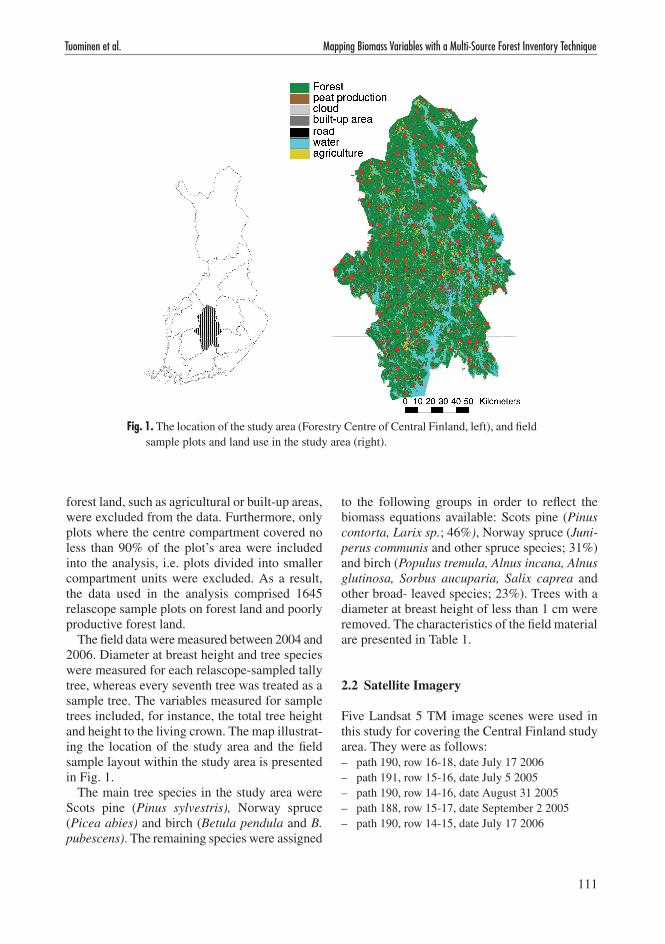
The field data were measured between 2004 and 2006. Diameter at breast height and tree species were measured for each relascope-sampled tally tree, whereas every seventh tree was treated as a sample tree. The variables measured for sample trees included, for instance, the total tree height and height to the living crown. The map illustrat-ing the location of the study area and the field sample layout within the study area is presented in Fig. 1.

The main tree species in the study area were Scots pine (Pinus sylvestris), Norway spruce (Picea abies) and birch (Betula pendula and B. pubescens). The remaining species were assigned

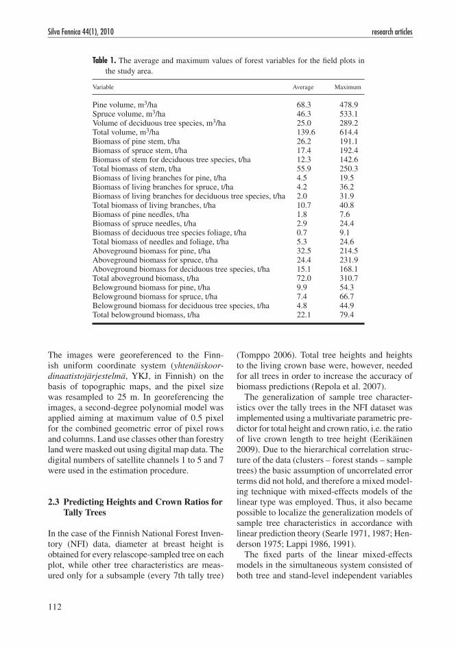
to the following groups in order to reflect the biomass equations available: Scots pine (Pinus contorta, Larix sp.; 46%), Norway spruce (Juni-perus communis and other spruce species; 31%) and birch (Populus tremula, Alnus incana, Alnus glutinosa, Sorbus aucuparia, Salix caprea and other broadleaved species; 23%). Trees with a diameter at breast height of less than 1 cm were removed. The characteristics of the field material are presented in Table 1.

2.2 Satellite Imagery

Five Landsat 5 TM image scenes were used in this study for covering the Central Finland study area. They were as follows:– path 190, row 16-18, date July 17 2006 – path 191, row 15-16, date July 5 2005 – path 190, row 14-16, date August 31 2005 – path 188, row 15-17, date September 2 2005 – path 190, row 14-15, date July 17 2006

Fig. 1. The location of the study area (Forestry Centre of Central Finland, left), and field sample plots and land use in the study area (right).

112


The images were georeferenced to the Finn-ish uniform coordinate system (yhtenäiskoor-dinaatistojärjestelmä, YKJ, in Finnish) on the basis of topographic maps, and the pixel size was re sampled to 25 m. In georeferencing the images, a second-degree polynomial model was applied aiming at maximum value of 0.5 pixel for the combined geometric error of pixel rows and columns. Land use classes other than forestry land were masked out using digital map data. The digital numbers of satellite channels 1 to 5 and 7 were used in the estimation procedure.

2.3 Predicting Heights and Crown Ratios for Tally Trees

In the case of the Finnish National Forest Inven-tory (NFI) data, diameter at breast height is obtained for every relascope-sampled tree on each plot, while other tree characteristics are meas-ured only for a subsample (every 7th tally tree)

(Tomppo 2006). Total tree heights and heights to the living crown base were, however, needed for all trees in order to increase the accuracy of biomass predictions (Repola et al. 2007).

The generalization of sample tree character-istics over the tally trees in the NFI dataset was implemented using a multivariate parametric pre-dictor for total height and crown ratio, i.e. the ratio of live crown length to tree height (Eerikäinen 2009). Due to the hierarchical correlation struc-ture of the data (clusters – forest stands – sample trees) the basic assumption of uncorrelated error terms did not hold, and therefore a mixed model-ing technique with mixed-effects models of the linear type was employed. Thus, it also became possible to localize the generalization models of sample tree characteristics in accordance with linear prediction theory (Searle 1971, 1987; Hen-derson 1975; Lappi 1986, 1991).

The fixed parts of the linear mixed-effects models in the simultaneous system consisted of both tree and stand-level independent variables

Table 1. The average and maximum values of forest variables for the field plots in the study area.

Variable Average Maximum

Pine volume, m3/ha 68.3 478.9Spruce volume, m3/ha 46.3 533.1Volume of deciduous tree species, m3/ha 25.0 289.2Total volume, m3/ha 139.6 614.4Biomass of pine stem, t/ha 26.2 191.1Biomass of spruce stem, t/ha 17.4 192.4Biomass of stem for deciduous tree species, t/ha 12.3 142.6Total biomass of stem, t/ha 55.9 250.3Biomass of living branches for pine, t/ha 4.5 19.5Biomass of living branches for spruce, t/ha 4.2 36.2Biomass of living branches for deciduous tree species, t/ha 2.0 31.9Total biomass of living branches, t/ha 10.7 40.8Biomass of pine needles, t/ha 1.8 7.6Biomass of spruce needles, t/ha 2.9 24.4Biomass of deciduous tree species foliage, t/ha 0.7 9.1Total biomass of needles and foliage, t/ha 5.3 24.6Aboveground biomass for pine, t/ha 32.5 214.5Aboveground biomass for spruce, t/ha 24.4 231.9Aboveground biomass for deciduous tree species, t/ha 15.1 168.1Total aboveground biomass, t/ha 72.0 310.7Belowground biomass for pine, t/ha 9.9 54.3Belowground biomass for spruce, t/ha 7.4 66.7Belowground biomass for deciduous tree species, t/ha 4.8 44.9Total belowground biomass, t/ha 22.1 79.4

113


such as diameter at breast height, indicators for tree species-specific effects, measurable stand characteristics and site quality indicators. The random parts of the models included parameters for cluster and stand effects along with compo-nents for tree species-specific effects. The Best Linear Unbiased Predictor (BLUP) -based local-ization of these models is applicable if either of the two sample tree characteristics is available for at least one sample tree with known (measured) independent variables (see Lappi 1991).

2.4 The Biomass Equations

In order to obtain biomass estimates for the rela-scope sampled trees of the NFI data we used equations by Repola et al. (2007); models based on crown components including diameter at breast height, height and living crown length were applied as independent variables to determine foliage and branch biomasses. Stem biomasses, by contrast, were predicted using the stem wood density models by Repola et al. (2007), con-taining diameter at breast height, tree age, tem-perature sum as independent variables, and stem volume functions by Laasasenaho (1982) for pine, spruce and birch based on height and diameter at breast height. The total aboveground biomass was obtained by combining the model-derived biomass estimates for foliage, branches and stem. The belowground biomass for spruce and birch was computed by combining the biomasses of stump and roots thicker than 1 cm. However, for estimating the belowground biomass of Scots pine, the functions by Petersson and Ståhl (2006) were used. Finally, individual biomasses of trees were summed up at the sample plot-level. For this purpose inclusion probability of tally- and sample trees was estimated on the basis of the applied relascope factor, which is 2 for the NFI set of data from Central Finland, and the distance of the tree from the plot centre.

In this study, the volume and biomass variables (applied model in parentheses) calculated at the plot-level were as follows:1) stem volumes (Laasasenaho 1982) for the groups

of Scots Pine, Norway Spruce and Birch, respec-tively, and for all trees;

2) biomass of stem (Laasasenaho 1982 & Repola et

al. 2007) for the groups of Scots Pine, Norway Spruce and Birch group, respectively, and for all trees;

3) biomass of living branches (Repola et al. 2007) for the groups of Scots Pine, Norway Spruce and Birch, respectively, and for all trees;

4) biomass of needles (Repola et al. 2007) for the groups of Scots Pine, Norway Spruce and Birch, respectively, and for all trees;

5) total aboveground biomass (Repola et al. 2007) for the groups of Scots Pine, Norway Spruce and Birch, respectively, and for all trees; and

6) total belowground biomass for Scots Pine group (Petersson and Ståhl 2006), Norway Spruce group (Repola et al. 2007) and Birch group (Repola et al. 2007), and for all trees.

2.5 k-Nearest Neighbour Estimation Method

The k nearest neighbour (k-nn) method (e.g. Kilkki and Päivinen 1987, Muinonen and Tokola 1990, Tomppo 1990) was applied for producing estimates of biomass variables in the form of thematic maps covering the area of Central Fin-land. The k-nn method is based on the assumption that NFI sample plots having similar biomass characteristics also have similar satellite image spectral features, i.e. are located near each other in the n-dimensional image feature space, where n represents the number of satellite image channels. The k nearest neighbours were determined by the Euclidean distances between the observations in the satellite image feature space. Since the satel-lite reflectance of a stand depends on the season and the atmospheric and illumination conditions and is, therefore, image scene-specific, the k-nn selection was limited to the sample plots located in the same satellite image as the target pixel. The generated biomass map was a mosaic of the k-nn estimations of individual satellite image scenes.

The satellite image channels were weighted on the basis of cross-validating the volume estimates of the tree species groups (pine, spruce, birch and other broadleaved), and the same weights were applied to the biomass variables. The parameters were optimized for minimizing the RMSE values and biases of stem volumes by different tree spe-cies. In optimizing the estimation parameters, Norway spruce and Scots pine were weighted

114


more than deciduous tree species because of their better representativeness in the study area. Ini-tially, all the field plots covered by the satellite images were utilized when computing the param-eters for the k-nn estimation procedure, such as the value of k or the weights of the satellite image channels.

The estimates of biomass variables were calcu-lated as weighted averages of the measured bio-mass variables of the k nearest neighbors (i.e. NFI plots). The k nearest neighbors were weighted by their inverse squared Euclidean distances in the feature space (Eq. 1). This method reduces the bias of the estimates (e.g. Altman 1992). The value of k varied depending on the number of NFI plots covered by a satellite: k=3 was applied with satellite images covering the smallest total number of NFI plots, whereas k=5 was applied to the remaining satellite images.

ˆ ( )yd

ydi

ii

k

ii

k

=

= =∑ ∑1 1

12

12

1

wherey = estimate for variable y yi = measured value of variable y in the ith nearest

neighbor plotdi = Euclidean distance to the ith nearest neighbor

plotk = number of nearest neighbors

Several studies have shown that when a large number of field plots are available for k-nn estima-tion, increasing the number of nearest neighbours (value of k) generally improves the accuracy of the (plot-level) estimates (e.g. Tokola et al. 1996, Nilsson 1997, Franco-Lopez et al. 2001). On the other hand, the value of k is a trade-off between the accuracy of the estimates and the variation in the original field material that is retained in the estimates. The greater the value of k, the more averaging occurs in the estimates. Thus, for example Franco-Lopez et al. (2001) have sug-gested k = 1 for the purpose of map production in order to retain the full variation of the field data in the estimates.

2.6 Cross-validating the k-nn Estimates

The biomass estimates were tested using a leave-one-out cross-validation technique, in which each sample plot in turn was left out from the set of reference plots and estimated with the aid of the remaining plots. The estimates of the field plots were compared with the corresponding values of the plots that were modelled on the basis of field measurements, thus producing a measure of their accuracy as root mean square errors, RMSE (Eq. 2), as well as their biases (Eq. 3).

RMSE =−

=∑ ( ˆ )

( )

y y

n

i ii

n2

1 2

Bias =−

=∑ ( ˆ )

( )

y y

n

i ii

n

1 3

3 Results

The cross-validation results for the biomass vari-able estimates indicate that the methodology for producing satellite image-based biomass maps is well suited for the task. The estimation accuracy of biomass variables was generally similar or even better than what typically is achieved with tradi-tional growing stock related stand variables.

The results are presented separately for peat-lands and mineral soils, because the peatland mask was applied in the classification and, there-fore, the estimation of peatlands was carried out utilizing different set of field plots than with mineral soils. The cross-validation results are presented for satellite images 188/15-17 and 190/14-16 acquired in September 2, 2005 and August 31, 2005, respectively. These two images covered almost all of the sample plots in the study area, 1555 sample plots out of the total of 1645, and part of those were covered by both images. The remaining images were used for covering the cloud areas and gaps at the edges of the study area. The image 188/15-17 covered 968 field plots on mineral soil sites and 198 field plots on peat-land sites. Image 190/14-16 had 715 field plots on

115


Table 2a. The estimation results for patched images 188/15-17. Units for the volumes and biomasses are m3/ha and tons/ha, respectively.

Variable Mineral soil Peatland

Average of estimates

RMSE % Bias % Average of estimates

RMSE % Bias %

Pine stem volume 65.4 110.3 1.3 65.7 98.4 0.1Spruce stem volume 59.6 142.0 0.2 25.7 201.9 –7.3Stem volume of deciduous tree species 25.8 172.4 –5.7 22.5 168.3 –0.6Total stem volume 150.8 67.8 –0.3 113.9 73.1 –1.7

Biomass of pine stem 25.0 111.6 1.3 25.7 98.6 0.3Biomass of spruce stem 22.3 139.9 0.6 10.0 197.0 –6.9Biomass of stem of deciduous tree species 12.7 174.1 –5.6 11.1 169.8 –0.5Total biomass of stem 60.0 69.0 –0.4 46.8 74.6 –1.4

Biomass of living branches for pine 4.2 99.4 1.9 4.4 86.8 0.0Biomass of living branches for spruce 5.2 126.5 –0.6 2.6 175.5 –7.1Biomass of living branches for deciduous tree

species2.1 164.0 –5.6 1.8 162.5 –0.6

Total biomass of living branches 11.6 58.8 –0.6 8.8 64.7 –2.2

Biomass of pine needles 1.6 98.6 2.9 1.8 85.5 1.1Biomass of spruce needles 3.6 119.6 –0.2 2.0 162.0 –6.7Biomass of deciduous tree species foliage 0.7 153.6 –6.0 0.6 147.0 –0.7Total biomass of needles and foliage 5.9 63.9 0.0 4.4 70.6 –2.7

Aboveground biomass of pine 30.8 107.8 1.5 31.9 95.4 0.3Aboveground biomass of spruce 31.1 133.7 0.3 14.6 186.2 –6.9Aboveground biomass of deciduous tree species 15.5 169.3 –5.6 13.6 166.4 –0.5Total aboveground biomass 77.4 65.1 –0.4 60.0 71.0 –1.6

Belowground biomass of pine 9.3 105.0 1.5 10.0 92.8 0.3Belowground biomass of spruce 9.3 130.3 0.0 4.6 178.2 –6.5Belowground biomass of deciduous tree species 5.0 150.0 –5.2 4.6 150.2 0.9Total belowground biomass 23.6 59.7 –0.5 19.2 65.2 –1.2

mineral soil sites and 223 field plots on peatland sites. For these satellite images the number of k used in the estimation was 5

The cross validation results of stem volume, aboveground and belowground biomass compo-nents were obtained for all tree species and by species, respectively. The relative RMSE values obtained for total volumes and biomasses were of the same magnitude. However, lower relative RMSE values were obtained for the branch and foliage biomasses compared to the stem vol-umes.

The results demonstrate very clearly that it is possible to estimate biomasses as precisely as stem volumes by satellite image based estima-tion. The RMSE values for different tree species groups were very high; in many cases the relative RMSE was over 100%. The estimation results

are presented for two main satellite images of the research area in Tables 2a and 2b.

Thematic maps for the estimated aboveground and belowground forest biomasses (tons/ha) are illustrated in Figs. 2a and 2b, respectively.

4 Discussion

When validation results of this study were com-pared to the results reported in other studies with similar data sources, the absolute and relative RMSE values obtained for the volume estimates by tree species were of the same magnitude (e.g. Katila and Tomppo 2001). Moreover, the relative RMSEs for stem volume and biomass were also of the same magnitude in this study. However, the

116


relative RMSEs obtained for the branch and foli-age biomasses were lower than that of volume.

In the case of boreal forests, the digital num-bers of the satellite image channel values are mainly based on the reflectance from: 1) the sun-illuminated parts of the tree crowns, 2) the shadowed sections of tree crowns, and 3) the ground (i.e. gaps in the crown canopy cover). The reflectance of a forest stand is highly dependent on its structural properties, such as the size, shape, volume and density of the tree crowns, size and angle of the leaves or needles, and the canopy closure (e.g. Asner 1998, Rautiainen. et al. 2004, Lang et al. 2007). Furthermore, the reflectance is also affected by the illumination conditions and the sun zenith angle; for example, in boreal areas where the solar zenith angles are typically low, the forest undergrowth is often shadowed by larger

trees (e.g. Chen and Leblanc 1997). Thus, stands with similar amounts of biomass or growing stock volumes often have different reflectance charac-teristics because of the aforementioned factors.

A high correlation between the measured canopy size, the stand density characteristics and the spectral characteristics of the satellite images could explain why the biomass variables, espe-cially the biomass in foliage and needles, seem to be estimated more accurately than stem volumes. On the other hand, there is no direct interdepend-ence between the stem volume variables and the canopy size characteristics, and thereby neither between the stem volume variables and the satel-lite image pixel values. Thus, the better estimation results obtained for the aboveground biomass variables were a logical outcome.

The belowground biomass variables, on the

Table 2b. The estimation results for patched images 190/14-16. Volume units are m3/ha and biomass units tons/ha.

Variable Mineral soil Peatland

Average of estimates

RMSE % Bias % Average of estimates

RMSE % Bias %

Pine stem volume 77.1 95.2 1.1 67.6 86.2 2.2Spruce stem volume 42.2 172.1 –4.4 17.1 228.8 –4.7Stem volume of deciduous tree species 23.0 181.4 –3.2 16.2 185.9 –9.5Total stem volume 142.3 67.9 –1.2 100.9 71.3 –0.9

Biomass of pine stem 29.4 96.7 1.0 26.5 86.6 2.0Biomass of spruce stem 16.0 170.1 –4.2 6.7 226.7 –4.8Biomass of stem of deciduous tree species 11.3 182.8 –3.1 8.1 187.4 –9.5Total biomass of stem 56.7 69.7 –1.2 41.2 73.2 –1.3

Biomass of living branches for pine 5.1 82.5 1.5 4.7 72.3 2.4Biomass of living branches for spruce 3.9 152.3 –3.2 1.8 197.8 –6.9Biomass of living branches of deciduous tree

species1.8 176.5 –3.9 1.3 186.3 –10.3

Total biomass of living branches 10.9 60.3 –1.1 7.8 61.6 –1.8

Biomass of pine needles 2.0 80.8 2.3 2.0 70.5 1.9Biomass of spruce needles 2.7 141.8 –3.1 1.4 185.3 –8.1Biomass of deciduous tree species foliage 0.6 160.8 –3.1 0.5 167.5 –9.7Total biomass of needles and foliage 5.4 64.8 –1.1 3.8 69.5 –3.2

Aboveground biomass of pine 36.6 92.3 1.2 33.2 82.6 2.1Aboveground biomass of spruce 22.6 161.7 –3.9 9.8 213.5 –5.6Aboveground biomass of deciduous tree species 13.8 177.9 –3.2 9.8 184.8 –9.6Total aboveground biomass 73.0 66.0 –1.2 52.8 69.6 –1.5

Belowground biomass of pine 11.1 88.7 1.2 10.5 80.1 2.4Belowground biomass of spruce 6.9 157.3 –3.5 3.2 202.6 –5.3Belowground biomass of deciduous tree species 4.5 160.5 –3.9 3.3 172.5 –8.3Total belowground biomass 22.4 59.6 –1.2 17.0 65.4 –1.1

117


contrary, have very little direct influence on the reflectance of a certain forest stand in a satel-lite image. Thus the successful estimation of belowground biomass mainly depends on the performance of the biomass models and the cor-relation between the biomass variables and the measured tree size characteristics. Furthermore, in the satellite image interpretation phase, the estimation success depends on the correlation between the biomass variables and the crown canopy characteristics.

The thematic maps rely on the NFI measure-ments and also on the empirical biomass models. The unexplained variation of the biomass models (Repola et al. 2007) is higher compared to that of the volume models (Laasasenaho 1982). This, in turn, leads to the fact that there is more averaging in the biomass estimates than in the stem volume estimates. According to Laasasenaho (1982), the relative prediction error for Scots pine volume was 7–8%, while it was approximately 30–40% for the foliage biomass when estimated using a similar methodology (see Repola et al. 2007).

However, the biomass data of this study were available only for the field plots within the area of the Forestry Centre of Central Finland, and there-fore the results of the study cannot be deemed to be completely representative for larger geographi-cal areas.

The estimation results for the k-nn -derived biomass components on mineral soils indicate higher precision for the groups of pine and spruce (Tables 2a and 2b) when compared to those of the birch group. In the peatland set of data, however, the reliability figures for the spruce group showed highest uncertainty in the k-nn -based biomass estimates. Even if the reliability characteristics do not unambiguously reveal the superiority of esti-mates obtained for the two groups of coniferous species, it is possible that the seasonal changes in foliage biomass may have affected, especially, the reliability of biomass estimates for the birch group (Kobayashi et al. 2007, Rautiainen et al. 2009). In this case, however, the seasonal factors affecting the results should not be overestimated since the satellite images were acquired between 5th July

Fig. 2a. Aboveground biomass (tons/ha) in the study area (land use displayed, if non-forest).

Fig. 2b. Belowground biomass (tons/ha) in the study area (land use displayed, if non-forest).

118


and 2nd September, meaning that the optical imagery originated from the main growing season when the foliage of deciduous trees has attained its physiological maturity with high assimilation capacity (Rautiainen et al. 2009). Moreover, as noted in chapter 2.5, the k-nn estimation was implemented separately for each image scene. It is therefore concluded that possible errors in the biomass estimates for the birch group caused by the seasonal variation in foliage reflectance are only minor and do not violate the generality and relevance of the results.

The results of this study support the assumption that canopy dimensions are well correlated with the amount of biomass. Thus, the plot-level bio-mass estimates can be used as input data when the k-nn -based multi-source forest inventory tech-niques are applied to the estimation of biomasses. The map form biomass estimates, in turn, should reflect other stand-level attributes such as tree size distribution, competition and canopy structure.

Spatially explicit biomass maps provide solid background information for estimating both the technical and economic potential of bioenergy. The improved information about the location and quantity of forest bioenergy is valuable due to the notable variation in the earlier estimates obtained for these resources. These maps also provide valuable information when optimal loca-tions for energy plants are explored. In the case of the greenhouse gas inventory and the research on climate change, these maps can be used, for instance, for deriving estimates for gross primary production and soil carbon change.

The approach presented here was based on the Landsat images and prediction models for tree-level characteristics, such as height, crown ratio, stem volume and biomass. This methodology could also be applicable to the tropics to meet the monitoring demands related to deforesta-tion and the REDD initiative related monitoring demands.

The preparation of digital, wall-to-wall maps for the forest biomass requires remote sensing imagery, additional biomass models and geo-graphically representative ground reference data. The costs caused by inventories in the field are high, whereas other costs related to map produc-tion are relatively low. It is also important to bear in mind while judging the general applicability of

the present approach that the field inventory pro-cedures applicable to the boreal region may not be technically appropriate in other conditions. In that case the model-based estimation procedure used in this study that was used to obtain biomasses by plot needs to be carefully verified. Future studies should also search for new and more accurate methods for the tree species detection. In addition, the applicability of the present technique for the estimation of tree and biomass increment should be studied in more detail in the future.

References

Ahti, T., Hämet-Ahti, L. & Jalas, J. 1968. Vegetation zones and their sections in northwestern Europe. Annales Botanici Fennici 5(3): 169–211.

Altman, N.S. 1992. An introduction to kernel and nearest-neighbor nonparametric regression. The American Statistician 46: 175–185.

Asner, G. 1998. Biophysical and biochemical sources of variability in canopy reflectance. Remote Sens-ing of Environment 64: 234–253.

Baccini, A., Friedl, M.A., Woodcock, C.E. & War-bington, R. 2004. Forest biomass estimation over regional scales using multisource data. Geophysical Research Letters 31(10): 1–4.

Chen, J. & Leblanc, S. 1997. A four-scale bidirectional reflectance model based on canopy architecture. IEEE Transactions on Geoscience and Remote Sensing, 35(5): 1316–1337.

Eerikäinen, K. 2009. A multivariate linear mixed-effects model for the generalization of sample tree heights and crown ratios in the Finnish National Forest Inventory. Forest Science 55(6): 480–493.

Franco-Lopez, H., Ek, A.R. & Bauer M.E. 2001. Esti-mation and mapping of forest density, volume and cover type using the k-nearest neighbors method. Remote Sensing of Environment 77: 251–274.

Henderson, C.R. 1975. Best linear unbiased estimation and prediction under a selection model. Biometrics 31(2):423–447.

IPCC. 2003. Good practice guidance for land use, land-use change and forestry. IPCC National Green-house Gas Inventories Programme. 295 p.

Karjalainen, T. & Kellomäki, S. 1996. Greenhouse gas inventory for land use changes and forestry in Finland based on international guidelines. Mitiga-

119


tion and Adaptation Strategies for Global Climate 1: 51–71.

Katila, M. & Tomppo, E. 2001. Selecting estimation parameters for the Finnish multi-source national forest inventory. Remote Sensing of Environment 76: 16–32.

Kilkki, P. & Päivinen, R. 1987. Reference sample plots to combine field measurements and satellite data in forest inventory. Department of Forest Mensuration and Management, University of Helsinki, Research Notes 19: 210–215.

Kobayashi, H., Suzuki, R. & Kobayashi, S. 2007. Reflectance seasonality and its relation to the canopy leaf area index in an eastern Siberian larch forest: Multi-satellite data and radiative transfer analysis. Remote Sensing of Environment 106: 238–252.

Laasasenaho, J. 1982. Taper curve and volume func-tions for pine, spruce and birch. Communicationes Instituti Forestalis Fenniae 108. 74 p.

Lang, M., Nilson, T., Kuusk, A., Kiviste, A. and Hordo, M. 2007. The performance of foliage mass and crown radius models in forming the input of a forest reflectance model: A test on forest growth sample plots and Landsat 7 ETM+ images. Remote Sensing of Environment 110: 445–457.

Lappi, J. 1986. Mixed linear models for analyzing and predicting change in stem form variation of Scots pine. Communicationes Instituti Forestalis Fenniae 134. 69 p.

— 1991. Calibration of height and volume equations with random parameters. Forest Science 37(3): 781–801.

Lehtonen, A., Mäkipää, R., Heikkinen, J., Sievänen, R. & Liski, J. 2004. Biomass expansion factors (BEF) for Scots pine, Norway spruce and birch according to stand age for boreal forests. Forest Ecology and Management 188: 211–224.

Muinonen, E. & Tokola T. 1990. An application of remote sensing for communal forest inventory. In: Proceedings from SNS/IUFRO workshop in Umeå 26–28 Feb. 1990 (pp. 35–42). Remote Sensing Laboratory , Swedish University of Agricultural Sciences, Umeå, Report 4.

Muukkonen, P. & Heiskanen, J. 2005. Estimating bio-mass for boreal forests using ASTER satellite data combined with standwise forest inventory data. Remote Sensing of Environment 99(4): 434–447.

Nilsson, M. 1997. Estimation of forest variables using satellite image data and airborne lidar. Doctoral thesis. Acta Universitatis Agriculturae Sueciae 17.

Petersson, H. & Ståhl, G. 2006. Functions for below-ground biomass of Pinus sylvestris, Picea abies, Betula pendula and Betula pubescens in Sweden. Scandinavian Journal of Forest Research 21, Sup-plement 7: 84–93.

Rautiainen, M., Stenberg, P., Nilson, T. & Kuusk, A. 2004. The effect of crown shape on the reflectance of coniferous stands. Remote Sensing of Environ-ment 89: 41–52.

— , Nilson, T. & Lükk, T. 2009. Seasonal reflectance trends of hemiboreal birch forests. Remote Sensing of Environment 113: 805–815.

Repola, J., Ojansuu, R. & Kukkola, M. 2007. Biomass functions for Scots pine, Norway spruce and birch in Finland. Working Papers of the Finnish Forest Research Institute 53. ISBN 978-951-40-2046-9. 28 p. URL: http://www.metla.fi/julkaisut/working-papers/2007/mwp053.htm.

Searle, S.R. 1971. Linear models. John Wiley & Sons, Inc., New York. 532 p.

— 1987. Linear models for unbalanced data. John Wiley & Sons, Inc., New York. 536 p.

Tokola, T., Pitkänen, J., Partinen S. & Muinonen, E. 1996. Point accuracy of a non-parametric method in estimation of forest characteristics with different satellite materials. International Journal of Remote Sensing 17(12): 2333–2351.

Tomppo, E. 1990. Satellite image-based national forest inventory of Finland. The Photogrammetric Journal of Finland 12(1): 115–120.

— 1993. Multi-source national forest inventory of Finland. In: Nyyssönen, A., Poso, S. & Rautala, J. (eds.). Proceedings of Ilvessalo Symposium on national forest inventories, 17–21 Aug. 1992, Finland. The Finnish Forest Research Institute Research Papers 444. p. 52–60.

— 2006. The Finnish multi-source national forest inventory – small area estimation and map pro-duction. In: Kangas, A. & Maltamo, M. (eds.). Forest inventory – methodology and applications. Springer, Netherlands. p. 195–224.

Total of 31 references

mapping biomass variables with a multi-source forest ... biomass variables with a multi-source ......

Documents