Nielsen et al. Int J Health Geogr (2017) 16:43 DOI 10.1186/s12942-017-0117-5

RESEARCH

Mapping outdoor habitat and abnormally small newborns to develop an ambient health hazard indexCharlene C. Nielsen1,2, Carl G. Amrhein1, Alvaro R. Osornio‑Vargas2* and the DoMiNO Team1,2

Abstract

Background: The geography of where pregnant mothers live is important for understanding outdoor environmental habitat that may result in adverse birth outcomes. We investigated whether more babies were born small for ges‑tational age or low birth weight at term to mothers living in environments with a higher accumulation of outdoor hazards.

Methods: Live singleton births from the Alberta Perinatal Health Program, 2006–2012, were classified according to birth outcome, and used in a double kernel density estimation to determine ratios of each outcome per total births. Individual and overlay indices of spatial models of 136 air emissions and 18 land variables were correlated with the small for gestational age and low birth weight at term, for the entire province and sub‑provincially.

Results: There were 24 air substances and land sources correlated with both small for gestational age and low birth weight at term density ratios. On the provincial scale, there were 13 air substances and 2 land factors; sub‑provincial analysis found 8 additional air substances and 1 land source.

Conclusion: This study used a combination of multiple outdoor variables over a large geographic area in an objec‑tive model, which may be repeated over time or in other study areas. The air substance‑weighted index best identi‑fied where mothers having abnormally small newborns lived within areas of potential outdoor hazards. However, individual air substances and the weighted index provide complementary information.

Keywords: Small for gestational age, Low birth weight at term, Pollution, GIS, Index

© The Author(s) 2017. This article is distributed under the terms of the Creative Commons Attribution 4.0 International License (http://creativecommons.org/licenses/by/4.0/), which permits unrestricted use, distribution, and reproduction in any medium, provided you give appropriate credit to the original author(s) and the source, provide a link to the Creative Commons license, and indicate if changes were made. The Creative Commons Public Domain Dedication waiver (http://creativecommons.org/publicdomain/zero/1.0/) applies to the data made available in this article, unless otherwise stated.

BackgroundA truly ecologically-based study of health integrates habitat, population, and behavior—encompassing a more complete geography as framed by Meade’s triangle of human ecology [1, 2]. Three vertices conceptualize what is known about an important pediatric topic: maternal exposure to outdoor pollution and neonatal outcomes (Fig. 1). Here we focus on the lesser studied habitat ver-tex, specifically the outdoor environment, since less attention is traditionally given to incorporating ecological factors in understanding disease [1]. The location aspect of habitat—where pregnant women live, where industry

and services are situated, where demographic groups congregate—is important because where one lives and where one starts out in life, even during fetal develop-ment, ultimately influences lifelong health [3–6].

Toxicant exposures and environmental influences on mothers during crucial stages of pregnancy may result in newborns that are too small or born too early. Adverse birth outcomes (ABO) are important markers of infant survival, development and future health. Our research focuses on being born too small, clinically defined as Small for Gestational Age (SGA) when newborns are below the 10th percentile weight based on sex and weeks of pregnancy, or Low Birth Weight at Term (LBWT) when newborns are less than 2500 g weight at term, 37 or more weeks gestation [7].

Open Access

International Journal of Health Geographics

*Correspondence: osornio@ualberta.ca 2 Department of Pediatrics, University of Alberta, 3‑591 ECHA, 11,405 87th Avenue, Edmonton, AB T6G 1C9, CanadaFull list of author information is available at the end of the article

Page 2 of 21Nielsen et al. Int J Health Geogr (2017) 16:43

The province of Alberta, Canada, had a population of 3,645,257 at the 2011 Census [8]. That was a 10.8% increase from 2006 while the national average increase was 5.9%. For a land area of 640,082 km2, the population density was 5.7 persons/km2, where 83% of the popula-tion lived in or near urban centers. Alberta’s economic activities were focused on agriculture, natural resources, and nonrenewable energy—having a higher number of industrial facilities reporting to the National Pollutant Release Inventory (NPRI) than any other province or ter-ritory [9]. The NPRI is a valuable data source on indus-trial-based pollutants [10]. Alberta also has higher ABOs: SGA was 8.8% (Canada was 8.4%); and low birth weight for all gestational ages was 6.7% (Canada was 6.0%) [11]. Alberta rates also increased during 2000–2014: SGA from 10 to 11.5%; and low birth weight for all gestational ages from 6.1 to 6.7% [12].

ABO complications include death, physical and cogni-tive disabilities, and chronic health problems later in life, costing emotional stress and the majority of the health care expenses among all newborns [13]. Disorders related to short gestation and low birth weight are consistently ranked as the 2nd leading cause of infant death (con-genital deformation is the leading cause) [14]—and have increased in Canada since the year 2000 [11, 12].

Abnormally small newborns are the result of growth restriction, which may be due to environmental pollut-ants thought to cause inflammation in mothers, direct toxic effects on the placenta and the fetus, interruption of oxygen-hemoglobin, or DNA damage represented by the formation of DNA adducts [15, 16].

The environment includes social, built, and natural fea-tures. Individual risks are also very important to ABOs, but are neither readily available nor easily mapped. These include personal, behavioral, social, and indoor expo-sures, such as: adequate prenatal care; food type and con-taminants; rest, stress, and pre-existing health conditions; occupation and socioeconomic status; smoking and other substance use; drinking water contaminants. Our focus is on the outdoor environmental habitat because it is a common source of shared exposures susceptible to regu-lation (biology and behavior are not). These include air, water, human-constructed, and natural outdoor hazards, such as: industrial emissions; traffic pollution; agricul-tural chemical inputs of pesticides, herbicides, and ferti-lizers; electromagnetic radiation; proximity to oil and gas extraction activities; wildfire smoke.

Environmental health research has found many envi-ronmental factors to be associated with various health outcomes [17–25]. However, these are typically explored

Fig. 1 Meade’s triangle of human ecology for maternal exposures and small for gestational age (SGA) and low birth weight at term (LBWT): dashed arrow indicates hypothesized mechanisms

Page 3 of 21Nielsen et al. Int J Health Geogr (2017) 16:43

singly: one exposure or category of exposure at a time. A unified environmental measure may be constructed across multiple variables to encompass the complex nature of the overall environment.

Environmental indices have history: Inhaber had pro-posed an integrated national index for Canada in the 1970s [26]. Rather than relying on individual pollutants to reflect the state-of-the-environment, Inhaber math-ematically combined such indicators for the purpose of resource allocation, ranking of locations, enforcement of standards, trend analysis, public information, or scien-tific research [27]. Under that premise, Messer et al. [28] developed a California county-level environmental qual-ity index using principal components analysis (PCA) to calculate 5 environmental domains (air, water, land, built, and sociodemographic), which were then combined into a single index using PCA on the first components, and stratified by rural–urban continuum codes. Similarly, Messer et  al.’s CalEnviroScreen 2.0 [29, 30] superim-posed 19 individual indicators that related to pollution exposures, environmental conditions, and population characteristics, weighted and summed each set of indica-tors, and then multiplied together pollution and popu-lation (i.e. Threat ×  Vulnerability =  Risk). We have not found similar environmental health indices available for Canada, or the province of Alberta, and especially none focused primarily on maternal exposures associated with ABO.

Using a Geographical Information System (GIS), we developed a simplified and reproducible index for Alberta by estimating and aggregating pollutants from communal outdoor factors. GIS supports the inclusion of diverse data and enables modelling of hazard-exposure-dose–response processes in space [31, 32]. To capture the relevant pollutant estimates, spatially and tempo-rally appropriate GIS data files were overlaid to develop a vulnerability map of combined disparate (in theme and measurement units) environmental factors, similar to Messer et al. [28, 29]. The index will aid our examination of maternal ambient health hazards and abnormally small newborns by providing a relative ranking of locations across the province that are not limited by administrative boundaries.

Our research is part of the Data Mining and Neonatal Outcomes (DoMiNO) project that is exploring the col-location of adverse birth outcomes and environmental variables in Canada [33]. For our geographical perspec-tive on the project we hypothesized that SGA or LBWT babies are more likely to be born to mothers living in environments with a higher number of outdoor hazards (especially pollutants) than in relatively healthier habi-tats with fewer exposure hazards. Our objective was to examine how the separate and combined exposures to

the outdoor built-up, natural, and social environments of pregnant mothers coincided with patterns in adverse birth outcomes (ABO). We also expected that the large Alberta province would have regional variations in the outdoor environment and investigated this effect on the associations.

MethodsGIS parametersWe used Esri’s ArcGIS Desktop 10.5 software to perform all spatial database processing, management, distribution analyses, hazard estimations, and index calculations [34]. Proximity was extremely important in our spatial analy-sis; therefore, we customized an Alberta-focused map projection, based on the following parameters: name Azi-muthal Equidistant; central meridian − 113.5; latitude of origin 53.5; linear unit meter (1.0); and geographic coor-dinate system (GCS) datum North American 1983 (NAD 1983). We projected all GIS data to this distance-preserv-ing spatial reference.

For raster files we used a 250 m by 250 m cell size to reasonably represent both urban and rural areas in the very large study area, and to match the coarsest dataset: MODIS Terra satellite [35].

Because Alberta is landlocked, we included data features within 50  km surrounding the provincial boundary where available: by doing so, any potential pol-lutant source close to the outer edge of the province was included.

Regional attributionWe produced sub-provincial maps of the percent ratios for each ABO to facilitate comparisons more meaning-ful to health care and environmental management. We assigned administrative attributes to postal code loca-tions. This allowed grouping by health region [36] or airshed zone [37] because both are health-related admin-istrative boundaries that help identify where there may be different outdoor factors of importance.

Health regions are designated by the provincial Min-istry of Health to identify geographic areas where hos-pital boards or regional health authorities administer and deliver public health care, and are subject to change [38]. At the start of our study period, there were 9 health regions for Alberta (Table  2): Chinook Regional Health Authority (4821); Palliser Health Region (4822); Calgary Health Region (4823); David Thompson Regional Health Authority (4824); East Central Health (4825); Capital Health (4826); Aspen Regional Health Authority (4827); Peace Country Health (4828); and Northern Lights Health Region (4829).

Airshed zones are endorsed by the multi-stake-holder Clean Air Strategic Alliance (CASA) to identify

Page 4 of 21Nielsen et al. Int J Health Geogr (2017) 16:43

geographic areas where the air quality is similar in emission sources, volumes, impacts, dispersion and administrative characteristics [39]. Because Alberta has several unique topographical, meteorological, or eco-logical conditions for resolving air quality, there are 9 airsheds currently recognized (Table  2): Alberta Capi-tal Airshed Alliance (ACAA); Calgary Region Airshed Zone (CRAZ); Fort Air Partnership (FAP); Lakeland Industry and Community Association (LICA); Palliser Airshed Society (PAS); Parkland Airshed Manage-ment Zone (PAMZ); Peace Airshed Zone Association (PASZA); West Central Airshed Society (WCAS); and Wood Buffalo Environmental Association (WBEA). It is important to note that the entire province is not monitored by airshed zones, with the southwest corner, east-central, and majority of the north having no air-shed (NA).

Dependent variablesThe Alberta Perinatal Health Program (APHP) pro-vided anonymized data for the province of Alberta, from 2006 to 2012 [40]. We obtained ethics approval from the Research Ethics Board at the University of Alberta and the APHP.

We selected for live single births between 22 and 42  weeks gestation, and geocoded them to the centroid of the 6-character postal code of the mothers’ residences at the time of the birth registration. DMTI Spatial’s Plati-num Postal Code Suite [41] provided the longitude and latitude coordinates for the years 2001–2013, which we uniquely selected to guarantee static locations through the entire study period. 95% of the original data had valid coordinates for use in spatial analyses. Using the previous definitions, we classified the birth records as binary vari-ables identifying SGA or LBWT. Details are available in Serrano et al. [42].

To eliminate the confines of arbitrary administra-tive boundaries, we followed the double kernel den-sity (DKD) method [43–48] to calculate distributions of SGA and LBWT, normalized by all births. DKD involves kernel density estimation—a non-parametric method that spreads point values across a surface by calculating the magnitude-per-unit area from points (representing the counts of birth events), fitted to a smoothly tapered function that spreads the values within a specified dis-tance (25  km for this study) around each point [49]. Points within the radius that are further from the center are weighted lower than those closer, and helps indicate “hot spots”. Dividing each ABO by the kernel density of total births yielded ratios of the birth outcome that also masked locations of the residences, helping protect privacy.

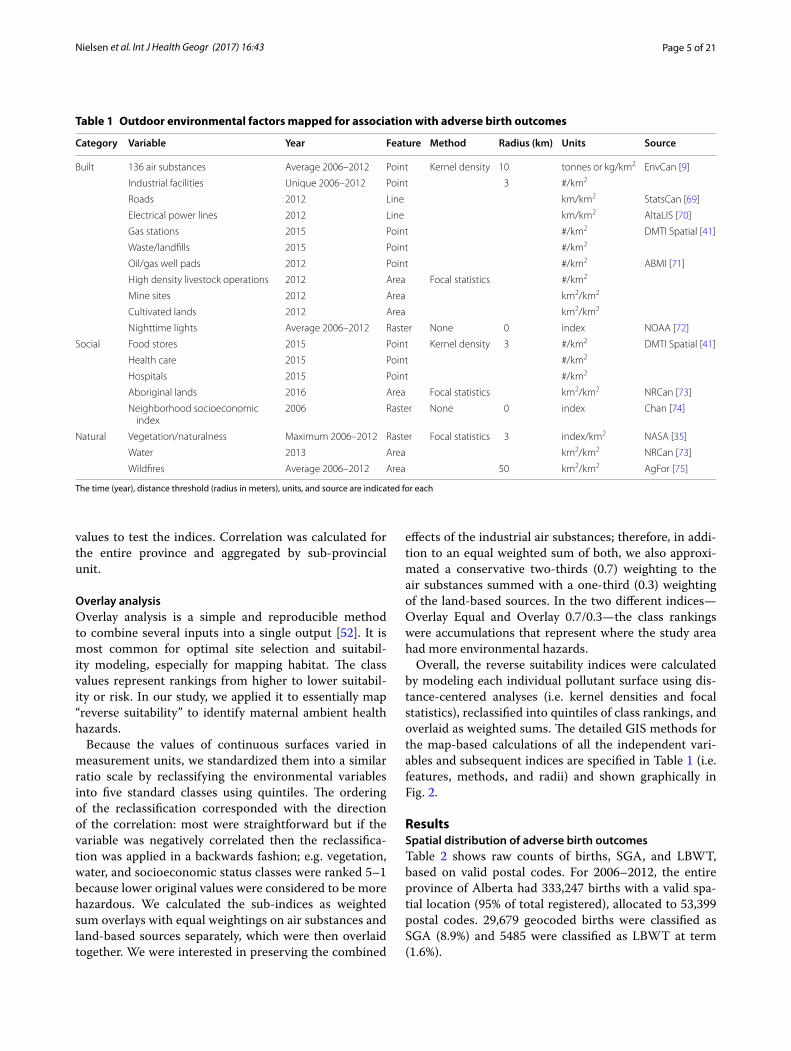
Independent variablesPersonal maternal monitoring data were not available for this retrospective study. We used landscape features as spatial proxies of exposure hazards, as done in previ-ously published research [32]. In total, we chose 18 out-door sources, identified in published studies [17–23] or added for novel exploration (10 built; 5 social; 3 natural) plus 136 industrial air substance emissions. Table 1 lists the environmental variables and indicates specific char-acteristics and processing details.

We applied kernel density to spread industrial emis-sions from the NPRI database as tonnes per area within a 10 km radius (based on distances determined from the project’s data mining algorithm [33]). We used the count of other point features—industrial facilities, gas stations, waste/landfills, oil/gas well pads, food stores, and health care/hospitals—in kernel density to calculate the num-ber per area within a 3-km radius. We also applied ker-nel density to roads and electrical power lines to calculate length per area within a 3-km radius. A main advantage of using kernel density is it accounts for distance decay (features have less influence further away). When lin-ear features are the input it also helps to approximate the number of intersections—important when analyz-ing pollution sources from roads because vehicles idle at intersections.

For areal features, we used focal statistics, also known as moving-window or neighborhood analyses, on binary surfaces of feedlots, mine sites, cultivated lands, abo-riginal lands, water/blue space, and wildfires. The mean statistic on binary values of 1, indicating presence of the feature, and 0, indicating absence, yielded proportions. For vegetation/naturalness, the mean statistic returned the mean Normalized Difference Vegetation Index (NDVI), where higher values identify more chlorophyll-producing healthy green vegetation captured by the satel-lite imagery pixels. Except for the 50-km wildfire radius, all others had a 3-km radius. We accepted the original values for the coarser resolution nighttime lights and area-based, neighborhood-level socioeconomic index.

Spearman’s rank correlationWe joined values from the DKD distributions and each independent variable surface extracted to unique postal codes where births occurred. Our data were non-nor-mally distributed due to many zero values in both the dependent and independent variables. We used Python 2.7 software [50] with the pandas 0.16 site package [51] to calculate Spearman’s rank correlations among ABO and each environmental variable. To test the association of the combined environmental factors, we calculated a second set of Spearman’s rank correlations using DKD

Page 5 of 21Nielsen et al. Int J Health Geogr (2017) 16:43

values to test the indices. Correlation was calculated for the entire province and aggregated by sub-provincial unit.

Overlay analysisOverlay analysis is a simple and reproducible method to combine several inputs into a single output [52]. It is most common for optimal site selection and suitabil-ity modeling, especially for mapping habitat. The class values represent rankings from higher to lower suitabil-ity or risk. In our study, we applied it to essentially map “reverse suitability” to identify maternal ambient health hazards.

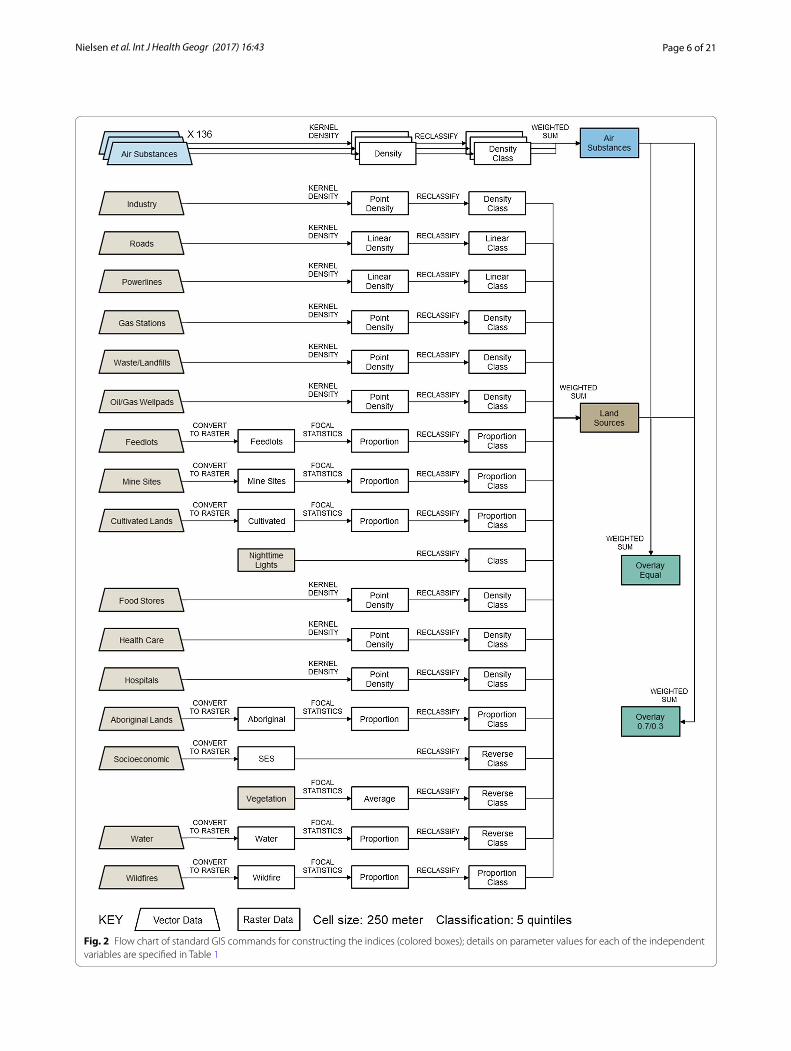
Because the values of continuous surfaces varied in measurement units, we standardized them into a similar ratio scale by reclassifying the environmental variables into five standard classes using quintiles. The ordering of the reclassification corresponded with the direction of the correlation: most were straightforward but if the variable was negatively correlated then the reclassifica-tion was applied in a backwards fashion; e.g. vegetation, water, and socioeconomic status classes were ranked 5–1 because lower original values were considered to be more hazardous. We calculated the sub-indices as weighted sum overlays with equal weightings on air substances and land-based sources separately, which were then overlaid together. We were interested in preserving the combined

effects of the industrial air substances; therefore, in addi-tion to an equal weighted sum of both, we also approxi-mated a conservative two-thirds (0.7) weighting to the air substances summed with a one-third (0.3) weighting of the land-based sources. In the two different indices—Overlay Equal and Overlay 0.7/0.3—the class rankings were accumulations that represent where the study area had more environmental hazards.

Overall, the reverse suitability indices were calculated by modeling each individual pollutant surface using dis-tance-centered analyses (i.e. kernel densities and focal statistics), reclassified into quintiles of class rankings, and overlaid as weighted sums. The detailed GIS methods for the map-based calculations of all the independent vari-ables and subsequent indices are specified in Table 1 (i.e. features, methods, and radii) and shown graphically in Fig. 2.

ResultsSpatial distribution of adverse birth outcomesTable  2 shows raw counts of births, SGA, and LBWT, based on valid postal codes. For 2006–2012, the entire province of Alberta had 333,247 births with a valid spa-tial location (95% of total registered), allocated to 53,399 postal codes. 29,679 geocoded births were classified as SGA (8.9%) and 5485 were classified as LBWT at term (1.6%).

Table 1 Outdoor environmental factors mapped for association with adverse birth outcomes

The time (year), distance threshold (radius in meters), units, and source are indicated for each

Category Variable Year Feature Method Radius (km) Units Source

Built 136 air substances Average 2006–2012 Point Kernel density 10 tonnes or kg/km2 EnvCan [9]

Industrial facilities Unique 2006–2012 Point 3 #/km2

Roads 2012 Line km/km2 StatsCan [69]

Electrical power lines 2012 Line km/km2 AltaLIS [70]

Gas stations 2015 Point #/km2 DMTI Spatial [41]

Waste/landfills 2015 Point #/km2

Oil/gas well pads 2012 Point #/km2 ABMI [71]

High density livestock operations 2012 Area Focal statistics #/km2

Mine sites 2012 Area km2/km2

Cultivated lands 2012 Area km2/km2

Nighttime lights Average 2006–2012 Raster None 0 index NOAA [72]

Social Food stores 2015 Point Kernel density 3 #/km2 DMTI Spatial [41]

Health care 2015 Point #/km2

Hospitals 2015 Point #/km2

Aboriginal lands 2016 Area Focal statistics km2/km2 NRCan [73]

Neighborhood socioeconomic index

2006 Raster None 0 index Chan [74]

Natural Vegetation/naturalness Maximum 2006–2012 Raster Focal statistics 3 index/km2 NASA [35]

Water 2013 Area km2/km2 NRCan [73]

Wildfires Average 2006–2012 Area 50 km2/km2 AgFor [75]

Page 6 of 21Nielsen et al. Int J Health Geogr (2017) 16:43

Fig. 2 Flow chart of standard GIS commands for constructing the indices (colored boxes); details on parameter values for each of the independent variables are specified in Table 1

Page 7 of 21Nielsen et al. Int J Health Geogr (2017) 16:43

Figure  3 depicts the percentages of ABO for each sub-provincial unit relative to Alberta (marked by *). For health regions, SGA ranged from 7.0 to 10.3% and LBWT ranged from 1.2 to 1.9%. Health region 4823 had

the highest number of births (n = 121,965), highest SGA (n = 12,543, 10.3%), and highest LBWT (n = 2339, 1.9%); 4825 had the lowest number of births (n =  9737), SGA (n = 698, 7.2%), and LBWT (n = 140, 1.4%); but 4827 had

Table 2 Alberta’s sub-provincial units and descriptive statistics, in descending order of birth number

Unit Map code Name Area (km2) Postal codes Geolocated births SGA LBWT

Province none Alberta 663,563 53,399 333,247 29,679 5485

Health Region 4823 Calgary Health Region 39,350 20,537 121,965 12,543 2339

4826 Capital Health 11,883 20,004 99,691 8596 1566

4824 David Thompson Regional Health Authority 61,578 3325 29,766 2394 476

4827 Aspen Regional Health Authority 137,639 1440 18,004 1252 222

4821 Chinook Regional Health Authority 26,062 2406 16,639 1342 233

4828 Peace Country Health 123,870 1580 16,428 1188 215

4829 Northern Lights Health Region 189,696 1073 11,097 808 147

4822 Palliser Health Region 39,772 1723 9920 858 147

4825 East Central Health 33,812 1311 9737 698 140

Airshed Zone CRAZ Calgary Regional Airshed Zone 32,372 20,530 120,392 12,409 2310

ACAA Alberta Capital Airshed Alliance 4933 19,474 95,085 8284 1503

NA No Airshed Zone 362,439 4867 47,527 3509 647

PAMZ Parkland Airshed Management Zone 40,936 2774 24,896 1978 387

PASZA Peace Airshed Zone Association 45,892 1409 12,475 927 175

PAS Palliser Airshed Society 39,900 1723 9920 858 147

WBEA Wood Buffalo Environmental Association 69,214 1061 7540 627 115

WCAS West Central Airshed Society 47,142 612 7386 559 107

LICA Lakeland Industrial Community Association 16,215 455 4479 293 43

FAP Fort Air Partnership 4519 494 3547 235 51

Fig. 3 Percentages of births having small for gestational age (SGA) or low birth weight at term (LBWT) in sub‑provincial units (* indicates value for the whole province)

Page 8 of 21Nielsen et al. Int J Health Geogr (2017) 16:43

the lowest SGA (n =  1252, 7.0%) and LBWT (n =  222, 1.2%). For airshed zones, SGA ranged from 6.5 to 10.3% and LBWT ranged from 1.0 to 1.9%. Airshed zone CRAZ had the highest number of births (n  =  120,392), SGA (n =  12,409, 10.3%), and LBWT (n =  2310, 1.9%); FAP had the lowest number of births (n =  3.547) and LICA had the lowest SGA (n =  293, 6.5%) and lowest LBWT (n = 43, 1.0%).

The distributions of births per area in Fig. 4 show higher concentrations of more than 3 births per km2 in the sub-provincial units containing the major cities of Edmonton and Calgary, with medium densities in the adjacent units and in the airshed zones containing Grande Prairie (west-central) and Cold Lake (east-central).

The patterns differ by sub-provincial unit for ABOs mapped as numbers per births (Fig.  5). SGA is highest in the units containing Edmonton and along the west–east Banff–Calgary-Brooks corridor. Health regions have medium SGA adjacent to the high SGA. Airsheds also show medium SGA in the west and north-east. LBWT is highest in the north–south Edmonton-Red Deer-Calgary corridor. Medium LBWT is adjacent to the higher units, except for the northern health regions containing Grande

Prairie-Peace River and Fort McMurray-Fox Lake. The lower LBWT in the central health region 4827 separates the province; LBWT in the airshed containing Cold Lake is the lowest in the province.

Figure 6 maps the results of the DKD method for each ABO. Both ABOs cover the same areas of the province and the darker colors indicate higher values for SGA (purple) and LBWT (green). The result of DKD is a con-tinuous value, but the maps classified with tertiles visu-ally enhance the slightly different distributions for SGA and LBWT: urban (Edmonton and Calgary) areas shared highest values for both ABO; central areas had more LBWT; and southeast areas had more SGA.

Hazard mappingThe Spearman’s rank correlation values were sorted in descending order for each of the independent vari-ables (Table  3). Provincially, variables having correla-tions greater than 0.40 (low value accepted since data were not adjusted for epidemiological factors because they were not available for mapping) with SGA were: i-Butyl alcohol (rho  =  0.56); Asbestos; Nighttime Light; Toluenediisocyanate; Toluene-2,4-diisocyanate;

Fig. 4 Births per area ratios in sub‑provincial units

Page 9 of 21Nielsen et al. Int J Health Geogr (2017) 16:43

Fig. 5 Adverse birth outcome (ABO) ratios in sub‑provincial units

Page 10 of 21Nielsen et al. Int J Health Geogr (2017) 16:43

Toluene-2,6-diisocyanate; Chromium Aluminum; Hydrogen sulphide; Road; 2-Ethoxyethanol; *Nickel; Qui-noline; Aniline; Cyclohexane; Acetaldehyde; and *Phos-phorus (rho =  0.42). Variables with correlations greater than 0.40 with LBWT were: i-Butyl alcohol (rho = 0.54); Asbestos; Toluenediisocyanate; Toluene-2,4-diisocy-anate; Toluene-2,6-diisocyanate; Aluminum; Chromium; Nighttime Light; Hydrogen sulphide; 2-Ethoxyethanol; Quinoline; Aniline; Road; Cyclohexane; Acetaldehyde; *Isopropyl alcohol; and *Ethylene oxide (rho  =  0.41). Both ABOs were strongly associated with 15 air sub-stances (the asterisk * marks those that differed: Nickel and Phosphorous for SGA; Ethylene oxide and Isopropyl alcohol for LBWT) and 2 land sources (both Nighttime Light and Road). Both ABOs had negative correlations (< −  0.40) with Vegetation (SGA rho = −  0.56; LBWT rho  =  −  0.48), Oil/Gas Wellpad (SGA rho  =  −  0.53; LBWT rho  =  −  0.49), and Cultivated Land (SGA rho = − 0.47; LBWT rho = − 0.41).

The dilution effect of spreading the hazards across the large study area highlighted regional importance. Using the criteria of four or more health regions having a rho greater than 0.40 indicated the importance of Nitrogen

oxides, Sulphur dioxide, Particulate Matter less than or equal to 2.5 μ (PM2.5), and Acetaldehyde with SGA. The same criteria identified Xylene, Mine Site, Manganese, and Lead for LBWT. Four or more airshed zones having a rho greater than 0.40 highlighted Sulphur dioxide and Acetaldehyde with SGA, and Xylene, Particulate Matter less than or equal to 10 microns (PM10), and PM2.5 for LBWT.

The number of unique environmental variables having rho values greater than 0.40 province-wide or within four or more sub-provincial units totaled 30 (24 air substances and 6 land-based).

Spatial distribution of the indicesFigure 7 maps the results from the weighted overlay sum of the five class rankings for 136 emitted air substances, 18 land sources, the overlay equal weighting of both, and the Overlay 0.7/0.3 weighting of air substances and land. The distribution of the higher rankings spatially coincides with Alberta’s populated places, except for higher values along the foothills, the Fort McMurray oil sands area in the north, and some scattered areas in the northeast.

Fig. 6 Double kernel density (DKD) distributions of small for gestational age (SGA) and low birth weight at term (LBWT) are ratios of the adverse birth outcome (ABO) per area divided by total births per area, each within a 25 km radius; DKD is dimensionless

Page 11 of 21Nielsen et al. Int J Health Geogr (2017) 16:43

Table 3 Spearman’s rank correlations of small for gestational age (SGA) and low birth weight at term (LBWT) with air sub-stances and land sources (*), in descending correlation rho values

Variable Province rho Health Region count (rho range) Airshed Zone count (rho range)

SGA LBWT SGA LBWT SGA LBWT

i‑Butyl alcohol 0.56 0.54 1 (0.02 to 0.81) 3 (0.42 to 0.80) 1 (0.32 to 0.81) 2 (0.45 to 0.80)

Asbestos (friable form) 0.54 0.52 1 (0.73 to 0.73) 1 (0.67 to 0.67) 1 (0.73 to 0.73) 1 (0.67 to 0.67)

*Nighttime Light 0.51 0.47 2 (− 0.17 to 0.48) 1 (− 0.50 to 0.42) 2 (− 0.40 to 0.51) 3 (− 0.50 to 0.52)

Toluenediisocyanate (mixed isomers) 0.49 0.51 0 (0.26 to 0.26) 1 (0.42 to 0.42) 0 (0.26 to 0.26) 1 (0.42 to 0.42)

Toluene‑2,4‑diisocyanate 0.49 0.50 0 (0.26 to 0.26) 1 (0.41 to 0.41) 0 (0.26 to 0.26) 1 (0.41 to 0.41)

Toluene‑2,6‑diisocyanate 0.49 0.50 0 (0.26 to 0.26) 1 (0.41 to 0.41) 0 (0.26 to 0.26) 1 (0.41 to 0.41)

Chromium (and its compounds) 0.48 0.47 2 (− 0.07 to 0.68) 2 (− 0.07 to 0.77) 2 (− 0.23 to 0.68) 2 (− 0.26 to 0.77)

Aluminum (fume or dust) 0.48 0.49 1 (0.20 to 0.67) 1 (0.25 to 0.76) 1 (− 0.18 to 0.67) 1 (− 0.20 to 0.76)

Hydrogen sulphide 0.47 0.47 4 (− 0.09 to 0.59) 3 (− 0.06 to 0.67) 3 (− 0.34 to 0.59) 3 (− 0.35 to 0.67)

*Road 0.46 0.42 2 (− 0.11 to 0.47) 0 (− 0.37 to 0.38) 3 (− 0.01 to 0.60) 2 (− 0.37 to 0.51)

2‑Ethoxyethanol 0.44 0.46 0 (0.25 to 0.25) 1 (0.41 to 0.41) 0 (0.25 to 0.25) 1 (0.41 to 0.41)

Nickel (and its compounds) 0.44 0.39 2 (− 0.20 to 0.66) 3 (− 0.88 to 0.75) 2 (− 0.24 to 0.66) 2 (− 0.88 to 0.75)

Quinoline (and its salts) 0.43 0.46 0 (0.25 to 0.25) 1 (0.40 to 0.40) 0 (0.25 to 0.25) 1 (0.40 to 0.40)

Aniline (and its salts) 0.43 0.45 0 (0.25 to 0.25) 1 (0.40 to 0.40) 0 (0.25 to 0.25) 1 (0.40 to 0.40)

Cyclohexane 0.42 0.42 3 (− 0.07 to 0.81) 3 (− 0.07 to 0.81) 3 (− 0.27 to 0.81) 3 (− 0.30 to 0.81)

Acetaldehyde 0.42 0.42 4 (− 0.41 to 0.60) 3 (− 0.07 to 0.59) 4 (− 0.34 to 0.60) 3 (− 0.34 to 0.59)

Phosphorus (total) 0.42 0.38 1 (− 0.20 to 0.49) 1 (− 0.88 to 0.44) 1 (− 0.49 to 0.52) 1 (− 0.88 to 0.46)

Isopropyl alcohol 0.40 0.41 2 (− 0.40 to 0.52) 3 (− 0.47 to 0.53) 2 (− 0.60 to 0.77) 2 (− 0.67 to 0.52)

PAHs, Total unspeciated 0.40 0.40 0 (0.30 to 0.32) 1 (0.33 to 0.43) 0 (0.26 to 0.32) 1 (0.29 to 0.43)

Ethylene oxide 0.36 0.41 0 (− 0.43 to 0.25) 1 (− 0.20 to 0.41) 0 (− 0.30 to 0.25) 1 (− 0.32 to 0.41)

Ammonia (total) 0.36 0.34 1 (− 0.41 to 0.63) 1 (− 0.75 to 0.73) 1 (− 0.50 to 0.53) 1 (− 0.75 to 0.66)

Phosphorus (yellow or white) 0.35 0.37 0 (− 0.14 to 0.05) 0 (− 0.14 to 0.23) 0 (− 0.15 to 0.05) 0 (− 0.14 to 0.23)

Methylenebis(phenylisocyanate) 0.34 0.38 0 (− 0.43 to 0.23) 0 (− 0.49 to 0.38) 0 (0.13 to 0.23) 1 (0.38 to 0.72)

PM10—Particulate Matter <= 10 Microns 0.33 0.30 3 (− 0.33 to 0.89) 3 (− 0.83 to 0.62) 3 (− 0.75 to 0.93) 4 (− 0.83 to 0.68)

n‑Butyl alcohol 0.31 0.32 1 (− 0.71 to 0.79) 1 (− 0.75 to 0.81) 1 (0.19 to 0.79) 1 (0.36 to 0.81)

Dichloromethane 0.31 0.31 1 (0.27 to 0.72) 2 (0.42 to 0.74) 1 (− 0.22 to 0.71) 2 (− 0.25 to 0.73)

Ethylene 0.30 0.33 3 (0.02 to 0.80) 3 (0.02 to 0.79) 3 (− 0.32 to 0.80) 3 (− 0.33 to 0.79)

Styrene 0.30 0.31 1 (0.00 to 0.81) 1 (− 0.01 to 0.82) 1 (− 0.32 to 0.83) 1 (− 0.32 to 0.85)

Lead (and its compounds) 0.30 0.30 3 (− 0.07 to 0.68) 4 (− 0.26 to 0.76) 3 (− 0.23 to 0.87) 3 (− 0.65 to 0.76)

*Food Store 0.28 0.28 1 (− 0.18 to 0.58) 1 (− 0.23 to 0.57) 2 (− 0.18 to 0.58) 1 (− 0.17 to 0.57)

Cumene 0.27 0.27 1 (0.29 to 0.58) 2 (0.44 to 0.61) 1 (− 0.14 to 0.57) 2 (− 0.09 to 0.60)

Methyl isobutyl ketone 0.25 0.26 1 (0.07 to 0.69) 1 (0.25 to 0.73) 1 (0.07 to 0.67) 1 (0.08 to 0.71)

Xylene (mixed isomers) 0.24 0.26 1 (− 0.71 to 0.54) 5 (− 0.74 to 0.59) 2 (− 0.65 to 0.74) 5 (− 0.47 to 0.87)

Sulphur dioxide 0.24 0.20 5 (− 0.27 to 0.88) 3 (− 0.87 to 0.74) 4 (− 0.35 to 0.91) 2 (− 0.87 to 0.68)

Manganese (and its compounds) 0.24 0.21 3 (− 0.03 to 0.68) 4 (− 0.34 to 0.72) 3 (− 0.50 to 0.65) 3 (− 0.71 to 0.70)

Fluorene—PAH 0.23 0.13 2 (− 0.32 to 0.50) 2 (− 0.89 to 0.55) 2 (− 0.49 to 0.52) 2 (− 0.89 to 0.53)

2‑Butoxyethanol 0.22 0.23 1 (− 0.69 to 0.66) 1 (− 0.70 to 0.66) 1 (0.11 to 0.64) 1 (0.11 to 0.64)

*Gas Station 0.20 0.20 1 (− 0.23 to 0.58) 0 (− 0.25 to 0.30) 2 (− 0.41 to 0.56) 1 (− 0.42 to 0.58)

Naphthalene 0.20 0.14 1 (− 0.21 to 0.59) 2 (− 0.89 to 0.63) 1 (− 0.40 to 0.61) 2 (− 0.89 to 0.65)

Propylene 0.18 0.19 1 (− 0.11 to 0.68) 1 (− 0.01 to 0.71) 1 (− 0.30 to 0.70) 1 (− 0.31 to 0.73)

*Health Care 0.17 0.17 2 (− 0.21 to 0.51) 0 (− 0.36 to 0.24) 2 (− 0.22 to 0.53) 0 (− 0.49 to 0.28)

Volatile Organic Compounds (VOCs) 0.17 0.15 3 (− 0.45 to 0.88) 2 (− 0.74 to 0.67) 2 (− 0.45 to 0.92) 1 (− 0.74 to 0.69)

Toluene 0.17 0.19 1 (− 0.05 to 0.68) 2 (− 0.35 to 0.72) 2 (− 0.66 to 0.74) 3 (− 0.46 to 0.89)

Formic acid 0.14 0.15 0 (− 0.50 to 0.39) 1 (− 0.50 to 0.52) 0 (− 0.49 to 0.39) 1 (− 0.50 to 0.52)

PM2.5—Particulate Matter <= 2.5 Microns 0.14 0.11 4 (− 0.57 to 0.88) 3 (− 0.73 to 0.59) 3 (− 0.57 to 0.91) 4 (− 0.73 to 0.61)

1,2,4‑Trimethylbenzene 0.13 0.18 1 (− 0.05 to 0.57) 2 (− 0.07 to 0.60) 2 (− 0.38 to 0.67) 1 (− 0.47 to 0.60)

Formaldehyde 0.12 0.10 2 (− 0.41 to 0.70) 3 (− 0.81 to 0.71) 3 (− 0.29 to 0.83) 3 (− 0.81 to 0.70)

Page 12 of 21Nielsen et al. Int J Health Geogr (2017) 16:43

Table 3 continued

Variable Province rho Health Region count (rho range) Airshed Zone count (rho range)

SGA LBWT SGA LBWT SGA LBWT

Vanadium (except when in an alloy) and its compounds

0.11 0.12 1 (− 0.05 to 0.49) 1 (0.05 to 0.54) 1 (− 0.21 to 0.47) 1 (− 0.16 to 0.52)

Carbon disulphide 0.10 0.10 1 (− 0.21 to 0.41) 1 (− 0.28 to 0.52) 1 (− 0.26 to 0.75) 0 (− 0.32 to 0.30)

Benzo(g,h,i)perylene—PAH 0.10 0.05 2 (− 0.27 to 0.60) 2 (− 0.89 to 0.65) 2 (− 0.49 to 0.59) 2 (− 0.89 to 0.64)

Indeno(1,2,3‑c,d)pyrene—PAH 0.09 0.05 2 (− 0.27 to 0.61) 2 (− 0.89 to 0.65) 2 (− 0.49 to 0.59) 2 (− 0.89 to 0.64)

Pyrene—PAH 0.09 0.03 2 (− 0.27 to 0.62) 2 (− 0.89 to 0.66) 2 (− 0.49 to 0.61) 2 (− 0.89 to 0.65)

Perylene—PAH 0.09 0.04 2 (− 0.27 to 0.60) 2 (− 0.89 to 0.64) 2 (− 0.49 to 0.59) 2 (− 0.89 to 0.64)

Benzo(a)phenanthrene—PAH 0.09 0.04 2 (− 0.27 to 0.61) 2 (− 0.89 to 0.64) 2 (− 0.49 to 0.60) 2 (− 0.89 to 0.64)

Benzo(e)pyrene—PAH 0.08 0.04 2 (− 0.27 to 0.61) 2 (− 0.89 to 0.65) 2 (− 0.27 to 0.59) 2 (− 0.89 to 0.64)

Benzo(a)anthracene—PAH 0.08 0.04 2 (− 0.27 to 0.61) 2 (− 0.89 to 0.65) 2 (− 0.27 to 0.59) 2 (− 0.89 to 0.64)

Fluoranthene—PAH 0.08 0.02 2 (− 0.27 to 0.61) 2 (− 0.89 to 0.65) 2 (− 0.27 to 0.60) 2 (− 0.89 to 0.64)

Methyl ethyl ketone 0.08 0.08 1 (− 0.21 to 0.80) 1 (− 0.31 to 0.82) 1 (− 0.32 to 0.79) 1 (− 0.32 to 0.81)

Benzene 0.07 0.09 0 (− 0.12 to 0.29) 1 (− 0.08 to 0.54) 1 (− 0.66 to 0.70) 2 (− 0.31 to 0.88)

Benzo(k)fluoranthene—PAH 0.07 0.02 2 (− 0.27 to 0.60) 2 (− 0.89 to 0.65) 2 (− 0.49 to 0.59) 2 (− 0.89 to 0.64)

*Aboriginal Land 0.07 0.05 0 (− 0.35 to 0.00) 0 (− 0.29 to 0.03) 0 (− 0.64 to − 0.04) 0 (− 0.29 to 0.23)

Diethanolamine (and its salts) 0.07 0.06 1 (0.00 to 0.41) 1 (− 0.01 to 0.46) 1 (− 0.25 to 0.44) 1 (− 0.25 to 0.49)

Benzo(a)pyrene—PAH 0.06 0.02 2 (− 0.27 to 0.57) 2 (− 0.89 to 0.61) 2 (− 0.49 to 0.56) 2 (− 0.89 to 0.60)

Aluminum oxide (fibrous forms) 0.06 0.05 1 (0.81 to 0.81) 1 (0.80 to 0.80) 1 (0.81 to 0.81) 1 (0.81 to 0.81)

Benzo(j)fluoranthene—PAH 0.06 0.01 2 (− 0.27 to 0.57) 2 (− 0.89 to 0.61) 2 (− 0.49 to 0.56) 2 (− 0.89 to 0.60)

Benzo(b)fluoranthene—PAH 0.06 0.01 2 (− 0.27 to 0.57) 2 (− 0.89 to 0.61) 2 (− 0.49 to 0.56) 2 (− 0.89 to 0.60)

n‑Hexane 0.04 0.05 2 (− 0.09 to 0.63) 2 (− 0.31 to 0.65) 2 (− 0.36 to 0.53) 2 (− 0.47 to 0.85)

Calcium fluoride 0.03 0.02 1 (0.67 to 0.67) 1 (0.71 to 0.71) 1 (0.08 to 0.67) 1 (0.08 to 0.70)

Carbonyl sulphide 0.03 0.03 1 (0.04 to 0.41) 2 (− 0.28 to 0.52) 2 (− 0.26 to 0.75) 1 (− 0.31 to 0.48)

*Mine site 0.02 0.00 2 (− 0.35 to 0.43) 4 (− 0.41 to 0.50) 1 (− 0.21 to 0.53) 2 (− 0.60 to 0.57)

Biphenyl 0.01 0.00 1 (0.60 to 0.60) 1 (0.64 to 0.64) 1 (− 0.16 to 0.59) 1 (− 0.11 to 0.63)

*Waste/Landfill 0.01 0.05 0 (− 0.29 to 0.30) 1 (− 0.31 to 0.42) 1 (− 0.29 to 0.80) 1 (− 0.27 to 0.42)

Ethylene glycol 0.00 0.00 1 (− 0.69 to 0.41) 2 (− 0.85 to 0.53) 1 (− 0.44 to 0.75) 1 (− 0.85 to 0.49)

Hydrogen fluoride 0.00 0.00 1 (0.04 to 0.55) 1 (− 0.05 to 0.59) 1 (− 0.09 to 0.54) 1 (− 0.01 to 0.58)

Methyl tert‑butyl ether 0.00 − 0.01 1 (0.77 to 0.77) 1 (0.78 to 0.78) 1 (0.15 to 0.76) 1 (0.15 to 0.77)

n,n‑Dimethylformamide 0.00 − 0.02 1 (0.72 to 0.72) 1 (0.74 to 0.74) 1 (0.15 to 0.71) 1 (0.15 to 0.73)

Vinyl acetate 0.00 − 0.01 1 (0.56 to 0.56) 1 (0.58 to 0.58) 1 (0.54 to 0.54) 1 (0.57 to 0.57)

N‑Methyl‑2‑pyrrolidone 0.00 − 0.01 1 (0.53 to 0.53) 1 (0.57 to 0.57) 1 (0.15 to 0.52) 1 (0.15 to 0.56)

Isoprene 0.00 0.00 0 (0.00 to 0.00) 0 (− 0.01 to − 0.01) 0 (− 0.01 to − 0.01) 0 (− 0.01 to − 0.01)

Titanium tetrachloride 0.00 0.00 0 (0.00 to 0.00) 0 (− 0.01 to − 0.01) 0 (− 0.01 to − 0.01) 0 (− 0.01 to − 0.01)

Methanol − 0.01 − 0.01 1 (− 0.39 to 0.52) 1 (− 0.79 to 0.48) 0 (− 0.39 to 0.30) 1 (− 0.79 to 0.48)

Cresol (all isomers and their salts) − 0.01 − 0.02 1 (0.00 to 0.55) 1 (− 0.32 to 0.59) 1 (− 0.49 to 0.54) 1 (− 0.72 to 0.58)

Carbon monoxide − 0.01 − 0.04 2 (− 0.41 to 0.89) 1 (− 0.82 to 0.60) 2 (− 0.41 to 0.92) 2 (− 0.82 to 0.48)

Trichloroethylene − 0.01 − 0.01 1 (0.49 to 0.49) 1 (0.53 to 0.53) 1 (− 0.24 to 0.51) 1 (− 0.27 to 0.56)

p‑Phenylenediamine (and its salts) − 0.02 − 0.01 0 (− 0.03 to − 0.03) 0 (− 0.03 to − 0.03) 0 (− 0.18 to − 0.18) 0 (− 0.13 to − 0.13)

Acrolein − 0.02 − 0.10 1 (0.06 to 0.70) 1 (0.00 to 0.67) 1 (0.05 to 0.75) 0 (0.05 to 0.20)

Hexavalent chromium (and its compounds) − 0.02 0.02 0 (− 0.07 to 0.31) 0 (− 0.32 to 0.17) 0 (− 0.50 to 0.08) 0 (− 0.71 to 0.25)

Dibenzo(a,i)pyrene—PAH − 0.02 − 0.09 1 (− 0.21 to 0.54) 1 (− 0.89 to 0.59) 1 (− 0.21 to 0.53) 1 (− 0.89 to 0.58)

7H‑Dibenzo(c,g)carbazole—PAH − 0.02 − 0.11 1 (− 0.21 to 0.55) 1 (− 0.89 to 0.59) 1 (− 0.21 to 0.54) 1 (− 0.89 to 0.58)

tert‑Butyl alcohol − 0.02 − 0.03 0 (0.31 to 0.31) 0 (0.35 to 0.35) 0 (0.17 to 0.29) 0 (0.17 to 0.34)

Molybdenum trioxide − 0.03 − 0.11 1 (− 0.20 to 0.44) 1 (− 0.88 to 0.49) 1 (− 0.20 to 0.43) 1 (− 0.88 to 0.48)

Acenaphthene—PAH − 0.03 − 0.11 2 (− 0.21 to 0.63) 2 (− 0.89 to 0.66) 2 (− 0.49 to 0.61) 2 (− 0.89 to 0.66)

Chlorine − 0.04 − 0.02 2 (− 0.55 to 0.54) 3 (− 0.32 to 0.57) 2 (− 0.55 to 0.56) 3 (− 0.72 to 0.60)

Phenanthrene—PAH − 0.05 − 0.11 1 (− 0.27 to 0.49) 2 (− 0.89 to 0.44) 1 (− 0.49 to 0.52) 1 (− 0.89 to 0.46)

*Industrial facility − 0.05 − 0.02 1 (− 0.18 to 0.43) 0 (− 0.46 to 0.29) 1 (− 0.62 to 0.47) 1 (− 0.59 to 0.40)

Page 13 of 21Nielsen et al. Int J Health Geogr (2017) 16:43

Table 3 continued

Variable Province rho Health Region count (rho range) Airshed Zone count (rho range)

SGA LBWT SGA LBWT SGA LBWT

*Hospital − 0.05 − 0.03 1 (− 0.19 to 0.44) 0 (− 0.30 to 0.19) 2 (− 0.33 to 0.70) 0 (− 0.47 to 0.19)

5‑Methylchrysene—PAH − 0.06 − 0.22 0 (− 0.21 to − 0.21) 0 (− 0.89 to − 0.89) 0 (− 0.21 to − 0.21) 0 (− 0.89 to − 0.89)

1‑Nitropyrene—PAH − 0.06 − 0.22 0 (− 0.21 to − 0.21) 0 (− 0.89 to − 0.89) 0 (− 0.21 to − 0.21) 0 (− 0.89 to − 0.89)

Dibenzo(a,e)fluoranthene—PAH − 0.06 − 0.22 0 (− 0.21 to − 0.21) 0 (− 0.89 to − 0.89) 0 (− 0.21 to − 0.21) 0 (− 0.89 to − 0.89)

Dibenzo(a,h)pyrene—PAH − 0.06 − 0.22 0 (− 0.21 to − 0.21) 0 (− 0.89 to − 0.89) 0 (− 0.21 to − 0.21) 0 (− 0.89 to − 0.89)

Dibenzo(a,l)pyrene—PAH − 0.06 − 0.22 0 (− 0.21 to − 0.21) 0 (− 0.89 to − 0.89) 0 (− 0.21 to − 0.21) 0 (− 0.89 to − 0.89)

Dibenz(a,h)acridine—PAH − 0.06 − 0.22 0 (− 0.21 to − 0.02) 0 (− 0.89 to − 0.01) 0 (− 0.21 to − 0.02) 0 (− 0.89 to − 0.01)

Dibenzo(a,e)pyrene—PAH − 0.06 − 0.22 0 (− 0.21 to − 0.02) 0 (− 0.89 to − 0.01) 0 (− 0.21 to − 0.02) 0 (− 0.89 to − 0.01)

Anthracene − 0.06 − 0.22 0 (− 0.21 to − 0.03) 0 (− 0.89 to − 0.03) 0 (− 0.21 to − 0.19) 0 (− 0.89 to − 0.14)

Dibenz(a,j)acridine—PAH − 0.06 − 0.13 1 (− 0.21 to 0.55) 1 (− 0.89 to 0.59) 1 (− 0.21 to 0.54) 1 (− 0.89 to 0.58)

Sulphuric acid − 0.06 − 0.10 2 (− 0.21 to 0.52) 2 (− 0.89 to 0.56) 2 (− 0.50 to 0.54) 2 (− 0.89 to 0.58)

Ethylbenzene − 0.07 − 0.05 2 (− 0.71 to 0.46) 3 (− 0.74 to 0.55) 2 (− 0.37 to 0.69) 1 (− 0.47 to 0.49)

Dibenzo(a,h)anthracene—PAH − 0.07 − 0.14 2 (− 0.21 to 0.55) 2 (− 0.89 to 0.59) 2 (− 0.49 to 0.54) 2 (− 0.89 to 0.58)

Hydrochloric acid − 0.08 − 0.07 1 (− 0.01 to 0.49) 2 (− 0.32 to 0.61) 0 (− 0.50 to 0.39) 2 (− 0.71 to 0.49)

*High Density Livestock Operation − 0.08 − 0.08 0 (− 0.41 to 0.14) 0 (− 0.39 to 0.13) 0 (− 0.41 to 0.14) 0 (− 0.18 to 0.14)

Polymeric diphenylmethane diisocyanate − 0.09 − 0.10 1 (− 0.15 to 0.41) 1 (− 0.15 to 0.53) 1 (− 0.15 to 0.75) 0 (− 0.15 to 0.20)

7,12‑Dimethylbenz(a)anthracene—PAH − 0.10 − 0.25 1 (− 0.21 to 0.48) 1 (− 0.89 to 0.43) 1 (− 0.49 to 0.51) 1 (− 0.89 to 0.45)

3‑Methylcholanthrene—PAH − 0.10 − 0.25 1 (− 0.21 to 0.49) 1 (− 0.89 to 0.44) 1 (− 0.49 to 0.52) 1 (− 0.89 to 0.46)

*Power Line − 0.10 − 0.04 1 (− 0.84 to 0.41) 3 (− 0.31 to 0.67) 0 (− 0.86 to 0.26) 2 (− 0.31 to 0.53)

1,1,2‑Trichloroethane − 0.10 − 0.08 0 (− 0.20 to − 0.20) 0 (− 0.20 to − 0.20) 0 (− 0.26 to − 0.01) 0 (− 0.29 to − 0.01)

HCFC‑142b − 0.10 − 0.08 0 (− 0.20 to − 0.20) 0 (− 0.20 to − 0.20) 0 (− 0.26 to − 0.01) 0 (− 0.29 to − 0.01)

1,1,2,2‑Tetrachloroethane − 0.10 − 0.08 0 (− 0.20 to − 0.20) 0 (− 0.20 to − 0.20) 0 (− 0.26 to − 0.01) 0 (− 0.29 to − 0.01)

Carbon tetrachloride − 0.10 − 0.08 0 (− 0.20 to − 0.20) 0 (− 0.20 to − 0.20) 0 (− 0.26 to − 0.01) 0 (− 0.29 to − 0.01)

Pentachloroethane − 0.10 − 0.08 0 (− 0.20 to − 0.20) 0 (− 0.20 to − 0.20) 0 (− 0.26 to − 0.01) 0 (− 0.29 to − 0.01)

Dicyclopentadiene − 0.10 − 0.08 0 (− 0.20 to 0.00) 0 (− 0.20 to − 0.01) 0 (− 0.26 to − 0.01) 0 (− 0.29 to − 0.01)

1,3‑Butadiene − 0.10 − 0.08 0 (− 0.20 to 0.00) 0 (− 0.20 to − 0.01) 0 (− 0.26 to − 0.01) 0 (− 0.29 to − 0.01)

Chloroethane − 0.10 − 0.08 0 (− 0.20 to − 0.20) 0 (− 0.20 to − 0.20) 0 (− 0.28 to − 0.01) 0 (− 0.31 to − 0.01)

Chloroform − 0.10 − 0.08 0 (− 0.20 to − 0.20) 0 (− 0.20 to − 0.20) 0 (− 0.31 to − 0.01) 0 (− 0.31 to − 0.01)

Vinyl chloride − 0.10 − 0.08 0 (− 0.20 to − 0.20) 0 (− 0.20 to − 0.20) 0 (− 0.32 to − 0.01) 0 (− 0.34 to − 0.01)

Zinc (and its compounds) − 0.11 − 0.17 2 (− 0.19 to 0.54) 3 (− 0.86 to 0.58) 2 (− 0.50 to 0.54) 2 (− 0.86 to 0.59)

Arsenic (and its compounds) − 0.11 − 0.13 1 (− 0.18 to 0.55) 1 (− 0.32 to 0.59) 1 (− 0.50 to 0.52) 1 (− 0.71 to 0.57)

Tetrachloroethylene − 0.12 − 0.12 1 (0.42 to 0.42) 1 (0.47 to 0.47) 1 (− 0.24 to 0.41) 1 (− 0.27 to 0.46)

Dioxins and furans—total − 0.12 − 0.12 2 (− 0.10 to 0.66) 1 (− 0.32 to 0.70) 2 (− 0.50 to 0.67) 1 (− 0.71 to 0.71)

Nitrogen oxides (expressed as NO2) − 0.13 − 0.19 6 (− 0.26 to 0.90) 2 (− 0.83 to 0.61) 3 (− 0.27 to 0.91) 1 (− 0.83 to 0.48)

Chlorine dioxide − 0.13 − 0.15 1 (− 0.15 to 0.49) 1 (− 0.32 to 0.44) 1 (− 0.49 to 0.52) 1 (− 0.72 to 0.46)

Hexachlorobenzene − 0.13 − 0.14 2 (− 0.03 to 0.49) 2 (− 0.32 to 0.48) 2 (− 0.50 to 0.52) 2 (− 0.71 to 0.52)

*Socioeconomic Index − 0.14 − 0.14 0 (− 0.59 to 0.21) 0 (− 0.58 to 0.17) 0 (− 0.59 to 0.26) 0 (− 0.58 to 0.24)

1,2‑Dichloroethane − 0.15 − 0.08 0 (− 0.42 to − 0.20) 0 (− 0.20 to 0.12) 0 (− 0.26 to − 0.01) 0 (− 0.29 to − 0.01)

Acetonitrile − 0.15 − 0.15 0 (0.13 to 0.13) 0 (0.18 to 0.18) 0 (0.08 to 0.15) 0 (0.14 to 0.15)

1,4‑Dioxane − 0.15 − 0.08 0 (− 0.42 to − 0.20) 0 (− 0.20 to 0.12) 0 (− 0.30 to − 0.30) 0 (− 0.32 to − 0.32)

HCFC‑22 − 0.15 − 0.08 0 (− 0.42 to − 0.20) 0 (− 0.20 to 0.12) 0 (− 0.30 to − 0.01) 0 (− 0.32 to − 0.01)

*Water body − 0.17 − 0.12 1 (− 0.62 to 0.49) 0 (− 0.55 to 0.14) 1 (− 0.70 to 0.49) 0 (− 0.63 to 0.22)

Phenol (and its salts) − 0.17 − 0.18 1 (− 0.13 to 0.41) 1 (− 0.10 to 0.53) 1 (− 0.18 to 0.75) 0 (− 0.19 to 0.20)

Triethylamine − 0.17 − 0.18 0 (0.06 to 0.06) 0 (0.11 to 0.11) 0 (0.02 to 0.15) 0 (0.07 to 0.15)

Acenaphthylene—PAH − 0.18 − 0.26 1 (− 0.21 to 0.49) 1 (− 0.89 to 0.44) 1 (− 0.49 to 0.52) 1 (− 0.89 to 0.46)

Nitrilotriacetic acid (and its salts) − 0.19 − 0.19 0 (− 0.35 to − 0.35) 0 (− 0.35 to − 0.35) 0 (− 0.40 to − 0.40) 0 (− 0.40 to − 0.40)

Mercury (and its compounds) − 0.19 − 0.21 0 (− 0.18 to 0.37) 1 (− 0.33 to 0.42) 0 (− 0.50 to 0.23) 0 (− 0.71 to 0.28)

Nitrate ion in solution at pH > = 6.0 − 0.19 − 0.19 0 (− 0.33 to − 0.33) 0 (− 0.31 to − 0.31) 0 (− 0.38 to − 0.38) 0 (− 0.37 to − 0.37)

Page 14 of 21Nielsen et al. Int J Health Geogr (2017) 16:43

Quantile class breaks were used to visualize the contrast of higher to lower areas.

Associations with the hazards and indicesThe actual index values were used for the correlations with ABO DKD (Table  4). The correlations of the over-lay indices with ABOs were very low for the entire prov-ince. The Air Substances were highest for both SGA (rho = 0.21) and LBWT (rho = 0.16). Land Factor corre-lations were slightly negative for SGA (rho = − 0.26) and LBWT (rho = −  0.23). Both overlay indices were lower than the Air Substances for SGA: Overlay Equal had a rho = 0.18 and Overlay 0.7/0.3 had a rho = 0.15. Over-lay Equal was lower for LBWT (rho = 0.13) but Overlay 0.7/0.3 was higher (rho = 0.20).

Figure  8 displays index correlations with ABOs, by health region and airshed zone. In the graph symbols, longer bars mean greater association and bar direction designates positive (up) or negative (down). The air sub-stances and land-based sources were included to demon-strate how much of an effect each had on the indices. The following indices had correlations greater than 0.40 with an ABO:

• Air Substances with SGA in four health regions—4829 (rho = 0.85), 4828 (rho = 0.67), 4826 (rho  =  0.55), 4823 (rho  =  0.42); and with LBWT in three health regions—4828 (rho  =  0.73), 4826 (rho = 0.59), and 4823 (rho = 0.56).

• Air Substances with SGA in four airshed zones—WBEA (rho  =  0.89), PASZA (rho  =  0.57), ACAA (rho  =  0.55) and CRAZ (rho  =  0.42); and with LBWT in four airshed zones—LICA (rho  =  0.85),

PASZA (rho = 0.66), ACAA (rho = 0.60), and CRAZ (rho = 0.56).

• Land sources were weakly associated with both SGA and LBWT in most health regions and airshed zones.

• Overlay Equal index with SGA in four health regions—4828 (rho  =  0.58), 4826 (rho  =  0.54), 4823 (rho =  0.42), and 4827 (rho =  0.42); and with LBWT in four health regions—4828 (rho =  0.0.63), 4826 (rho  =  0.0.59), 4821 (rho  =  0.57), and 4823 (rho = 0.57).

• Overlay Equal index with SGA in three airshed zones—ACAA (rho = 0.55), PASZA (rho = 0.45), and CRAZ (rho = 0.42); and with LBWT in three airshed zones—ACAA (rho = 0.60), CRAZ (rho = 0.57), and PASZA (rho = 0.51).

• Overlay 0.7/0.3 index with SGA in four health regions—4829 (rho  =  0.75), 4828 (rho  =  0.62), 4826 (rho =  0.55), and 4823 (rho =  0.42); and with LBWT in four health regions—4828 (rho  =  0.68), 4826 (rho  =  0.59), 4823 (rho  =  0.57), and 4821 (rho = 0.51).

• Overlay 0.7/0.3 index with SGA in four airshed zones—WBEA (rho  =  0.78), ACAA (rho  =  0.55), PASZA (rho  =  0.50), and CRAZ (rho  =  0.42); and with LBWT in four airshed zones—LICA (rho  =  0.60), ACAA (rho  =  0.60), PASZA (rho = 0.59), and CRAZ (rho = 0.57).

The health regions having the least association with SGA were 4821, 4822, 4824, and 4825; with LBWT these were 4822, 4824, 4827, and 4829. The airshed zones hav-ing the least association with SGA were FAP, PAMZ, PAS, and WCAS; with LBWT these were FAP, PAMZ, PAS, and WBEA.

Table 3 continued

Variable Province rho Health Region count (rho range) Airshed Zone count (rho range)

SGA LBWT SGA LBWT SGA LBWT

Nitric acid − 0.19 − 0.19 0 (− 0.34 to − 0.34) 0 (− 0.34 to − 0.34) 0 (− 0.40 to − 0.40) 0 (− 0.39 to − 0.39)

Selenium (and its compounds) − 0.19 − 0.21 1 (− 0.06 to 0.56) 1 (− 0.43 to 0.61) 1 (− 0.16 to 0.53) 1 (− 0.67 to 0.58)

Silver (and its compounds) − 0.20 − 0.20 0 (− 0.36 to − 0.36) 0 (− 0.35 to − 0.35) 0 (− 0.42 to − 0.42) 0 (− 0.41 to − 0.41)

Antimony (and its compounds) − 0.20 − 0.20 0 (− 0.37 to − 0.37) 0 (− 0.36 to − 0.36) 0 (− 0.42 to − 0.18) 0 (− 0.41 to − 0.13)

Cadmium (and its compounds) − 0.20 − 0.21 3 (− 0.09 to 0.53) 2 (− 0.03 to 0.60) 1 (− 0.34 to 0.44) 2 (− 0.66 to 0.49)

Copper (and its compounds) − 0.20 − 0.23 1 (− 0.18 to 0.62) 2 (− 0.34 to 0.65) 1 (− 0.21 to 0.61) 1 (− 0.35 to 0.64)

*Wildfire − 0.24 − 0.28 1 (− 0.35 to 0.57) 0 (− 0.64 to 0.39) 3 (− 0.47 to 0.57) 1 (− 0.71 to 0.75)

Cobalt (and its compounds) − 0.30 − 0.39 0 (− 0.43 to − 0.03) 1 (− 0.88 to 0.46) 0 (− 0.42 to − 0.11) 0 (− 0.88 to 0.00)

*Cultivated Land − 0.47 − 0.41 0 (− 0.33 to 0.17) 1 (− 0.34 to 0.49) 1 (− 0.61 to 0.81) 2 (− 0.62 to 0.54)

*Oil/Gas Wellpad − 0.53 − 0.49 0 (− 0.45 to 0.31) 0 (− 0.34 to 0.33) 2 (− 0.81 to 0.80) 2 (− 0.74 to 0.79)

*Vegetation − 0.56 − 0.48 2 (− 0.50 to 0.80) 3 (− 0.52 to 0.48) 1 (− 0.48 to 0.83) 3 (− 0.52 to 0.58)

In the right half of the table, the count of units exceeding rho > 0.40 and the range are shown for the data aggregated by health regions and airshed zones. Variables having a rho > 0.4 for the province or for 4 or more sub-provincial units are indicated by bold font

Page 15 of 21Nielsen et al. Int J Health Geogr (2017) 16:43

Fig. 7 Weighted sum overlays for air substances and land‑based sources were combined as equal and 0.7/0.3 weighted indices to identify the most hazardous locations

Page 16 of 21Nielsen et al. Int J Health Geogr (2017) 16:43

SGA and LBWT were negatively correlated with all indices in health region 4822 and two airshed zones (PAS, FAP). The negative association also occurred in health region 4825 and airshed zone WCAS, but a higher positive correlation occurred with the Land Sources.

Using the criteria of correlations higher than 0.40, the Overlay 0.7/0.3 index had the highest overall count of sub-provincial units—both ABOs represented by at least 4 health regions and 4 airshed zones.

DiscussionIndividual hazardsOf 136 NPRI substances reported in Alberta, 24 air-emitted substances had moderate correlations with one or both ABO DKD ratios. Of these, 2-Ethoxyethanol and Lead are recognized developmental toxicants [53, 54]. Acetaldehyde, Aluminum, Ethylene oxide, Isopropyl alco-hol, Nickel, Nitrogen oxides, PM10, PM2.5, Sulphur diox-ide, Xylene, Chromium, Hydrogen sulphide, Manganese, Phosphorus, and Quinoline are suspected developmental toxicants, with more than half of the air substances asso-ciated with decreased fetal/offspring weight in animal studies [53, 54]. The following air substances are neither recognized or suspected as no studies were reported: Aniline, Asbestos, Cyclohexane, i-Butyl alcohol, Toluene-2,4-diisocyanate, Toluene-2,6-diisocyanate, and Toluen-ediisocyanate (note: the latter three have been combined in later versions of the NPRI database [9]).

Of the 18 land sources mapped, 6 had moderate cor-relations with one or both ABOs. Provincially, Culti-vated Land was negatively associated with SGA and LBW (likely because residences were not inside agricul-tural fields), but some regions were positive, similar to the Almberg et al. [55] study on proximity to pesticide-treated agricultural fields. Proximity to Mine Sites were associated for 2–3 health regions or airsheds; a related study found positive association for a single mine site indicating this is likely a more localized factor [56].

Nighttime Lights have not been explored with ABOs; however, breast cancer, which has other similar expo-sures, has a positive association [44, 57]. The smaller area airsheds showed high correlations of ABOs with Oil/Gas Wellpads, but was negative for the entire province and by health regions; mixed associations were also reported by Mckenzie et al. [58] and Casey et al. [59]. The moderate to higher correlations of Roads match much published research on the effect of maternal proximity to roads [60, 61]. Green or natural Vegetation was negatively corre-lated at the provincial level, but very mixed within health regions and airsheds; the sub-provincial dissimilarity with other studies [62, 63] was likely affected by the radii, resolution of the satellite sources, and the widely varying ecoregions in the province.

Ambient hazard indicesBoth indices identified where there was an accumulation of hazards and therefore directly addressed the hypoth-esis that there were more small newborns where there were more outdoor hazards during the mothers’ preg-nancies. Since we were interested in preserving combined effects that the industrial air substances contributed to the outdoor environment, we weighted the sum of those more highly than the sum of all the land-based sources. Province-wide, the Overlay Equal index better identified SGA and the Overlay 0.7/0.3 better identified LBWT.

Differences in index associations were likely due to the spatial distributions (i.e. DKD) of the ABOs. Both SGA and LBWT showed that hot spots did not occur strictly within the large urban centers. Calgary and Edmonton exhibited higher ratio classes, but not for their entire core. The peripheral edges of the Calgary-Red Deer cor-ridor, the communities along the Banff-Calgary-Brooks corridor, the Fort McMurray surroundings, and the northern Fox Creek area were high for both SGA and LBWT. Jasper and south-east Alberta had higher SGA, while the communities west and east of Edmonton had higher LBWT. The distributions of the type of ABO spa-tially varied across the province—differences that may have been due in part to population and behavior, but also visually collocated with the higher amounts of out-door hazard mapping.

Separately, the air substances and land sources varied in association with the ABO distributions. On the pro-vincial scale, there were 13 hazards spatially related to both the SGA and LBWT ratios. Assessing the relation-ships sub-provincially found many more factors involved, including those already supported in the scientific litera-ture, including: nitrogen oxides, particulate matter (PM2.5 and PM10), and sulphur dioxide.

Despite the disparate boundaries, spatially correspond-ing health regions (HR) and airshed zones (AZ) had

Table 4 Spearman’s rank correlations of small for ges-tational age (SGA) and low birth weight at term (LBWT) with air substances, land sources, and weighted sum over-lay indices for the entire province of Alberta

Index name Inputs SGA rho LBWT rho

Air substances Sum of 136 variables classified to 5 quantiles

0.21 0.16

Land sources Sum of 18 variables classified to 5 quantiles

− 0.26 − 0.23

Overlay equal Air substances + land sources 0.18 0.13

Overlay 0.7/0.3 0.7 * air substances + 0.3 * land sources

0.15 0.20

Page 17 of 21Nielsen et al. Int J Health Geogr (2017) 16:43

Fig. 8 Spearman’s rank correlations of each adverse birth outcome with indices—shown as bar charts in each health region or airshed. Background maps show ratios

Page 18 of 21Nielsen et al. Int J Health Geogr (2017) 16:43

comparable patterns in spatial relationships to the haz-ard indices. HR 4822/AZ PAS had highly negative cor-relations with all indices, suggesting that factors other than the outdoor environment may be more important in these regions. HR 4829/AZ WBEA exhibited opposite correlations with indices: SGA was positive and LBWT was negative. HR 4826/AZ ACAA and FAP and HR 4823/AS CRAZ for SGA and LBWT were positively correlated with the indices—these are the more populated regions. 4828/PASZA also had positive index correlations with SGA and LBWT. HR 4824/AZ PAMZ for SGA was posi-tive with the indices, but for LBWT had no association. The reverse was found in HR 4821 (no corresponding AZ), where SGA was negative and LBWT was positive. HR 4825 had no relationship with the ABOs, and AZ LICA had no association with SGA and a positive one with LBWT. HR 4827 and AZ WCAS are too large and diverse to compare. Inconsistent relationships for each ABO with the indices may be due to: (1) the variable geography within the administrative boundaries; (2) dif-ferences in etiology of the ABOs; and/or (2) the actual distribution of each ABO exhibiting slightly different pat-terns: SGA and LBWT appear to be more of a heartland issue.

The combination of the outdoor hazards into a single index were very weakly associated with SGA and LBWT provincially. This was not surprising given Alberta includes forestry, agriculture, and energy extraction activities, thus yielding diverse “pockets” of different pol-lutants. Analyzing smaller geographic areas, based on health regions or airsheds, helped recognize possible dif-ferences in the outdoor environmental factors.

The large area of some units may capture populations that are more similar in size to the smaller units, but the environmental variability may have diluted the effects of hazards. The sub-provincial units that had negative correlations will need further analysis to determine the regionally important hazards. Relationships found here show that province-wide (i.e. large region) approaches to outdoor hazards may be inappropriate or inefficient. Where health regions and airshed zones are more similar, policy and monitoring may be more agreeable.

Existing ambient hazard indices are not available for comparison. Environmental Quality Indices (EQI), such as those developed by Messer et al. [28] and Stieb et al. [64] depict the state-of-the-environment from actual measured conditions [27]. The Air Quality Health Index (AQHI) by Stieb et al. does a very good job at aggregat-ing the monitored criteria air contaminants for risk com-munication. Messer’s EQI was associated with pre-term birth [65], but still has the limitation of fixed adminis-trative units. And because a main goal was a continuous index, we were unable to incorporate an effective rural

classification without the introduction of administrative boundaries, as done by Messer et  al. Our more ecolog-ically-encompassing index incorporated industrial air pollutants and land-based sources, similar to the holistic model developed for a single urban area by Tarocco et al. [66].

LimitationsWe analyzed the entire registered birth population for the study period that had valid locations. The 6-charac-ter postal codes provided good accuracy for urban neigh-borhoods, especially within the context of the 250-m cell size, but the rural residences were not as exact. DMTI Spatial had applied algorithms to weight the postal code local delivery area centroid toward the more populated communities [41], but that did not guarantee an actual residence contained within the cell. The problem of rural resolution was exhibited by oil–gas wellpads and agri-cultural land that may be closer to actual residences, but postal codes were not accurate enough due to too large of delivery areas for the centroids.

Although there is concern that the mother did not live at that postal code for the entire pregnancy, previous research determined low mobility during pregnancy and any relatively short distances moved did not substantially change the exposure assignment [67].

The spatial data for the independent variables were restricted to publicly available sources that may not have had the most temporally appropriate capture date of the mapped features. We also did not have access to reliable province-wide data for other possible environmental fac-tors, such as water quality, noise, or non-industrial pollu-tion sources. And as suitable as the NPRI data were, the values were annually reported estimates and not actual measurements [9]. Despite these shortcomings, the avail-able data provided an as inclusive as possible foundation for the index.

Many of the GIS methods involved the selection of radius distances. The size of the radius used in calculat-ing the DKD affected how “hot” an area appeared, and may have exaggerated the extent for large distances; the 25-km radius may have been too large for rural com-munities with diverse topographies. When estimating air-emitted pollutants, wind would have varied by sea-son and throughout the years; therefore, the use of cir-cular shapes in calculating the tonnes per area may not have accurately reflected wind-dispersion for some areas. The conservative 10 km radius for spreading the air sub-stances may have remedied this for upwind locations, but potentially underrepresented it for downwind locations. For the index, not all variables may be equally important, but the use of expert judgment would have introduced subjectivity that was not reproducible. Therefore, the

Page 19 of 21Nielsen et al. Int J Health Geogr (2017) 16:43

equal treatment of the air substances and land sources in the overlay analyses was used.

The correlation threshold value of 0.40 may have over-represented the inclusion of some of the independent variables. The choice of this statistical threshold was based on inspection of the data to ensure that a wide variety of hazards would be represented and not errone-ously overlooked due to the modifiable areal unit prob-lem introduced by the boundaries of the sub-provincial units [68].

It is important to stress that our research was not able to find causal relationships, but identified where out-door environmental hazards collocate with residences of mothers who gave birth to abnormally small newborns.

StrengthsThe calculations of the outdoor environmental vari-ables were continuous and covered the entire study area. Therefore, the DKD calculation of the SGA and LBWT ratios was appropriately consistent because it also was not confined to arbitrary geographical boundaries. Aggregation early in the analysis would have produced an inflexible distribution of the ABOs. The introduction of health regions and airsheds afterward allowed for sce-nario investigations relevant to health care administra-tion, policy implications, and airshed monitoring.

The primary outdoor pollutants associated with abnor-mally small newborns agreed with published research, but additional unstudied air substances were discovered. For many regions, the reduction of data into a single index was achievable.

The development and application of the ambient health hazard indices for any study area, any time period, and where relevant data are available is simplified by the reverse suitability approach in a standard GIS. The dis-tance-centered methods and weighted sum overlay, com-monly used in wildlife habitat studies, are also relevant to human habitat related to various environmental health outcomes.

ConclusionThis is to date the first study on abnormally small new-borns that used a combination of multiple outdoor vari-ables over a large geographic area. Our results showed that SGA and LBWT varied sub-provincially with out-door environmental factors, suggesting that provin-cial government should be aware of multiple sources of place-dependent exposures. Summing up class rank-ings of hazards provided a simple model for correlat-ing with the sub-provincial distributions of ABO. There were regions/airsheds that were higher than the national and provincial rates. The temporal nuances had been masked by combining all years: spatial patterns in the

hazards and birth outcomes likely varied through time; therefore, future research should consider the timing of exposures. Research should also combine the vertices of habitat, population, and behavior to investigate the com-plex interactions of the outdoor hazards found here by including maternal characteristics revealed in traditional epidemiological studies. We found that the industrial air substances were important—and the Overlay 0.7/0.3 weighted index had the most associations in the sub-pro-vincial units. Therefore, both the individual air substance associations and the convenient single-measure index provide complementary information to move us toward a better understanding of the links between the outdoor environment and birthweight. Mapping the outdoor environmental hazards for mothers giving birth to abnor-mally small newborns provides insight for preventative or remedial recommendations where they may be needed to help determine healthier futures.

AbbreviationsABO: adverse birth outcome; APHP: Alberta perinatal health program; AZ: air‑shed zone; DoMiNO: data mining and neonatal outcomes; DKD: double kernel density; GIS: geographical information systems; HR: health region; LBWT: low birth weight at term; NPRI: national pollutant release inventory; SGA: small for gestational age.

Authors’ contributionsCN conceived the study, developed the methodology, designed and car‑ried out the analyses, and drafted the manuscript. CA provided expertise in developing the methodology, and reviewed and edited the manuscript. AOV oversaw the data collection, provided expertise in developing the methodol‑ogy, and reviewed and edited the manuscript. All authors read and approved the final manuscript.

Author details1 Department of Earth and Atmospheric Sciences, University of Alberta, Edmonton, Canada. 2 Department of Pediatrics, University of Alberta, 3‑591 ECHA, 11,405 87th Avenue, Edmonton, AB T6G 1C9, Canada.

AcknowledgementsThis research is part of the Data Mining and Neonatal Outcomes (DoMiNO) interdisciplinary collaborative project using spatial data mining to explore the colocation of adverse birth outcomes and environmental variables; team members: Aelicks N, Arbour L, Aziz K, Blagden P, Buka I, Chan E, Chandra S, Demers P, Erickson A, Jabbar S, Hystad P, Kumar M, Li J, Nicol A, Nielsen C, Phipps E, Serrano‑Lomelin J, Setton E, Shah P, Stieb D, Villeneuve P, Wine O, Yuan Y, Zaiane O, and Osornio‑Vargas A. The authors wish to thank summer students, Rusk B and Silverman E, for their assistance in acquiring some of the environmental data, as well as anonymous reviewers and Griffith D for their suggestions to improve the manuscript.

Competing interestsThe authors declare they have no competing interests.

Data availabilityThe environmental data that support the findings of this study are available from public data sources listed in Table 1. The health data are available by application to the Alberta Perinatal Health Program (APHP).

Ethics approvalWe obtained ethics approval from the Research Ethics Board at the University of Alberta and the Alberta Perinatal Health Program (APHP).

Page 20 of 21Nielsen et al. Int J Health Geogr (2017) 16:43

FundingFunding is courtesy of the Canadian Institutes of Health Research (CIHR) and The Natural Sciences and Engineering Research Council of Canada (NSERC) Collaborative Health Research Program (Application Number 290275).

Publisher’s NoteSpringer Nature remains neutral with regard to jurisdictional claims in pub‑lished maps and institutional affiliations.

Received: 25 September 2017 Accepted: 21 November 2017

References 1. Meade MS, Emch M. Medical geography. 3rd ed. New York: Guilford Press;

2010. 2. Meade MS. Medical geography as human ecology: the dimension of

population movement. Geogr Rev. 1977;64:379–93. 3. Barker DJ. The fetal and infant origins of adult disease. BMJ Br Med J.

1990;301:1111. 4. Barker DJP. Maternal nutrition, fetal nutrition, and disease in later life.

Nutrition. 1997;13:807–13. 5. Barker DJP. The developmental origins of chronic adult disease. Acta

Paediatr Suppl. 2004;93:26–33. 6. Barker DJP, Osmond C. Infant mortality, childhood nutrition, and ischae‑

mic heart disease in England and wales. Lancet. 1986;327:1077–81. 7. Kramer MS. The epidemiology of adverse pregnancy outcomes: an over‑

view. J Nutr. 2003;133:1592S–6S. 8. Statistics Canada. Population, urban and rural, by province and territory,

Alberta [digital data]. Statistics Canada, Government of Canada; 2011. Available from: http://www.statcan.gc.ca/tables‑tableaux/sum‑som/l01/cst01/demo62j‑eng.htm.

9. Environment Canada. National pollutant release inventory, 2005–2012 [digital data]. Natl Pollut Release Invent. 2014. Available from: https://www.ec.gc.ca/inrp‑npri/.

10. Wine O, Hackett C, Campbell S, Cabrera‑Rivera O, Buka I, Zaiane O, et al. Using pollutant release and transfer register data in human health research: a scoping review. Environ Rev. 2014;22:51–65.

11. Statistics Canada. Table 102‑4318—Birth‑related indicators (low and high birth weight, small and large for gestational age, pre‑term births), by sex, three‑year average, Canada, provinces, territories, census metropolitan areas and metropolitan influence zones, occasional. Can Socio‑Econ Inf Manage Syst. 2014. Available from: http://www5.statcan.gc.ca/cansim/a05?lang=eng&id=01024318.

12. Alberta Health. Alberta interactive health data application—reproduc‑tive health—singleton small for gestational age percent by geography and low birth weight percent by geography, 2000–2014 [digital data]. Interact Heal Data Appl. 2016. Available from: http://www.ahw.gov.ab.ca/IHDA_Retrieval/ihdaData.do.

13. Canadian Institute for Health Information (CIHI). Too early, too small: a profile of small babies across Canada. 2009. Available from: https://secure.cihi.ca/free_products/too_early_too_small_en.pdf.

14. Statistics Canada. Table 102‑0562—Leading causes of death, infants, by sex, Canada, annual, 2006–2012 [digital data]. Can Socio‑Economic Inf Manage Syst 2012. Available from: http://www5.statcan.gc.ca/cansim/pick‑choisir?lang=eng&searchTypeByValue=1&id=1020562.

15. Shah PS, Balkhair T. Air pollution and birth outcomes: a systematic review. Environ Int. 2011;37:498–516.

16. Vadillo‑Ortega F, Osornio‑Vargas A, Buxton MA, Sánchez BN, Rojas‑Bracho L, Viveros‑Alcaráz M, et al. Air pollution, inflammation and preterm birth: a potential mechanistic link. Med Hypotheses. 2014;82:219–24.

17. Maisonet M, Correa A, Misra D, Jaakkola JJK. A review of the literature on the effects of ambient air pollution on fetal growth. Environ Res. 2004;95:106–15.

18. Weselak M, Arbuckle TE, Foster W. Pesticide exposures and developmen‑tal outcomes: the epidemiological evidence. J Toxicol Environ Heal Part B, Crit Rev. 2007;10:41–80.

19. Triche EW, Hossain N. Environmental factors implicated in the causation of adverse pregnancy outcome. Semin Perinatol. 2007;31:240–2.

20. Koranteng S, Osornio‑Vargas AR, Buka I. Ambient air pollution and chil‑dren’s health: a systematic review of Canadian epidemiological studies. Paediatr Child Health. 2007;12:225–33.

21. Windham G, Fenster L. Environmental contaminants and pregnancy outcomes. Fertil Steril. 2008;89:e111–6.

22. Dadvand P, Parker J, Bell ML, Bonzini M, Brauer M, Darrow LA, et al. Mater‑nal exposure to particulate air pollution and term birth weight: a multi‑country evaluation of effect and heterogeneity. Environ Health Perspect. 2013;121:367–73.

23. Stieb DM, Chen L, Eshoul M, Judek S. Ambient air pollution, birth weight and preterm birth: a systematic review and meta‑analysis. Environ Res. 2012;117:100–11.

24. Meng G, Thompson ME, Hall GB. Pathways of neighbourhood‑level socio‑economic determinants of adverse birth outcomes. Int J Health Geogr. Int J Health Geogr. 2013;12:1–16.

25. Meng G, Hall GB, Thompson ME, Seliske P. Spatial and environ‑mental impacts on adverse birth outcomes in Ontario. Can Geogr. 2013;57:154–72.

26. Inhaber H. Environmental quality: outline for a national index for Canada. Science. 1974;186:798–805.

27. Ott WR. Environmental indices: theory and practice. Ann Arbor, MI: Ann Arbor Science Publishers, Inc.; 1978.

28. Messer LC, Jagai JS, Rappazzo KM, Lobdell DT. Construction of an environmental quality index for public health research. Environ Heal. 2014;13:1–22.

29. Office of Environmental Health Hazard Assessment. Draft California com‑munities environmental health screening tool (CalEnviroScreen). 2014. Available from: http://oehha.ca.gov/ej/pdf/CES20PublicReview04212014.pdf.

30. Messer LC, Vinikoor LC, Laraia BA, Kaufman JS, Eyster J, Holzman C, et al. Socioeconomic domains and associations with preterm birth. Soc Sci Med. 2008;67:1247–57.

31. Cromley EK, McLafferty SL. GIS and public health. 2nd ed. New York: Guilford Press; 2012.

32. Nuckols JR, Ward MH, Jarup L. Using geographic information systems for exposure assessment in environmental epidemiology studies. Environ Health Perspect. 2004;112:1007–15.

33. Osornio‑Vargas AR, Zaiaine O, Wine O. Domino project: data mining and newborn outcomes exploring environmental variables, abstract number 2187. Int Soc Environ Epidemiol. Seattle, WA: National Institute of Environ‑mental Health Sciences; 2015. pp. 3–607. Available from: http://ehp.niehs.nih.gov/isee/p3‑607/.

34. Esri. ArcGIS Desktop, Release 10.5 [software]. Esri Inc; 2016. Available from: www.esri.com.

35. NASA EOSDIS Land Processes DAAC, Didan K. MOD13Q1: MODIS/Terra Vegetation Indices 16‑Day L3 Global 250 m Grid SIN V006 [digital data]. MOD13Q1 Version 6. 2014. Available from: https://lpdaac.usgs.gov/dataset_discovery/modis/modis_products_table/mod13q1_v006.

36. Statistics Canada. Health region boundary files, ArcInfo, Alberta, 2007, Catalog no. 82‑402‑X [digital data]. 82‑402‑X. 2008. Available from: http://www.statcan.gc.ca/pub/82‑402‑x/82‑402‑x2009001‑eng.htm.

37. Alberta Environment and Sustainable Resource Devlopment. Alberta Airsheds [digital data]. GeoDiscover Alberta. 2010. Available from: https://genesis.srd.alberta.ca/genesis_tokenauth/rest/services/Air‑Layers/Latest/MapServer/generatekml.

38. Statistics Canada. Health regions: boundaries and correspondence with census geography 2007 (updates). 2009. Available from: http://www.statcan.gc.ca/pub/82‑402‑x/82‑402‑x2009001‑eng.pdf.

39. Clean Air Strategic Alliance. Airshed Zones Guidelines. Edmonton, Alberta; 2004. Available from: http://www.casahome.org/.

40. Alberta Health Services. Alberta Perinatal Health Program, 2006–2012 [digital data]. Alberta Perinat Heal Progr 2014. Available from: http://aphp.dapasoft.com.

41. DMTI Spatial. CanMap content suite—platinum postal code and enhanced points of interest, 2001–2013 [digital data]. Markham, Ontario: DMTI Spatia Incl; 2014. Available from: http://www.dmtispatial.com/canmap/.

Page 21 of 21Nielsen et al. Int J Health Geogr (2017) 16:43

• We accept pre-submission inquiries

• Our selector tool helps you to find the most relevant journal

• We provide round the clock customer support

• Convenient online submission

• Thorough peer review

• Inclusion in PubMed and all major indexing services

• Maximum visibility for your research

Submit your manuscript atwww.biomedcentral.com/submit

Submit your next manuscript to BioMed Central and we will help you at every step:

42. Serrano‑Lomelin J, Nielsen C, Aziz K, Kumar M, Chandra S, Aelicks N, et al. Co‑occurrence of maternal risk factors and neighborhood socio‑eco‑nomic status profiles associated with adverse birth outcomes in Alberta, Canada.

43. Davarashvili S, Zusman M, Keinan‑Boker L, Rybnikova N, Kaufman Z, Silverman BG, et al. Application of the double kernel density approach to the analysis of cancer incidence in a major metropolitan area. Environ Res. 2016;150:269–81.

44. Kloog I, Haim A, Portnov BA. Using kernel density function as an urban analysis tool: investigating the association between nightlight exposure and the incidence of breast cancer in Haifa, Israel. Comput Environ Urban Syst. 2009;33:55–63.

45. Müller AH, Stadtmüller U, Tabnak F, Moller H, Stadtmuller U, Tabnak F. Spatial smoothing of geographically aggregated data, with application to the construction of incidence maps. J Am Stat Assoc. 2016;92:61–71.

46. Portnov BA, Dubnov J, Barchana M. Studying the association between air pollution and lung cancer incidence in a large metropolitan area using a kernel density function. Socioecon Plann Sci. 2009;43:141–50.

47. Zusman M, Broitman D, Portnov BA. Application of the double kernel density approach to the multivariate analysis of attributeless event point datasets. Lett Spat Resour Sci. 2015;3:1–20.

48. Zusman M, Dubnov J, Barchana M, Portnov BA. Residential proximity to petroleum storage tanks and associated cancer risks: Double Kernel Density approach vs. zonal estimates. Sci Total Environ. 2012;441:265–76.

49. Silverman BW. Density estimation for statistics and data analysis. New York: Chapman and Hall; 1997.

50. Python Software Foundation. Python Language Reference, Version 2.7. 2016. Available from: www.python.org.

51. PyData Development Team. pandas 0.16 [software]. 2015. Available from: http://pandas.pydata.org/pandas‑docs/version/0.16.0/.

52. Mitchell A. The Esri guide to GIS analysis, volume 3: modeling suitability, movement, and interaction. Redlands: Esri Press; 2012.

53. GoodGuide. Chemical profiles. Scorec Pollut Inf Site. 2011. Available from: http://scorecard.goodguide.com/chemical‑profiles/.

54. Air Toxics Assessment Group. Health effects notebook for hazardous air pollutants. Environ Prot Agency. 2017. Available from: https://www.epa.gov/haps/health‑effects‑notebook‑hazardous‑air‑pollutants.

55. Almberg KS, Turyk M, Jones RM, Anderson R, Graber J, Banda E, et al. A study of adverse birth outcomes and agricultural land use practices in Missouri. Environ Res. 2014;134:420–6.

56. Ahern M, Mullett M, MacKay K, Hamilton C. Residence in coal‑mining areas and low‑birth‑weight outcomes. Matern Child Health J. 2011;15:974–9.

57. Curtis A, Leitner M. Geographic information systems and public health: eliminating perinatal disparity. Hershey: IRM Press; 2006.

58. Mckenzie LM, Guo R, Witter RZ, Savitz DA, Newman LS, Adgate JL. Birth outcomes and maternal residential proximity to natural gas development in rural Colorado. Environ Health Perspect. 2014;122(4):412–17.

59. Casey JA, Savitz DA, Rasmussen SG, Ogburn EL, Pollak J, Mercer DG, et al. Unconventional natural gas development and birth outcomes in Penn‑sylvania, USA. Epidemiology. 2016;27:163–72.

60. Miranda ML, Edwards SE, Chang HH, Auten RL. Proximity to roadways and pregnancy outcomes. J Expo Sci Environ Epidemiol. 2012;23:32–8.

61. Wilhelm M, Ritz B. Residential proximity to traffic and adverse birth outcomes in Los Angeles County, California, 1994–1996. Environ Health Perspect. 2003;111:207–16.

62. Donovan GH, Michael YL, Butry DT, Sullivan AD, Chase JM. Urban trees and the risk of poor birth outcomes. Health Place. 2011;17:390–3.

63. Hystad P, Davies HW, Frank L, Van Loon J, Gehring U, Tamburic L, et al. Residential greenness and birth outcomes: evaluating the influence of spatially correlated built‑environment factors. Environ Health Perspect. 2014;122:1095–102.

64. Stieb DM, Burnett RT, Smith‑Doiron MH, Brion O, Shin HH, Economou V. A new multipollutant, no‑threshold air quality health index based on short‑term associations observed in daily time‑series analyses. J Air Waste Manage Assoc. 2008;58:435–50.

65. Rappazzo KM, Messer LC, Jagai JS, Gray CL, Grabich SC, Lobdell DT. The associations between environmental quality and preterm birth in the United States, 2000–2005: a cross‑sectional analysis. Environ Health. 2015;14:50.

66. Tarocco S, Amoruso I, Caravello G. Holistic model‑based monitoring of the human health status in an urban environment system: pilot study in Verona city, Italy. J Prev Med Hyg. 2011;52:73–82.

67. Chen L, Bell EM, Caton AR, Druschel CM, Lin S. Residential mobility during pregnancy and the potential for ambient air pollution exposure misclas‑sification. Environ Res. 2010;110:162–8.

68. Amrhein CG. Searching for the elusive aggregation effect: evidence from statistical simulations. Environ Plan A. 1995;27:105–19.

69. Statistics Canada. Census and intercensal road network. Statistics Canada Catalogue no. 92‑500‑X [digital data]. 92‑500‑X. 2012. Available from: http://www12.statcan.gc.ca/census‑recensement/2011/geo/RNF‑FRR/index‑eng.cfm.

70. AltaLIS. 20 K Alberta Base Features [digital data]. AltaLIS, Agent Alberta Data Partnerships Ltd. 2012. Available from: http://www.altalis.com/products/base/20k_base_features.html.

71. Alberta Biodiversity Monitoring Institute. ABMI Human Footprint Inven‑tory for 2012 conditions Version 3 [digital data]. Alberta Biodivers Monit Inst. 2012. Available from: http://www.abmi.ca/home/data/gis‑data/human‑footprint‑download.html?scroll=true.

72. National Oceanic and Atmospheric Administration. DMSP‑OLS nighttime lights time series, 2005–2012, Version 4 [digital data]. Def Meteorol Satel Progr Oper Linescan Syst (OLS), Natl Ocean Atmos Adm Natl Centers Environ Inf 2012. Available from: https://ngdc.noaa.gov/eog/dmsp/downloadV4composites.html.

73. Natural Resources Canada. Free Data—GeoGratis: Atlas of Canada National Frameworks Data, Aboriginal Lands, and CanVec [digital data]. Nat Resour Canada (NRCan), Gov. Canada. 2013. Available from: https://www.nrcan.gc.ca/earth‑sciences/geography/topographic‑information/free‑data‑geogratis/download‑directory‑documentation/17215.

74. Chan E, Serrano J, Chen L, Stieb DM, Jerrett M, Osornio‑Vargas A. Development of a Canadian socioeconomic status index for the study of health outcomes related to environmental pollution. BMC Public Health. 2015;15:714.

75. Alberta Agriculture and Forestry. Historical wildfire information—spatial wildfire data, 2005–2012 [digital data]. Alberta Agric For (AgFor), Gov Alberta, Agric For Prov For Fire Cent. 2016. Available from: http://wildfire.alberta.ca/wildfire‑maps/historical‑wildfire‑information/default.aspx.