J Braz Comput Soc (2013) 19:223–233DOI 10.1007/s13173-012-0097-z

WEBMEDIA 2010

Marching cubes technique for volumetric visualization acceleratedwith graphics processing units

Marcos Vinicius Mussel Cirne · Hélio Pedrini

Received: 4 April 2012 / Accepted: 6 December 2012 / Published online: 18 December 2012© The Brazilian Computer Society 2012

Abstract Volume visualization has numerous applicationsthat benefit different knowledge domains, such as biology,medicine, meteorology, oceanography, geology, among oth-ers. With the continuous advances of technology, it has beenpossible to achieve considerable rendering rates and a highdegree of realism. Visualization tools have currently assistedusers with the visual analysis of complex and large datasets.Marching cubes is one of the most widely used real-timevolume rendering methods. This paper describes a method-ology for speeding up the marching cubes algorithm on agraphics processing unit and discusses a number of ways toimprove its performance by means of auxiliary spatial datastructures. Experiments conducted with use of several vol-umetric datasets demonstrate the effectiveness of the devel-oped method.

Keywords Volume rendering · Marching cubes ·Volumetric data · Isosurface extraction ·Graphics processing unit

1 Introduction

Volume visualization techniques have allowed users toexplore and analyze complex data in several domains ofknowledge, such as medicine, geology, oceanography, mete-orology, biology, among others. Visualization tools providefunctionalities for manipulating and rendering volumetric

M. V. M. Cirne · H. Pedrini (B)Institute of Computing, University of Campinas,Campinas, SP13083-852, Brazile-mail: helio@ic.unicamp.br

M. V. M. Cirnee-mail: marcosvcirne@gmail.com

datasets, improving the visual comprehension of their struc-tures or patterns.

The development of efficient algorithms for representing,manipulating and rendering complex and large datasets isa challenge of volume visualization. Despite the substan-tial advances in the field, the use of a central processingunit (CPU) to perform general purpose graphics processingtasks has not been enough to provide effective interactivityor real-time rendering, especially when employed in verylarge datasets. The constant technological progress enabledthe emergence of powerful graphics processing units (GPUs),capable of rendering complex three-dimensional models at ahigh degree of realism.

The capability of GPUs have been impelled by their highlevel of parallelism and their ability to perform geometricprimitive and floating point operations in a fast and efficientway. GPUs have been recently used for acceleration of vari-ous applications, such as fluid dynamics simulation, seismicanalysis, medical image reconstruction, and weather fore-casting, resulting in an expressive gain over the CPUs. Thishas been possible due to the development of the general-purpose computing on graphics processing units (GPGPU),making them even more flexible through their high paral-lelism and adaptable application programming.

As a result of these technological advances, volume visu-alization techniques have also evolved considerably over thelast years. Real-time volume rendering accelerated throughGPUs has become an effective tool for volumetric data visu-alization and analysis.

This work presents a methodology for accelerating onGPUs a volume visualization technique for isosurface extrac-tion, called marching cubes. The performance of the methodis improved by means of auxiliary spatial data structures.Experimental results obtained on several volumetric datasetsdemonstrate the effectiveness of the proposed method.

123

224 J Braz Comput Soc (2013) 19:223–233

The contributions of this work are a comparative per-formance analysis of the marching cubes technique withdifferent spatial data structures, and a development of anapplication capable of manipulating datasets from severalfields of knowledge, which permits its use as a framework tobe integrated in visualization environments, obtaining highreal-time rendering rates as well.

This paper is organized as follows. Section 2 brieflyreviews some relevant concepts of volume visualization andisosurface extraction, as well as the marching cubes algo-rithm and some spatial data structures used to improve theperformance of the algorithm. Section 3 presents amethodol-ogy for speeding up the marching cubes technique on GPU.Section 4 describes and discusses the experimental resultsobtained by applying the proposed method to a number ofvolumetric datasets. Section 5 concludes the paper with somefinal remarks.

2 Related concepts and work

This section describes an overview of the volumetric visu-alization, followed by concepts of isosurface extraction,marching cubes algorithm, and a description of some datastructures used to improve the performance of this algorithm.

2.1 Volumetric visualization

Volumetric visualization [11,19,30] consists of a set of tech-niques used to study objects and natural phenomena fromvarious fields of knowledge, such as biology, medicine,meteorology, oceanography, microscopy, geology, astron-omy. The basic idea of these techniques is to perform a two-dimensional projection (usually on a computer screen) fromthese volumes.

The volumetric data is usually represented by a set of vol-ume elements, called voxels, where each one contains a spe-cificvalue in a regular grid contained in the three-dimensionalspace. A voxel can be defined by a tuple 〈x, y, z, S〉, whichrepresents the value S associated to some property of a vol-ume data, located at a 3D grid position (x, y, z).

Volumetric visualization algorithms can be classified intotwo categories [11]: direct volume rendering (DVR) andsurface-fitting (SF). The first one is characterized by thedirect element mapping onto the screen space, without theuse of geometric primitives as an intermediary representa-tion, whereas the second consists of stages of feature extrac-tion and representation of isosurfaces (surfaces that representa set of points with the same scalar value), which are laterrendered for visualization. These isosurfaces can be definedfrom surface primitives (such as polygons) or by a certainthreshold.

Examples of DVR techniques include raycasting [25,27],splatting [42,47], cell-projection [48,49] and shear-warp [22,26]. Examples of SF techniques are contour connection [20,34] and marching cubes [14,24,29,39,46].

2.2 Isosurface extraction

An isosurface can be defined as a set of points that havethe same value (called isovalue) in a volume data, that is,{〈x, y, z〉 ∈ �3 : f (x, y, z) = h}, for a grid position (x, y, z)and some isovalue h ∈ �. The isosurface extraction processinvolves the generation of meshes (usually triangular) thatapproximately represents a certain surface. In the medicalfield, for instance, this procedure is commonly used in thevisualization of organs, tissues and anatomic structures.

A very known isosurface extraction technique is themarching cubes algorithm [9,14,29,33,46], which was orig-inally developed to improve the study of 3Dmedical images.Later, many researches were conducted to optimize this tech-nique through the use of spatial data structures to improvethe processing of volume data. However, with the advent ofmodern graphics cards, techniques that take most advantagesfrom the graphics hardware have been explored due to thehigh degree of parallelism present in these cards.

In relation to isosurface extraction approaches in GPU,Reck et al. [40] and Buatois et al. [3] proposed methods forextraction from unstructured tetrahedral meshes. Tatarchuket al. [44] showed an implementation of a hybrid method thatemploys both marching cubes and marching tetrahedra [4,15] techniques, using geometry shaders in GPU. Martin etal. [31] developed a technique to efficiently distribute all thework load of the isosurface extraction procedure amongGPUresources in a cluster.

Pascucci [38] proposed a pipeline for the isosurfaceextraction procedure in which most of the stages is donein GPU, assigning only to the CPU the tasks of accessing thevolume data and sending a set of vertices (corresponding tothe volume cells) for the GPU. In his proposal, the GPU doesnot have access to the volume dataset. Therefore, the CPU isresponsible for transmitting all kind of relevant informationabout the vertices.

Ciznicki et al. [6] presented an isosurface extractionapproach for CT and MRI images that combines the march-ing tetrahedra algorithm with histogram pyramids [10,50]using multiple GPUs. Using a single GPU, their applicationprovided a speedup of 107 times comparing to a standardCPU version. With four GPUs, it achieved a speedup of 3.3times, in relation to the single GPU version.

Schindler et al. [41] proposed an adaptation of themarching cubes algorithm called marching correctors, whichextracts isosurface from smoothed particle hydrodynam-ics (SPH) datasets. The GPU is responsible for comput-ing the selection of seed cells of the datasets, which is the

123

J Braz Comput Soc (2013) 19:223–233 225

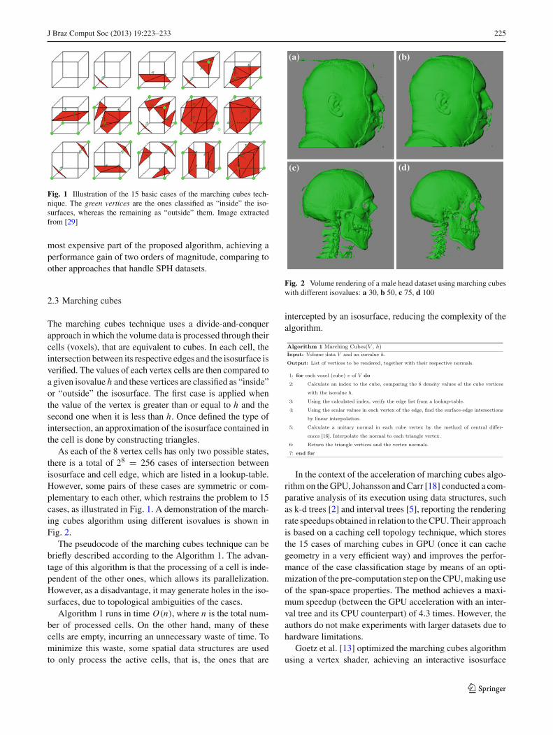
Fig. 1 Illustration of the 15 basic cases of the marching cubes tech-nique. The green vertices are the ones classified as “inside” the iso-surfaces, whereas the remaining as “outside” them. Image extractedfrom [29]

most expensive part of the proposed algorithm, achieving aperformance gain of two orders of magnitude, comparing toother approaches that handle SPH datasets.

2.3 Marching cubes

The marching cubes technique uses a divide-and-conquerapproach in which the volume data is processed through theircells (voxels), that are equivalent to cubes. In each cell, theintersection between its respective edges and the isosurface isverified. The values of each vertex cells are then compared toa given isovalue h and these vertices are classified as “inside”or “outside” the isosurface. The first case is applied whenthe value of the vertex is greater than or equal to h and thesecond one when it is less than h. Once defined the type ofintersection, an approximation of the isosurface contained inthe cell is done by constructing triangles.

As each of the 8 vertex cells has only two possible states,there is a total of 28 = 256 cases of intersection betweenisosurface and cell edge, which are listed in a lookup-table.However, some pairs of these cases are symmetric or com-plementary to each other, which restrains the problem to 15cases, as illustrated in Fig. 1. A demonstration of the march-ing cubes algorithm using different isovalues is shown inFig. 2.

The pseudocode of the marching cubes technique can bebriefly described according to the Algorithm 1. The advan-tage of this algorithm is that the processing of a cell is inde-pendent of the other ones, which allows its parallelization.However, as a disadvantage, it may generate holes in the iso-surfaces, due to topological ambiguities of the cases.

Algorithm 1 runs in time O(n), where n is the total num-ber of processed cells. On the other hand, many of thesecells are empty, incurring an unnecessary waste of time. Tominimize this waste, some spatial data structures are usedto only process the active cells, that is, the ones that are

Fig. 2 Volume rendering of a male head dataset using marching cubeswith different isovalues: a 30, b 50, c 75, d 100

intercepted by an isosurface, reducing the complexity of thealgorithm.

In the context of the acceleration of marching cubes algo-rithm on theGPU, Johansson andCarr [18] conducted a com-parative analysis of its execution using data structures, suchas k-d trees [2] and interval trees [5], reporting the renderingrate speedups obtained in relation to theCPU. Their approachis based on a caching cell topology technique, which storesthe 15 cases of marching cubes in GPU (once it can cachegeometry in a very efficient way) and improves the perfor-mance of the case classification stage by means of an opti-mization of the pre-computation step on theCPU,making useof the span-space properties. The method achieves a maxi-mum speedup (between the GPU acceleration with an inter-val tree and its CPU counterpart) of 4.3 times. However, theauthors do not make experiments with larger datasets due tohardware limitations.

Goetz et al. [13] optimized the marching cubes algorithmusing a vertex shader, achieving an interactive isosurface

123

226 J Braz Comput Soc (2013) 19:223–233

reconstruction, but their approach does not use any accel-erating data structures to improve the overall performanceof the algorithm, obtaining a maximum speedup of approxi-mately 2.0 times.

Newman andYi [32] developed an in-depth research aboutthe possibilities of developing the marching cubes tech-nique, describing their respective properties, extensions andattempts to solve its limitations. However, the paper onlyshows the differences between these possibilities in termsof algorithm complexity as well as visualization results, anddoes not make an analysis with volume datasets.

Smistad et al. [43] presented an implementation of themarching cubes algorithm written in OpenCL [37] that runsentirely in the GPU. Like [6], it uses the idea of histogrampyramids to generate the output stream of vertices to be ren-dered and runs as fast as CUDA and shader implementations,providing a very efficient storage scheme as well. However,the drawback of their implementation lies on the interoper-ability between OpenCL and OpenGL.

Concerning recent applications that make use of themarching cubes algorithm in GPU, Dembogurski et al. [7]used a marching cubes histogram pyramid implementationfor a procedural terrain generation; Donlon et al. [8] acceler-ated the visualization and quantification of MRI datasets tohelp in the treatment of patients that suffer from rheumatoidand psoriatic arthritis; Kim et al. [21] presented a methodfor computing the surfaces of a protein molecule in inter-active time; Lang et al. [23] developed an environment forfast and automated analysis of large SBFSEM (serial block-face scanning electronmicroscopy) datasets to extract neuronmorphologies.

2.4 Accelerating data structures

There are several classes of data structures that are very usefulto avoid the processing of empty cells. One of them consistsof interval-based representations, which uses cell intervals togroup cells [32]. The advantage of this type of representationis in its flexibility, being applied not only on regular grids,but also on non-regular grids, once it works from an intervalspace, instead of using the mesh space itself.

The main methods of this class are based on a represen-tation called span-space [28], where each cell of the volumedata is mapped to a two-dimensional point, whose coordi-nates x and y correspond, respectively, to the minimum andmaximum values among the eight vertices that constitute acell. From a given isovalue h, the points of the span-spacethat represent the active cells are the ones where x ≤ h andy ≥ h.

A general scheme of the span-space is shown in Fig. 3.The blue area corresponds to the active cells of a volume dataand the yellow areas to the cells that are not rendered, dueto the fact that x > h (yellow area located right of the blue

Fig. 3 Representation of the span-space proposed by Livnat et al. [28]

area) or y < h (yellow area located below the blue area). Nocell can be mapped to the red area, once x is never greaterthan y.

This section describes some spatial data structures andhow they can be used to improve the performance of themarching cubes algorithm.

2.4.1 k-d tree

The k-d tree [2] is a special case of the binary search tree,used to organize points located in a k-dimensional space.Each non-leaf node represents a splitting hyperplane thatdivides the space into two parts in a specific direction, whichis defined according to the depth of this node in the tree.The left subtree contains all the points located at the left ofthe hyperplane and the right subtree contains the ones to theright. The leaf nodes store one point each.

In the marching cubes algorithm, the volume data ismapped onto a span-space before constructing the tree, oncethe queries in the k-d tree are faster whenworkingwith pointsin a 2D plane rather than in a 3D space. Furthermore, everynode stores a point in the span-space, instead of storing thepoints only in the leaves. The construction takes O(n log n)time, where n is the total number of cells in the volume data,and demands a storage space of O(n).

When searching in the tree, given an isovalue h, it willtraverse only the nodes that correspond to the active cells ofthe volume data. Thus, the query takes O(

√n + p) time,

where p is the number of active cells.

2.4.2 Interval tree

The interval tree [5] is an ordered tree used to store intervalsof values in 1D. Similarly to the k-d tree, it is an extension

123

J Braz Comput Soc (2013) 19:223–233 227

of the binary search tree, and allows an efficient search of allintervals that overlap with a given interval or point.

The root of the tree stores a value that corresponds tothe median of the endpoints of all intervals and a list ofintervals that contain this value. The left subtree stores theintervals that are completely below the median and the rightsubtree stores the ones completely above the median. Then,the process is repeated recursively for each subtree. It takesa construction time of O(n log n) and, like the k-d tree, astorage space of O(n).

The span-space is suitable for constructing an interval tree.In this case, the intervals correspond to the volume cells, andthe endpoints are the minimum and maximum values of thecell, which stands for its coordinates in the span-space.

Searching in an interval tree takes O(log n + p) time,where p is the number of active cells, which makes it moreefficient than the k-d tree. On the other hand, it demandshigher memory space.

2.4.3 Quadtree and octree

A quadtree [12] is a tree data structure where every non-leaf node has exactly four children. It is used to partition aregion in a 2D space into four equal regions (or quadrants).These regions are then partitioned into other four subregions,and so on, until the subregion is empty, which characterizesa leaf node. The 3D analogous structure of a quadtree iscalled octree, which partitions a 3D space region into eightsubregions (or octants).

Once the span-space is a 2D space, it can be represented byaquadtree. Let l be the number of bits used to store the volumedata values, which means that there are 2l possible values(ranging between 0 and 2l − 1) for a vertex cell. Thus, thespan-space is a 2l ×2l region, and the points correspond to themapped cells. Every node in the tree stores the informationof a point in the span-space.

However, more than one cell can be mapped to a samepoint in the span-space. To overcome this problem, each nodein the quadtree also stores a pointer to a list of the volumedata cells that were mapped to this point. Then, the queriescan be made as usual, traversing the nodes corresponding tothe active cells.

In the octree case, the tree is built directly from the volumedata. However, in case of non-regular grids (i.e., when vol-ume dimension is not a power of two), the subregions havedifferent sizes, once we are partitioning cell regions.

3 Methodology

The significant evolution of the programmability of thegraphics hardware has allowed the isosurface extraction pro-cedure to be accelerated by the GPU, taking advantage of

its parallel architecture. However, the bus used to establisha communication between the CPU and the GPU is a bot-tleneck for this acceleration, which means that transferringall the tasks to the GPU may not be the best solution. Thus,in order to maximize the performance of this procedure, anadequate planning of the graphics pipeline is needed, pickingup the tasks that can be run on the CPU and the ones that canbe transferred to the GPU, as well as a proper use of all thememory hierarchy. Some proposals of graphics pipeline forisosurface extractionweremade byBuatois et al. [3], Johans-son [17], Martin et al. [31], Pascucci [38], Reck et al. [40],and Tatarchuk et al. [44].

The methodology proposed in this work is restricted tothe marching cubes technique, rather than generalizing tothe isosurface extraction process. Figure 4 shows a generalscheme, composed of six stages. At the Stage 1, the CPUreads a volume dataset of dimensions Nx × Ny × Nz , whichis then allocated both in themainmemory (RAM, used by theCPU) and in the video memory (VRAM, used by the GPU).Except for the octree, an extra memory space is allocated forthe span-space related to the volume data.

Later, one of the spatial data structures described inSect. 2.4 is constructed from the volume data and stored onlyin the main memory (stage 2). Then, the volume data is freedfrom the main memory, but it remains allocated in the videomemory.

Algorithm 2 details the two aforementioned stages of thescheme. Once the preprocessing stage is done, the march-ing cubes algorithm is started (stage 3). From an isovalue hspecified by the user, the CPU performs a search in the datastructure, traversing only the nodes that correspond to theactive volume cells, and creating a list of these cells, whichis then transferred to the GPU via communication bus.

With the list of active cells and the isovalue h, the march-ing cubes algorithm then proceeds on the GPU. Each cell isclassified into one of the 15 cases of marching cubes (shownin Fig. 1) by comparing h to the eight cell vertices. From thiscomparison, a cell index is created and then used to define thenumber of vertices needed to render the isosurface contained

123

228 J Braz Comput Soc (2013) 19:223–233

Fig. 4 Our method for acceleration of the marching cubes algorithm.Stages 1 and 2 are responsible for the preprocessing stage; stages 3 to5 correspond to the execution of marching cubes and stage 6 makes

the display of vertices on the screen. Green boxes stand for the actionsexecuted on CPU, whereas the orange boxes the ones on GPU

in the cell. After this procedure is done for all active cells,the total number of vertices to be output can be determined,which will define the exact size of video memory needed toallocate two vertex buffers: one for storing these vertices andother for their respective normals (stage 4).

After that, the list of active cells is traversed by the GPUonce more to generate the triangles that comprise the iso-surfaces (stage 5). For each active cell of the list, the GPUcalculates the isosurface intersections with the 12 edges ofthe cell by interpolating the vertices and the normals calcu-lated by the GPU from the volume data. Once the cell indexand the intersections are found, the GPU obtains the list ofvertices and normals related to the isosurface, writing themin the respective vertex buffers. Finally, the volume data isrendered from these buffers (stage 6).

All the procedures executed by the GPU are parallelized,once the results obtained from a cell are independent of theothers. However, the speedup achieved with the accelerationof the marching cubes relies on the way this parallelizationoccurs. When a task is assigned to the GPU, it creates aspecific amount of blocks.1 All of these blocks contain aspecific number of threads (which is the same for all blocks),responsible for running a part of this task.

The amount of blocks to be created depends on the numberof active cells and the number of threads per block, alsoknown as block size. The block size is chosen in such away that it is neither too low, assigning much work for allthreads and not maximizing the task performance at all, nortoo high, causing an overhead of starting and terminatingthreads.

The parallel processing of the list of active cells is madefrom a specific program, called GPU kernel. In our work, theGPU kernel was implemented using the CUDA architecture.

1 Concept from CUDA programming model [35].

In addition to the algorithms that are responsible for the exe-cution of the marching cubes technique, some of the GPUinherent resources were employed in order to improve therendering rate of the volume data. Among these resourcesare the use of texture memory, which is faster for handlingread-only data, to store the lookup-tables employed by themarching cubes algorithm and the volume data itself, and theuse of sharedmemory, which permits the data sharing amongthreads contained in a same block, besides being faster thanthe standard videomemory. In theGPUmarching cubes algo-rithm, the shared memory is used to compute, for each activecell, the intersections between an isosurface contained in thecell and the cell edges.

Thepseudocodes of the following algorithmswere adaptedfrom [36]. Before the execution of these algorithms, therespective number of blocks (as well as their sizes) usedto help on the parallelization of their procedures are deter-mined.

Algorithm 3 represents the first step of the execution ofmarching cubes in GPU (stage 4 of Fig. 4). The goal of thisalgorithm is to calculate the exact amount of video memorythat will be used to store the vertices and the normals relatedto the volume data. Once this amount is obtained, the GPUallocates the appropriate space in the vertex buffers, whichwill then store the vertices to be output and their respectivenormals.

Once this procedure is done, the Algorithm 4 is started.It is important to point out the repetition of the calculationof the cell indexes (line four of the Algorithms 3 and 4),which in GPU is faster than storing the results provided byAlgorithm 3 in an array and retrieving them in the subse-quent algorithm. Later, the vertex and normal buffers (calledP and N, respectively) are filled and the volume data isvisualized, thus finishing the steps of the marching cubestechnique.

123

J Braz Comput Soc (2013) 19:223–233 229

4 Experimental results

The tests were executed on an AMD Phenom II X6 1090T3.2 GHz processor with 8 GB of RAM, and an NVIDIAGeForce GTS 450 with 1 GB of VRAM (together with itsmost recent drivers), using a C-like programming language,OpenGL 4.2 and CUDA 4.1 APIs.

The experiments were made using 8-bit datasets from [1]and [45], where each scalar value ranges from 0 to 255. Table

Table 1 List of volume datasets with their respective sizes in voxels,isovalues, number of triangles and memory space allocated during exe-cution of marching cubes algorithm (in megabytes)

Volume name Dimensions Isovalue # Triangles Space (MB)

Fuel 64 × 64 × 64 10 11,534 0.51

Hydrogen atom 128 × 128 × 128 20 47,864 3.09

Angiography 256 × 320 × 128 80 84,974 11.94

Engine 256 × 256 × 128 155 207,592 12.75

Lobster 301 × 324 × 56 45 317,024 12.46

Head 128 × 256 × 256 50 544,588 20.46

Bonsai 256 × 256 × 256 45 858,118 35.64

Knee 379 × 229 × 205 60 1,027,838 40.49

Sheep heart 352 × 352 × 256 80 1,397,064 61.87

Aneurism 512 × 512 × 512 45 835,068 147.11

1 shows a list of volume datasets used in the tests, togetherwith their respective dimensions (in voxels), isovalues (inputto the marching cubes algorithm), number of triangles ren-dered in the screen (which depends on the isovalue), andmemory space allocated during the execution of the march-ing cubes algorithm, which corresponds to the size of thevolume datasets (1 byte per voxel) plus the amount of thevertex and normal buffers (4 bytes per vertex and normal,which leads to a total of 24 bytes per triangle, once thereare two buffers). The isovalues for “Fuel”, “Hydrogen atom”and “Engine” datasets were the same as those used by [18],so that a more accurate comparison can be made. The resultsof the rendering of each dataset, made from the applicationdescribed in this work, are shown in Fig. 5.

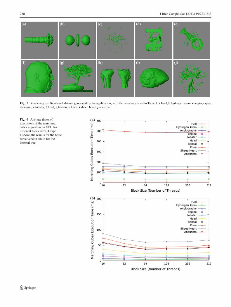
Figure 6 shows two plots that illustrate the average time (inmilliseconds) of 50 executions of the marching cubes imple-mentation on the GPU for different block size values, usingeach of the volume datasets and their respective isovalueslisted in Table 1. The plot (a) stands for the executions of abrute force implementation of the marching cubes algorithmthat runs without the aid of accelerating data structures andsequentially traverses all voxels of a volume dataset (includ-ing the empty ones), and (b) the executions using an intervaltree to store the voxels from the datasets. From both plots, itcan be noticed that for block sizes of 64 and higher, the run-ning time of the marching cubes increases very slightly, andit does not rely on whether a data structure is used or not foracceleration. In other words, for any data structure used inthe marching cubes algorithm, the behavior of the curves inthe plot will be the same. As mentioned in Sect. 3, althougha higher number of threads means higher parallelization, thetime spent to create the threads also gets higher, hence sta-bilizing the performance. Thus, all the tests were run with ablock size value of 64.

Table 2 shows the average frame rate of the execution ofmarching cubes algorithm inCPUandGPU, for all data struc-tures described in Sect. 2.4, and comparing to their respectiveCPU versions of the algorithm. These results do not considerthe time spent on the pre-processing stages (volume datareading and data structure construction), regarding only theevents that occur between the search in the data structure andthe volume display on the screen (Stages 3–6 of Fig. 4).

As it is possible to observe, the interval tree provided thebest results (highlighted in bold in Table 2), not only amongall the data structures used in the tests, but also in the accel-eration factor compared to the CPUmarching cubes, achiev-ing a maximum speedup of 18.2 times for the “Aneurism”dataset. This result was expected because the interval treehas asymptotically a better query time than the other struc-tures. Furthermore, the obtained speedups are superior thanthose of Johansson and Carr’s approach [18], which achievesa maximum speedup of 4.3 times (for the “Hydrogen Atom”dataset and the interval tree) using pre-calculated normals,

123

230 J Braz Comput Soc (2013) 19:223–233

Fig. 5 Rendering results of each dataset generated by the application, with the isovalues listed in Table 1. a Fuel, b hydrogen atom, c angiography,d engine, e lobster, f head, g bonsai, h knee, i sheep heart, j aneurism

Fig. 6 Average times ofexecutions of the marchingcubes algorithm on GPU fordifferent block sizes. Grapha shows the results for the bruteforce version and b for theinterval tree

123

J Braz Comput Soc (2013) 19:223–233 231

Table 2 Average frame rate (inframes per second) of theexecution of marching cubesalgorithm in CPU and GPU,with different data structures,comparing against the bruteforce version

Values between parenthesiscorrespond to the accelerationfactor related to their respectivedata structure versions ofmarching cubes in CPU for eachvolume dataset

Volume name Brute force k-d tree Interval tree Quadtree Octree

CPUFuel 83.3 105.6 114.4 108.0 98.3

Hydrogen atom 17.5 23.4 25.6 24.0 19.2

Angiography 7.5 12.9 14.1 13.6 10.7

Engine 4.6 5.2 5.7 5.5 4.8

Lobster 3.2 3.7 4.1 3.9 3.6

Head 1.8 2.0 2.3 2.1 1.9

Bonsai 1.2 1.3 1.6 1.4 1.3

Knee 1.1 1.2 1.4 1.3 1.1

Sheep heart 0.8 0.9 1.0 0.9 0.8

Aneurism 0.6 0.9 1.3 1.2 0.7

GPUFuel 195.4 (2.3) 220.7 (2.1) 246.4 (2.2) 229.9 (2.1) 205.7 (2.1)

Hydrogen Atom 77.0 (4.4) 142.8 (6.1) 165.0 (6.4) 149.5 (6.2) 96.5 (5.0)

Angiography 24.7 (3.3) 109.6 (8.5) 133.7 (9.5) 89.2 (6.6) 58.7 (5.5)

Engine 26.6 (5.8) 61.0 (11.7) 81.1 (14.2) 56.8 (10.3) 38.4 (8.0)

Lobster 30.1 (9.4) 42.8 (11.6) 58.5 (14.3) 29.8 (7.6) 27.4 (7.6)

Head 17.9 (9.9) 22.7 (11.4) 35.8 (15.6) 28.9 (13.8) 20.9 (11.0)

Bonsai 10.7 (8.9) 13.2 (10.2) 25.9 (16.2) 18.7 (13.4) 11.5 (8.8)

Knee 8.2 (7.4) 9.7 (8.1) 22.4 (16.0) 10.7 (8.2) 9.1 (8.2)

Sheep Heart 6.3 (7.9) 7.4 (8.2) 16.3 (16.3) 8.9 (9.9) 6.6 (8.3)

Aneurism 2.1 (3.5) 10.2 (11.3) 23.7 (18.2) 11.9 (9.9) 9.5 (13.5)

while the method proposed in this paper calculates them on-the-fly.

Another important fact to be pointed out is the perfor-mance of quadtree, which obtained a better frame rate thanthe k-d tree and the octree, standing only behind the intervaltree. It achieved a maximum speedup of 13.8 times for the“Head” dataset. For the other datasets, excluding the “Fuel”,the speedup was between 6.2 and 10.3.

Concerning the building time of the data structures,quadtree had amuch higher performance than the other ones,as shown in Fig. 7. For all datasets used in the tests, the build-ing time of the quadtree was verymuch smaller than the otherdata structures, not having a significant gain of time as thevolume datasets get larger, which is very efficient for realapplications that process great amounts of volume data. Forthe rest of the data structures, the building time increasesconsiderably among the datasets.

Octree provided the second best building times. Eventhough its building algorithm is similar to the one of quadtree,the fact that it is applied in the 3D space brings on a higherwaste of time, once the total number of subdivisions is higher.In third place, comes the k-d tree, which has a worse build-ing time than the octree because of the successive executionsof the algorithm that finds the median of the points locatedin the span-space. Finally, interval tree achieved the worst

building times among the tested data structures. It happeneddue to the time spent in sorting the cell lists, which has ahigher time complexity than finding a median.

The bottleneck of this approach resides on the fact thatthe searches in the data structures are done on the CPU. Itis feasible to implement all of the data structure algorithmson the GPU, as well as storing the data structure itself in thevideo memory, but since most of the tree search algorithmsare recursive and CUDA does not support recursions, if non-recursive versions of these algorithms were implemented onthe GPU, there would have a large waste of time and space tocreate stacks and loopsused to simulate the eventual recursivecalls.

5 Conclusions and future work

Volume visualization techniques allow users to explore andanalyze tridimensional data, which benefit several knowl-edge domains, such as biology, medicine, meteorology,oceanography, geology. A challenging task of volume visu-alization is the development of efficient algorithms for rep-resenting, manipulating and rendering complex and largedatasets.

123

232 J Braz Comput Soc (2013) 19:223–233

Fig. 7 Average building timesof the data structures for eachvolume dataset

This paper described a comparative analysis among fourdifferent spatial data structures for speeding up the marchingcubes algorithm through graphics processing units, togetherwith an approach using CUDA framework. Time complexityof the algorithmdepends on the volumedata cells that containan isosurface, instead of the total number of cells, avoidingthe processing of empty cells.

Experimental results obtained from several volumetricdatasets demonstrate that it was possible to accelerate themarching cubes algorithm by a factor of approximately 18times when compared to the CPU approach.

Among the four data structures described in this paper,interval tree provided the best rendering rates, but the timespent in building the structure was relatively high. On theother hand, quadtree achieved very satisfactory buildingtimes, even for large volume datasets, besides slightly lowerrendering rates compared to those of the acceleration withan interval tree. However, since the building of a data struc-ture is done only once, while the search is performed when-ever the volume needs to be rendered, it is more worth-while to use the interval tree rather than the quadtree in thiscase.

Directions for future work include the implementationof the data structures mentioned in this paper on the GPU,together with their respective building and searching oper-ations so that they can be done in parallel, and an exten-sion of the proposed method to open frameworks, such asOpenCL [37], once that CUDA framework is restricted toNVIDIA [35] graphic cards. Furthermore, a case study withmore powerful graphic cards (such as those from NVIDIAKepler architecture) is desired as well.

Acknowledgments The authors are grateful to FAPESP, CNPq, andNational Institute of Science and Technology in Medicine Assisted byScientific Computing (INCT/MACC) for the financial support.

References

1. The volume library. http://lgdv.cs.fau.de/External/vollib2. Bentley J (1975) Multidimensional binary search trees used for

associative searching. Commun ACM 18(9):509–5173. Buatois L, Caumon G, Lévy B (2006) GPU accelerated isosurface

extraction on tetrahedral grids. In: Advances in visual comput-ing. Lecture notes in computer science, vol 4291, Springer, Berlin,pp 383–392

4. Chan S, Purisima E (1998) A new tetrahedral tesselation schemefor isosurface generation. Comput Graph 22(1):83–90

5. Cignoni P, Marino P, Montani C, Scopigno R (1997) Speedingup isosurface extraction using interval trees. IEEE Trans VisualComput Graph 3:158–170

6. CiznickiM,KierzynkaM,KurowskiK,LudwiczakB,NapieralaK,Palczynski J (2011) Efficient isosurface extraction using marchingtetrahedra and histogram pyramids onmultiple GPUs. In: Proceed-ings of the 9th international conference on parallel processing andapplied mathematics, Torun, Poland, pp 343–352

7. Dembogurski B, Clua E,VieiraM, Leta F (2008) Procedural terraingeneration at GPU level with marching cubes. In: Proceedings ofthe VII Brazilian symposium of games and digital entertainment—computing track, Belo Horizonte, MG, Brazil, pp 37–40

8. Donlon B, Veale D, Brennan P, Gibney R, Carr H, Rainford L,Ng C, Pontifex E, McNulty J, FitzGerald O, Ryan J (2012) MRI-based visualisation and quantification of rheumatoid and psoriaticarthritis of the knee. In: Visualization in medicine and life sciencesII, mathematics and visualization, Springer, pp 45–59

9. Dürst M (1988) Letters: additional reference to marching cubes.ACM Comput Graph 22(4):72–73

10. Dyken C, Ziegler G, Theobalt C, Seidel H (2008) High-speedmarching cubes using histopyramids. Comput Graph 27(8):2028–2039

11. Elvins T (1992) A survey of algorithms for volume visualization.SIGGRAPH Comput Graph 26(3):194–201

12. Finkel R, Bentley J (1974) Quad trees: a data structure for retrievalon composite keys. Acta Inf 4(1):1–9

13. Goetz F, Junklewitz T, Domik G (2005) Real-time marching cubeson the vertex shader. In: Eurographics. Dublin, Ireland

14. Gong F, Zhao X (2010) Three-dimensional reconstruction of med-ical image based on improved marching cubes algorithm. In: Pro-ceedings of the international conference on machine vision andhuman-machine interface, Kaifeng, China, pp 608–611

123

J Braz Comput Soc (2013) 19:223–233 233

15. Guéziec A, Hummel R (1995) Exploiting triangulated surfaceextraction using tetrahedral decomposition. IEEE Trans VisualComput Graph 1(4):328–342

16. JeffreysH, JeffreysB (1988)Central differences formula. In:Meth-ods of mathematical physics, Cambridge University Press, Cam-bridge, pp 284–286

17. Johansson G (2005) Accelerating isosurface extraction by cachingcell topology with graphics hardware. Master’s thesis, UniversityCollege Dublin, Ireland

18. Johansson G, Carr H (2006) Accelerating marching cubes withgraphics hardware. In: Proceedings of the conference of the cen-ter for advanced studies on collaborative research. Toronto, ON,Canada

19. Kaufman A (1991) Volume visualization. IEEE Computer SocietyPress, Los Alamitos

20. Keppel E (1975) Approximating complex surfaces by triangulationof contour lines. IBM J Res Dev 19(1):2–11

21. Kim B, KimK, Seong J (2012) GPU accelerated molecular surfacecomputing. Appl Math Inf Sci 6(1S):185S–194S

22. Lacroute P (1996) Fast volume rendering using a shear-warp fac-torization of the viewing transformation. PhD thesis, Stanford Uni-versity, Stanford, CA, USA

23. Lang S, Drouvelis P, Tafaj E, Bastian P, Sakmann B (2011)Fast extraction of neuron morphologies from large-scale SBFSEMimage stacks. J Comput Neurosci 31(3):533–545

24. Lengyel E (2010) Transition cells for dynamic multiresolutionmarching cubes. J Graph GPU Game Tools 15(2):99–122

25. Levoy M (1990) Efficient ray tracing of volume data. ACM TransGraph 9(3):245–261

26. Li T, Xie M, Zhao W, Wei Y (2010) Shear-warp rendering algo-rithm based on radial basis functions interpolation. In: Proceedingsof the 2nd international conference on computermodeling and sim-ulation, Sanya, China, pp 425–429

27. Liu B, Clapworthy G, Dong F (2009) Accelerating volume raycast-ing using proxy spheres. Comput Graph Forum 28(3):839–846

28. Livnat Y, Shen HW, Johnson R (1996) A near optimal isosurfaceextraction algorithm using the span space. IEEETransVisual Com-put Graph 2(1):73–84

29. LorensenW, Cline H (1987) Marching cubes: a high resolution 3Dsurface construction algorithm. Comput Graph 21(4):163–169

30. Lum EB, Wilson B, liu Ma K (2004) High-quality lighting andefficient pre-integration for volume rendering. In: Proceedings ofthe joint Eurographics—IEEETVCG symposium on visualization,pp 25–34

31. Martin S, Shen HW, McCormick P (2010) Load-balanced isosur-facing on multi-GPU clusters. In: Proceedings of the Eurograph-ics symposium on parallel graphics and visualization, Norrküping,Sweden, pp 91–100

32. Newman T, Yi H (2006) A survey of themarching cubes algorithm.Comput Graph 30(5):854–879

33. Nielson GM, Hamann B (1991) The asymptotic decider: resolv-ing the ambiguity in marching cubes. In: Proceedings of the 2ndconference on visualization, San Diego, CA, USA, pp 83–91

34. Nurzynska K (2009) 3D object reconstruction from parallel cross-sections. In: Bolc L, Kulikowski J, Wojciechowski K (eds) Com-puter vision and graphics. Lecture notes in computer science, vol5337, Springer, Berlin, pp 111–122

35. NVIDIA CUDA C programming guide version 3.2. http://developer.download.nvidia.com/compute/cuda/3_2_prod/toolkit/docs/CUDA_C_Programming_Guide.pdf

36. NVIDIA (2012) CUDA C/C++ SDK code examples. http://developer.nvidia.com/cuda-cc-sdk-code-samples

37. OpenCL The khronos group. http://www.khronos.org/opencl/38. Pascucci V (2004) Isosurface computation made simple: hardware

acceleration, adaptive refinement and tetrahedral stripping. In: Pro-ceedings of the joint Eurographics—IEEE TVCG symposium onvisualization, Konstanz, Germany, pp 293–300

39. Pöthkow K, Weber B, Hege HC (2011) Probabilistic marchingcubes. Comput Graph Forum 30(3):931–940

40. Reck F, Dachsbacher C, Grosso R, Greiner G, Stamminger M(2004) Realtime isosurface extraction with graphics hardware. In:Proceedings of theEurographics 2004 short presentations and inter-active demos, Grenoble, France, pp 33–36

41. Schindler B, Fuchs R, Waser J, Peikert R (2011) Marchingcorrectors—fast and precise polygonal isosurfaces of SPH data.In: Proceedings of the 6th international smoothed particle hydrody-namics European research interest community (SPHERIC) work-shop, Hamburg, Germany, pp 125–132

42. Schlegel P, Pajarola R (2009) Layered volume splatting. In:Advances in visual computing, lecture notes in computer science,vol 5876, Springer, pp 1–12

43. Smistad E, Elster AC, Lindseth F (2011) Fast surface extractionand visualization of medical images using openCL and GPUs. In:Proceedings of the joint workshop on high performance and dis-tributed computing for medical imaging, Toronto, Canada

44. Tatarchuk N, Shopf J, DeCoro C (2007) Real-time isosurfaceextraction using the GPU programmable geometry pipeline. In:Proceedings of the ACM SIGGRAPH 2007 courses, San Diego,CA, USA, pp 122–137

45. Volvis: volume datasets. http://www.volvis.org46. Wang Z, Fan B, Li N, Zhang H (2009) Iso-surface extraction and

optimization method based on marching cubes. In: Proceedingsof the international conference on semantics, knowledge and grid,Zhuhai, China, pp 458–460

47. Westover L (1990) Footprint evaluation for volume rendering. In:Proceedings of the 17th annual conference on computer graphicsand interactive techniques, Dallas, TX, USA, pp 367–376

48. Wilhelms J (1990) A coherent projection approach for direct vol-ume rendering. Technical report of University of California, SantaCruz, CA, USA

49. Zhu S, Gu YL (2008) Volume rendering algorithm of irregularvolume based on cell projection. Comput Eng Appl 44(15):68–70

50. Ziegler G, Tevs A, Theobalt C, Seidel HP (2006) On-the-fly pointclouds through histogram pyramids. In: Proceedings of the 11thinternational fall workshop on vision, modeling and visualization,Aachen, Germany, pp 137–144

123